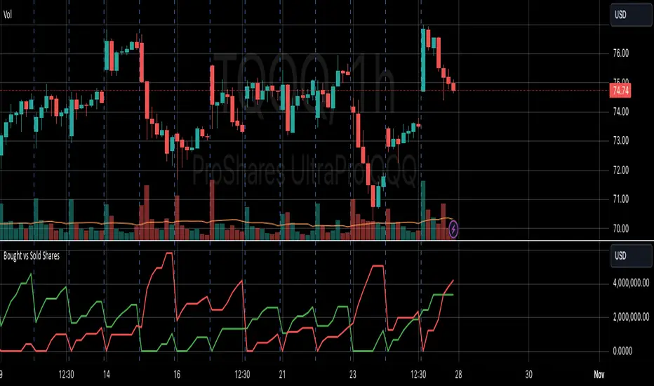
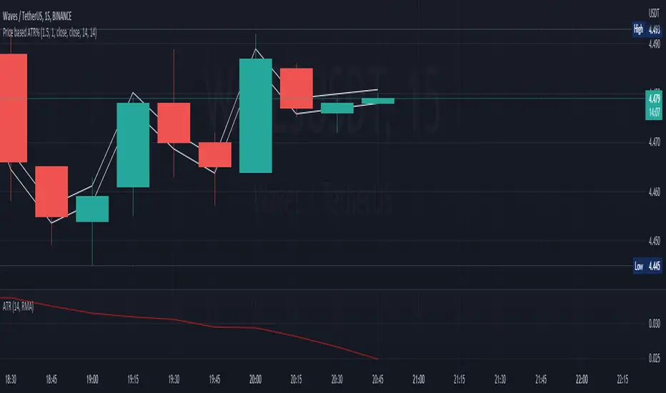
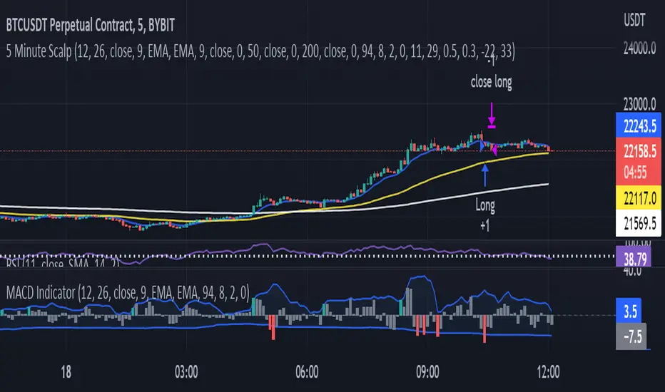
Capiba Directional Momentum Oscillator (ADX-based)
🇬🇧 English
Summary
The Capiba ADX is a momentum oscillator that transforms the classic ADX (Average Directional Index) into a much more intuitive visual tool. Instead of analyzing three separate lines (ADX, DI+, DI-), this indicator consolidates the strength and direction of the trend into a single histogram that oscillates around the zero line.
The result is a clear and immediate reading of market sentiment, allowing traders to quickly identify who is in control—buyers or sellers—and with what intensity.
How to Interpret and Use the Indicator
The operation of the Capiba ADX is straightforward:
Green Histogram (Above Zero): Indicates that buying pressure (DI+) is in control. The height of the bar represents the magnitude of the bullish momentum. Taller green bars suggest a stronger uptrend.
Red Histogram (Below Zero): Indicates that selling pressure (DI-) is in control. The "depth" of the bar represents the magnitude of the bearish momentum. Lower (more negative) red bars suggest a stronger downtrend.
Zero Line (White): This is the equilibrium point. Crossovers through the zero line signal a potential shift in trend control.
Crossover Above: Buyers are taking control.
Crossover Below: Sellers are taking control.
Reference Levels (Momentum Strength)
The indicator plots three fixed reference levels to help gauge the intensity of the move:
0 Line: Equilibrium.
100 Line: Signals significant directional momentum. When the histogram surpasses this level, the trend (whether bullish or bearish) is gaining considerable strength.
200 Line: Signals very strong directional momentum, or even potential exhaustion conditions. Moves that reach this level are powerful but may also precede a consolidation or reversal.
Usage Strategy
Trend Confirmation: Use the indicator to confirm the direction of your analysis. If you are looking for long positions, the Capiba ADX should ideally be green and, preferably, rising.
Strength Identification: Watch for the histogram to cross the 100 and 200 levels to validate the strength of a breakout or an established trend.
Entry/Exit Signals: A zero-line crossover can be used as a primary entry or exit signal, especially when confirmed by other technical analysis tools.
Acknowledgements
This indicator is the result of adapting knowledge and open-source codes shared by the vibrant TradingView community.
Komut dosyalarını "entry" için ara
Capiba Ultimate Suite (RSI, MA Cloud & Volatility)
🇬🇧 English
Summary
This indicator, Capiba Ultimate Suite, is a powerful compilation of various open-source technical analysis tools, refined and integrated into a single, cohesive, and functional package. The goal is to provide a complete system with clear entry and exit signals, ideal for traders operating in trending and volatile markets.
The combination of a custom momentum oscillator (Ultimate RSI), a moving average cloud for trend definition, and a volatility oscillator for range analysis transforms this script into a true trading suite.
Disclaimer: This indicator is most effective in markets with a defined trend (bullish or bearish) and may generate less reliable signals during periods of strong consolidation.
Components and How to Use
Ultimate RSI with Crossover Signals (Entries and Exits)
What it is: A variation of the classic RSI, designed to be more reactive to price movements.
Entry Signals (Buy): A green arrow (▲) appears below the candle when the Ultimate RSI line crosses above its momentum line (EMA). This is a signal of a potential start of an upward move.
Exit Signals (Sell): A red arrow (▼) appears above the candle when the Ultimate RSI crosses below its momentum line. This is a signal of potential weakening or trend reversal.
Moving Average Cloud (Trend Filter)
What it is: A cloud formed by the space between a short-term moving average (default 55) and a long-term one (default 233).
How to use for signal validation:
Uptrend: When the cloud is green (Short MA > Long MA), buy signals (▲) are strengthened. Sell signals can be seen as partial profit-taking.
Downtrend: When the cloud is red (Short MA < Long MA), sell signals (▼) are strengthened. Buy signals should be treated with extreme caution as they are against the main trend.
Candle Coloring (Quick Momentum Reading)
Lime Green: Strong bullish momentum (RSI > 50 and above its EMA).
Red: Strong bearish momentum (RSI < 50 and below its EMA).
Blue: Overbought level reached.
Yellow: Oversold level reached.
Volatility Ruler (Breakout Analysis)
What it is: The green (high) and red (low) lines mark the range of the last 'N' candles. The Vol: X.XX label on the right measures the current volatility against its historical average.
How to use:
Vol < 1.00: Contracting volatility ("Squeeze"). The market is "coiling the spring." Watch for an impending breakout of the range lines.
Vol > 1.00: Expanding volatility. Confirms the strength of a breakout that has already occurred. Very high values may indicate exhaustion.
Use the ruler to identify false breakouts: a candle closing outside the line but with a very low Vol value is more likely to be a false signal.
Acknowledgements
This indicator is the result of compiling and adapting open-source concepts and codes available in the TradingView community. Thanks to all the developers who share their knowledge.
>>>>>>>>>>>>>>>>>>>>>>>>>>>>>>>>>>>>>>>>>>>>>>>>>>>>>>>>>>>>>>>>>>>>>>>>
HA • EMA9/21 • Daily VWAP – Fixed Signals (v6)HA • EMA9/21 • Daily VWAP – Fixed Signals (v6)
Heikin Ashi EMA 9/21 + Daily VWAP Setup Indicator
Description
This indicator combines three proven concepts into one clean and practical trading tool:
Heikin Ashi Candles → smooth out price action and highlight trends more clearly.
EMA 9/21 → a classic momentum and trend filter.
Daily VWAP (Volume Weighted Average Price) → widely used by professionals as dynamic support and resistance.
How it works
Long Signal:
Triggered when Heikin Ashi turns bullish, EMA 9 is above EMA 21, and price crosses above the Daily VWAP.
Short Signal:
Triggered when Heikin Ashi turns bearish, EMA 9 is below EMA 21, and price crosses below the Daily VWAP.
For every signal the indicator automatically draws Entry, Stop-Loss, and Take-Profit levels directly on the chart:
Entry = price at the signal bar
Stop-Loss (SL) = recent swing low/high or ATR-based (configurable)
Take-Profit (TP) = calculated using the chosen Risk/Reward ratio
Features
✅ Instant signals (no repainting)
✅ Fixed horizontal lines for Entry, SL, and TP extending to the right side of the chart
✅ Customizable Risk/Reward ratio (default: 1.5)
✅ Choice between Swing-based or ATR-based stop-loss
✅ Alerts for both Long and Short signals
✅ Clean chart visualization without clutter
Use case
This tool is designed for traders who want clear, rule-based setups.
It provides easy-to-spot signals that can be used for manual trading, journaling, and backtesting.
⚠️ Note: This is not an automated trading strategy. Always confirm signals with your own analysis and apply proper risk management.
Trader Marks Trailing SL + TP (Long & Short, mirrored)📌 Trader Marks Trailing SL + TP (Long & Short, mirrored)
This script implements an advanced trailing stop and take-profit system for both long and short trades.
It combines fixed entry/TP levels with a progressive looping mechanism that dynamically adjusts the trailing stop.
🔑 Key Features
Long & Short mirrored
The script works symmetrically for both long and short setups.
Fixed or percentage-based Take-Profit
You can either set a fixed TP price or have it calculated automatically as entry ± percentage distance.
Progressive Trailing Stop with Looping Mechanism
The stop-loss moves progressively towards the take-profit depending on price development.
For longs, the SL only moves upward (never lower).
For shorts, the SL only moves downward (never higher).
The looping exponent (tightPower) controls how strongly the gap between price and SL “tightens” over time:
Smaller values (e.g. 1.0) → gentle tightening, SL follows loosely.
Larger values (e.g. 3.0) → aggressive tightening, SL closes in on price faster.
Dynamic Minimum Distance
Default: 0.9 % distance from price.
As soon as the stop-loss touches the current or previous candle → automatic switch to 1.5 %.
Once the next candle no longer touches the SL → it reverts back to 0.9 %.
Lock at TP
Option to pull the SL exactly to the TP level once it is reached.
Automatic Reset
If any inputs change (Entry, TP, Trade Direction), the SL can be re-initialized automatically.
🎨 Visualization
Blue line → Entry level
Teal line → Take-profit level
Red line → Dynamic trailing stop
The data window also shows whether the tight mode (1.5 %) is currently active.
Markov Chain [3D] | FractalystWhat exactly is a Markov Chain?
This indicator uses a Markov Chain model to analyze, quantify, and visualize the transitions between market regimes (Bull, Bear, Neutral) on your chart. It dynamically detects these regimes in real-time, calculates transition probabilities, and displays them as animated 3D spheres and arrows, giving traders intuitive insight into current and future market conditions.
How does a Markov Chain work, and how should I read this spheres-and-arrows diagram?
Think of three weather modes: Sunny, Rainy, Cloudy.
Each sphere is one mode. The loop on a sphere means “stay the same next step” (e.g., Sunny again tomorrow).
The arrows leaving a sphere show where things usually go next if they change (e.g., Sunny moving to Cloudy).
Some paths matter more than others. A more prominent loop means the current mode tends to persist. A more prominent outgoing arrow means a change to that destination is the usual next step.
Direction isn’t symmetric: moving Sunny→Cloudy can behave differently than Cloudy→Sunny.
Now relabel the spheres to markets: Bull, Bear, Neutral.
Spheres: market regimes (uptrend, downtrend, range).
Self‑loop: tendency for the current regime to continue on the next bar.
Arrows: the most common next regime if a switch happens.
How to read: Start at the sphere that matches current bar state. If the loop stands out, expect continuation. If one outgoing path stands out, that switch is the typical next step. Opposite directions can differ (Bear→Neutral doesn’t have to match Neutral→Bear).
What states and transitions are shown?
The three market states visualized are:
Bullish (Bull): Upward or strong-market regime.
Bearish (Bear): Downward or weak-market regime.
Neutral: Sideways or range-bound regime.
Bidirectional animated arrows and probability labels show how likely the market is to move from one regime to another (e.g., Bull → Bear or Neutral → Bull).
How does the regime detection system work?
You can use either built-in price returns (based on adaptive Z-score normalization) or supply three custom indicators (such as volume, oscillators, etc.).
Values are statistically normalized (Z-scored) over a configurable lookback period.
The normalized outputs are classified into Bull, Bear, or Neutral zones.
If using three indicators, their regime signals are averaged and smoothed for robustness.
How are transition probabilities calculated?
On every confirmed bar, the algorithm tracks the sequence of detected market states, then builds a rolling window of transitions.
The code maintains a transition count matrix for all regime pairs (e.g., Bull → Bear).
Transition probabilities are extracted for each possible state change using Laplace smoothing for numerical stability, and frequently updated in real-time.
What is unique about the visualization?
3D animated spheres represent each regime and change visually when active.
Animated, bidirectional arrows reveal transition probabilities and allow you to see both dominant and less likely regime flows.
Particles (moving dots) animate along the arrows, enhancing the perception of regime flow direction and speed.
All elements dynamically update with each new price bar, providing a live market map in an intuitive, engaging format.
Can I use custom indicators for regime classification?
Yes! Enable the "Custom Indicators" switch and select any three chart series as inputs. These will be normalized and combined (each with equal weight), broadening the regime classification beyond just price-based movement.
What does the “Lookback Period” control?
Lookback Period (default: 100) sets how much historical data builds the probability matrix. Shorter periods adapt faster to regime changes but may be noisier. Longer periods are more stable but slower to adapt.
How is this different from a Hidden Markov Model (HMM)?
It sets the window for both regime detection and probability calculations. Lower values make the system more reactive, but potentially noisier. Higher values smooth estimates and make the system more robust.
How is this Markov Chain different from a Hidden Markov Model (HMM)?
Markov Chain (as here): All market regimes (Bull, Bear, Neutral) are directly observable on the chart. The transition matrix is built from actual detected regimes, keeping the model simple and interpretable.
Hidden Markov Model: The actual regimes are unobservable ("hidden") and must be inferred from market output or indicator "emissions" using statistical learning algorithms. HMMs are more complex, can capture more subtle structure, but are harder to visualize and require additional machine learning steps for training.
A standard Markov Chain models transitions between observable states using a simple transition matrix, while a Hidden Markov Model assumes the true states are hidden (latent) and must be inferred from observable “emissions” like price or volume data. In practical terms, a Markov Chain is transparent and easier to implement and interpret; an HMM is more expressive but requires statistical inference to estimate hidden states from data.
Markov Chain: states are observable; you directly count or estimate transition probabilities between visible states. This makes it simpler, faster, and easier to validate and tune.
HMM: states are hidden; you only observe emissions generated by those latent states. Learning involves machine learning/statistical algorithms (commonly Baum–Welch/EM for training and Viterbi for decoding) to infer both the transition dynamics and the most likely hidden state sequence from data.
How does the indicator avoid “repainting” or look-ahead bias?
All regime changes and matrix updates happen only on confirmed (closed) bars, so no future data is leaked, ensuring reliable real-time operation.
Are there practical tuning tips?
Tune the Lookback Period for your asset/timeframe: shorter for fast markets, longer for stability.
Use custom indicators if your asset has unique regime drivers.
Watch for rapid changes in transition probabilities as early warning of a possible regime shift.
Who is this indicator for?
Quants and quantitative researchers exploring probabilistic market modeling, especially those interested in regime-switching dynamics and Markov models.
Programmers and system developers who need a probabilistic regime filter for systematic and algorithmic backtesting:
The Markov Chain indicator is ideally suited for programmatic integration via its bias output (1 = Bull, 0 = Neutral, -1 = Bear).
Although the visualization is engaging, the core output is designed for automated, rules-based workflows—not for discretionary/manual trading decisions.
Developers can connect the indicator’s output directly to their Pine Script logic (using input.source()), allowing rapid and robust backtesting of regime-based strategies.
It acts as a plug-and-play regime filter: simply plug the bias output into your entry/exit logic, and you have a scientifically robust, probabilistically-derived signal for filtering, timing, position sizing, or risk regimes.
The MC's output is intentionally "trinary" (1/0/-1), focusing on clear regime states for unambiguous decision-making in code. If you require nuanced, multi-probability or soft-label state vectors, consider expanding the indicator or stacking it with a probability-weighted logic layer in your scripting.
Because it avoids subjectivity, this approach is optimal for systematic quants, algo developers building backtested, repeatable strategies based on probabilistic regime analysis.
What's the mathematical foundation behind this?
The mathematical foundation behind this Markov Chain indicator—and probabilistic regime detection in finance—draws from two principal models: the (standard) Markov Chain and the Hidden Markov Model (HMM).
How to use this indicator programmatically?
The Markov Chain indicator automatically exports a bias value (+1 for Bullish, -1 for Bearish, 0 for Neutral) as a plot visible in the Data Window. This allows you to integrate its regime signal into your own scripts and strategies for backtesting, automation, or live trading.
Step-by-Step Integration with Pine Script (input.source)
Add the Markov Chain indicator to your chart.
This must be done first, since your custom script will "pull" the bias signal from the indicator's plot.
In your strategy, create an input using input.source()
Example:
//@version=5
strategy("MC Bias Strategy Example")
mcBias = input.source(close, "MC Bias Source")
After saving, go to your script’s settings. For the “MC Bias Source” input, select the plot/output of the Markov Chain indicator (typically its bias plot).
Use the bias in your trading logic
Example (long only on Bull, flat otherwise):
if mcBias == 1
strategy.entry("Long", strategy.long)
else
strategy.close("Long")
For more advanced workflows, combine mcBias with additional filters or trailing stops.
How does this work behind-the-scenes?
TradingView’s input.source() lets you use any plot from another indicator as a real-time, “live” data feed in your own script (source).
The selected bias signal is available to your Pine code as a variable, enabling logical decisions based on regime (trend-following, mean-reversion, etc.).
This enables powerful strategy modularity : decouple regime detection from entry/exit logic, allowing fast experimentation without rewriting core signal code.
Integrating 45+ Indicators with Your Markov Chain — How & Why
The Enhanced Custom Indicators Export script exports a massive suite of over 45 technical indicators—ranging from classic momentum (RSI, MACD, Stochastic, etc.) to trend, volume, volatility, and oscillator tools—all pre-calculated, centered/scaled, and available as plots.
// Enhanced Custom Indicators Export - 45 Technical Indicators
// Comprehensive technical analysis suite for advanced market regime detection
//@version=6
indicator('Enhanced Custom Indicators Export | Fractalyst', shorttitle='Enhanced CI Export', overlay=false, scale=scale.right, max_labels_count=500, max_lines_count=500)
// |----- Input Parameters -----| //
momentum_group = "Momentum Indicators"
trend_group = "Trend Indicators"
volume_group = "Volume Indicators"
volatility_group = "Volatility Indicators"
oscillator_group = "Oscillator Indicators"
display_group = "Display Settings"
// Common lengths
length_14 = input.int(14, "Standard Length (14)", minval=1, maxval=100, group=momentum_group)
length_20 = input.int(20, "Medium Length (20)", minval=1, maxval=200, group=trend_group)
length_50 = input.int(50, "Long Length (50)", minval=1, maxval=200, group=trend_group)
// Display options
show_table = input.bool(true, "Show Values Table", group=display_group)
table_size = input.string("Small", "Table Size", options= , group=display_group)
// |----- MOMENTUM INDICATORS (15 indicators) -----| //
// 1. RSI (Relative Strength Index)
rsi_14 = ta.rsi(close, length_14)
rsi_centered = rsi_14 - 50
// 2. Stochastic Oscillator
stoch_k = ta.stoch(close, high, low, length_14)
stoch_d = ta.sma(stoch_k, 3)
stoch_centered = stoch_k - 50
// 3. Williams %R
williams_r = ta.stoch(close, high, low, length_14) - 100
// 4. MACD (Moving Average Convergence Divergence)
= ta.macd(close, 12, 26, 9)
// 5. Momentum (Rate of Change)
momentum = ta.mom(close, length_14)
momentum_pct = (momentum / close ) * 100
// 6. Rate of Change (ROC)
roc = ta.roc(close, length_14)
// 7. Commodity Channel Index (CCI)
cci = ta.cci(close, length_20)
// 8. Money Flow Index (MFI)
mfi = ta.mfi(close, length_14)
mfi_centered = mfi - 50
// 9. Awesome Oscillator (AO)
ao = ta.sma(hl2, 5) - ta.sma(hl2, 34)
// 10. Accelerator Oscillator (AC)
ac = ao - ta.sma(ao, 5)
// 11. Chande Momentum Oscillator (CMO)
cmo = ta.cmo(close, length_14)
// 12. Detrended Price Oscillator (DPO)
dpo = close - ta.sma(close, length_20)
// 13. Price Oscillator (PPO)
ppo = ta.sma(close, 12) - ta.sma(close, 26)
ppo_pct = (ppo / ta.sma(close, 26)) * 100
// 14. TRIX
trix_ema1 = ta.ema(close, length_14)
trix_ema2 = ta.ema(trix_ema1, length_14)
trix_ema3 = ta.ema(trix_ema2, length_14)
trix = ta.roc(trix_ema3, 1) * 10000
// 15. Klinger Oscillator
klinger = ta.ema(volume * (high + low + close) / 3, 34) - ta.ema(volume * (high + low + close) / 3, 55)
// 16. Fisher Transform
fisher_hl2 = 0.5 * (hl2 - ta.lowest(hl2, 10)) / (ta.highest(hl2, 10) - ta.lowest(hl2, 10)) - 0.25
fisher = 0.5 * math.log((1 + fisher_hl2) / (1 - fisher_hl2))
// 17. Stochastic RSI
stoch_rsi = ta.stoch(rsi_14, rsi_14, rsi_14, length_14)
stoch_rsi_centered = stoch_rsi - 50
// 18. Relative Vigor Index (RVI)
rvi_num = ta.swma(close - open)
rvi_den = ta.swma(high - low)
rvi = rvi_den != 0 ? rvi_num / rvi_den : 0
// 19. Balance of Power (BOP)
bop = (close - open) / (high - low)
// |----- TREND INDICATORS (10 indicators) -----| //
// 20. Simple Moving Average Momentum
sma_20 = ta.sma(close, length_20)
sma_momentum = ((close - sma_20) / sma_20) * 100
// 21. Exponential Moving Average Momentum
ema_20 = ta.ema(close, length_20)
ema_momentum = ((close - ema_20) / ema_20) * 100
// 22. Parabolic SAR
sar = ta.sar(0.02, 0.02, 0.2)
sar_trend = close > sar ? 1 : -1
// 23. Linear Regression Slope
lr_slope = ta.linreg(close, length_20, 0) - ta.linreg(close, length_20, 1)
// 24. Moving Average Convergence (MAC)
mac = ta.sma(close, 10) - ta.sma(close, 30)
// 25. Trend Intensity Index (TII)
tii_sum = 0.0
for i = 1 to length_20
tii_sum += close > close ? 1 : 0
tii = (tii_sum / length_20) * 100
// 26. Ichimoku Cloud Components
ichimoku_tenkan = (ta.highest(high, 9) + ta.lowest(low, 9)) / 2
ichimoku_kijun = (ta.highest(high, 26) + ta.lowest(low, 26)) / 2
ichimoku_signal = ichimoku_tenkan > ichimoku_kijun ? 1 : -1
// 27. MESA Adaptive Moving Average (MAMA)
mama_alpha = 2.0 / (length_20 + 1)
mama = ta.ema(close, length_20)
mama_momentum = ((close - mama) / mama) * 100
// 28. Zero Lag Exponential Moving Average (ZLEMA)
zlema_lag = math.round((length_20 - 1) / 2)
zlema_data = close + (close - close )
zlema = ta.ema(zlema_data, length_20)
zlema_momentum = ((close - zlema) / zlema) * 100
// |----- VOLUME INDICATORS (6 indicators) -----| //
// 29. On-Balance Volume (OBV)
obv = ta.obv
// 30. Volume Rate of Change (VROC)
vroc = ta.roc(volume, length_14)
// 31. Price Volume Trend (PVT)
pvt = ta.pvt
// 32. Negative Volume Index (NVI)
nvi = 0.0
nvi := volume < volume ? nvi + ((close - close ) / close ) * nvi : nvi
// 33. Positive Volume Index (PVI)
pvi = 0.0
pvi := volume > volume ? pvi + ((close - close ) / close ) * pvi : pvi
// 34. Volume Oscillator
vol_osc = ta.sma(volume, 5) - ta.sma(volume, 10)
// 35. Ease of Movement (EOM)
eom_distance = high - low
eom_box_height = volume / 1000000
eom = eom_box_height != 0 ? eom_distance / eom_box_height : 0
eom_sma = ta.sma(eom, length_14)
// 36. Force Index
force_index = volume * (close - close )
force_index_sma = ta.sma(force_index, length_14)
// |----- VOLATILITY INDICATORS (10 indicators) -----| //
// 37. Average True Range (ATR)
atr = ta.atr(length_14)
atr_pct = (atr / close) * 100
// 38. Bollinger Bands Position
bb_basis = ta.sma(close, length_20)
bb_dev = 2.0 * ta.stdev(close, length_20)
bb_upper = bb_basis + bb_dev
bb_lower = bb_basis - bb_dev
bb_position = bb_dev != 0 ? (close - bb_basis) / bb_dev : 0
bb_width = bb_dev != 0 ? (bb_upper - bb_lower) / bb_basis * 100 : 0
// 39. Keltner Channels Position
kc_basis = ta.ema(close, length_20)
kc_range = ta.ema(ta.tr, length_20)
kc_upper = kc_basis + (2.0 * kc_range)
kc_lower = kc_basis - (2.0 * kc_range)
kc_position = kc_range != 0 ? (close - kc_basis) / kc_range : 0
// 40. Donchian Channels Position
dc_upper = ta.highest(high, length_20)
dc_lower = ta.lowest(low, length_20)
dc_basis = (dc_upper + dc_lower) / 2
dc_position = (dc_upper - dc_lower) != 0 ? (close - dc_basis) / (dc_upper - dc_lower) : 0
// 41. Standard Deviation
std_dev = ta.stdev(close, length_20)
std_dev_pct = (std_dev / close) * 100
// 42. Relative Volatility Index (RVI)
rvi_up = ta.stdev(close > close ? close : 0, length_14)
rvi_down = ta.stdev(close < close ? close : 0, length_14)
rvi_total = rvi_up + rvi_down
rvi_volatility = rvi_total != 0 ? (rvi_up / rvi_total) * 100 : 50
// 43. Historical Volatility
hv_returns = math.log(close / close )
hv = ta.stdev(hv_returns, length_20) * math.sqrt(252) * 100
// 44. Garman-Klass Volatility
gk_vol = math.log(high/low) * math.log(high/low) - (2*math.log(2)-1) * math.log(close/open) * math.log(close/open)
gk_volatility = math.sqrt(ta.sma(gk_vol, length_20)) * 100
// 45. Parkinson Volatility
park_vol = math.log(high/low) * math.log(high/low)
parkinson = math.sqrt(ta.sma(park_vol, length_20) / (4 * math.log(2))) * 100
// 46. Rogers-Satchell Volatility
rs_vol = math.log(high/close) * math.log(high/open) + math.log(low/close) * math.log(low/open)
rogers_satchell = math.sqrt(ta.sma(rs_vol, length_20)) * 100
// |----- OSCILLATOR INDICATORS (5 indicators) -----| //
// 47. Elder Ray Index
elder_bull = high - ta.ema(close, 13)
elder_bear = low - ta.ema(close, 13)
elder_power = elder_bull + elder_bear
// 48. Schaff Trend Cycle (STC)
stc_macd = ta.ema(close, 23) - ta.ema(close, 50)
stc_k = ta.stoch(stc_macd, stc_macd, stc_macd, 10)
stc_d = ta.ema(stc_k, 3)
stc = ta.stoch(stc_d, stc_d, stc_d, 10)
// 49. Coppock Curve
coppock_roc1 = ta.roc(close, 14)
coppock_roc2 = ta.roc(close, 11)
coppock = ta.wma(coppock_roc1 + coppock_roc2, 10)
// 50. Know Sure Thing (KST)
kst_roc1 = ta.roc(close, 10)
kst_roc2 = ta.roc(close, 15)
kst_roc3 = ta.roc(close, 20)
kst_roc4 = ta.roc(close, 30)
kst = ta.sma(kst_roc1, 10) + 2*ta.sma(kst_roc2, 10) + 3*ta.sma(kst_roc3, 10) + 4*ta.sma(kst_roc4, 15)
// 51. Percentage Price Oscillator (PPO)
ppo_line = ((ta.ema(close, 12) - ta.ema(close, 26)) / ta.ema(close, 26)) * 100
ppo_signal = ta.ema(ppo_line, 9)
ppo_histogram = ppo_line - ppo_signal
// |----- PLOT MAIN INDICATORS -----| //
// Plot key momentum indicators
plot(rsi_centered, title="01_RSI_Centered", color=color.purple, linewidth=1)
plot(stoch_centered, title="02_Stoch_Centered", color=color.blue, linewidth=1)
plot(williams_r, title="03_Williams_R", color=color.red, linewidth=1)
plot(macd_histogram, title="04_MACD_Histogram", color=color.orange, linewidth=1)
plot(cci, title="05_CCI", color=color.green, linewidth=1)
// Plot trend indicators
plot(sma_momentum, title="06_SMA_Momentum", color=color.navy, linewidth=1)
plot(ema_momentum, title="07_EMA_Momentum", color=color.maroon, linewidth=1)
plot(sar_trend, title="08_SAR_Trend", color=color.teal, linewidth=1)
plot(lr_slope, title="09_LR_Slope", color=color.lime, linewidth=1)
plot(mac, title="10_MAC", color=color.fuchsia, linewidth=1)
// Plot volatility indicators
plot(atr_pct, title="11_ATR_Pct", color=color.yellow, linewidth=1)
plot(bb_position, title="12_BB_Position", color=color.aqua, linewidth=1)
plot(kc_position, title="13_KC_Position", color=color.olive, linewidth=1)
plot(std_dev_pct, title="14_StdDev_Pct", color=color.silver, linewidth=1)
plot(bb_width, title="15_BB_Width", color=color.gray, linewidth=1)
// Plot volume indicators
plot(vroc, title="16_VROC", color=color.blue, linewidth=1)
plot(eom_sma, title="17_EOM", color=color.red, linewidth=1)
plot(vol_osc, title="18_Vol_Osc", color=color.green, linewidth=1)
plot(force_index_sma, title="19_Force_Index", color=color.orange, linewidth=1)
plot(obv, title="20_OBV", color=color.purple, linewidth=1)
// Plot additional oscillators
plot(ao, title="21_Awesome_Osc", color=color.navy, linewidth=1)
plot(cmo, title="22_CMO", color=color.maroon, linewidth=1)
plot(dpo, title="23_DPO", color=color.teal, linewidth=1)
plot(trix, title="24_TRIX", color=color.lime, linewidth=1)
plot(fisher, title="25_Fisher", color=color.fuchsia, linewidth=1)
// Plot more momentum indicators
plot(mfi_centered, title="26_MFI_Centered", color=color.yellow, linewidth=1)
plot(ac, title="27_AC", color=color.aqua, linewidth=1)
plot(ppo_pct, title="28_PPO_Pct", color=color.olive, linewidth=1)
plot(stoch_rsi_centered, title="29_StochRSI_Centered", color=color.silver, linewidth=1)
plot(klinger, title="30_Klinger", color=color.gray, linewidth=1)
// Plot trend continuation
plot(tii, title="31_TII", color=color.blue, linewidth=1)
plot(ichimoku_signal, title="32_Ichimoku_Signal", color=color.red, linewidth=1)
plot(mama_momentum, title="33_MAMA_Momentum", color=color.green, linewidth=1)
plot(zlema_momentum, title="34_ZLEMA_Momentum", color=color.orange, linewidth=1)
plot(bop, title="35_BOP", color=color.purple, linewidth=1)
// Plot volume continuation
plot(nvi, title="36_NVI", color=color.navy, linewidth=1)
plot(pvi, title="37_PVI", color=color.maroon, linewidth=1)
plot(momentum_pct, title="38_Momentum_Pct", color=color.teal, linewidth=1)
plot(roc, title="39_ROC", color=color.lime, linewidth=1)
plot(rvi, title="40_RVI", color=color.fuchsia, linewidth=1)
// Plot volatility continuation
plot(dc_position, title="41_DC_Position", color=color.yellow, linewidth=1)
plot(rvi_volatility, title="42_RVI_Volatility", color=color.aqua, linewidth=1)
plot(hv, title="43_Historical_Vol", color=color.olive, linewidth=1)
plot(gk_volatility, title="44_GK_Volatility", color=color.silver, linewidth=1)
plot(parkinson, title="45_Parkinson_Vol", color=color.gray, linewidth=1)
// Plot final oscillators
plot(rogers_satchell, title="46_RS_Volatility", color=color.blue, linewidth=1)
plot(elder_power, title="47_Elder_Power", color=color.red, linewidth=1)
plot(stc, title="48_STC", color=color.green, linewidth=1)
plot(coppock, title="49_Coppock", color=color.orange, linewidth=1)
plot(kst, title="50_KST", color=color.purple, linewidth=1)
// Plot final indicators
plot(ppo_histogram, title="51_PPO_Histogram", color=color.navy, linewidth=1)
plot(pvt, title="52_PVT", color=color.maroon, linewidth=1)
// |----- Reference Lines -----| //
hline(0, "Zero Line", color=color.gray, linestyle=hline.style_dashed, linewidth=1)
hline(50, "Midline", color=color.gray, linestyle=hline.style_dotted, linewidth=1)
hline(-50, "Lower Midline", color=color.gray, linestyle=hline.style_dotted, linewidth=1)
hline(25, "Upper Threshold", color=color.gray, linestyle=hline.style_dotted, linewidth=1)
hline(-25, "Lower Threshold", color=color.gray, linestyle=hline.style_dotted, linewidth=1)
// |----- Enhanced Information Table -----| //
if show_table and barstate.islast
table_position = position.top_right
table_text_size = table_size == "Tiny" ? size.tiny : table_size == "Small" ? size.small : size.normal
var table info_table = table.new(table_position, 3, 18, bgcolor=color.new(color.white, 85), border_width=1, border_color=color.gray)
// Headers
table.cell(info_table, 0, 0, 'Category', text_color=color.black, text_size=table_text_size, bgcolor=color.new(color.blue, 70))
table.cell(info_table, 1, 0, 'Indicator', text_color=color.black, text_size=table_text_size, bgcolor=color.new(color.blue, 70))
table.cell(info_table, 2, 0, 'Value', text_color=color.black, text_size=table_text_size, bgcolor=color.new(color.blue, 70))
// Key Momentum Indicators
table.cell(info_table, 0, 1, 'MOMENTUM', text_color=color.purple, text_size=table_text_size, bgcolor=color.new(color.purple, 90))
table.cell(info_table, 1, 1, 'RSI Centered', text_color=color.purple, text_size=table_text_size)
table.cell(info_table, 2, 1, str.tostring(rsi_centered, '0.00'), text_color=color.purple, text_size=table_text_size)
table.cell(info_table, 0, 2, '', text_color=color.blue, text_size=table_text_size)
table.cell(info_table, 1, 2, 'Stoch Centered', text_color=color.blue, text_size=table_text_size)
table.cell(info_table, 2, 2, str.tostring(stoch_centered, '0.00'), text_color=color.blue, text_size=table_text_size)
table.cell(info_table, 0, 3, '', text_color=color.red, text_size=table_text_size)
table.cell(info_table, 1, 3, 'Williams %R', text_color=color.red, text_size=table_text_size)
table.cell(info_table, 2, 3, str.tostring(williams_r, '0.00'), text_color=color.red, text_size=table_text_size)
table.cell(info_table, 0, 4, '', text_color=color.orange, text_size=table_text_size)
table.cell(info_table, 1, 4, 'MACD Histogram', text_color=color.orange, text_size=table_text_size)
table.cell(info_table, 2, 4, str.tostring(macd_histogram, '0.000'), text_color=color.orange, text_size=table_text_size)
table.cell(info_table, 0, 5, '', text_color=color.green, text_size=table_text_size)
table.cell(info_table, 1, 5, 'CCI', text_color=color.green, text_size=table_text_size)
table.cell(info_table, 2, 5, str.tostring(cci, '0.00'), text_color=color.green, text_size=table_text_size)
// Key Trend Indicators
table.cell(info_table, 0, 6, 'TREND', text_color=color.navy, text_size=table_text_size, bgcolor=color.new(color.navy, 90))
table.cell(info_table, 1, 6, 'SMA Momentum %', text_color=color.navy, text_size=table_text_size)
table.cell(info_table, 2, 6, str.tostring(sma_momentum, '0.00'), text_color=color.navy, text_size=table_text_size)
table.cell(info_table, 0, 7, '', text_color=color.maroon, text_size=table_text_size)
table.cell(info_table, 1, 7, 'EMA Momentum %', text_color=color.maroon, text_size=table_text_size)
table.cell(info_table, 2, 7, str.tostring(ema_momentum, '0.00'), text_color=color.maroon, text_size=table_text_size)
table.cell(info_table, 0, 8, '', text_color=color.teal, text_size=table_text_size)
table.cell(info_table, 1, 8, 'SAR Trend', text_color=color.teal, text_size=table_text_size)
table.cell(info_table, 2, 8, str.tostring(sar_trend, '0'), text_color=color.teal, text_size=table_text_size)
table.cell(info_table, 0, 9, '', text_color=color.lime, text_size=table_text_size)
table.cell(info_table, 1, 9, 'Linear Regression', text_color=color.lime, text_size=table_text_size)
table.cell(info_table, 2, 9, str.tostring(lr_slope, '0.000'), text_color=color.lime, text_size=table_text_size)
// Key Volatility Indicators
table.cell(info_table, 0, 10, 'VOLATILITY', text_color=color.yellow, text_size=table_text_size, bgcolor=color.new(color.yellow, 90))
table.cell(info_table, 1, 10, 'ATR %', text_color=color.yellow, text_size=table_text_size)
table.cell(info_table, 2, 10, str.tostring(atr_pct, '0.00'), text_color=color.yellow, text_size=table_text_size)
table.cell(info_table, 0, 11, '', text_color=color.aqua, text_size=table_text_size)
table.cell(info_table, 1, 11, 'BB Position', text_color=color.aqua, text_size=table_text_size)
table.cell(info_table, 2, 11, str.tostring(bb_position, '0.00'), text_color=color.aqua, text_size=table_text_size)
table.cell(info_table, 0, 12, '', text_color=color.olive, text_size=table_text_size)
table.cell(info_table, 1, 12, 'KC Position', text_color=color.olive, text_size=table_text_size)
table.cell(info_table, 2, 12, str.tostring(kc_position, '0.00'), text_color=color.olive, text_size=table_text_size)
// Key Volume Indicators
table.cell(info_table, 0, 13, 'VOLUME', text_color=color.blue, text_size=table_text_size, bgcolor=color.new(color.blue, 90))
table.cell(info_table, 1, 13, 'Volume ROC', text_color=color.blue, text_size=table_text_size)
table.cell(info_table, 2, 13, str.tostring(vroc, '0.00'), text_color=color.blue, text_size=table_text_size)
table.cell(info_table, 0, 14, '', text_color=color.red, text_size=table_text_size)
table.cell(info_table, 1, 14, 'EOM', text_color=color.red, text_size=table_text_size)
table.cell(info_table, 2, 14, str.tostring(eom_sma, '0.000'), text_color=color.red, text_size=table_text_size)
// Key Oscillators
table.cell(info_table, 0, 15, 'OSCILLATORS', text_color=color.purple, text_size=table_text_size, bgcolor=color.new(color.purple, 90))
table.cell(info_table, 1, 15, 'Awesome Osc', text_color=color.blue, text_size=table_text_size)
table.cell(info_table, 2, 15, str.tostring(ao, '0.000'), text_color=color.blue, text_size=table_text_size)
table.cell(info_table, 0, 16, '', text_color=color.red, text_size=table_text_size)
table.cell(info_table, 1, 16, 'Fisher Transform', text_color=color.red, text_size=table_text_size)
table.cell(info_table, 2, 16, str.tostring(fisher, '0.000'), text_color=color.red, text_size=table_text_size)
// Summary Statistics
table.cell(info_table, 0, 17, 'SUMMARY', text_color=color.black, text_size=table_text_size, bgcolor=color.new(color.gray, 70))
table.cell(info_table, 1, 17, 'Total Indicators: 52', text_color=color.black, text_size=table_text_size)
regime_color = rsi_centered > 10 ? color.green : rsi_centered < -10 ? color.red : color.gray
regime_text = rsi_centered > 10 ? "BULLISH" : rsi_centered < -10 ? "BEARISH" : "NEUTRAL"
table.cell(info_table, 2, 17, regime_text, text_color=regime_color, text_size=table_text_size)
This makes it the perfect “indicator backbone” for quantitative and systematic traders who want to prototype, combine, and test new regime detection models—especially in combination with the Markov Chain indicator.
How to use this script with the Markov Chain for research and backtesting:
Add the Enhanced Indicator Export to your chart.
Every calculated indicator is available as an individual data stream.
Connect the indicator(s) you want as custom input(s) to the Markov Chain’s “Custom Indicators” option.
In the Markov Chain indicator’s settings, turn ON the custom indicator mode.
For each of the three custom indicator inputs, select the exported plot from the Enhanced Export script—the menu lists all 45+ signals by name.
This creates a powerful, modular regime-detection engine where you can mix-and-match momentum, trend, volume, or custom combinations for advanced filtering.
Backtest regime logic directly.
Once you’ve connected your chosen indicators, the Markov Chain script performs regime detection (Bull/Neutral/Bear) based on your selected features—not just price returns.
The regime detection is robust, automatically normalized (using Z-score), and outputs bias (1, -1, 0) for plug-and-play integration.
Export the regime bias for programmatic use.
As described above, use input.source() in your Pine Script strategy or system and link the bias output.
You can now filter signals, control trade direction/size, or design pairs-trading that respect true, indicator-driven market regimes.
With this framework, you’re not limited to static or simplistic regime filters. You can rigorously define, test, and refine what “market regime” means for your strategies—using the technical features that matter most to you.
Optimize your signal generation by backtesting across a universe of meaningful indicator blends.
Enhance risk management with objective, real-time regime boundaries.
Accelerate your research: iterate quickly, swap indicator components, and see results with minimal code changes.
Automate multi-asset or pairs-trading by integrating regime context directly into strategy logic.
Add both scripts to your chart, connect your preferred features, and start investigating your best regime-based trades—entirely within the TradingView ecosystem.
References & Further Reading
Ang, A., & Bekaert, G. (2002). “Regime Switches in Interest Rates.” Journal of Business & Economic Statistics, 20(2), 163–182.
Hamilton, J. D. (1989). “A New Approach to the Economic Analysis of Nonstationary Time Series and the Business Cycle.” Econometrica, 57(2), 357–384.
Markov, A. A. (1906). "Extension of the Limit Theorems of Probability Theory to a Sum of Variables Connected in a Chain." The Notes of the Imperial Academy of Sciences of St. Petersburg.
Guidolin, M., & Timmermann, A. (2007). “Asset Allocation under Multivariate Regime Switching.” Journal of Economic Dynamics and Control, 31(11), 3503–3544.
Murphy, J. J. (1999). Technical Analysis of the Financial Markets. New York Institute of Finance.
Brock, W., Lakonishok, J., & LeBaron, B. (1992). “Simple Technical Trading Rules and the Stochastic Properties of Stock Returns.” Journal of Finance, 47(5), 1731–1764.
Zucchini, W., MacDonald, I. L., & Langrock, R. (2017). Hidden Markov Models for Time Series: An Introduction Using R (2nd ed.). Chapman and Hall/CRC.
On Quantitative Finance and Markov Models:
Lo, A. W., & Hasanhodzic, J. (2009). The Heretics of Finance: Conversations with Leading Practitioners of Technical Analysis. Bloomberg Press.
Patterson, S. (2016). The Man Who Solved the Market: How Jim Simons Launched the Quant Revolution. Penguin Press.
TradingView Pine Script Documentation: www.tradingview.com
TradingView Blog: “Use an Input From Another Indicator With Your Strategy” www.tradingview.com
GeeksforGeeks: “What is the Difference Between Markov Chains and Hidden Markov Models?” www.geeksforgeeks.org
What makes this indicator original and unique?
- On‑chart, real‑time Markov. The chain is drawn directly on your chart. You see the current regime, its tendency to stay (self‑loop), and the usual next step (arrows) as bars confirm.
- Source‑agnostic by design. The engine runs on any series you select via input.source() — price, your own oscillator, a composite score, anything you compute in the script.
- Automatic normalization + regime mapping. Different inputs live on different scales. The script standardizes your chosen source and maps it into clear regimes (e.g., Bull / Bear / Neutral) without you micromanaging thresholds each time.
- Rolling, bar‑by‑bar learning. Transition tendencies are computed from a rolling window of confirmed bars. What you see is exactly what the market did in that window.
- Fast experimentation. Switch the source, adjust the window, and the Markov view updates instantly. It’s a rapid way to test ideas and feel regime persistence/switch behavior.
Integrate your own signals (using input.source())
- In settings, choose the Source . This is powered by input.source() .
- Feed it price, an indicator you compute inside the script, or a custom composite series.
- The script will automatically normalize that series and process it through the Markov engine, mapping it to regimes and updating the on‑chart spheres/arrows in real time.
Credits:
Deep gratitude to @RicardoSantos for both the foundational Markov chain processing engine and inspiring open-source contributions, which made advanced probabilistic market modeling accessible to the TradingView community.
Special thanks to @Alien_Algorithms for the innovative and visually stunning 3D sphere logic that powers the indicator’s animated, regime-based visualization.
Disclaimer
This tool summarizes recent behavior. It is not financial advice and not a guarantee of future results.
Stock Profit Calculator — Live Mode
## Overview
This Pine Script indicator calculates, in real time, the financial impact of a stock trade, including purchase/sale commissions, capital gains tax (CGT), and return on investment (ROI). It displays a compact table with key values and also calculates the breakeven price to see at what level the net P/L returns to zero.
---
## Inputs and customization
- **Number of shares:** `shares` defines the purchased quantity.
- **Purchase price:** `buyPrice` is the unit cost; the total purchase is calculated from this.
- **Live selling price:** `sellPrice = close` uses the last bar’s price for live valuation.
- **Fixed or percentage commissions:** `useFixedComm` selects the model.
- **Fixed:** `buyCommFixed`, `sellCommFixed`.
- **Percentage:** `buyCommPct`, `sellCommPct` (applied to notional value).
- **CGT rate:** `cgtRate` is the percentage rate, applied only in case of profit.
- **Table position:** `tablePosition` with predefined options.
- **Visual style:** `colTxt`, `colPos`, `colNeg`, `colBg`, `colHdr`, `colFrame` for text color, positive/negative P/L, background, header, and borders.
> Tip: if your broker uses minimum fees or composite fees, turn on “Use fixed commissions?” and enter the two fixed fees; otherwise, use the percentage model.
---
## Calculation logic
#### Purchase costs
- **Total purchase:**
\
- **Purchase commission:**
\
- **Net entry cost:**
\
#### Sale revenues
- **Total sale (with live price):**
\
- **Sale commission:**
\
- **Net exit revenue:**
\
#### P/L and taxes
- **Gross P/L:**
\
- **CGT (only on positive P/L):**
\
- **Net P/L:**
\
#### ROI
- **Percentage ROI on invested capital:**
\
#### Breakeven
- **Gross breakeven** shown in the table: the unit price that makes the net P/L exactly zero, including purchase cost and an estimate of the sale commission.
\
In the script, if commissions are fixed it adds the fixed sale fee; if percentage-based, the sale component is not included in this row (conservative approximation).
- **Breakeven with tax** (calculated but not shown):
\
Useful when you want the post-CGT result to be exactly zero. Not displayed in the table but ready for use.
> Note: CGT applies only on positive profits; near breakeven, the tax effect is null or only kicks in beyond a threshold. That’s why the script distinguishes between the “gross” and “with tax” versions.
---
## On-screen table
- **Displayed rows:**
- **Purchase:** total net entry cost (with commissions).
- **Sale:** total net exit revenue (with commissions).
- **Gross P/L:** difference between netSell and netBuy.
- **CGT:** estimated tax only if there’s a gain.
- **Net P/L:** P/L after taxes.
- **ROI (%):** percentage return on netBuy.
- **Breakeven:** gross unit breakeven price.
- **Conditional colors:**
- **P/L and ROI:** green for ≥ 0, red for < 0.
- **Headers and cells:** customizable via the color inputs.
- **Efficient refresh:** the table updates only on the last bar via `barstate.islast` to avoid unnecessary redraws.
---
## Behavior and performance
- **Overlay:** displayed on the price chart.
- **Persistent variable:** table is created once with `var table`.
- **Live price:** `sellPrice` follows the current `close`, making P/L, ROI, and breakeven dynamic.
---
## Limitations and suggestions
- **Commission model:** when using percentage commissions, the breakeven in the table doesn’t add the sale percentage fee in the “breakevenPrice” formula. For more precision, you could solve the equation including the percentage fee on exit.
- **Breakeven with tax:** `breakevenWithTax` is a linear estimate; near zero profit, tax may be null. You might choose to display it instead of, or alongside, the gross breakeven.
- **Precision and formatting:** values are shown with `format.mintick`. If the symbol has very small ticks, consider a custom format for better readability.
- **Edge cases:** ROI is undefined if `netBuy = 0` (unlikely in practice but good to note).
> Pro tip: if you want to show the breakeven with tax, add a “Breakeven (post-CGT)” row printing `breakevenWithTax`. If you prefer a single row, replace the shown value with the post-CGT one.
---
ICC Trading System# ICC Trading System - Indication, Correction, Continuation
## Overview
The ICC (Indication, Correction, Continuation) Trading System is a comprehensive market structure analysis tool designed to identify high-probability trend continuation setups. This indicator helps traders understand market phases and provides clear entry signals based on institutional trading concepts.
## Key Features
### 🎯 **Market Structure Analysis**
- Automatic detection of swing highs and swing lows
- Real-time identification of market trends and reversals
- Dynamic support and resistance zone mapping
- Clear visual representation of market phases
### 📊 **ICC Phase Detection**
- **Indication Phase**: Identifies new higher highs (bullish) or lower lows (bearish)
- **Correction Phase**: Tracks pullbacks and retracements
- **Continuation Phase**: Signals when trends resume after corrections
### 🚀 **Entry Signals**
- Precise BUY signals after bullish indications and corrections
- Clear SELL signals after bearish indications and corrections
- Entry points based on price breaking back through key levels
- Eliminates guesswork in trend continuation trades
### 🎨 **Visual Components**
- Swing point markers (triangles) for easy identification
- Color-coded support/resistance zones
- Background highlighting for current market phase
- Information table showing current
Seasonality Monte Carlo Forecaster [BackQuant]Seasonality Monte Carlo Forecaster
Plain-English overview
This tool projects a cone of plausible future prices by combining two ideas that traders already use intuitively: seasonality and uncertainty. It watches how your market typically behaves around this calendar date, turns that seasonal tendency into a small daily “drift,” then runs many randomized price paths forward to estimate where price could land tomorrow, next week, or a month from now. The result is a probability cone with a clear expected path, plus optional overlays that show how past years tended to move from this point on the calendar. It is a planning tool, not a crystal ball: the goal is to quantify ranges and odds so you can size, place stops, set targets, and time entries with more realism.
What Monte Carlo is and why quants rely on it
• Definition . Monte Carlo simulation is a way to answer “what might happen next?” when there is randomness in the system. Instead of producing a single forecast, it generates thousands of alternate futures by repeatedly sampling random shocks and adding them to a model of how prices evolve.
• Why it is used . Markets are noisy. A single point forecast hides risk. Monte Carlo gives a distribution of outcomes so you can reason in probabilities: the median path, the 68% band, the 95% band, tail risks, and the chance of hitting a specific level within a horizon.
• Core strengths in quant finance .
– Path-dependent questions : “What is the probability we touch a stop before a target?” “What is the expected drawdown on the way to my objective?”
– Pricing and risk : Useful for path-dependent options, Value-at-Risk (VaR), expected shortfall (CVaR), stress paths, and scenario analysis when closed-form formulas are unrealistic.
– Planning under uncertainty : Portfolio construction and rebalancing rules can be tested against a cloud of plausible futures rather than a single guess.
• Why it fits trading workflows . It turns gut feel like “seasonality is supportive here” into quantitative ranges: “median path suggests +X% with a 68% band of ±Y%; stop at Z has only ~16% odds of being tagged in N days.”
How this indicator builds its probability cone
1) Seasonal pattern discovery
The script builds two day-of-year maps as new data arrives:
• A return map where each calendar day stores an exponentially smoothed average of that day’s log return (yesterday→today). The smoothing (90% old, 10% new) behaves like an EWMA, letting older seasons matter while adapting to new information.
• A volatility map that tracks the typical absolute return for the same calendar day.
It calculates the day-of-year carefully (with leap-year adjustment) and indexes into a 365-slot seasonal array so “March 18” is compared with past March 18ths. This becomes the seasonal bias that gently nudges simulations up or down on each forecast day.
2) Choice of randomness engine
You can pick how the future shocks are generated:
• Daily mode uses a Gaussian draw with the seasonal bias as the mean and a volatility that comes from realized returns, scaled down to avoid over-fitting. It relies on the Box–Muller transform internally to turn two uniform random numbers into one normal shock.
• Weekly mode uses bootstrap sampling from the seasonal return history (resampling actual historical daily drifts and then blending in a fraction of the seasonal bias). Bootstrapping is robust when the empirical distribution has asymmetry or fatter tails than a normal distribution.
Both modes seed their random draws deterministically per path and day, which makes plots reproducible bar-to-bar and avoids flickering bands.
3) Volatility scaling to current conditions
Markets do not always live in average volatility. The engine computes a simple volatility factor from ATR(20)/price and scales the simulated shocks up or down within sensible bounds (clamped between 0.5× and 2.0×). When the current regime is quiet, the cone narrows; when ranges expand, the cone widens. This prevents the classic mistake of projecting calm markets into a storm or vice versa.
4) Many futures, summarized by percentiles
The model generates a matrix of price paths (capped at 100 runs for performance inside TradingView), each path stepping forward for your selected horizon. For each forecast day it sorts the simulated prices and pulls key percentiles:
• 5th and 95th → approximate 95% band (outer cone).
• 16th and 84th → approximate 68% band (inner cone).
• 50th → the median or “expected path.”
These are drawn as polylines so you can immediately see central tendency and dispersion.
5) A historical overlay (optional)
Turn on the overlay to sketch a dotted path of what a purely seasonal projection would look like for the next ~30 days using only the return map, no randomness. This is not a forecast; it is a visual reminder of the seasonal drift you are biasing toward.
Inputs you control and how to think about them
Monte Carlo Simulation
• Price Series for Calculation . The source series, typically close.
• Enable Probability Forecasts . Master switch for simulation and drawing.
• Simulation Iterations . Requested number of paths to run. Internally capped at 100 to protect performance, which is generally enough to estimate the percentiles for a trading chart. If you need ultra-smooth bands, shorten the horizon.
• Forecast Days Ahead . The length of the cone. Longer horizons dilute seasonal signal and widen uncertainty.
• Probability Bands . Draw all bands, just 95%, just 68%, or a custom level (display logic remains 68/95 internally; the custom number is for labeling and color choice).
• Pattern Resolution . Daily leans on day-of-year effects like “turn-of-month” or holiday patterns. Weekly biases toward day-of-week tendencies and bootstraps from history.
• Volatility Scaling . On by default so the cone respects today’s range context.
Plotting & UI
• Probability Cone . Plots the outer and inner percentile envelopes.
• Expected Path . Plots the median line through the cone.
• Historical Overlay . Dotted seasonal-only projection for context.
• Band Transparency/Colors . Customize primary (outer) and secondary (inner) band colors and the mean path color. Use higher transparency for cleaner charts.
What appears on your chart
• A cone starting at the most recent bar, fanning outward. The outer lines are the ~95% band; the inner lines are the ~68% band.
• A median path (default blue) running through the center of the cone.
• An info panel on the final historical bar that summarizes simulation count, forecast days, number of seasonal patterns learned, the current day-of-year, expected percentage return to the median, and the approximate 95% half-range in percent.
• Optional historical seasonal path drawn as dotted segments for the next 30 bars.
How to use it in trading
1) Position sizing and stop logic
The cone translates “volatility plus seasonality” into distances.
• Put stops outside the inner band if you want only ~16% odds of a stop-out due to noise before your thesis can play.
• Size positions so that a test of the inner band is survivable and a test of the outer band is rare but acceptable.
• If your target sits inside the 68% band at your horizon, the payoff is likely modest; outside the 68% but inside the 95% can justify “one-good-push” trades; beyond the 95% band is a low-probability flyer—consider scaling plans or optionality.
2) Entry timing with seasonal bias
When the median path slopes up from this calendar date and the cone is relatively narrow, a pullback toward the lower inner band can be a high-quality entry with a tight invalidation. If the median slopes down, fade rallies toward the upper band or step aside if it clashes with your system.
3) Target selection
Project your time horizon to N bars ahead, then pick targets around the median or the opposite inner band depending on your style. You can also anchor dynamic take-profits to the moving median as new bars arrive.
4) Scenario planning & “what-ifs”
Before events, glance at the cone: if the 95% band already spans a huge range, trade smaller, expect whips, and avoid placing stops at obvious band edges. If the cone is unusually tight, consider breakout tactics and be ready to add if volatility expands beyond the inner band with follow-through.
5) Options and vol tactics
• When the cone is tight : Prefer long gamma structures (debit spreads) only if you expect a regime shift; otherwise premium selling may dominate.
• When the cone is wide : Debit structures benefit from range; credit spreads need wider wings or smaller size. Align with your separate IV metrics.
Reading the probability cone like a pro
• Cone slope = seasonal drift. Upward slope means the calendar has historically favored positive drift from this date, downward slope the opposite.
• Cone width = regime volatility. A widening fan tells you that uncertainty grows fast; a narrow cone says the market typically stays contained.
• Mean vs. price gap . If spot trades well above the median path and the upper band, mean-reversion risk is high. If spot presses the lower inner band in an up-sloping cone, you are in the “buy fear” zone.
• Touches and pierces . Touching the inner band is common noise; piercing it with momentum signals potential regime change; the outer band should be rare and often brings snap-backs unless there is a structural catalyst.
Methodological notes (what the code actually does)
• Log returns are used for additivity and better statistical behavior: sim_ret is applied via exp(sim_ret) to evolve price.
• Seasonal arrays are updated online with EWMA (90/10) so the model keeps learning as each bar arrives.
• Leap years are handled; indexing still normalizes into a 365-slot map so the seasonal pattern remains stable.
• Gaussian engine (Daily mode) centers shocks on the seasonal bias with a conservative standard deviation.
• Bootstrap engine (Weekly mode) resamples from observed seasonal returns and adds a fraction of the bias, which captures skew and fat tails better.
• Volatility adjustment multiplies each daily shock by a factor derived from ATR(20)/price, clamped between 0.5 and 2.0 to avoid extreme cones.
• Performance guardrails : simulations are capped at 100 paths; the probability cone uses polylines (no heavy fills) and only draws on the last confirmed bar to keep charts responsive.
• Prerequisite data : at least ~30 seasonal entries are required before the model will draw a cone; otherwise it waits for more history.
Strengths and limitations
• Strengths :
– Probabilistic thinking replaces single-point guessing.
– Seasonality adds a small but meaningful directional bias that many markets exhibit.
– Volatility scaling adapts to the current regime so the cone stays realistic.
• Limitations :
– Seasonality can break around structural changes, policy shifts, or one-off events.
– The number of paths is performance-limited; percentile estimates are good for trading, not for academic precision.
– The model assumes tomorrow’s randomness resembles recent randomness; if regime shifts violently, the cone will lag until the EWMA adapts.
– Holidays and missing sessions can thin the seasonal sample for some assets; be cautious with very short histories.
Tuning guide
• Horizon : 10–20 bars for tactical trades; 30+ for swing planning when you care more about broad ranges than precise targets.
• Iterations : The default 100 is enough for stable 5/16/50/84/95 percentiles. If you crave smoother lines, shorten the horizon or run on higher timeframes.
• Daily vs. Weekly : Daily for equities and crypto where month-end and turn-of-month effects matter; Weekly for futures and FX where day-of-week behavior is strong.
• Volatility scaling : Keep it on. Turn off only when you intentionally want a “pure seasonality” cone unaffected by current turbulence.
Workflow examples
• Swing continuation : Cone slopes up, price pulls into the lower inner band, your system fires. Enter near the band, stop just outside the outer line for the next 3–5 bars, target near the median or the opposite inner band.
• Fade extremes : Cone is flat or down, price gaps to the upper outer band on news, then stalls. Favor mean-reversion toward the median, size small if volatility scaling is elevated.
• Event play : Before CPI or earnings on a proxy index, check cone width. If the inner band is already wide, cut size or prefer options structures that benefit from range.
Good habits
• Pair the cone with your entry engine (breakout, pullback, order flow). Let Monte Carlo do range math; let your system do signal quality.
• Do not anchor blindly to the median; recalc after each bar. When the cone’s slope flips or width jumps, the plan should adapt.
• Validate seasonality for your symbol and timeframe; not every market has strong calendar effects.
Summary
The Seasonality Monte Carlo Forecaster wraps institutional risk planning into a single overlay: a data-driven seasonal drift, realistic volatility scaling, and a probabilistic cone that answers “where could we be, with what odds?” within your trading horizon. Use it to place stops where randomness is less likely to take you out, to set targets aligned with realistic travel, and to size positions with confidence born from distributions rather than hunches. It will not predict the future, but it will keep your decisions anchored to probabilities—the language markets actually speak.
Scanner ADX & VolumenThis indicator is a market scanner specifically designed for scalping traders. Its function is to simultaneously monitor 30 cryptocurrency pairs from the BingX exchange to identify entry opportunities based on the start of a new, strengthening trend.
Strategy and Logic:
The scanner is based on the combination of two key conditions on a 15-minute timeframe:
Trend Strength (ADX): The primary signal is generated when the ADX (Average Directional Index) crosses above the 20 level. An ADX moving above this threshold suggests that the market is breaking out of a consolidation phase and that a new trend (either bullish or bearish) is beginning to gain strength.
Volume Confirmation: To validate the ADX signal, the indicator checks if the current candle's volume is higher than its simple moving average (defaulting to 20 periods). An increase in volume confirms market interest and participation, adding greater reliability to the emerging move.
How to Use It:
The indicator displays a table in the top-right corner of your chart with the following information:
Par: The name of the cryptocurrency pair.
ADX: The current ADX value. It turns green when it exceeds the 20 level.
Volume: Shows "OK" if the current volume is higher than its average.
Signal: This is the most important column. When both conditions (ADX crossover and high volume) are met, it will display the message "¡ENTRADA!" ("ENTRY!") with a highlighted background, alerting you to a potential trading opportunity.
In summary, this scanner saves you the effort of manually analyzing 30 charts, allowing you to focus solely on the assets that present the best conditions for a scalping trade.
Scanner ADX & Volumen This indicator is a market scanner specifically designed for scalping traders. Its function is to simultaneously monitor 30 cryptocurrency pairs from the BingX exchange to identify entry opportunities based on the start of a new, strengthening trend.
Strategy and Logic:
The scanner is based on the combination of two key conditions on a 15-minute timeframe:
Trend Strength (ADX): The primary signal is generated when the ADX (Average Directional Index) crosses above the 20 level. An ADX moving above this threshold suggests that the market is breaking out of a consolidation phase and that a new trend (either bullish or bearish) is beginning to gain strength.
Volume Confirmation: To validate the ADX signal, the indicator checks if the current candle's volume is higher than its simple moving average (defaulting to 20 periods). An increase in volume confirms market interest and participation, adding greater reliability to the emerging move.
How to Use It:
The indicator displays a table in the top-right corner of your chart with the following information:
Par: The name of the cryptocurrency pair.
ADX: The current ADX value. It turns green when it exceeds the 20 level.
Volume: Shows "OK" if the current volume is higher than its average.
Signal: This is the most important column. When both conditions (ADX crossover and high volume) are met, it will display the message "¡ENTRADA!" ("ENTRY!") with a highlighted background, alerting you to a potential trading opportunity.
In summary, this scanner saves you the effort of manually analyzing 30 charts, allowing you to focus solely on the assets that present the best conditions for a scalping trade.
Ichimoku Cloud Signals [sgbpulse] Ichimoku Cloud Signals – Your Advanced Trading Tool
Meet Ichimoku Cloud Signals, the enhanced and interactive version of the classic Ichimoku Cloud indicator, designed specifically for TradingView traders seeking precision and flexibility in their trading decisions. This indicator allows you to maximize the Ichimoku's potential by customizing trend criteria, receiving clear visual signals for entering and exiting positions, and getting alerts to keep you informed.
Introduction to the Ichimoku Cloud
The Ichimoku Cloud, also known as Ichimoku Kinko Hyo, is a comprehensive technical analysis tool developed in Japan. It provides a broad view of the market: trend direction, momentum, and support and resistance levels. "Ichimoku Cloud Signals" takes this power and amplifies it with advanced features.
Key Components of the Ichimoku Cloud
The indicator displays all five familiar Ichimoku lines, along with the "Cloud" (Kumo):
Tenkan-sen (Conversion Line): Calculated as the average of the highest high and lowest low over the past 9 periods. A fast, short-term indicator used as a measure of immediate momentum.
Kijun-sen (Base Line): Calculated as the average of the highest high and lowest low over the past 26 periods. A medium-term reference line serving as a significant support/resistance level.
Senkou Span A (Leading Span A): The average of the Tenkan-sen and Kijun-sen, shifted 26 periods forward into the future.
Senkou Span B (Leading Span B): The average of the highest high and lowest low over the past 52 periods, also shifted 26 periods forward into the future.
Kumo (Cloud): The area between Senkou Span A and Senkou Span B. Its color changes: green for an uptrend (when Senkou Span A is above Senkou Span B) and red for a downtrend (when Senkou Span B is above Senkou Span A). The Cloud serves as a dynamic area of support/resistance and a tool for forecasting future trends.
Chikou Span (Lagging Span): The current closing price, shifted 26 periods backward into the past. It serves as a powerful trend confirmation tool.
How the Ichimoku Cloud Works and How to Interpret It
Trend Identification :
- Uptrend (Bullish): The price is above the Cloud. The higher the price is above the Cloud, the stronger the trend.
- Downtrend (Bearish): The price is below the Cloud. The lower the price is below the Cloud, the stronger the trend.
- Range/Consolidation: The price is within the Cloud. This indicates a market without a clear direction or one that is consolidating.
Support and Resistance:
- The Cloud itself acts as a dynamic area of support and resistance. In an uptrend, the Cloud serves as support. In a downtrend, it serves as resistance.
- A thick Cloud indicates stronger support/resistance levels, while a thin Cloud indicates weaker levels.
The Cloud as a Predictive Indicator:
The uniqueness of the Kumo (Cloud) lies in its ability to be shifted 26 periods forward. This part of the Cloud provides forecasts for future support and resistance levels and even suggests expected trend changes (like a "Kumo Twist" – a change in Cloud color), giving you a planning advantage.
Unique Advantages of Ichimoku Cloud Signals:
Ichimoku Cloud Signals takes the classic Ichimoku principles and gives you unprecedented control:
Focused Trend Selection:
Choose whether you want to analyze a bullish (uptrend) or bearish (downtrend) trend. The indicator will focus on the relevant criteria for your selection.
Customizable Trend Confirmation Criteria (8 Criteria):
The indicator relies on 8 key criteria for clear trend confirmation. You can enable or disable each criterion individually based on your trading strategy and desired risk level. Each criterion plays a vital role in confirming the strength of the trend:
- Price position relative to the Cloud (Kumo) (Default: true): Determines the main trend direction and whether it's bullish or bearish.
- Price position relative to Kijun-sen (Base Line) (Default: true): Indicates the medium-term trend and acts as a critical equilibrium level.
- Price position relative to Tenkan-sen (Conversion Line) (Default: false): Provides quick confirmation of current momentum and short-term market changes.
- Tenkan-sen (Conversion Line) / Kijun-sen (Base Line) Crossover (Default: true): A classic signal for momentum change, crucial for identifying entry points.
- Current Cloud trend (Kumo) (Default: false): Cloud color confirms the main trend direction in real-time.
- Projected Future Cloud trend (Kumo) (Default: true): Indicates an expected future change in the Cloud's trend, providing strong visual insight.
- Chikou Span (Lagging Span) position relative to the Cloud (Kumo) (Default: true): Confirms the current trend strength by comparing the price to the Ichimoku 26 periods ago.
- Chikou Span (Lagging Span) position relative to the Price (Default: false): Additional confirmation of trend strength, indicating buyer/seller dominance.
Full Customization of Ichimoku Parameters:
You can change the period lengths for each Ichimoku component, depending on your strategy:
- Conversion Line Length (Default: 9)
- Base Line Length (Default: 26)
- Leading Span Length (Default: 52)
- Cloud Lagging Length (Default: 26)
- Lagging Span Length (Default: 26)
Visual Criteria Table on the Chart:
Get immediate and clear feedback! A visual table is placed on the chart, showing in real-time which of the 8 criteria you have defined are met for your chosen trend. Criteria you have enabled will be highlighted with a blue color and a "➤" symbol, while disabled criteria will appear in a subtle gray shade. For each criterion, the table shows its real-time status with a "✔" symbol if the condition is met and an "✘" symbol if it is not met. This powerful visual tool provides a quick assessment, helps with learning, and allows for strategy optimization at the click of a button.
Precise Criteria Details in the Data Window:
Beyond the visual table, the indicator provides an additional critical layer of detail: for any point on the chart, you can hover over a candle and see in TradingView's Data Window the precise status and values of all eight criteria. For each criterion, you'll see a clear numerical value (1 or 0) indicating whether it's fully met (1) or not met (0). Additionally, you can inspect the exact numerical values of the Ichimoku lines (Tenkan-sen, Kijun-sen, etc.) at that specific moment. This comprehensive data supports in-depth analysis, strategy debugging, and long-term optimization, providing complete transparency regarding every component of the signal.
Smart and Customizable Alerts:
Ichimoku Cloud Signals provides a powerful alert system to keep you informed of key market movements, so you never miss an opportunity. There are eight unique alerts you can enable in TradingView's alert panel:
Uptrend Entry Alert: Triggers when all of your selected criteria for an uptrend are met on a new candle.
Uptrend Exit Alert: Triggers when one of your selected uptrend criteria is no longer met, signaling a potential exit point.
Downtrend Entry Alert: Triggers when all of your selected criteria for a downtrend are met on a new candle.
Downtrend Exit Alert: Triggers when one of your selected downtrend criteria is no longer met, signaling a potential exit point.
Bullish Crossover Alert: Triggers when the Conversion Line (Tenkan-sen) crosses above the Base Line (Kijun-sen), a classic signal for an upward momentum shift.
Bearish Crossover Alert: Triggers when the Conversion Line (Tenkan-sen) crosses below the Base Line (Kijun-sen), signaling a potential shift to downward momentum.
Bullish Cloud Breakout Alert: Triggers when the price closes above the Ichimoku Cloud (Kumo), indicating a strong bullish trend.
Bearish Cloud Breakout Alert: Triggers when the price closes below the Ichimoku Cloud (Kumo), indicating a strong bearish trend.
Each alert can be independently configured in TradingView's alert panel, allowing you to tailor your notifications to fit your exact trading strategy and risk management preferences.
Summary:
Ichimoku Cloud Signals is an essential tool for TradingView traders seeking control, clarity, and precision. It combines the power of the classic Ichimoku Cloud indicator with advanced customization capabilities, a convenient visual table, and clear signals, empowering you to make informed trading decisions and stay focused on managing your positions.
Important Note: Trading Risk
This indicator is intended for educational and informational purposes only and does not constitute investment advice or a recommendation for trading in any form whatsoever.
Trading in financial markets involves significant risk of capital loss. It is important to remember that past performance is not indicative of future results. All trading decisions are your sole responsibility. Never trade with money you cannot afford to lose.
Awesome Indicator# Moving Average Ribbon with ADR% - Complete Trading Indicator
## Overview
The **Moving Average Ribbon with ADR%** is a comprehensive technical analysis indicator that combines multiple analytical tools to provide traders with a complete picture of price trends, volatility, relative performance, and position sizing guidance. This multi-faceted indicator is designed for both swing and positional traders looking for data-driven entry and exit signals.
## Key Components
### 1. Moving Average Ribbon System
- **4 Customizable Moving Averages** with default periods: 13, 21, 55, and 189
- **Multiple MA Types**: SMA, EMA, SMMA (RMA), WMA, VWMA
- **Color-coded visualization** for easy trend identification
- **Flexible configuration** allowing users to modify periods, types, and colors
### 2. Average Daily Range Percentage (ADR%)
- Calculates the average daily volatility as a percentage
- Uses a 20-period simple moving average of (High/Low - 1) * 100
- Helps traders understand the stock's typical daily movement range
- Essential for position sizing and stop-loss placement
### 3. Volume Analysis (Up/Down Ratio)
- Analyzes volume distribution over the last 55 periods
- Calculates the ratio of volume on up days vs down days
- Provides insight into buying vs selling pressure
- Values > 1 indicate more buying volume, < 1 indicate more selling volume
### 4. Absolute Relative Strength (ARS)
- **Dual timeframe analysis** with customizable reference points
- **High ARS**: Performance relative to benchmark from a high reference point (default: Sep 27, 2024)
- **Low ARS**: Performance relative to benchmark from a low reference point (default: Apr 7, 2025)
- Uses NSE:NIFTY as default comparison symbol
- Color-coded display: Green for outperformance, Red for underperformance
### 5. Relative Performance Table
- **5 timeframes**: 1 Week, 1 Month, 3 Months, 6 Months, 1 Year
- Shows stock performance **relative to benchmark index**
- Formula: (Stock Return - Index Return) for each period
- **Color coding**:
- Lime: >5% outperformance
- Yellow: -5% to +5% relative performance
- Red: <-5% underperformance
### 6. Dynamic Position Allocation System
- **6-factor scoring system** based on price vs EMAs (21, 55, 189)
- Evaluates:
- Price above/below each EMA
- EMA alignment (21>55, 55>189, 21>189)
- **Allocation recommendations**:
- 100% allocation: Score = 6 (all bullish signals)
- 75% allocation: Score = 4
- 50% allocation: Score = 2
- 25% allocation: Score = 0
- 0% allocation: Score = -2, -4, -6 (bearish signals)
## Display Tables
### Performance Table (Top Right)
Shows relative performance vs benchmark across multiple timeframes with intuitive color coding for quick assessment.
### Metrics Table (Bottom Right)
Displays key statistics:
- **ADR%**: Average Daily Range percentage
- **U/D**: Up/Down volume ratio
- **Allocation%**: Recommended position size
- **High ARS%**: Relative strength from high reference
- **Low ARS%**: Relative strength from low reference
## How to Use This Indicator
### For Trend Analysis
1. **Moving Average Ribbon**: Look for price above ascending MAs for bullish trends
2. **MA Alignment**: Bullish when shorter MAs are above longer MAs
3. **Color coordination**: Use consistent color scheme for quick visual analysis
### For Entry/Exit Timing
1. **Performance Table**: Enter when showing consistent outperformance across timeframes
2. **Volume Analysis**: Confirm entries with U/D ratio > 1.5 for strong buying
3. **ARS Values**: Look for positive ARS readings for relative strength confirmation
### For Position Sizing
1. **Allocation System**: Use the recommended allocation percentage
2. **ADR% Consideration**: Adjust position size based on volatility
3. **Risk Management**: Lower allocation in high ADR% stocks
### For Risk Management
1. **ADR% for Stop Loss**: Set stops at 1-2x ADR% below entry
2. **Relative Performance**: Reduce positions when consistently underperforming
3. **Volume Confirmation**: Be cautious when U/D ratio deteriorates
## Best Practices
### Timeframe Recommendations
- **Intraday**: Use lower MA periods (5, 13, 21, 55)
- **Swing Trading**: Default settings work well (13, 21, 55, 189)
- **Position Trading**: Consider higher periods (21, 50, 100, 200)
### Market Conditions
- **Trending Markets**: Focus on MA alignment and relative performance
- **Sideways Markets**: Rely more on ADR% for range trading
- **Volatile Markets**: Reduce allocation percentage regardless of signals
### Customization Tips
1. Adjust reference dates for ARS calculation based on significant market events
2. Change comparison symbol to sector-specific indices for better relative analysis
3. Modify MA periods based on your trading style and market characteristics
## Technical Specifications
- **Version**: Pine Script v6
- **Overlay**: Yes (plots on price chart)
- **Real-time Updates**: Yes
- **Data Requirements**: Minimum 252 bars for complete calculations
- **Compatible Timeframes**: All standard timeframes
## Limitations
- Performance calculations require sufficient historical data
- ARS calculations depend on selected reference dates
- Volume analysis may be less reliable in low-volume stocks
- Relative performance is only as good as the chosen benchmark
This indicator is designed to provide a comprehensive analysis framework rather than simple buy/sell signals. It's recommended to use this in conjunction with your overall trading strategy and risk management rules.
ABS Companion Oscillator — Trend / Exhaustion / New Trend (v1.1)
# ABS Companion Oscillator — Trend / Exhaustion / New Trend (v1.1)
## What it is (quick take)
**ABS CO** is a unified **–100…+100 trend oscillator** that fuses:
* **Regime**: EMA stack (fast/slow/long) + **HTF slope** (e.g., 60-minute)
* **Momentum**: **TSI** vs its signal
* **Stretch**: session-anchored **VWAP Z-score** for exhaustion and “fresh-trend” sanity checks
It paints the oscillator with **lime** in upstate, **red** in downstate, **gray** in neutral, and tags:
* **NEW↑ / NEW↓** when a **new trend** likely starts (zero-line cross with acceptable stretch)
* **EXH↑ / EXH↓** when an **existing trend looks exhausted** (large |Z| + momentum rollback)
> Use it as a **direction filter and context layer**. Works great in front of an entry engine and behind an exit tool.
---
## How to use it (operational workflow)
1. **Read the state**
* **Uptrend** when the oscillator is **≥ upThresh** (default +55) → prefer **long-side** plays.
* **Downtrend** when the oscillator is **≤ dnThresh** (default −55) → prefer **short-side** plays.
* **Neutral** between thresholds → be selective or flat; expect chop.
2. **Act on events**
* **NEW↑ / NEW↓**: zero-line cross with acceptable |Z| (not already overstretched). Treat as **trend start** cues.
* **EXH↑ / EXH↓**: trend state with **high |Z|** and TSI rollback versus its signal. Treat as **trend fatigue**; avoid fresh go-with entries and tighten risk.
3. **Practical pairing**
* Use **up/down state** (or above/below **neutralBand**) as your go/no-go filter for entries.
* Prioritize entries **with** NEW↑/NEW↓ and **without** nearby EXH tags.
* Keep holding while the oscillator stays in state and no EXH appears; consider scaling out on EXH or on your exit tool.
---
## Visual semantics & alerts
* **ABS CO line** (–100…+100): lime in upstate, red in downstate, gray in neutral.
* **Horizontal guides**: `Up` threshold, `Down` threshold, `Zero`, and optional **neutral band** lines.
* **Background heat** (optional): shaded when EXH conditions trigger (lime/red tint with intensity scaled by |Z|).
* **Tags**: `NEW↑`, `NEW↓`, `EXH↑`, `EXH↓`.
**Alerts (stable):**
* **ABS CO — New Uptrend** (NEW↑)
* **ABS CO — New Downtrend** (NEW↓)
* **ABS CO — Exhausted Up** (EXH↑)
* **ABS CO — Exhausted Down** (EXH↓)
Set alerts to **“Once per bar close”** for clean signals.
---
## Non-repainting behavior
* HTF queries use **lookahead\_off**.
* With **Strict NR = true**, the HTF slope is taken from the **prior completed** HTF bar; events evaluate on confirmed bars → **safer, fewer, cleaner**.
* NEW/EXH tags finalize at bar close. Disabling strictness yields earlier but noisier responses.
---
## Every input explained (and how it changes behavior)
### A) Trend & HTF structure
* **EMA Fast / Slow / Long (`emaFastLen`, `emaSlowLen`, `emaLongLen`)**
Control the baseline regime. Larger = smoother, fewer flips; smaller = snappier, more flips.
* **HTF EMA Len (`htfLen`)** & **HTF timeframe (`htfTF`)**
HTF slope filter. Longer len or higher TF = steadier bias (fewer state changes); shorter/ lower = more sensitive.
* **Strict NR (`strictNR`)**
`true` uses the **previous** HTF bar for slope and evaluates on confirmed bars → cleaner, slower.
### B) Momentum (TSI)
* **TSI Long / Short / Signal (`tsiLong`, `tsiShort`, `tsiSig`)**
Standard TSI. Larger values = smoother momentum, fewer EXH triggers; smaller = snappier, more EXH sensitivity.
### C) Stretch (VWAP Z-score)
* **VWAP Z-score length (`zLen`)**
Window for Z over session-anchored VWAP distance. Larger = smoother |Z|; smaller = more reactive stretch detection.
* **Exhaustion |Z| (`zHot`)**
Minimum |Z| to flag **EXH**. Raise to demand **bigger** stretch (fewer EXH); lower to catch milder excess.
* **Max |Z| for NEW (`zNewMax`)**
NEW requires |Z| **≤ zNewMax** (avoid “new trend” when already stretched). Lower = stricter; higher = more NEW tags.
### D) States & thresholds
* **Uptrend threshold (`upThresh`)** / **Downtrend threshold (`dnThresh`)**
Where the oscillator flips into trend states. Widen (e.g., +60/−60) to reduce false states; narrow to get earlier signals.
* **Neutral band (`neutralBand`)**
Visual buffer around zero for “meh” momentum. Larger band = fewer go/no-go flips near zero.
### E) Visuals & tags
* **Show New / Show Exhausted (`showNew`, `showExh`)**
Toggle the tag labels.
* **Shade exhaustion heat (`plotHeat`)**
On = color background when EXH fires. Helpful for scanning.
### F) Smoothing
* **Osc smoothing (`smoothLen`)**
EMA over the raw composite. Higher = steadier line (fewer whip flips); lower = faster turns.
---
## Tuning recipes
* **Trend-day bias (follow moves longer)**
* Raise **`upThresh`** to \~60 and **`dnThresh`** to \~−60
* Keep **`zNewMax`** low (1.0–1.2) to avoid “fresh trend” when stretched
* **`smoothLen`** 3–5 to reduce noise
* **Range-day bias (fade edges)**
* Keep thresholds closer (e.g., +50/−50) for quicker state changes
* Lower **`zHot`** slightly (1.6–1.7) to catch earlier exhaustion
* Consider slightly shorter TSI (e.g., 21/9/5) for faster EXH response
* **Scalping LTF (1–3m)**
* TSI 21/9/5, **`smoothLen`** 1–2
* Thresholds +/-50; **`zNewMax`** 1.0–1.2; **`zHot`** 1.6–1.8
* StrictNR **off** if you want earlier calls (accept more noise)
* **Swing / HTF (1h–D)**
* TSI 35/21/9, **`smoothLen`** 4–7
* Thresholds +/-60\~65; **`zNewMax`** 1.2; **`zHot`** 1.8–2.0
* StrictNR **on** for cleaner bias
---
## Playbooks (how to actually trade it)
* **Go/No-Go Filter**
* Only take **long entries** when the oscillator is **above the neutral band** (preferably ≥ `upThresh`).
* Only take **short entries** when **below** the neutral band (preferably ≤ `dnThresh`).
* Avoid fresh go-with entries if an **EXH** tag appears; let the next setup re-arm.
* **Trend Genesis**
* Treat **NEW↑ / NEW↓** as “green light” for **first pullback** entries in the new direction (ideally within acceptable |Z|).
* **Trend Maturity**
* When in a position and **EXH** prints **against** you, tighten stops, take partials, or lean on your exit tool to protect gains.
---
## Suggested starting points
* **Day trading (5–15m):**
* TSI 25/13/7, `smoothLen=3`, thresholds **+55 / −55**, `zNewMax = 1.2`, `zHot = 1.8`, **StrictNR = true**
* **Scalping (1–3m):**
* TSI 21/9/5, `smoothLen=1–2`, thresholds **+50 / −50**, `zNewMax = 1.1–1.2`, `zHot = 1.6–1.8`, **StrictNR = false** (optional)
* **Swing (1h–D):**
* TSI 35/21/9, `smoothLen=4–6`, thresholds **+60 / −60**, `zNewMax = 1.2`, `zHot = 1.9–2.0`, **StrictNR = true**
---
## Notes & best practices
* **Session anchoring**: Z-score is session-anchored (resets by trading date). If you trade outside standard sessions, verify your data session.
* **Instrument specificity**: Tune **`zHot`**, **`zNewMax`**, and thresholds per symbol and timeframe.
* **Bar-close discipline**: Evaluate tags at **bar close** to avoid intrabar flip-flop.
* This is a **context/confirmation tool**, not a broker or strategy. Combine with your entry/exit rules and position sizing.
---
**Tip:** Start with the suggested day-trading profile. Use this oscillator as your **gate** (only trade with it), let your entry engine time executions, and rely on your exit tool for standardized profit-taking.
Wolf Exit Oscillator Enhanced
# Wolf Exit Oscillator Enhanced
## What it is (quick take)
**Wolf Exit Oscillator Enhanced** is a clean, rules-first **exit timing tool** built on the **True Strength Index (TSI)** with two optional safeguards:
1. **Signal-line crossover** (to avoid bailing on shallow dips), and
2. **EMA confirmation** (price-based “is the trend actually weakening/strengthening?” check).
Use it to standardize when you **take profits, cut losers, or scale out**—especially after momentum runs hot or cold.
> Works best **paired** with:
>
> * **ABS NR — Fail-Safe Confirm (v4.2.2)** for entries
> * **ABS Companion Oscillator — Trend / Exhaustion / New Trend** for trend/exhaustion context
---
## How to use it (operational workflow)
1. **Set your bands**
* `exitHigh` and `exitLow` mark “overcooked” zones on the TSI scale (default: +60 / –60).
* Above `exitHigh` = momentum stretched **up** (good place to **exit shorts** or **take long profits**).
* Below `exitLow` = momentum stretched **down** (good place to **exit longs** or **take short profits**).
2. **Choose strictness**
* **Base mode**: the moment TSI crosses out of a band, you get an exit signal.
* **Add Signal-Line Cross** (`enableSignalX = true`): require TSI to cross its signal in the same direction → **fewer, cleaner exits**.
* **Add EMA Filter** (`enableEMAFilter = true`): also require **price** to confirm (e.g., long exit only if price < EMA). This avoids bailing during healthy trends.
3. **Execute with structure**
* **Full exit** when a signal fires, or
* **Scale out** (e.g., 50% on first signal, remainder on trail/secondary signal), or
* **Move stop** to lock gains once an exit signal prints.
4. **Alerts**
* Set to **“Once per bar close”** to avoid intrabar flip-flop.
* Use the two provided alert names for automation (see “Alerts” below).
---
## Signals & visuals
* **TSI line** (solid) and **Signal line** (dashed) with optional **histogram** (TSI − Signal).
* **Horizontal bands** at `exitHigh` and `exitLow`.
* **Labels**:
* **Exit Long** appears when long-side momentum breaks down (below `exitLow`, plus any enabled filters).
* **Exit Short** appears when short-side momentum breaks down (above `exitHigh`, plus any enabled filters).
**Alerts (stable names):**
* **WolfExit — Exit Long**
* **WolfExit — Exit Short**
---
## Non-repainting behavior (what to expect)
* The oscillator is computed with **EMAs on current timeframe**—no higher-timeframe lookahead, no repaint.
* **Intrabar**: TSI/Signal can fluctuate; use **bar-close evaluation** (and alert setting “Once per bar close”) to lock signals.
* If you enable the EMA filter, that check is also evaluated at bar close.
---
## Every input explained (and how changing it alters behavior)
### Momentum engine (TSI)
* **TSI Long EMA Length (`tsiLongLen`, default 25)**
Higher = smoother, slower momentum; fewer signals. Lower = twitchier, more signals.
* **TSI Short EMA Length (`tsiShortLen`, default 13)**
Fine-tunes responsiveness on top of the long length. Lower short → snappier TSI.
* **TSI Signal Line Length (`tsisigLen`, default 7)**
Higher = slower signal line (harder to cross) → fewer signals. Lower = easier crosses → more signals.
### Thresholds (the bands)
* **Exit Threshold High (`exitHigh`, default +60)**
Raise to demand **stronger** overbought before signaling short exits / long profit-takes. Lower to trigger sooner.
* **Exit Threshold Low (`exitLow`, default −60)**
Raise (toward 0) to trigger **earlier** on longs; lower (more negative) to wait for deeper downside stretch.
### Confirmation layers
* **Require Signal Line Crossover (`enableSignalX`, default true)**
On = TSI must cross its signal (same direction as exit) → **filters out shallow wiggles**. Off = faster, more frequent exits.
* **Enable EMA Confirmation Filter (`enableEMAFilter`, default true)**
On = require **price < EMA** for **Exit Long** and **price > EMA** for **Exit Short**.
* **EMA Exit Confirmation Length (`exitEMALen`, default 50)**
Higher = **trendier** filter (harder to flip) → fewer exits; Lower = more reactive → more exits.
### Visuals
* **Show Histogram (`showHist`)**
On = quick visual for TSI–Signal spread (helps spot weakening momentum before a cross).
* **Plot Exit Signals (`showSignals`)**
Toggle labels if you only want the lines/bands with alerts.
---
## Tuning recipes (quick, practical)
* **Strong trend days (avoid premature exits)**
* Keep **`enableSignalX = true`** and **`enableEMAFilter = true`**
* Increase **`exitEMALen`** (e.g., 80)
* Consider raising **`exitHigh`** to 65–70 (and lowering **`exitLow`** to −65/−70)
* **Choppy/range days (exit faster, take the cash)**
* **`enableEMAFilter = false`** (don’t wait for price filter)
* **`enableSignalX`** optional; try off for quicker responses
* Bring bands closer to **±50** to take profits earlier
* **Scalping / lower timeframes**
* Shorten **TSI lengths** a bit (e.g., 21/9/5)
* Consider **`exitHigh=55 / exitLow=-55`**
* Keep **histogram on** to visualize momentum flip risk
* **Swing trading / higher timeframes**
* Lengthen **TSI** (e.g., 35/21/9) and **`exitEMALen`** (e.g., 100)
* Wider bands (±65 to ±75) to catch bigger moves before exiting
---
## Playbooks (how to actually trade it)
* **Entry from ABS NR FS, exit with Wolf**
* Take entries from **ABS NR — Fail-Safe Confirm** (triangle).
* Use **Wolf Exit** to scale out: 50% on first exit label, trail remainder with price/EMA or your stop logic.
* **Pyramid & protect**
* Add on re-accelerations (TSI pulls back toward zero without breaching the opposite band).
* The first **Exit** signal → take partial, raise stop to last higher low / lower high.
* **Mean-reversion fade management**
* When fading with ABS NR (KC band pokes + stretched |Z|), target the first opposite **Exit** signal as your “don’t overstay” cue.
---
## Suggested starting points
* **Day trading (5–15m):**
* TSI: **25 / 13 / 7** (default)
* Bands: **+60 / −60**
* Confirmations: **SignalX = on**, **EMA Filter = on**, **EMA Len = 50**
* Alerts: **Once per bar close**
* **Scalping (1–3m):**
* TSI: **21 / 9 / 5**
* Bands: **±55**
* Confirmations: **SignalX = on**, **EMA Filter = off** (optional for speed)
* **Swing (1h–D):**
* TSI: **35 / 21 / 9**
* Bands: **+65 / −65** (or ±70)
* Confirmations: **SignalX = on**, **EMA Filter = on**, **EMA Len = 100**
---
## Best-practice pairings
* **Entries:** **ABS NR — Fail-Safe Confirm (v4.2.2)**
* Take ABS triangles; let Wolf standardize exits so you’re not guessing.
* **Context:** **ABS Companion Oscillator**
* Prefer holding longer when the companion stays above (for longs) or below (for shorts) its neutral band and **no EXH tag** prints.
* If companion flags **EXH** against your position, tighten stops; Wolf’s next exit signal becomes high priority.
---
## Notes & disclaimers
* This is an **exit signal tool**, not a strategy or broker.
* Signals are strongest when aligned with your **entry logic** and a **risk framework** (position sizing, stops, partials).
* All evaluations are **current timeframe**; no higher-timeframe lookahead is used.
* Markets change—tune the bands and confirmations per symbol/timeframe.
---
**Tip:** Keep your alerts simple—one for **Exit Long**, one for **Exit Short**, **Once per bar close**. Use partial exits on the first signal, and let your stop/trailing logic handle the rest.
ABS NR — Fail-Safe Confirm (v4.2.2)
# ABS NR — Fail-Safe Confirm (v4.2.2)
## What it is (quick take)
**ABS NR FS** is a **non-repainting “arm → confirm” entry framework** for intraday and swing execution. It blends:
* **Regime** (EMA stack + 60-min slope),
* **Location** (Keltner basis/edges),
* **Stretch** (session-anchored **VWAP Z-score**),
* **Momentum gating** (TSI cross/slope),
* **Guards** (session window, minimum ATR%, gap filter, optional market alignment).
You’ll see a **small dot** when a setup is **armed** (candidate) and a **triangle** when that setup **confirms** within a user-defined number of bars. A **gray “X”** marks a timeout (candidate canceled).
> Tip: This entry tool works best when paired with a trend context filter and a dedicated exit tool.
---
## How to use it (operational workflow)
1. **Read the regime**
* **Bull trend**: fast > slow > long EMA **and** 60-min slope up.
* **Bear trend**: fast < slow < long EMA **and** 60-min slope down.
* **Range**: neither bull nor bear.
2. **Wait for a candidate (dot)**
Two families:
* **Reclaim (trend-following):** price crosses the **KC basis** with acceptable |Z| (not overstretched) and passes the TSI gate.
* **Fade (range-revert):** price **pokes a KC band**, prints a **reversal wick**, |Z| is stretched, and TSI gate agrees.
3. **Trade the confirmation (triangle)**
The confirm must occur **within N bars** and follow your chosen **Confirm mode** logic (see Inputs). If confirmation doesn’t arrive in time, an **X** cancels the candidate.
4. **Use guards to avoid junk**
Session windows (US focus), minimum ATR%, gap guard, and optional **market alignment** (e.g., SPY above EMA20 for longs).
5. **Manage the position**
* Entries: take **triangles** in the direction of your playbook (reclaims with trend; fades in clean ranges).
* Filters and exits: use your own process or pair with a trend/exit companion.
---
## Visual semantics & alerts
* **Candidate L / S (dot)** → a setup armed on this bar.
* **CONFIRM L / S (triangle)** → actionable signal that met confirm rules within your time window.
* **Cancel L / S (X)** → candidate expired without confirmation; ignore the dot.
**Alerts (stable names for automation):**
* **ABS FS — Confirmed** → fires on confirmed long or short.
* **ABS FS — Candidate Armed** → fires as a candidate arms.
---
## Non-repainting behavior (why signals don’t repaint)
* All HTF requests use **lookahead\_off**.
* With **Strict NR = true**, the 60-min slope uses the **prior completed** 60-min bar and arming/confirming only occurs on confirmed bars.
* Confirmation triangles finalize on bar close.
* If you disable strictness, signals may appear slightly earlier but with more intrabar sensitivity.
---
## Inputs reference (what each control does and the trade-offs)
### A) Behavior / Modes
**Mode** (`Turbo / Aggressive / Balanced / Conservative`)
Changes multiple internal thresholds:
* **Turbo** → most signals; relaxes prior-bar break & VWAP-side checks and time/vol/gap guards. Highest frequency, highest noise.
* **Aggressive** → more signals than Balanced, fewer than Turbo.
* **Balanced** → default; steady trade-off of frequency vs. quality.
* **Conservative** → tightens |Z| and other checks; fewest but cleanest signals.
**Strict NR (bar close + prior HTF 60m)**
* **true** = safer: uses prior 60-min slope; arms/confirms on confirmed bars → **fewer/cleaner** signals.
* **false** = earlier and more reactive; slightly noisier.
---
### B) Keltner Channel (location engine)
* **KC EMA Length (`kcLen`)**
Higher → smoother basis (fewer basis crosses). Lower → snappier basis (more crosses).
* **ATR Length (`atrLen`)**
Higher → steadier band width; Lower → more reactive band width.
* **KC ATR Mult (`kcMult`)**
Higher → wider bands (fewer edge pokes → fewer fades). Lower → narrower (more fades).
---
### C) Trend & HTF slope
* **Trend EMA Fast/Slow/Long (`emaFastLen / emaSlowLen / emaLongLen`)**
Larger = slower regime flips (fewer reclaims); smaller = faster flips (more reclaims).
* **HTF EMA Len (60m) (`htfLen`)**
Larger = steadier HTF slope (fewer signals); smaller = more sensitive (more signals).
---
### D) VWAP Z-Score (stretch / mean-revert logic)
* **VWAP Z-Length (`zLen`)**
Window for Z over session-anchored VWAP distance. Larger = smoother |Z| (fewer fades/re-entries). Smaller = more reactive (more).
* **Range Fade |Z| (base) (`zFadeBase`)**
Minimum |Z| to allow **fades** in ranges. Raise to demand more stretch (fewer fades). Lower to take more fades.
* **Max |Z| Trend Re-entry (base) (`maxZTrendBase`)**
Caps how stretched price can be and still permit **reclaims** with trend. Lower = stricter (avoid chases). Higher = will chase further.
---
### E) TSI Momentum Gate
* **TSI Long/Short/Signal (`tsiLong / tsiShort / tsiSig`)**
Larger = smoother/laggier momentum; smaller = snappier.
* **TSI gate (`CrossOnly / CrossOrSlope / Off`)**
* **CrossOnly**: require TSI cross of its signal (strict).
* **CrossOrSlope**: cross *or* favorable slope (balanced default).
* **Off**: no momentum gate (most signals, most noise).
---
### F) Guards (filters to avoid low-quality tape)
* **US focus 09:35–10:30 & 14:00–15:45 (base) (`useTimeBase`)**
`true` limits to high-quality windows. `false` trades all session.
* **Skip N bars after 09:30 ET (`skipFirst`)**
Skips the open scramble. Larger = skip longer.
* **Min volatility ATR% (base)** = `useVolMinBase` + `atrPctMinBase`
Requires `ATR(10)/Close*100 ≥ atrPctMinBase`. Raise threshold to avoid dead tape; lower to accept quieter sessions.
* **Gap guard (base)** = `gapGuardBase` + `gapMul`
Blocks signals when the opening gap exceeds `gapMul * ATR`. Increase `gapMul` to allow more gapped opens; decrease to be stricter.
---
### G) Visuals & Sides
* **Plot Keltner (`plotKC`)** → show/hide basis & bands.
* **Show Longs / Show Shorts** → enable/disable each side.
---
### H) Fail-Safe Confirmation
* **Confirm mode (`BreakHighOnly / BreakHigh+Hold / TwoBarImpulse`)**
* **BreakHighOnly**: confirm by taking out the armed bar’s extreme. Fastest, most frequent.
* **BreakHigh+Hold**: must **break**, have **body ≥ X·ATR**, **and** hold above/below the basis → higher quality, fewer signals.
* **TwoBarImpulse**: decisive follow-through vs. prior bar with **body ≥ X·ATR** → momentum-biased confirmations.
* **Confirm within N bars (`confirmBars`)**
Confirmation window size. Smaller = faster validation; larger = more patience (can be later).
* **Impulse body ≥ X·ATR (`impulseBodyATR`)**
Raise for stronger confirmations (fewer weak triangles). Lower to accept lighter pushes.
* **Require market alignment (`needMarket`) + `marketTicker`**
When enabled: Longs require **market > EMA20 (5m)**; Shorts require **market < EMA20 (5m)**.
* **Diagnostics: Show debug letters (`debug`)**
Tiny “B/C” audit marks for base/confirm while tuning.
---
## Tuning recipes (quick, practical)
* **If you’re getting chopped:**
* Set **Mode = Conservative**
* **Confirm mode = BreakHigh+Hold**
* Raise **impulseBodyATR** (e.g., 0.45)
* Keep **needMarket = true**
* Keep **Strict NR = true**
* **If you need more signals:**
* **Mode = Aggressive** (or Turbo if you accept more noise)
* **Confirm mode = BreakHighOnly**
* Lower **impulseBodyATR** (0.25–0.30)
* Increase **confirmBars** to 3
* **Range-day focus (fades):**
* Keep session guard on
* Raise **zFadeBase** to demand real stretch
* Keep **maxZTrendBase** moderate (don’t chase)
* **Trend-day focus (reclaims):**
* Slightly **lower `maxZTrendBase`** (avoid chasing excessive stretch)
* Use **CrossOrSlope** TSI gating
* Consider turning **needMarket** on
---
## Best practices & notes
* **Instrument specificity:** Tune Z, TSI, and guards per symbol and timeframe.
* **Session awareness:** Session filter uses **exchange-local** time; adjust for non-US markets.
* **Automation:** Use the two provided alert names; they’re stable.
* **Risk management:** Confirmation improves quality but doesn’t remove risk. Always pre-define stop/size logic.
---
## Suggested starting point (balanced profile)
* **Mode = balanced**
* **Strict NR = true**
* **Confirm mode = BreakHigh+Hold**
* **confirmBars = 2**
* **impulseBodyATR ≈ 0.35**
* **needMarket = off** (turn on for extra confluence)
* Leave Keltner/TSI defaults; then nudge `zFadeBase` and `maxZTrendBase` to match your symbol.
---
*This tool is a signal generator, not a broker or strategy. Validate on your markets/timeframes and integrate with your risk plan.*
Zero Lag LSMA 3-Color# Zero Lag LSMA 3-Color Indicator
## Overview
The Zero Lag LSMA (ZLSMA) 3-Color is an advanced trend-following indicator that reduces the lag inherent in traditional Linear Regression Moving Averages (LSMA). This indicator provides clear visual signals through a color-coded system and dot markers to identify trend changes with minimal delay.
## What is Zero Lag LSMA?
Zero Lag LSMA is calculated by applying the Linear Regression Moving Average twice and then compensating for the lag:
1. **First LSMA**: Calculate LSMA of the price data
2. **Second LSMA**: Calculate LSMA of the first LSMA
3. **Zero Lag Calculation**: ZLSMA = LSMA + (LSMA - LSMA2)
This method significantly reduces the delay while maintaining the smoothness of the trend line.
## Features
### Color-Coded Trend System
- **Fluorescent Green** (`RGB(0, 255, 0)`): Uptrend - ZLSMA is rising
- **Fluorescent Red** (`RGB(255, 20, 60)`): Downtrend - ZLSMA is falling
- **Gray**: Sideways/Neutral - No clear directional bias
### Trend Change Markers
- **Tiny dots** appear at the exact moment when the trend direction changes
- **Green dots**: Mark the beginning of an uptrend
- **Red dots**: Mark the beginning of a downtrend
### Customizable Parameters
- **Length**: Period for ZLSMA calculation (default: 20)
- **Line Width**: Thickness of the ZLSMA line (default: 2)
- **Show/Hide Toggle**: Option to display or hide the indicator
## Trading Applications
### Trend Identification
- **Green line**: Look for long opportunities
- **Red line**: Look for short opportunities
- **Gray line**: Consider range-bound strategies
### Entry Signals
- **Dot markers** provide precise entry points when trend changes occur
- Green dots can signal potential buy entries
- Red dots can signal potential sell entries
### Trend Confirmation
- Use ZLSMA color changes to confirm other technical analysis signals
- The reduced lag helps traders enter trends earlier than traditional moving averages
## Advantages Over Traditional Moving Averages
1. **Reduced Lag**: Responds faster to price changes than standard moving averages
2. **Clear Visualization**: Color-coding makes trend direction immediately apparent
3. **Precise Timing**: Dot markers highlight exact trend change moments
4. **Smooth Operation**: Maintains smoothness while reducing whipsaws
## Best Practices
### Timeframe Usage
- Works effectively on all timeframes
- Higher timeframes provide more reliable signals
- Lower timeframes offer more trading opportunities but may have more noise
### Risk Management
- Always use proper stop-loss levels
- Consider the overall market context
- Combine with other technical analysis tools for confirmation
### Settings Optimization
- **Shorter periods** (10-15): More sensitive, faster signals
- **Longer periods** (25-50): More stable, fewer false signals
- **Standard period** (20): Good balance between sensitivity and stability
## Alert Conditions
The indicator includes built-in alert conditions for:
- ZLSMA turning upward (trend change to bullish)
- ZLSMA turning downward (trend change to bearish)
## Compatibility
- **Platform**: TradingView
- **Script Version**: Pine Script v6
- **Chart Type**: Works on all chart types
- **Markets**: Suitable for Forex, Stocks, Crypto, Commodities, and Indices
## Disclaimer
This indicator is for educational and informational purposes only. It should not be considered as financial advice. Always conduct your own research and consider your risk tolerance before making trading decisions. Past performance does not guarantee future results.
DXY Opening Zones - FixedFull Description:
Overview:
This indicator automates the identification of DXY (Dollar Index) opening zones, a cornerstone of the Funded Trader Academy's "Dixie Open" strategy. It marks the critical gap between market close and open, which acts as a magnetic attraction level for price action throughout the trading day.
Key Features:
✅ Automatic Gap Detection: Identifies opening gaps between market close (6:00 PM EST) and open (7:45 PM EST Sunday, 7:45 PM Mon-Thu)
✅ Smart Zone Expansion: Automatically expands zones when gaps are smaller than 20 pips to include prior candle highs/lows for better trading ranges
✅ Session Highlighting: Visual overlays for London (3 AM - 12 PM EST) and New York (8 AM - 5 PM EST) sessions
✅ Phantom Candle Filter: Ignores glitch/phantom candles smaller than 2 pips to prevent false zones
✅ Time-Based Zone Extension: Zones automatically extend to 5 PM EST (US market close) for full-day relevance
✅ 15-Minute Chart Optimization: Specifically designed for the 15-minute timeframe where the strategy performs best
✅ DXY-Only Protection: Built-in safeguards ensure the indicator only works on Dollar Index symbols
Trading Strategy Context:
The DXY Opening Level strategy capitalizes on the market's tendency to return to opening gaps, offering approximately 70-75% win rate when traded correctly. Best entries occur during London session (after 2:30 AM EST) when volume increases.
Ideal For:
Forex traders using DXY correlation strategies
Mean reversion and gap trading enthusiasts
Traders seeking high-probability setups with defined risk
Those following the Funded Trader Academy methodology
Settings Explained:
Zone Color: Customize the visual appearance of zones
Expand Zone Threshold: Adjust when zones should expand (default 20 pips)
Phantom Filter: Set minimum candle size to consider valid (default 2 pips)
Session Display: Toggle London/NY session backgrounds
Debug Mode: View detailed gap measurements and timing information
Important Notes:
Must be used on 15-minute DXY/Dollar Index charts
Zones mark attraction levels, not direct entry points
Always wait for valid entry signals (engulfing, pin bar, 3-bar reversal)
Trade correlated forex pairs, not DXY directly
Best results during London session (2:30 AM - 12 PM EST)
Risk Disclaimer:
This indicator identifies potential trading zones based on historical patterns. Always use proper risk management and never risk more than you can afford to lose. Past performance does not guarantee future results.
LANZ Strategy 6.0🔷 LANZ Strategy 6.0 — NY Session Entry Tool & Multi-Account Risk Manager
LANZ Strategy 6.0 - Is a trading tool designed to help traders plan, execute, and manage operations with a focus on risk management, multi-account handling, and visual clarity.
It works exclusively on the 1-hour timeframe ⏳ and is optimized for the New York market opening dynamics.
🧠 Core Concept
The strategy identifies bullish trading opportunities based on the 09:00 NY candle. Once detected, it automatically calculates and draws:
EP (Entry Price) — The exact level where the trade setup triggers.
SL (Stop Loss) — Based on a customizable percentage of the candle's high–low range or wick extremes.
TP (Take Profit) — Calculated using your chosen Risk–Reward Ratio (e.g., 1:5, 1:3, etc.).
⚙️ Main Features
⏳ Time-Specific Execution
Operates only when the 09:00 NY candle closes bullish.
Ideal for traders who align with the New York Session market structure.
💰 Multi-Account Lot Size Management
Up to 5 independent accounts can be configured with their own capital and risk %, showing the exact lot size to use for each.
📏 Adaptive Risk Control
Supports both Forex and non-Forex assets (indices, gold, oil).
For non-Forex, you can manually define the pip value according to your broker’s specs.
🎨 Visual Trade Map
Automatically plots clean and easy-to-read EP, SL, and TP lines with customizable colors, styles, and thickness.
A floating information panel displays levels, pip distances, and lot sizes.
🔔 Real-Time Alerts
Alerts for:
Entry signal detection.
Stop Loss hit.
Take Profit hit.
Manual close at the defined session end.
📊 Example
If you trade GBPUSD with Account #1 set to $10,000 and 2% risk,
and the 09:00 NY candle closes bullish with SL = 30 pips and RR = 5:1:
EP, SL, and TP levels are drawn instantly.
Risk = $200 (2% of $10,000).
Lot size is calculated automatically.
All details are shown in the on-chart panel.
🛠️ How to Use
Load the indicator on a 1-hour chart.
Configure risk settings and account data.
Wait for the 09:00 NY candle to close bullish.
Use the displayed lot size and levels to execute your trade.
Let the tool alert you for SL, TP, or manual close.
⚠️ Disclaimer:
This script is for educational purposes only. It does not guarantee profits and past performance does not represent future results. Always manage your risk responsibly.
👨💻 Credits:
💡 Developed by: LANZ
🧠 Execution Model & Logic Design: LANZ
📅 Designed for: 1H timeframe and NY-based entries
Price Tracker/galgoomThis indicator is designed for Renko chart traders who want to combine price action relative to a key line (qLine) with Moneyball buy/sell signals as a confirmation. It helps filter trades so you only get signals when both conditions align within a chosen time window.
How It Works
First Event – Price Trigger
Detects when the Renko close crosses above/below your selected qLine plot from the qPro indicator.
You can choose between:
Cross – only triggers on an actual crossover/crossunder.
State (Close) – triggers whenever price closes above/below qLine.
Second Event – Moneyball Confirmation
Waits for Moneyball’s Buy Signal (for long) or Bear/Sell Signal (for short) plot to fire.
You select the exact Moneyball plot from the source menu.
You can specify how the Moneyball signal is interpreted (== 1, >= 1, or any nonzero value).
Sequential Logic
The Moneyball signal must occur within N Renko bricks after the price event.
The final buy/sell signal is printed on the Moneyball bar.
Key Features
Works natively on Renko charts.
Adjustable confirmation window (0–5 bricks).
Flexible detection for both qLine and Moneyball signals.
Customizable label sizes, arrow display, and alerts.
Alerts fire for both buy and sell conditions:
BUY: qLine ➜ Moneyball Buy
SELL: qLine ➜ Moneyball Sell
Inputs
qLine Source – Pick the qPro qLine plot.
Price Event Type – Cross or State.
Moneyball Buy/Sell Signal Plots – Select the correct plots from your Moneyball indicator.
Confirmation Window – Bars allowed between events.
Visual Settings – Label size, arrow visibility, etc.
Use Case
Ideal for traders who:
Want a double-confirmation entry system.
Use Renko charts for cleaner trend detection.
Already have qPro and Moneyball loaded, but want an automated, rule-based confluence check.
38 minutes ago
Release Notes
This indicator is designed for Renko chart traders who want to combine price action relative to a key line (qLine) with Moneyball buy/sell signals as a confirmation. It helps filter trades so you only get signals when both conditions align within a chosen time window.
How It Works
First Event – Price Trigger
Detects when the Renko close crosses above/below your selected qLine plot from the qPro indicator.
You can choose between:
Cross – only triggers on an actual crossover/crossunder.
State (Close) – triggers whenever price closes above/below qLine.
Second Event – Moneyball Confirmation
Waits for Moneyball’s Buy Signal (for long) or Bear/Sell Signal (for short) plot to fire.
You select the exact Moneyball plot from the source menu.
You can specify how the Moneyball signal is interpreted (== 1, >= 1, or any nonzero value).
Sequential Logic
The Moneyball signal must occur within N Renko bricks after the price event.
The final buy/sell signal is printed on the Moneyball bar.
Key Features
Works natively on Renko charts.
Adjustable confirmation window (0–5 bricks).
Flexible detection for both qLine and Moneyball signals.
Customizable label sizes, arrow display, and alerts.
Alerts fire for both buy and sell conditions:
BUY: qLine ➜ Moneyball Buy
SELL: qLine ➜ Moneyball Sell
Inputs
qLine Source – Pick the qPro qLine plot.
Price Event Type – Cross or State.
Moneyball Buy/Sell Signal Plots – Select the correct plots from your Moneyball indicator.
Confirmation Window – Bars allowed between events.
Visual Settings – Label size, arrow visibility, etc.
Use Case
Ideal for traders who:
Want a double-confirmation entry system.
Use Renko charts for cleaner trend detection.
Already have qPro and Moneyball loaded, but want an automated, rule-based confluence check.
Calculateur Position Size Multi-ActifsThe Multi-Asset Position Size Calculator v6 is a fully customizable Pine Script indicator designed to help you determine the optimal position size based on your risk tolerance across any market: Forex, stocks, crypto, futures indices, or commodities. Features include:
Asset Type Selector: Choose between Forex, Stocks, Crypto, Futures Indices, or Commodities
Account Capital & Risk: Set your total account size and risk percentage per trade
Entry Price & Stop-Loss: Configure your entry and stop-loss levels directly
Automatic or Custom Pip/Point Value: Automatically calculates pip/point value by asset class or enter your own
Contract Size Adjustment: Define contract sizes (e.g., 100,000 units for Forex, 1 for stocks/crypto)
Margin & Leverage Display: View your used leverage and position value in real time
Risk Alerts: Warnings for invalid inputs, high leverage (>10×), and asset-specific risk settings (e.g., crypto leverage)
Integrated Table Interface: On-chart table with adjustable position and text size
Optional Price Level Drawing: Display entry and stop-loss lines on the chart
Trade any market confidently with precise, asset-tailored position sizing and risk management.
Sniper NAS100 Swiss Knife IndicatorSniper Trading System – Master Indicator
Description:
“Trade with the precision of the market makers themselves.”
The Sniper Trading System – Master Indicator is the crown jewel of institutional-level trading tools, engineered for those who demand perfect timing, deadly accuracy, and surgical execution in any market.
Designed by a 3× ASCAP Award-winning, multi–funded prop firm trader, this system fuses algorithmic precision with battle-tested price action logic, delivering an unmatched trading edge across Forex, Futures, Indices, and Crypto.
Core Features
Dealer Range Mapping – Auto-detects the hidden accumulation/distribution zones that drive market direction.
Multi-Standard Deviation Targets – Projected with gradient precision (+1 to +4 / -1 to -4) for scalps or swing holds.
12 AM Bias Candle Logic – Reveals the true daily directional bias before the herd even wakes up.
Liquidity Sweep Detection – Spots equal highs/lows & engineered stop hunts before the main move.
Kill Zone Time Windows – Pre-programmed with the London Session Sniper Hours & New York Precision Plays.
Multi-Timeframe RSI Filter – Filters false signals & highlights exhaustion points for sniper entries.
Dynamic Alerts – Fire real-time push, email, or webhook notifications for entry, exit, and confluence events.
How It Works
Identify Bias – Use the 12 AM candle + DXY/RSI overlays to confirm bullish or bearish control.
Wait for Liquidity Sweep – Let the market makers hunt stops; your job is to wait.
Execute at Kill Zones – Follow the preloaded precision entry times for God-tier sniper plays.
Ride to Target Zones – Exit at projected standard deviation levels for mathematically consistent profits.
Ideal For
Day Traders looking for clean entries and exits.
Fractal Suite: MTF Fractals + BOS/CHOCH + OB + FVG + Targets Kese Way
Fractals (Multi-Timeframe): Automatically detects both current-timeframe and higher-timeframe Bill Williams fractals, with customizable left/right bar settings.
Break of Structure (BOS) & CHoCH: Marks structural breaks and changes of character in real time.
Liquidity Sweeps: Identifies sweep patterns where price takes out a previous swing high/low but closes back within range.
Order Blocks (OB): Highlights the last opposite candle before a BOS, with customizable extension bars.
Fair Value Gaps (FVG): Finds 3-bar inefficiencies with a minimum size filter.
Confluence Zones: Optionally require OB–FVG overlap for high-probability setups.
Entry, Stop, and Targets: Automatically calculates entry price, stop loss, and up to three take-profit targets based on risk-reward ratios.
Visual Dashboard: Mini on-chart table summarizing structure, last swing points, and settings.
Alerts: Set alerts for new fractals, BOS events, and confluence-based trade setups.
SulLaLuna — HTF M2 x Ultimate BB (Fusion) 🌕 **SulLaLuna — HTF M2 x Ultimate BB (Fusion)** 🚀💵
**By SulLaLuna Trading**
(Portions of the Bollinger Band logic adapted with permission/credit from the *Ultimate Buy & Sell Indicator* by its original author — thank you for the brilliance!)
---
🧭 **What This Is**
This is not just another price-following tool.
This is **a macro liquidity detector** — a **Daily Higher Timeframe Hull Moving Average of the Global M2 Money Supply**, smoothed via lower timeframe candles (default 5m, 48 Hull length), overlaid with **Ultimate-style double Bollinger Bands** to reveal *over-extension & mean reversion zones*.
It doesn’t chase candles.
It watches the tides beneath the market — the **money supply currents** that have a **direct correlation** to asset price behavior.
When liquidity expands → risk-on assets tend to rise.
When liquidity contracts → risk-off waves hit.
We ride those waves.
---
🔍 **What It Does**
* **Tracks Global M2** across major economies, FX-adjusted, and scales it to your chart’s price.
* **HTF Hull MA** (Daily, smoothed via 5m base) → gives you the macro liquidity trend.
* **Ultimate BB logic** applied to the HTF M2 Hull → inner/outer bands for volatility envelopes.
* **Pivot Labels** → ideal entry/exit zones on macro turns.
* **Over-Extension Alerts** → when HTF M2 Hull pushes outside the outer bands.
* **Re-Entry Alerts** → mean reversion triggers when liquidity moves back inside the range.
* **Background Paint** from chart TF M2 slope → for confluence on your entry timeframe.
---
📜 **Suggested How-To**
1. **Choose your execution chart** — e.g., 1–15m for scalps, 1H–4H for swings.
2. **Use the background paint** as your *local tide check* (chart TF M2 slope).
3. **Trade in the direction of the HTF M2 Hull** — green line = liquidity rising, red line = liquidity falling.
4. **Watch pivot labels** — these are potential “macro inflection” points.
5. **Confluence stack** — pair with ZLSMA, WaveTrend divergences, VWAP volume, or your favorite price-action setups.
6. **Size down** when HTF M2 Hull is flat/gray (chop zone).
7. **Scale in/out** on over-extension + re-entry alerts for higher probability swings.
---
⚠️ **Important Note**
This indicator **does not predict price** — it tracks macro liquidity flows that *influence* price.
Think of it as your market’s **tide chart**: when the water’s coming in, you can swim out; when it’s going out, you’d better be ready for the undertow.
---
📢 **Alerts Available**
* HTF Pivot HIGH / LOW
* Over-Extension (HTF Hull outside outer BB)
* Re-Entry (return from overbought/oversold)
---
🤝 **Join the SulLaLuna Tribe**
If this indicator helps you capture better entries, follow & share so more traders can learn to trade *math, not emotion*.
We rise together — **and we’ll meet you on the Moon** 🌕🚀💵.