cd_HTF_bias_CxOverview:
No matter our trading style or model, to increase our success rate, we must move in the direction of the trend and align with the Higher Time Frame (HTF). Trading "gurus" call this the HTF bias. While we small fish tend to swim in all directions, the smart way is to flow with the big wave and the current. This indicator is designed to help us anticipate that major wave.
________________________________________
Details and Usage:
This indicator observes HTF price action across preferably seven different pairs, following specific rules. It confirms potential directional moves using CISD levels on a Medium Time Frame (MTF). In short, it forecasts the likely direction (HTF bias). The user can then search for trade opportunities aligned with this bias on a Lower Time Frame (LTF), using their preferred pair, entry model, and style.
________________________________________
Timeframe Alignment:
The commonly accepted LTF/MTF/HTF combinations include:
• 1m – 15m – H4
• 3m – H1 – Daily / 3m – 30m – Daily
• 5m – H1 – Daily
• 15m – H4 – Weekly
• H1 – Daily – Monthly
• H4 – Weekly – Quarterly
Example: If you're trading with a 3m model on a 30m/3m setup, you should seek trades in the direction of the H1/Daily bias.
________________________________________
How It Works:
The indicator first looks for sweeps on the selected HTF — when any of the last four candles are swept, the first condition is met.
The second step is confirmation with a CISD close on the MTF — once a candle closes above/below the CISD level, the second condition is fulfilled. This suggests the price has made its directional decision.
Example: If a previous HTF candle is swept and we receive a bearish CISD confirmation on H1, the HTF bias becomes bearish.
After this, you may switch to a more granular setup like HTF: 30m and MTF: 3m to look for trade entries aligned with the bias (e.g., 30m sweep + 3m CISD).
________________________________________
How Is Bias Determined?
• HTF Sweep + MTF CISD = SC (Sweep & CISD)
• Latest Bullish SC → Bias: Bullish
• Latest Bearish SC → Bias: Bearish
• Price closes above the last Bearish SC → Bias: Strong Bullish
• Price closes below the last Bullish SC → Bias: Strong Bearish
• Strong Bullish bias + Bearish CISD (without HTF sweep) → Bias: Bullish
• Strong Bearish bias + Bullish CISD (without HTF sweep) → Bias: Bearish
• Bearish price violates SC high, but Bullish SC is untouched → Bias: Bullish
• Bullish price violates SC low, but Bearish SC is untouched → Bias: Bearish
• If neither side generates SC → Bias: No Bias
The logic is built on the idea that a price overcoming resistance is stronger, and encountering resistance is weaker. This model is based on the well-known “Daily Bias” structure, but with personal refinements.
________________________________________
What’s on the Screen?
• Classic HTF zones (boxes)
• Potential MTF CISD levels
• Confirmed MTF lines
• Sweep zones when HTF sweeps occur
• Result table showing current bias status
________________________________________
Usage:
• Select HTF and MTF timeframes aligned with your trading timeframe.
• Adjust color and position settings as needed.
• Enter up to seven pairs to track via the menu.
• Use the checkbox next to each pair to enable/disable them.
• If “Ignore these assets” is checked, all pairs will be disabled, and only the currently open chart pair will be tracked.
________________________________________
Alerts:
You can choose alerts for Bullish, Bearish, Strong Bullish, or Strong Bearish conditions.
There are two types of alert sources:
1. From the indicator’s internal list
2. From TradingView’s watchlist
Visual example:
________________________________________
How I Use It:
• For spot trades, I use HTF: Weekly and MTF: H4 and look for Bullish or Strong Bullish pairs.
• For scalping, I follow bias from HTF: Daily and MTF: H1.
Example: If the indicator shows a Bearish HTF Bias, I switch to HTF: 30m and MTF: 3m and enter trades once bearish conditions are met (timeframe alignment).
________________________________________
Important Notes:
• The indicator defines CISD levels only at HTF high and low levels.
• If your chart is on a higher timeframe than your selected HTF/MTF, no data will appear.
Example: If HTF = H1 and MTF = 5m, opening a chart on H4 will result in a blank screen.
• The drawn CISD level on screen is the MTF CISD level.
• Not every alert should be traded. Always confirm with personal experience and visual validation.
• Receiving multiple Strong Bullish/Bearish alerts is intentional. (Trick 😊)
• Please share your feedback and suggestions!
________________________________________
And Most Importantly:
Don't leave street animals without water and food!
Happy trading!
Göstergeler ve stratejiler

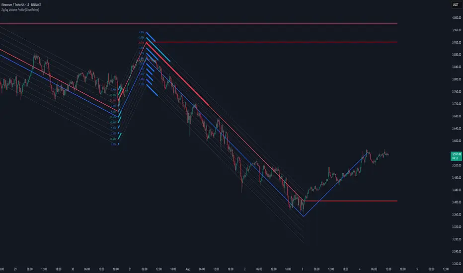
ZigZag Volume Profile [ChartPrime]⯁ OVERVIEW
ZigZag Volume Profile combines swing structure with volume analytics by plotting a ZigZag of major price swings and overlaying a detailed volume profile around each swing. At the end of each swing, it highlights the Point of Control (POC) — the price level with the highest traded volume — and extends it forward to identify key areas of potential support or resistance.
⯁ KEY FEATURES
ZigZag Swing Detection:
Automatically detects swing highs and lows based on a user-defined length, creating clean visual segments of market structure.
These segments act as boundaries for volume profile calculations.
swingHigh = ta.highest(swingLength)
swingLow = ta.lowest(swingLength)
ZigZag Channel Visualization:
The ZigZag structure is connected with sloped lines, forming a visual “channel” of the price movement.
The ZigZag can optionally, scaled by ATR.
Volume Profile Around Each Swing:
For every completed swing (high to low or low to high), the indicator constructs a full volume profile using user-defined bin counts.
It scans volume across price levels in the swing and plots histogram-style bins using a gradient color to indicate volume magnitude.
Dynamic Bin Width and Slope Adjustment:
Bins are distributed across a vertical ATR-based range, and their width is adjusted based on the percentage of total swing volume.
The volume fill direction is adapted to the swing’s slope for visually aligned plotting.
POC Detection and Extension:
The highest volume bin in each swing is identified as the Point of Control (POC).
This level is plotted with a thicker line and extended horizontally into the future as a key reaction level.
Automatic POC Expiry on Price Interaction:
POC lines are continuously extended unless breached by price.
When price crosses the POC level, the extension is terminated — signaling that the level may have been absorbed.
Clean Volume Bin Visualization:
Bin colors range from green (low volume) to blue (higher volume), with the POC always marked in red by default for easy identification.
Volume percentages are optionally labeled at each bin level.
Flexible Swing Profile Parameters:
Users can control:
Number of volume bins
Bin width
Channel width (ATR factor)
Visibility of the swing channel or POC lines
Efficient Memory Handling:
Old POC lines and volume profiles are automatically removed from memory after a threshold to keep charts clean and performant.
⯁ USAGE
Use ZigZag swings to define market structure visually.
Analyze volume profile around each swing to understand where most trading activity occurred.
Use POC extensions as dynamic support/resistance zones for entries, stops, or take-profits.
Watch for price interaction with extended POC lines — breaks may suggest absorbed liquidity or breakout potential.
Use the ATR-based channel width to adapt profiles based on market volatility.
⯁ CONCLUSION
ZigZag Volume Profile offers a powerful fusion of structure and volume. By plotting detailed volume profiles over each price swing and extending the POC as actionable S/R levels, this tool provides deep insight into market participation zones — giving traders a tactical edge in both ranging and trending environments.
Hann Window FIR Filter Ribbon [BigBeluga]🔵 OVERVIEW
The Hann Window FIR Filter Ribbon is a trend-following visualization tool based on a family of FIR filters using the Hann window function. It plots a smooth and dynamic ribbon formed by six Hann filters of progressively increasing length. Gradient coloring and filled bands reveal trend direction and compression/expansion behavior. When short-term trend shifts occur (via filter crossover), it automatically anchors visual support/resistance zones at the nearest swing highs or lows.
🔵 CONCEPTS
Hann FIR Filter: A finite impulse response filter that uses a Hann (cosine-based) window for weighting past price values, resulting in a non-lag, ultra-smooth output.
hannFilter(length)=>
var float hann = na // Final filter output
float filt = 0
float coef = 0
for i = 1 to length
weight = 1 - math.cos(2 * math.pi * i / (length + 1))
filt += price * weight
coef += weight
hann := coef != 0 ? filt / coef : na
Ribbon Stack: The indicator plots 6 Hann FIR filters with increasing lengths, creating a smooth "ribbon" that adapts to price shifts and visually encodes volatility.
Gradient Coloring: Line colors and fill opacity between layers are dynamically adjusted based on the distance between the filters, showing momentum expansion or contraction.
Dynamic Swing Zones: When the shortest filter crosses its nearest neighbor, a swing high/low is located, and a triangle-style level is anchored and projected to the right.
Self-Extending Levels: These dynamic levels persist and extend until invalidated or replaced by a new opposite trend break.
🔵 FEATURES
Plots 6 Hann FIR filters with increasing lengths (controlled by Ribbon Size input).
Automatically colors each filter and the fill between them with smooth gradient transitions.
Detects trend shifts via filter crossover and anchors visual resistance (red) or support (green) zones.
Support/resistance zones are triangle-style bands built around recent swing highs/lows.
Levels auto-extend right and adapt in real time until invalidated by price action.
Ribbon responds smoothly to price and shows contraction or expansion behavior clearly.
No lag in crossover detection thanks to FIR architecture.
Adjustable sensitivity via Length and Ribbon Size inputs.
🔵 HOW TO USE
Use the ribbon gradient as a visual trend strength and smooth direction cue.
Watch for crossover of shortest filters as early trend change signals.
Monitor support/resistance zones as potential high-probability reaction points.
Combine with other tools like momentum or volume to confirm trend breaks.
Adjust ribbon thickness and length to suit your trading timeframe and volatility preference.
🔵 CONCLUSION
Hann Window FIR Filter Ribbon blends digital signal processing with trading logic to deliver a visually refined, non-lagging trend tool. The adaptive ribbon offers insight into momentum compression and release, while swing-based levels give structure to potential reversals. Ideal for traders who seek smooth trend detection with intelligent, auto-adaptive zone plotting.

ZZ++ UltraAlgo Edition v2This updated script builds on the original work by Dev Lucem and introduces visual UltraBuy and UltraShort signals to help identify sharp trend reversals based on real-time pivot highs and lows.
🔑 Features include:
• Smart detection of V-shaped reversals
• Clear labels for actionable swing points
• Optional ZigZag line overlays and trend-based background coloring
• Real-time alerts for buy/sell reversals
• Fully customizable visual settings for traders of all styles
Unlike traditional lagging tools, this version avoids repainting and is designed with simplicity and trend clarity in mind. Perfect for those looking to highlight key turning points without overwhelming the chart.
For advanced, non-lagging indicators supported by backtesting and algorithmic workflows, check out UltraAlgo.com

PulseWave Strategy Markking77PulseWave Strategy (Markking77) — Description & Indicator Roadmap
PulseWave Strategy (Markking77) is a sleek, straightforward trading system that fuses three powerful market indicators — VWAP, MACD, and RSI — into one harmonious tool. Designed for traders who want clear, actionable signals, this strategy captures trend direction, momentum shifts, and market strength to help you spot optimal entry and exit points.
Step 1: VWAP — The Market Trend Compass (Color: Blue)
What it does:
The Volume Weighted Average Price (VWAP) is the average price a security has traded at throughout the day, weighted by volume. It acts as a dynamic benchmark that many institutional traders rely on.
Why it matters:
Price above the VWAP (blue line) signals bullish momentum — buyers dominate.
Price below the VWAP signals bearish momentum — sellers in control.
PulseWave use:
VWAP sets the trend foundation — we trade in the direction the price sits relative to VWAP.
Step 2: MACD — Momentum Confirmation (Colors: Orange & Blue)
What it does:
MACD tracks momentum by comparing short-term and long-term moving averages, using the MACD line and a signal line to indicate shifts.
Why it matters:
When the MACD line (orange) crosses above the Signal line (blue), it signals rising momentum — a bullish cue.
When the MACD line crosses below the signal line, it signals weakening momentum — bearish cue.
PulseWave use:
MACD confirms momentum that aligns with the VWAP trend before entering trades.
Step 3: RSI — The Strength Filter (Color: Purple)
What it does:
The Relative Strength Index (RSI) measures how fast prices are changing to indicate overbought or oversold conditions.
Why it matters:
RSI above 70 = overbought (possible reversal or pause).
RSI below 30 = oversold (potential bounce).
PulseWave use:
RSI filters out trades taken at extreme price levels, avoiding entries that are too stretched.
Color-Coded Roadmap Summary:
Step Indicator Role Buy Signal Sell Signal Color
1 VWAP Trend Direction Price > VWAP (bullish) Price < VWAP (bearish) Blue
2 MACD Momentum Confirmation MACD line crosses above Signal line MACD line crosses below Signal line Orange & Blue
3 RSI Entry Filter RSI < 70 (not overbought) RSI > 30 (not oversold) Purple
How PulseWave Strategy Works:
Buy when price sits above VWAP, MACD line crosses above the Signal line, and RSI is below 70.
Sell (exit) when price drops below VWAP, MACD line crosses below the Signal line, and RSI is above 30.
This layered approach ensures you only trade when trend, momentum, and strength align — reducing false signals and improving your edge.
Why Use PulseWave Strategy?
Clear & Simple: No guesswork — clear color-coded signals guide your decisions.
Robust: Combines trend, momentum, and strength in one system.
Versatile: Fits day trading and swing trading styles alike.
Visual: Easily interpreted signals with minimal clutter.
Crypto Options Greeks & Volatility Analyzer [BackQuant]Crypto Options Greeks & Volatility Analyzer
Overview
The Crypto Options Greeks & Volatility Analyzer is a comprehensive analytical tool that calculates Black-Scholes option Greeks up to the third order for Bitcoin and Ethereum options. It integrates implied volatility data from VOLMEX indices and provides multiple visualization layers for options risk analysis.
Quick Introduction to Options Trading
Options are financial derivatives that give the holder the right, but not the obligation, to buy or sell an underlying asset at a predetermined price (strike price) within a specific time period (expiration date). Understanding options requires grasping two fundamental concepts:
Call Options : Give the right to buy the underlying asset at the strike price. Calls increase in value when the underlying price rises above the strike price.
Put Options : Give the right to sell the underlying asset at the strike price. Puts increase in value when the underlying price falls below the strike price.
The Language of Options: Greeks
Options traders use "Greeks" - mathematical measures that describe how an option's price changes in response to various factors:
Delta : How much the option price moves for each $1 change in the underlying
Gamma : How fast delta changes as the underlying moves
Theta : Daily time decay - how much value erodes each day
Vega : Sensitivity to implied volatility changes
Rho : Sensitivity to interest rate changes
These Greeks are essential for understanding risk. Just as a pilot needs instruments to fly safely, options traders need Greeks to navigate market conditions and manage positions effectively.
Why Volatility Matters
Implied volatility (IV) represents the market's expectation of future price movement. High IV means:
Options are more expensive (higher premiums)
Market expects larger price swings
Better for option sellers
Low IV means:
Options are cheaper
Market expects smaller moves
Better for option buyers
This indicator helps you visualize and quantify these critical concepts in real-time.
Back to the Indicator
Key Features & Components
1. Complete Greeks Calculations
The indicator computes all standard Greeks using the Black-Scholes-Merton model adapted for cryptocurrency markets:
First Order Greeks:
Delta (Δ) : Measures the rate of change of option price with respect to underlying price movement. Ranges from 0 to 1 for calls and -1 to 0 for puts.
Vega (ν) : Sensitivity to implied volatility changes, expressed as price change per 1% change in IV.
Theta (Θ) : Time decay measured in dollars per day, showing how much value erodes with each passing day.
Rho (ρ) : Interest rate sensitivity, measuring price change per 1% change in risk-free rate.
Second Order Greeks:
Gamma (Γ) : Rate of change of delta with respect to underlying price, indicating how quickly delta will change.
Vanna : Cross-derivative measuring delta's sensitivity to volatility changes and vega's sensitivity to price changes.
Charm : Delta decay over time, showing how delta changes as expiration approaches.
Vomma (Volga) : Vega's sensitivity to volatility changes, important for volatility trading strategies.
Third Order Greeks:
Speed : Rate of change of gamma with respect to underlying price (∂Γ/∂S).
Zomma : Gamma's sensitivity to volatility changes (∂Γ/∂σ).
Color : Gamma decay over time (∂Γ/∂T).
Ultima : Third-order volatility sensitivity (∂²ν/∂σ²).
2. Implied Volatility Analysis
The indicator includes a sophisticated IV ranking system that analyzes current implied volatility relative to its recent history:
IV Rank : Percentile ranking of current IV within its 30-day range (0-100%)
IV Percentile : Percentage of days in the lookback period where IV was lower than current
IV Regime Classification : Very Low, Low, High, or Very High
Color-Coded Headers : Visual indication of volatility regime in the Greeks table
Trading regime suggestions based on IV rank:
IV Rank > 75%: "Favor selling options" (high premium environment)
IV Rank 50-75%: "Neutral / Sell spreads"
IV Rank 25-50%: "Neutral / Buy spreads"
IV Rank < 25%: "Favor buying options" (low premium environment)
3. Gamma Zones Visualization
Gamma zones display horizontal price levels where gamma exposure is highest:
Purple horizontal lines indicate gamma concentration areas
Opacity scaling : Darker shading represents higher gamma values
Percentage labels : Shows gamma intensity relative to ATM gamma
Customizable zones : 3-10 price levels can be analyzed
These zones are critical for understanding:
Pin risk around expiration
Potential for explosive price movements
Optimal strike selection for gamma trading
Market maker hedging flows
4. Probability Cones (Expected Move)
The probability cones project expected price ranges based on current implied volatility:
1 Standard Deviation (68% probability) : Shown with dashed green/red lines
2 Standard Deviations (95% probability) : Shown with dotted green/red lines
Time-scaled projection : Cones widen as expiration approaches
Lognormal distribution : Accounts for positive skew in asset prices
Applications:
Strike selection for credit spreads
Identifying high-probability profit zones
Setting realistic price targets
Risk management for undefined risk strategies
5. Breakeven Analysis
The indicator plots key price levels for options positions:
White line : Strike price
Green line : Call breakeven (Strike + Premium)
Red line : Put breakeven (Strike - Premium)
These levels update dynamically as option premiums change with market conditions.
6. Payoff Structure Visualization
Optional P&L labels display profit/loss at expiration for various price levels:
Shows P&L at -2 sigma, -1 sigma, ATM, +1 sigma, and +2 sigma price levels
Separate calculations for calls and puts
Helps visualize option payoff diagrams directly on the chart
Updates based on current option premiums
Configuration Options
Calculation Parameters
Asset Selection : BTC or ETH (limited by VOLMEX IV data availability)
Expiry Options : 1D, 7D, 14D, 30D, 60D, 90D, 180D
Strike Mode : ATM (uses current spot) or Custom (manual strike input)
Risk-Free Rate : Adjustable annual rate for discounting calculations
Display Settings
Greeks Display : Toggle first, second, and third-order Greeks independently
Visual Elements : Enable/disable probability cones, gamma zones, P&L labels
Table Customization : Position (6 options) and text size (4 sizes)
Price Levels : Show/hide strike and breakeven lines
Technical Implementation
Data Sources
Spot Prices : INDEX:BTCUSD and INDEX:ETHUSD for underlying prices
Implied Volatility : VOLMEX:BVIV (Bitcoin) and VOLMEX:EVIV (Ethereum) indices
Real-Time Updates : All calculations update with each price tick
Mathematical Framework
The indicator implements the full Black-Scholes-Merton model:
Standard normal distribution approximations using Abramowitz and Stegun method
Proper annualization factors (365-day year)
Continuous compounding for interest rate calculations
Lognormal price distribution assumptions
Alert Conditions
Four categories of automated alerts:
Price-Based : Underlying crossing strike price
Gamma-Based : 50% surge detection for explosive moves
Moneyness : Deep ITM alerts when |delta| > 0.9
Time/Volatility : Near expiration and vega spike warnings
Practical Applications
For Options Traders
Monitor all Greeks in real-time for active positions
Identify optimal entry/exit points using IV rank
Visualize risk through probability cones and gamma zones
Track time decay and plan rolls
For Volatility Traders
Compare IV across different expiries
Identify mean reversion opportunities
Monitor vega exposure across strikes
Track higher-order volatility sensitivities
Conclusion
The Crypto Options Greeks & Volatility Analyzer transforms complex mathematical models into actionable visual insights. By combining institutional-grade Greeks calculations with intuitive overlays like probability cones and gamma zones, it bridges the gap between theoretical options knowledge and practical trading application.
Whether you're:
A directional trader using options for leverage
A volatility trader capturing IV mean reversion
A hedger managing portfolio risk
Or simply learning about options mechanics
This tool provides the quantitative foundation needed for informed decision-making in cryptocurrency options markets.
Remember that options trading involves substantial risk and complexity. The Greeks and visualizations provided by this indicator are tools for analysis - they should be combined with proper risk management, position sizing, and a thorough understanding of options strategies.
As crypto options markets continue to mature and grow, having professional-grade analytics becomes increasingly important. This indicator ensures you're equipped with the same analytical capabilities used by institutional traders, adapted specifically for the unique characteristics of 24/7 cryptocurrency markets.

ZigZag++ UltraAlgo EditionThis updated script builds on the original work by Dev Lucem and introduces visual UltraBuy and UltraShort signals to help identify sharp trend reversals based on real-time pivot highs and lows.
🔑 Features include:
• Smart detection of V-shaped reversals
• Clear labels for actionable swing points
• Optional ZigZag line overlays and trend-based background coloring
• Real-time alerts for buy/sell reversals
• Fully customizable visual settings for traders of all styles
Unlike traditional lagging tools, this version avoids repainting and is designed with simplicity and trend clarity in mind. Perfect for those looking to highlight key turning points without overwhelming the chart.
For advanced, non-lagging indicators supported by backtesting and algorithmic workflows, check out UltraAlgo.com

Dark Pool Block Trades - Institutional Volume📊 Dark Pool Block Trades - Institutional Volume
Visualize where institutional money positions before major price moves occur. This indicator reveals hidden dark pool block trades that often precede significant price movements - because when smart money deploys millions and billions in strategic accumulation or distribution, retail traders need to see where it's happening.
🎯 WHY DARK POOL DATA MATTERS:
Institutions don't move large capital randomly. Dark pool block trades represent strategic positioning by sophisticated money managers with superior research and conviction. These trades create hidden support/resistance levels that often predict future price action.
The key principle: Follow institutional flow, don't fight it. When institutions get involved, they create high-probability trading opportunities.
💰 HOW INSTITUTIONS INFLUENCE PRICE:
- Large block trades establish hidden accumulation/distribution zones
- Smart money builds positions BEFORE retail awareness increases
- Institutional activity creates "footprints" at key technical levels
- These trades often signal conviction plays ahead of major moves
- Institutions typically add to winning positions throughout trends
🔍 WHAT THIS INDICATOR SHOWS:
- Visual overlay of dark pool block trades directly on price charts
- Track institutional positioning across major stocks and ETFs
- Identify accumulation/distribution zones before they become obvious to retail
- Spot high-conviction institutional trades in real-time visualization
- Customizable block trade size filters and timeframe selection
- Historical institutional activity up to 5 years or custom ranges
💡 THE TRADING ADVANTAGE:
Instead of guessing price direction, see where institutions are already positioning. When large block trades appear in dark pools, you're witnessing strategic institutional commitment that frequently leads to significant price movements.
⚡ HOW IT WORKS:
This Pine Script displays institutional dark pool transactions as visual markers on your charts. The script comes with sample data for immediate use. For expanded ticker coverage and real-time updates, external data services are available.
🎯 IDEAL FOR:
- Swing traders following institutional footprints
- Traders seeking setups backed by smart money conviction
- Position traders looking for accumulation zones
- Anyone wanting to align with institutional flow rather than fight it
🔄 SAMPLE DATA INCLUDED:
Pre-loaded with institutional activity data across popular tickers, updated daily to demonstrate how dark pool activity correlates with future price movements.
The script initially covers these tickers going back 6 months showing the top 10 trades by volume over 400,000 shares: AAPL, AMD, AMZN, ARKK, ARKW, BAC, BITO, COIN, COST, DIA, ETHA, GLD, GOOGL, HD, HYG, IBB, IWM, JNJ, JPM, LQD, MA, META, MSFT, NVDA, PG, QQQ, RIOT, SLV, SMCI, SMH, SOXX, SPY, TLT, TSLA, UNH, USO, V, VEA, VNQ, VOO, VTI, VWO, WMT, XLE, XLF, XLK, XLU, XLV, XLY

Hurst Exponent Adaptive Filter (HEAF) [PhenLabs]📊 PhenLabs - Hurst Exponent Adaptive Filter (HEAF)
Version: PineScript™ v6
📌 Description
The Hurst Exponent Adaptive Filter (HEAF) is an advanced Pine Script indicator designed to dynamically adjust moving average calculations based on real time market regimes detected through the Hurst Exponent. The intention behind the creation of this indicator was not a buy/sell indicator but rather a tool to help sharpen traders ability to distinguish regimes in the market mathematically rather than guessing. By analyzing price persistence, it identifies whether the market is trending, mean-reverting, or exhibiting random walk behavior, automatically adapting the MA length to provide more responsive alerts in volatile conditions and smoother outputs in stable ones. This helps traders avoid false signals in choppy markets and capitalize on strong trends, making it ideal for adaptive trading strategies across various timeframes and assets.
Unlike traditional moving averages, HEAF incorporates fractal dimension analysis via the Hurst Exponent to create a self-tuning filter that evolves with market conditions. Traders benefit from visual cues like color coded regimes, adaptive bands for volatility channels, and an information panel that suggests appropriate strategies, enhancing decision making without constant manual adjustments by the user.
🚀 Points of Innovation
Dynamic MA length adjustment using Hurst Exponent for regime-aware filtering, reducing lag in trends and noise in ranges.
Integrated market regime classification (trending, mean-reverting, random) with visual and alert-based notifications.
Customizable color themes and adaptive bands that incorporate ATR for volatility-adjusted channels.
Built-in information panel providing real-time strategy recommendations based on detected regimes.
Power sensitivity parameter to fine-tune adaptation aggressiveness, allowing personalization for different trading styles.
Support for multiple MA types (EMA, SMA, WMA) within an adaptive framework.
🔧 Core Components
Hurst Exponent Calculation: Computes the fractal dimension of price series over a user-defined lookback to detect market persistence or anti-persistence.
Adaptive Length Mechanism: Maps Hurst values to MA lengths between minimum and maximum bounds, using a power function for sensitivity control.
Moving Average Engine: Applies the chosen MA type (EMA, SMA, or WMA) to the adaptive length for the core filter line.
Adaptive Bands: Creates upper and lower channels using ATR multiplied by a band factor, scaled to the current adaptive length.
Regime Detection: Classifies market state with thresholds (e.g., >0.55 for trending) and triggers alerts on regime changes.
Visualization System: Includes gradient fills, regime-colored MA lines, and an info panel for at-a-glance insights.
🔥 Key Features
Regime-Adaptive Filtering: Automatically shortens MA in mean-reverting markets for quick responses and lengthens it in trends for smoother signals, helping traders stay aligned with market dynamics.
Custom Alerts: Notifies on regime shifts and band breakouts, enabling timely strategy adjustments like switching to trend-following in bullish regimes.
Visual Enhancements: Color-coded MA lines, gradient band fills, and an optional info panel that displays market state and trading tips, improving chart readability.
Flexible Settings: Adjustable lookback, min/max lengths, sensitivity power, MA type, and themes to suit various assets and timeframes.
Band Breakout Signals: Highlights potential overbought/oversold conditions via ATR-based channels, useful for entry/exit timing.
🎨 Visualization
Main Adaptive MA Line: Plotted with regime-based colors (e.g., green for trending) to visually indicate market state and filter position relative to price.
Adaptive Bands: Upper and lower lines with gradient fills between them, showing volatility channels that widen in random regimes and tighten in trends.
Price vs. MA Fills: Color-coded areas between price and MA (e.g., bullish green above MA in trending modes) for quick trend strength assessment.
Information Panel: Top-right table displaying current regime (e.g., "Trending Market") and strategy suggestions like "Follow trends" or "Trade ranges."
📖 Usage Guidelines
Core Settings
Hurst Lookback Period
Default: 100
Range: 20-500
Description: Sets the period for Hurst Exponent calculation; longer values provide more stable regime detection but may lag, while shorter ones are more responsive to recent changes.
Minimum MA Length
Default: 10
Range: 5-50
Description: Defines the shortest possible adaptive MA length, ideal for fast responses in mean-reverting conditions.
Maximum MA Length
Default: 200
Range: 50-500
Description: Sets the longest adaptive MA length for smoothing in strong trends; adjust based on asset volatility.
Sensitivity Power
Default: 2.0
Range: 1.0-5.0
Description: Controls how aggressively the length adapts to Hurst changes; higher values make it more sensitive to regime shifts.
MA Type
Default: EMA
Options: EMA, SMA, WMA
Description: Chooses the moving average calculation method; EMA is more responsive, while SMA/WMA offer different weighting.
🖼️ Visual Settings
Show Adaptive Bands
Default: True
Description: Toggles visibility of upper/lower bands for volatility channels.
Band Multiplier
Default: 1.5
Range: 0.5-3.0
Description: Scales band width using ATR; higher values create wider channels for conservative signals.
Show Information Panel
Default: True
Description: Displays regime info and strategy tips in a top-right panel.
MA Line Width
Default: 2
Range: 1-5
Description: Adjusts thickness of the main MA line for better visibility.
Color Theme
Default: Blue
Options: Blue, Classic, Dark Purple, Vibrant
Description: Selects color scheme for MA, bands, and fills to match user preferences.
🚨 Alert Settings
Enable Alerts
Default: True
Description: Activates notifications for regime changes and band breakouts.
✅ Best Use Cases
Trend-Following Strategies: In detected trending regimes, use the adaptive MA as a trailing stop or entry filter for momentum trades.
Range Trading: During mean-reverting periods, monitor band breakouts for buying dips or selling rallies within channels.
Risk Management in Random Markets: Reduce exposure when random walk is detected, using tight stops suggested in the info panel.
Multi-Timeframe Analysis: Apply on higher timeframes for regime confirmation, then drill down to lower ones for entries.
Volatility-Based Entries: Use upper/lower band crossovers as signals in adaptive channels for overbought/oversold trades.
⚠️ Limitations
Lagging in Transitions: Regime detection may delay during rapid market shifts, requiring confirmation from other tools.
Not a Standalone System: Best used in conjunction with other indicators; random regimes can lead to whipsaws if traded aggressively.
Parameter Sensitivity: Optimal settings vary by asset and timeframe, necessitating backtesting.
💡 What Makes This Unique
Hurst-Driven Adaptation: Unlike static MAs, it uses fractal analysis to self-tune, providing regime-specific filtering that's rare in standard indicators.
Integrated Strategy Guidance: The info panel offers actionable tips tied to regimes, bridging analysis and execution.
Multi-Regime Visualization: Combines adaptive bands, colored fills, and alerts in one tool for comprehensive market state awareness.
🔬 How It Works
Hurst Exponent Computation:
Calculates log returns over the lookback period to derive the rescaled range (R/S) ratio.
Normalizes to a 0-1 value, where >0.55 indicates trending, <0.45 mean-reverting, and in-between random.
Length Adaptation:
Maps normalized Hurst to an MA length via a power function, clamping between min and max.
Applies the selected MA type to close prices using this dynamic length.
Visualization and Signals:
Plots the MA with regime colors, adds ATR-based bands, and fills areas for trend strength.
Triggers alerts on regime changes or band crosses, with the info panel suggesting strategies like momentum riding in trends.
💡 Note:
For optimal results, backtest settings on your preferred assets and combine with volume or momentum indicators. Remember, no indicator guarantees profits—use with proper risk management. Access premium features and support at PhenLabs.

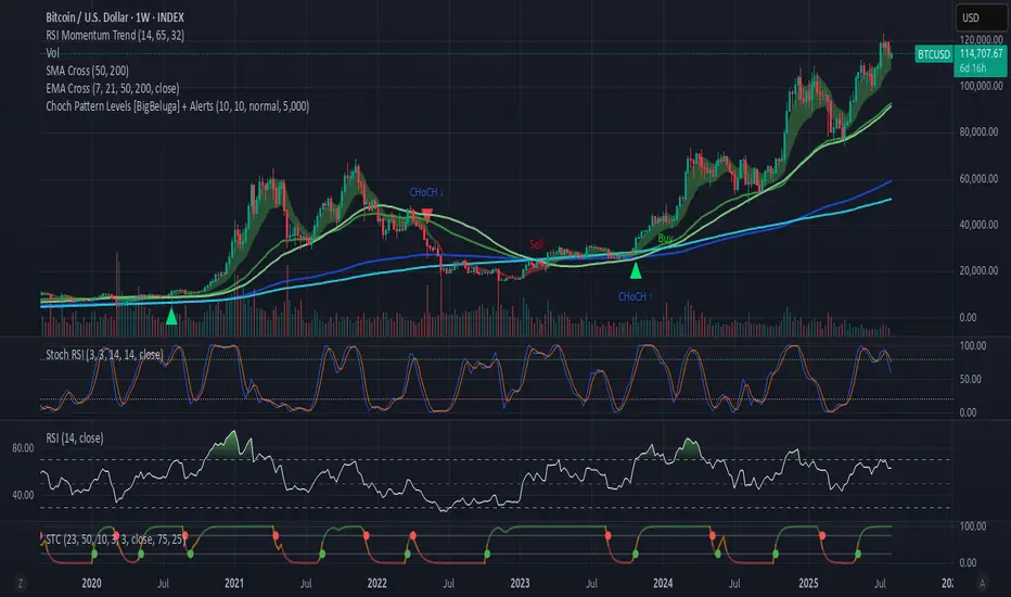
Choch Pattern Levels [BigBeluga] + AlertsChoch Pattern Levels highlights key structural breaks that can mark the start of new trends. By combining precise break detection with volume analytics and automatic cleanup, it provides actionable insights into the true intent behind price moves — giving traders a clean edge in spotting early reversals and key reaction zones. Added support for alarms.
Volume Pressure Gauge + Volume %Volume Pressure Gauge and Volume Percentage Indicator – Pine Script Guide
This indicator provides a simplified, real-time visualization of both volume pressure (buy vs. sell activity) and today’s trading volume in comparison to historical averages. It is designed to help traders assess whether buyers or sellers dominate the current session and whether today’s volume is significant relative to recent behaviour.
________________________________________
Key Functional Segments
1. Inputs and Configuration
Users can configure the length of the Simple Moving Average (SMA) used to calculate average volume, set the position of the gauge table on the chart, and toggle the visibility of the volume pressure display. This allows flexibility in integrating the tool with various trading styles and chart layouts.
2. Volume Data Calculations
The indicator calculates three key volume metrics:
• volToday: The current day’s volume.
• volAvg: The average volume over the user-defined SMA period (default is 20 bars).
• volPct: The current volume as a percentage of the average.
This enables traders to quickly recognize whether current trading activity is above or below normal, which can be a precursor to potential trend strength or weakness.
3. Volume Pressure Calculation
The script estimates buying and selling pressure based on price movement and volume. It distributes volume into upward (buy) and downward (sell) segments and expresses them as percentages of the total volume. This gives an immediate sense of whether bulls or bears are more active in the current session.
4. Visual Representation (Progress Bars)
The indicator renders a simplified visual gauge using horizontal bar segments (pseudo-bars) to reflect the proportion of buy and sell pressure. The length of each bar correlates with the strength of pressure from buyers or sellers, helping users assess dominance without analyzing candlestick behavior in depth.
5. Table Display
A compact table is drawn on the chart showing:
• Buy pressure percentage and corresponding bar.
• Sell pressure percentage and corresponding bar.
• Volume percentage compared to the recent average.
This format makes it easy to evaluate volume dynamics at a glance, without cluttering the price chart or relying on separate overlays.
________________________________________
How Traders Benefit from This Indicator
• Momentum Shift Detection: Early signs of trend reversal can be observed when volume pressure flips direction.
• Breakout Validation: High volume combined with dominant pressure supports the credibility of breakout moves.
• False Move Avoidance: If price moves on low volume or mixed pressure, traders can avoid low-probability entries.
• Market Context Awareness: Users can assess whether a day is behaving normally in terms of participation or is unusually quiet or aggressive.
________________________________________
Basic Usage Guide
1. Add the script to your TradingView chart and set your preferred SMA length for volume comparison.
2. Customize the table’s position using the X and Y settings for clarity and alignment.
3. Interpret the outputs:
o A higher red bar indicates dominant sell pressure.
o A higher green bar indicates dominant buy pressure.
o Volume % above 100% suggests above-average activity, while values below 100% may imply low conviction.
4. Apply to trading decisions:
o High buy pressure and high volume may indicate a strong long opportunity.
o High sell pressure and high volume may support short setups.
o Low volume or conflicting signals may call for caution.
5. Combine with other tools such as trend indicators, support/resistance zones, or price action patterns for more reliable trade setups.
________________________________________
Practical Example
• Sell Pressure: 70% → Suggests strong seller control; potential for short setups.
• Buy Pressure: 30% → Weak buying interest; long trades may carry risk.
• Volume Percentage: 120% → Indicates a surge in participation; movement may have greater validity.
________________________________________
Tips for New Traders
• Use this indicator as a confirmation tool rather than a standalone strategy.
• Begin on higher timeframes (4-hour or daily) to develop familiarity.
• Compare multiple examples to identify reliable patterns over time.
• Always incorporate proper risk management, including stop losses.
________________________________________
Disclaimer from aiTrendview
This indicator is intended solely for educational and informational use. It does not constitute investment advice, trade signals, or financial recommendations. aiTrendview and its affiliates are not liable for any trading losses incurred through use of this tool. All trading involves risk. Past performance of any indicator does not guarantee future results. Users should conduct independent research and consult with a certified financial advisor before making any trading decisions.

Time-Decaying Percentile Oscillator [BackQuant]Time-Decaying Percentile Oscillator
1. Big-picture idea
Traditional percentile or stochastic oscillators treat every bar in the look-back window as equally important. That is fine when markets are slow, but if volatility regime changes quickly yesterday’s print should matter more than last month’s. The Time-Decaying Percentile Oscillator attempts to fix that blind spot by assigning an adjustable weight to every past price before it is ranked. The result is a percentile score that “breathes” with market tempo much faster to flag new extremes yet still smooth enough to ignore random noise.
2. What the script actually does
Build a weight curve
• You pick a look-back length (default 28 bars).
• You decide whether weights fall Linearly , Exponentially , by Power-law or Logarithmically .
• A decay factor (lower = faster fade) shapes how quickly the oldest price loses influence.
• The array is normalised so all weights still sum to 1.
Rank prices by weighted mass
• Every close in the window is paired with its weight.
• The pairs are sorted from low to high.
• The cumulative weight is walked until it equals your chosen percentile level (default 50 = median).
• That price becomes the Time-Decayed Percentile .
Find dispersion with robust statistics
• Instead of a fragile standard deviation the script measures weighted Median-Absolute-Deviation about the new percentile.
• You multiply that deviation by the Deviation Multiplier slider (default 1.0) to get a non-parametric volatility band.
Build an adaptive channel
• Upper band = percentile + (multiplier × deviation)
• Lower band = percentile – (multiplier × deviation)
Normalise into a 0-100 oscillator
• The current close is mapped inside that band:
0 = lower band, 50 = centre, 100 = upper band.
• If the channel squeezes, tiny moves still travel the full scale; if volatility explodes, it automatically widens.
Optional smoothing
• A second-stage moving average (EMA, SMA, DEMA, TEMA, etc.) tames the jitter.
• Length 22 EMA by default—change it to tune reaction speed.
Threshold logic
• Upper Threshold 70 and Lower Threshold 30 separate standard overbought/oversold states.
• Extreme bands 85 and 15 paint background heat when aggressive fade or breakout trades might trigger.
Divergence engine
• Looks back twenty bars.
• Flags Bullish divergence when price makes a lower low but oscillator refuses to confirm (value < 40).
• Flags Bearish divergence when price prints a higher high but oscillator stalls (value > 60).
3. Component walk-through
• Source – Any price series. Close by default, switch to typical price or custom OHLC4 for futures spreads.
• Look-back Period – How many bars to rank. Short = faster, long = slower.
• Base Percentile Level – 50 shows relative position around the median; set to 25 / 75 for quartile tracking or 90 / 10 for extreme tails.
• Deviation Multiplier – Higher values widen the dynamic channel, lowering whipsaw but delaying signals.
• Decay Settings
– Type decides the curve shape. Exponential (default 1.16) mimics EMA logic.
– Factor < 1 shrinks influence faster; > 1 spreads influence flatter.
– Toggle Enable Time Decay off to compare with classic equal-weight stochastic.
• Smoothing Block – Choose one of seven MA flavours plus length.
• Thresholds – Overbought / Oversold / Extreme levels. Push them out when working on very mean-reverting assets like FX; pull them in for trend monsters like crypto.
• Display toggles – Show or hide threshold lines, extreme filler zones, bar colouring, divergence labels.
• Colours – Bullish green, bearish red, neutral grey. Every gradient step is automatically blended to generate a heat map across the 0-100 range.
4. How to read the chart
• Oscillator creeping above 70 = market auctioning near the top of its adaptive range.
• Fast poke above 85 with no follow-through = exhaustion fade candidate.
• Slow grind that lives above 70 for many bars = valid bullish trend, not a fade.
• Cross back through 50 shows balance has shifted; treat it like a micro trend change.
• Divergence arrows add extra confidence when you already see two-bar reversal candles at range extremes.
• Background shading (semi-transparent red / green) warns of extreme states and throttles your position size.
5. Practical trading playbook
Mean-reversion scalps
1. Wait for oscillator to reach your desired OB/ OS levels
2. Check the slope of the smoothing MA—if it is flattening the squeeze is mature.
3. Look for a one- or two-bar reversal pattern.
4. Enter against the move; first target = midline 50, second target = opposite threshold.
5. Stop loss just beyond the extreme band.
Trend continuation pullbacks
1. Identify a clean directional trend on the price chart.
2. During the trend, TDP will oscillate between midline and extreme of that side.
3. Buy dips when oscillator hits OS levels, and the same for OB levels & shorting
4. Exit when oscillator re-tags the same-side extreme or prints divergence.
Volatility regime filter
• Use the Enable Time Decay switch as a regime test.
• If equal-weight oscillator and decayed oscillator diverge widely, market is entering a new volatility regime—tighten stops and trade smaller.
Divergence confirmation for other indicators
• Pair TDP divergence arrows with MACD histogram or RSI to filter false positives.
• The weighted nature means TDP often spots divergence a bar or two earlier than standard RSI.
Swing breakout strategy
1. During consolidation, band width compresses and oscillator oscillates around 50.
2. Watch for sudden expansion where oscillator blasts through extreme bands and stays pinned.
3. Enter with momentum in breakout direction; trail stop behind upper or lower band as it re-expands.
6. Customising decay mathematics
Linear – Each older bar loses the same fixed amount of influence. Intuitive and stable; good for slow swing charts.
Exponential – Influence halves every “decay factor” steps. Mirrors EMA thinking and is fastest to react.
Power-law – Mid-history bars keep more authority than exponential but oldest data still fades. Handy for commodities where seasonality matters.
Logarithmic – The gentlest curve; weight drops sharply at first then levels off. Mimics how traders remember dramatic moves for weeks but forget ordinary noise quickly.
Turn decay off to verify the tool’s added value; most users never switch back.
7. Alert catalogue
• TD Overbought / TD Oversold – Cross of regular thresholds.
• TD Extreme OB / OS – Breach of danger zones.
• TD Bullish / Bearish Divergence – High-probability reversal watch.
• TD Midline Cross – Momentum shift that often precedes a window where trend-following systems perform.
8. Visual hygiene tips
• If you already plot price on a dark background pick Bullish Color and Bearish Color default; change to pastel tones for light themes.
• Hide threshold lines after you memorise the zones to declutter scalping layouts.
• Overlay mode set to false so the oscillator lives in its own panel; keep height about 30 % of screen for best resolution.
9. Final notes
Time-Decaying Percentile Oscillator marries robust statistical ranking, adaptive dispersion and decay-aware weighting into a simple oscillator. It respects both recent order-flow shocks and historical context, offers granular control over responsiveness and ships with divergence and alert plumbing out of the box. Bolt it onto your price action framework, trend-following system or volatility mean-reversion playbook and see how much sooner it recognises genuine extremes compared to legacy oscillators.
Backtest thoroughly, experiment with decay curves on each asset class and remember: in trading, timing beats timidity but patience beats impulse. May this tool help you find that edge.

Multi-Timeframe SFP + SMTImportant: Please Read First
This indicator is not a "one size fits all" solution. It is a professional and complex tool that requires you to learn how to use it, in addition to backtesting different settings to discover what works best for your specific trading style and the assets you trade. The default settings provided are my personal preferences for trading higher-timeframe setups, but you are encouraged to experiment and find your own optimal configuration.
Please note that while this initial version is solid, it may still contain small errors or bugs. I will be actively working on improving the indicator over time. Also, be aware that the script is not written for maximum efficiency and may be resource-intensive, but this should not pose a problem for most users.
The source code for this indicator is open. If you truly want to understand precisely how all the logic works, you can copy and paste the code into an AI assistant like Gemini or ChatGPT and ask it to explain any part of the script to you.
Author's Preferred Settings (Guideline)
As a starting point, here are the settings I personally use for my trading:
SFP Timeframe: 4-Hour (Strength: 5-5)
Max Lookback: 35 Bars
Raid Expiration: 1 Bar
SFP Lines Limit: 1
SMT Timeframe 1: 30-Minute (Strength: 2-2) with 3-Minute LTF Detection.
SMT Timeframe 2: 15-Minute (Strength: 3-3) with 3-Minute LTF Detection.
SMT Timeframe 3: 1-Hour (Strength: 1-1) with 3-Minute LTF Detection.
SMT Timeframe 4: 15-Minute (Strength: 1-1) with 3-Minute LTF Detection.
Multi-Timeframe SMT: An Overview
This indicator is a powerful tool designed to identify high-probability trading setups by combining two key institutional concepts: Swing Failure Patterns (SFP) on a higher timeframe and Smart Money Technique (SMT) divergences on a lower timeframe. A key feature is the ability to configure and run up to four independent SMT analyses simultaneously, allowing you to monitor for divergences across multiple timeframes (e.g., 15m, 1H, 4H) from a single indicator.
Its primary purpose is to generate automated signals through TradingView's alert system. By setting up alerts, the script runs server-side, monitoring the market for you. When a setup presents itself, it will send a push notification to your device, allowing you to personally evaluate the trade without being tied to your screen.
The Strategy: HTF Liquidity Sweeps into LTF SMT
The core strategy is built on a classic institutional trading model:
Wait for a liquidity sweep on a significant high timeframe (e.g., 4-hour, Daily).
Once liquidity is taken, look for a confirmation of a shift in market structure on a lower timeframe.
This indicator uses an SMT divergence as that confirmation signal, indicating that smart money may be stepping in to reverse the price.
How It Works: The Two-Step Process
The indicator's logic follows a precise two-step process to generate a signal:
Step 1: The Swing Failure Pattern (SFP)
First, the indicator identifies a high-timeframe liquidity sweep. This is configured in the "Swing Failure Pattern (SFP) Timeframe" settings.
It looks for a candle that wicks above a previous high (or below a previous low) but then closes back within the range of that pivot. This action is known as a "raid" or a "swing failure," suggesting the move failed to find genuine momentum.
Step 2: The SMT Divergence
The moment a valid SFP is confirmed, the indicator's multiple SMT engines activate.
Each engine begins monitoring the specific SMT timeframe you have configured (e.g., "SMT Timeframe 1," "SMT Timeframe 2," etc.) for a Smart Money Technique (SMT) divergence.
An SMT divergence occurs when two closely correlated assets fail to move in sync. For example, after a raid on a high, Asset A makes a new high, but Asset B fails to do so. This disagreement suggests weakness and a potential reversal.
When the script finds this divergence, it plots the SMT line and triggers an alert.
The Power of Alerts
The true strength of this indicator lies in its alert capabilities. You can create alerts for both unconfirmed and confirmed SMTs.
Enable Alerts LTF Detection: These alerts trigger when an unconfirmed, potential SMT is spotted on the lower "LTF Detection" timeframe. While not yet confirmed, these early alerts can notify you of a potential move before it fully happens, allowing you to be ahead of the curve and find the best possible trade entries.
Enable Alerts Confirmed SMT: These alerts trigger only when a permanent, confirmed SMT line is plotted on your chosen SMT timeframe. These signals are more reliable but occur later than the early detection alerts.
Key Concepts Explained
What is Pivot Strength?
Pivot Strength determines how significant a high or low needs to be to qualify as a valid structural point. A setting of 5-5, for example, means that for a candle's high to be considered a valid pivot high, its high must be higher than the highs of the 5 candles to its left and the 5 candles to its right.
Higher Strength (e.g., 5-5, 8-8): Creates fewer, but more significant, pivots. This is ideal for identifying major structural highs and lows on higher timeframes.
Lower Strength (e.g., 2-2, 3-3): Creates more pivots, making it suitable for identifying the smaller shifts in momentum on lower timeframes.
Raid Expiration & Validity
An SFP signal is not valid forever. The "Raid Expiration" setting determines how many SFP timeframe bars can pass after a raid before that signal is considered "stale" and can no longer be used to validate an SMT. This ensures your SMT divergences are always in response to recent liquidity sweeps.
Why You Must Be on the Right Chart Timeframe to See SMT Lines
Pine Script™ has a fundamental rule: an indicator running on a chart can only "see" the bars of that chart's timeframe or higher.
When the SMT logic is set to the 15-minute timeframe, it calculates its pivots based on 15-minute data. To accurately plot lines connecting these pivots, you must be on a 15-minute chart or lower (e.g., 5-minute, 1-minute).
If you are on a higher timeframe chart, like the 1-hour, the 15-minute bars do not exist on that chart, so the indicator has no bars to draw the lines on.
This is precisely why the alert system is so powerful. You can set your alert to run on the 15-minute timeframe, and TradingView's servers will monitor that timeframe for you, sending a notification regardless of what chart you are currently viewing.

Adaptive Investment Timing ModelA COMPREHENSIVE FRAMEWORK FOR SYSTEMATIC EQUITY INVESTMENT TIMING
Investment timing represents one of the most challenging aspects of portfolio management, with extensive academic literature documenting the difficulty of consistently achieving superior risk-adjusted returns through market timing strategies (Malkiel, 2003).
Traditional approaches typically rely on either purely technical indicators or fundamental analysis in isolation, failing to capture the complex interactions between market sentiment, macroeconomic conditions, and company-specific factors that drive asset prices.
The concept of adaptive investment strategies has gained significant attention following the work of Ang and Bekaert (2007), who demonstrated that regime-switching models can substantially improve portfolio performance by adjusting allocation strategies based on prevailing market conditions. Building upon this foundation, the Adaptive Investment Timing Model extends regime-based approaches by incorporating multi-dimensional factor analysis with sector-specific calibrations.
Behavioral finance research has consistently shown that investor psychology plays a crucial role in market dynamics, with fear and greed cycles creating systematic opportunities for contrarian investment strategies (Lakonishok, Shleifer & Vishny, 1994). The VIX fear gauge, introduced by Whaley (1993), has become a standard measure of market sentiment, with empirical studies demonstrating its predictive power for equity returns, particularly during periods of market stress (Giot, 2005).
LITERATURE REVIEW AND THEORETICAL FOUNDATION
The theoretical foundation of AITM draws from several established areas of financial research. Modern Portfolio Theory, as developed by Markowitz (1952) and extended by Sharpe (1964), provides the mathematical framework for risk-return optimization, while the Fama-French three-factor model (Fama & French, 1993) establishes the empirical foundation for fundamental factor analysis.
Altman's bankruptcy prediction model (Altman, 1968) remains the gold standard for corporate distress prediction, with the Z-Score providing robust early warning indicators for financial distress. Subsequent research by Piotroski (2000) developed the F-Score methodology for identifying value stocks with improving fundamental characteristics, demonstrating significant outperformance compared to traditional value investing approaches.
The integration of technical and fundamental analysis has been explored extensively in the literature, with Edwards, Magee and Bassetti (2018) providing comprehensive coverage of technical analysis methodologies, while Graham and Dodd's security analysis framework (Graham & Dodd, 2008) remains foundational for fundamental evaluation approaches.
Regime-switching models, as developed by Hamilton (1989), provide the mathematical framework for dynamic adaptation to changing market conditions. Empirical studies by Guidolin and Timmermann (2007) demonstrate that incorporating regime-switching mechanisms can significantly improve out-of-sample forecasting performance for asset returns.
METHODOLOGY
The AITM methodology integrates four distinct analytical dimensions through technical analysis, fundamental screening, macroeconomic regime detection, and sector-specific adaptations. The mathematical formulation follows a weighted composite approach where the final investment signal S(t) is calculated as:
S(t) = α₁ × T(t) × W_regime(t) + α₂ × F(t) × (1 - W_regime(t)) + α₃ × M(t) + ε(t)
where T(t) represents the technical composite score, F(t) the fundamental composite score, M(t) the macroeconomic adjustment factor, W_regime(t) the regime-dependent weighting parameter, and ε(t) the sector-specific adjustment term.
Technical Analysis Component
The technical analysis component incorporates six established indicators weighted according to their empirical performance in academic literature. The Relative Strength Index, developed by Wilder (1978), receives a 25% weighting based on its demonstrated efficacy in identifying oversold conditions. Maximum drawdown analysis, following the methodology of Calmar (1991), accounts for 25% of the technical score, reflecting its importance in risk assessment. Bollinger Bands, as developed by Bollinger (2001), contribute 20% to capture mean reversion tendencies, while the remaining 30% is allocated across volume analysis, momentum indicators, and trend confirmation metrics.
Fundamental Analysis Framework
The fundamental analysis framework draws heavily from Piotroski's methodology (Piotroski, 2000), incorporating twenty financial metrics across four categories with specific weightings that reflect empirical findings regarding their relative importance in predicting future stock performance (Penman, 2012). Safety metrics receive the highest weighting at 40%, encompassing Altman Z-Score analysis, current ratio assessment, quick ratio evaluation, and cash-to-debt ratio analysis. Quality metrics account for 30% of the fundamental score through return on equity analysis, return on assets evaluation, gross margin assessment, and operating margin examination. Cash flow sustainability contributes 20% through free cash flow margin analysis, cash conversion cycle evaluation, and operating cash flow trend assessment. Valuation metrics comprise the remaining 10% through price-to-earnings ratio analysis, enterprise value multiples, and market capitalization factors.
Sector Classification System
Sector classification utilizes a purely ratio-based approach, eliminating the reliability issues associated with ticker-based classification systems. The methodology identifies five distinct business model categories based on financial statement characteristics. Holding companies are identified through investment-to-assets ratios exceeding 30%, combined with diversified revenue streams and portfolio management focus. Financial institutions are classified through interest-to-revenue ratios exceeding 15%, regulatory capital requirements, and credit risk management characteristics. Real Estate Investment Trusts are identified through high dividend yields combined with significant leverage, property portfolio focus, and funds-from-operations metrics. Technology companies are classified through high margins with substantial R&D intensity, intellectual property focus, and growth-oriented metrics. Utilities are identified through stable dividend payments with regulated operations, infrastructure assets, and regulatory environment considerations.
Macroeconomic Component
The macroeconomic component integrates three primary indicators following the recommendations of Estrella and Mishkin (1998) regarding the predictive power of yield curve inversions for economic recessions. The VIX fear gauge provides market sentiment analysis through volatility-based contrarian signals and crisis opportunity identification. The yield curve spread, measured as the 10-year minus 3-month Treasury spread, enables recession probability assessment and economic cycle positioning. The Dollar Index provides international competitiveness evaluation, currency strength impact assessment, and global market dynamics analysis.
Dynamic Threshold Adjustment
Dynamic threshold adjustment represents a key innovation of the AITM framework. Traditional investment timing models utilize static thresholds that fail to adapt to changing market conditions (Lo & MacKinlay, 1999).
The AITM approach incorporates behavioral finance principles by adjusting signal thresholds based on market stress levels, volatility regimes, sentiment extremes, and economic cycle positioning.
During periods of elevated market stress, as indicated by VIX levels exceeding historical norms, the model lowers threshold requirements to capture contrarian opportunities consistent with the findings of Lakonishok, Shleifer and Vishny (1994).
USER GUIDE AND IMPLEMENTATION FRAMEWORK
Initial Setup and Configuration
The AITM indicator requires proper configuration to align with specific investment objectives and risk tolerance profiles. Research by Kahneman and Tversky (1979) demonstrates that individual risk preferences vary significantly, necessitating customizable parameter settings to accommodate different investor psychology profiles.
Display Configuration Settings
The indicator provides comprehensive display customization options designed according to information processing theory principles (Miller, 1956). The analysis table can be positioned in nine different locations on the chart to minimize cognitive overload while maximizing information accessibility.
Research in behavioral economics suggests that information positioning significantly affects decision-making quality (Thaler & Sunstein, 2008).
Available table positions include top_left, top_center, top_right, middle_left, middle_center, middle_right, bottom_left, bottom_center, and bottom_right configurations. Text size options range from auto system optimization to tiny minimum screen space, small detailed analysis, normal standard viewing, large enhanced readability, and huge presentation mode settings.
Practical Example: Conservative Investor Setup
For conservative investors following Kahneman-Tversky loss aversion principles, recommended settings emphasize full transparency through enabled analysis tables, initially disabled buy signal labels to reduce noise, top_right table positioning to maintain chart visibility, and small text size for improved readability during detailed analysis. Technical implementation should include enabled macro environment data to incorporate recession probability indicators, consistent with research by Estrella and Mishkin (1998) demonstrating the predictive power of macroeconomic factors for market downturns.
Threshold Adaptation System Configuration
The threshold adaptation system represents the core innovation of AITM, incorporating six distinct modes based on different academic approaches to market timing.
Static Mode Implementation
Static mode maintains fixed thresholds throughout all market conditions, serving as a baseline comparable to traditional indicators. Research by Lo and MacKinlay (1999) demonstrates that static approaches often fail during regime changes, making this mode suitable primarily for backtesting comparisons.
Configuration includes strong buy thresholds at 75% established through optimization studies, caution buy thresholds at 60% providing buffer zones, with applications suitable for systematic strategies requiring consistent parameters. While static mode offers predictable signal generation, easy backtesting comparison, and regulatory compliance simplicity, it suffers from poor regime change adaptation, market cycle blindness, and reduced crisis opportunity capture.
Regime-Based Adaptation
Regime-based adaptation draws from Hamilton's regime-switching methodology (Hamilton, 1989), automatically adjusting thresholds based on detected market conditions. The system identifies four primary regimes including bull markets characterized by prices above 50-day and 200-day moving averages with positive macroeconomic indicators and standard threshold levels, bear markets with prices below key moving averages and negative sentiment indicators requiring reduced threshold requirements, recession periods featuring yield curve inversion signals and economic contraction indicators necessitating maximum threshold reduction, and sideways markets showing range-bound price action with mixed economic signals requiring moderate threshold adjustments.
Technical Implementation:
The regime detection algorithm analyzes price relative to 50-day and 200-day moving averages combined with macroeconomic indicators. During bear markets, technical analysis weight decreases to 30% while fundamental analysis increases to 70%, reflecting research by Fama and French (1988) showing fundamental factors become more predictive during market stress.
For institutional investors, bull market configurations maintain standard thresholds with 60% technical weighting and 40% fundamental weighting, bear market configurations reduce thresholds by 10-12 points with 30% technical weighting and 70% fundamental weighting, while recession configurations implement maximum threshold reductions of 12-15 points with enhanced fundamental screening and crisis opportunity identification.
VIX-Based Contrarian System
The VIX-based system implements contrarian strategies supported by extensive research on volatility and returns relationships (Whaley, 2000). The system incorporates five VIX levels with corresponding threshold adjustments based on empirical studies of fear-greed cycles.
Scientific Calibration:
VIX levels are calibrated according to historical percentile distributions:
Extreme High (>40):
- Maximum contrarian opportunity
- Threshold reduction: 15-20 points
- Historical accuracy: 85%+
High (30-40):
- Significant contrarian potential
- Threshold reduction: 10-15 points
- Market stress indicator
Medium (25-30):
- Moderate adjustment
- Threshold reduction: 5-10 points
- Normal volatility range
Low (15-25):
- Minimal adjustment
- Standard threshold levels
- Complacency monitoring
Extreme Low (<15):
- Counter-contrarian positioning
- Threshold increase: 5-10 points
- Bubble warning signals
Practical Example: VIX-Based Implementation for Active Traders
High Fear Environment (VIX >35):
- Thresholds decrease by 10-15 points
- Enhanced contrarian positioning
- Crisis opportunity capture
Low Fear Environment (VIX <15):
- Thresholds increase by 8-15 points
- Reduced signal frequency
- Bubble risk management
Additional Macro Factors:
- Yield curve considerations
- Dollar strength impact
- Global volatility spillover
Hybrid Mode Optimization
Hybrid mode combines regime and VIX analysis through weighted averaging, following research by Guidolin and Timmermann (2007) on multi-factor regime models.
Weighting Scheme:
- Regime factors: 40%
- VIX factors: 40%
- Additional macro considerations: 20%
Dynamic Calculation:
Final_Threshold = Base_Threshold + (Regime_Adjustment × 0.4) + (VIX_Adjustment × 0.4) + (Macro_Adjustment × 0.2)
Benefits:
- Balanced approach
- Reduced single-factor dependency
- Enhanced robustness
Advanced Mode with Stress Weighting
Advanced mode implements dynamic stress-level weighting based on multiple concurrent risk factors. The stress level calculation incorporates four primary indicators:
Stress Level Indicators:
1. Yield curve inversion (recession predictor)
2. Volatility spikes (market disruption)
3. Severe drawdowns (momentum breaks)
4. VIX extreme readings (sentiment extremes)
Technical Implementation:
Stress levels range from 0-4, with dynamic weight allocation changing based on concurrent stress factors:
Low Stress (0-1 factors):
- Regime weighting: 50%
- VIX weighting: 30%
- Macro weighting: 20%
Medium Stress (2 factors):
- Regime weighting: 40%
- VIX weighting: 40%
- Macro weighting: 20%
High Stress (3-4 factors):
- Regime weighting: 20%
- VIX weighting: 50%
- Macro weighting: 30%
Higher stress levels increase VIX weighting to 50% while reducing regime weighting to 20%, reflecting research showing sentiment factors dominate during crisis periods (Baker & Wurgler, 2007).
Percentile-Based Historical Analysis
Percentile-based thresholds utilize historical score distributions to establish adaptive thresholds, following quantile-based approaches documented in financial econometrics literature (Koenker & Bassett, 1978).
Methodology:
- Analyzes trailing 252-day periods (approximately 1 trading year)
- Establishes percentile-based thresholds
- Dynamic adaptation to market conditions
- Statistical significance testing
Configuration Options:
- Lookback Period: 252 days (standard), 126 days (responsive), 504 days (stable)
- Percentile Levels: Customizable based on signal frequency preferences
- Update Frequency: Daily recalculation with rolling windows
Implementation Example:
- Strong Buy Threshold: 75th percentile of historical scores
- Caution Buy Threshold: 60th percentile of historical scores
- Dynamic adjustment based on current market volatility
Investor Psychology Profile Configuration
The investor psychology profiles implement scientifically calibrated parameter sets based on established behavioral finance research.
Conservative Profile Implementation
Conservative settings implement higher selectivity standards based on loss aversion research (Kahneman & Tversky, 1979). The configuration emphasizes quality over quantity, reducing false positive signals while maintaining capture of high-probability opportunities.
Technical Calibration:
VIX Parameters:
- Extreme High Threshold: 32.0 (lower sensitivity to fear spikes)
- High Threshold: 28.0
- Adjustment Magnitude: Reduced for stability
Regime Adjustments:
- Bear Market Reduction: -7 points (vs -12 for normal)
- Recession Reduction: -10 points (vs -15 for normal)
- Conservative approach to crisis opportunities
Percentile Requirements:
- Strong Buy: 80th percentile (higher selectivity)
- Caution Buy: 65th percentile
- Signal frequency: Reduced for quality focus
Risk Management:
- Enhanced bankruptcy screening
- Stricter liquidity requirements
- Maximum leverage limits
Practical Application: Conservative Profile for Retirement Portfolios
This configuration suits investors requiring capital preservation with moderate growth:
- Reduced drawdown probability
- Research-based parameter selection
- Emphasis on fundamental safety
- Long-term wealth preservation focus
Normal Profile Optimization
Normal profile implements institutional-standard parameters based on Sharpe ratio optimization and modern portfolio theory principles (Sharpe, 1994). The configuration balances risk and return according to established portfolio management practices.
Calibration Parameters:
VIX Thresholds:
- Extreme High: 35.0 (institutional standard)
- High: 30.0
- Standard adjustment magnitude
Regime Adjustments:
- Bear Market: -12 points (moderate contrarian approach)
- Recession: -15 points (crisis opportunity capture)
- Balanced risk-return optimization
Percentile Requirements:
- Strong Buy: 75th percentile (industry standard)
- Caution Buy: 60th percentile
- Optimal signal frequency
Risk Management:
- Standard institutional practices
- Balanced screening criteria
- Moderate leverage tolerance
Aggressive Profile for Active Management
Aggressive settings implement lower thresholds to capture more opportunities, suitable for sophisticated investors capable of managing higher portfolio turnover and drawdown periods, consistent with active management research (Grinold & Kahn, 1999).
Technical Configuration:
VIX Parameters:
- Extreme High: 40.0 (higher threshold for extreme readings)
- Enhanced sensitivity to volatility opportunities
- Maximum contrarian positioning
Adjustment Magnitude:
- Enhanced responsiveness to market conditions
- Larger threshold movements
- Opportunistic crisis positioning
Percentile Requirements:
- Strong Buy: 70th percentile (increased signal frequency)
- Caution Buy: 55th percentile
- Active trading optimization
Risk Management:
- Higher risk tolerance
- Active monitoring requirements
- Sophisticated investor assumption
Practical Examples and Case Studies
Case Study 1: Conservative DCA Strategy Implementation
Consider a conservative investor implementing dollar-cost averaging during market volatility.
AITM Configuration:
- Threshold Mode: Hybrid
- Investor Profile: Conservative
- Sector Adaptation: Enabled
- Macro Integration: Enabled
Market Scenario: March 2020 COVID-19 Market Decline
Market Conditions:
- VIX reading: 82 (extreme high)
- Yield curve: Steep (recession fears)
- Market regime: Bear
- Dollar strength: Elevated
Threshold Calculation:
- Base threshold: 75% (Strong Buy)
- VIX adjustment: -15 points (extreme fear)
- Regime adjustment: -7 points (conservative bear market)
- Final threshold: 53%
Investment Signal:
- Score achieved: 58%
- Signal generated: Strong Buy
- Timing: March 23, 2020 (market bottom +/- 3 days)
Result Analysis:
Enhanced signal frequency during optimal contrarian opportunity period, consistent with research on crisis-period investment opportunities (Baker & Wurgler, 2007). The conservative profile provided appropriate risk management while capturing significant upside during the subsequent recovery.
Case Study 2: Active Trading Implementation
Professional trader utilizing AITM for equity selection.
Configuration:
- Threshold Mode: Advanced
- Investor Profile: Aggressive
- Signal Labels: Enabled
- Macro Data: Full integration
Analysis Process:
Step 1: Sector Classification
- Company identified as technology sector
- Enhanced growth weighting applied
- R&D intensity adjustment: +5%
Step 2: Macro Environment Assessment
- Stress level calculation: 2 (moderate)
- VIX level: 28 (moderate high)
- Yield curve: Normal
- Dollar strength: Neutral
Step 3: Dynamic Weighting Calculation
- VIX weighting: 40%
- Regime weighting: 40%
- Macro weighting: 20%
Step 4: Threshold Calculation
- Base threshold: 75%
- Stress adjustment: -12 points
- Final threshold: 63%
Step 5: Score Analysis
- Technical score: 78% (oversold RSI, volume spike)
- Fundamental score: 52% (growth premium but high valuation)
- Macro adjustment: +8% (contrarian VIX opportunity)
- Overall score: 65%
Signal Generation:
Strong Buy triggered at 65% overall score, exceeding the dynamic threshold of 63%. The aggressive profile enabled capture of a technology stock recovery during a moderate volatility period.
Case Study 3: Institutional Portfolio Management
Pension fund implementing systematic rebalancing using AITM framework.
Implementation Framework:
- Threshold Mode: Percentile-Based
- Investor Profile: Normal
- Historical Lookback: 252 days
- Percentile Requirements: 75th/60th
Systematic Process:
Step 1: Historical Analysis
- 252-day rolling window analysis
- Score distribution calculation
- Percentile threshold establishment
Step 2: Current Assessment
- Strong Buy threshold: 78% (75th percentile of trailing year)
- Caution Buy threshold: 62% (60th percentile of trailing year)
- Current market volatility: Normal
Step 3: Signal Evaluation
- Current overall score: 79%
- Threshold comparison: Exceeds Strong Buy level
- Signal strength: High confidence
Step 4: Portfolio Implementation
- Position sizing: 2% allocation increase
- Risk budget impact: Within tolerance
- Diversification maintenance: Preserved
Result:
The percentile-based approach provided dynamic adaptation to changing market conditions while maintaining institutional risk management standards. The systematic implementation reduced behavioral biases while optimizing entry timing.
Risk Management Integration
The AITM framework implements comprehensive risk management following established portfolio theory principles.
Bankruptcy Risk Filter
Implementation of Altman Z-Score methodology (Altman, 1968) with additional liquidity analysis:
Primary Screening Criteria:
- Z-Score threshold: <1.8 (high distress probability)
- Current Ratio threshold: <1.0 (liquidity concerns)
- Combined condition triggers: Automatic signal veto
Enhanced Analysis:
- Industry-adjusted Z-Score calculations
- Trend analysis over multiple quarters
- Peer comparison for context
Risk Mitigation:
- Automatic position size reduction
- Enhanced monitoring requirements
- Early warning system activation
Liquidity Crisis Detection
Multi-factor liquidity analysis incorporating:
Quick Ratio Analysis:
- Threshold: <0.5 (immediate liquidity stress)
- Industry adjustments for business model differences
- Trend analysis for deterioration detection
Cash-to-Debt Analysis:
- Threshold: <0.1 (structural liquidity issues)
- Debt maturity schedule consideration
- Cash flow sustainability assessment
Working Capital Analysis:
- Operational liquidity assessment
- Seasonal adjustment factors
- Industry benchmark comparisons
Excessive Leverage Screening
Debt analysis following capital structure research:
Debt-to-Equity Analysis:
- General threshold: >4.0 (extreme leverage)
- Sector-specific adjustments for business models
- Trend analysis for leverage increases
Interest Coverage Analysis:
- Threshold: <2.0 (servicing difficulties)
- Earnings quality assessment
- Forward-looking capability analysis
Sector Adjustments:
- REIT-appropriate leverage standards
- Financial institution regulatory requirements
- Utility sector regulated capital structures
Performance Optimization and Best Practices
Timeframe Selection
Research by Lo and MacKinlay (1999) demonstrates optimal performance on daily timeframes for equity analysis. Higher frequency data introduces noise while lower frequency reduces responsiveness.
Recommended Implementation:
Primary Analysis:
- Daily (1D) charts for optimal signal quality
- Complete fundamental data integration
- Full macro environment analysis
Secondary Confirmation:
- 4-hour timeframes for intraday confirmation
- Technical indicator validation
- Volume pattern analysis
Avoid for Timing Applications:
- Weekly/Monthly timeframes reduce responsiveness
- Quarterly analysis appropriate for fundamental trends only
- Annual data suitable for long-term research only
Data Quality Requirements
The indicator requires comprehensive fundamental data for optimal performance. Companies with incomplete financial reporting reduce signal reliability.
Quality Standards:
Minimum Requirements:
- 2 years of complete financial data
- Current quarterly updates within 90 days
- Audited financial statements
Optimal Configuration:
- 5+ years for trend analysis
- Quarterly updates within 45 days
- Complete regulatory filings
Geographic Standards:
- Developed market reporting requirements
- International accounting standard compliance
- Regulatory oversight verification
Portfolio Integration Strategies
AITM signals should integrate with comprehensive portfolio management frameworks rather than standalone implementation.
Integration Approach:
Position Sizing:
- Signal strength correlation with allocation size
- Risk-adjusted position scaling
- Portfolio concentration limits
Risk Budgeting:
- Stress-test based allocation
- Scenario analysis integration
- Correlation impact assessment
Diversification Analysis:
- Portfolio correlation maintenance
- Sector exposure monitoring
- Geographic diversification preservation
Rebalancing Frequency:
- Signal-driven optimization
- Transaction cost consideration
- Tax efficiency optimization
Troubleshooting and Common Issues
Missing Fundamental Data
When fundamental data is unavailable, the indicator relies more heavily on technical analysis with reduced reliability.
Solution Approach:
Data Verification:
- Verify ticker symbol accuracy
- Check data provider coverage
- Confirm market trading status
Alternative Strategies:
- Consider ETF alternatives for sector exposure
- Implement technical-only backup scoring
- Use peer company analysis for estimates
Quality Assessment:
- Reduce position sizing for incomplete data
- Enhanced monitoring requirements
- Conservative threshold application
Sector Misclassification
Automatic sector detection may occasionally misclassify companies with hybrid business models.
Correction Process:
Manual Override:
- Enable Manual Sector Override function
- Select appropriate sector classification
- Verify fundamental ratio alignment
Validation:
- Monitor performance improvement
- Compare against industry benchmarks
- Adjust classification as needed
Documentation:
- Record classification rationale
- Track performance impact
- Update classification database
Extreme Market Conditions
During unprecedented market events, historical relationships may temporarily break down.
Adaptive Response:
Monitoring Enhancement:
- Increase signal monitoring frequency
- Implement additional confirmation requirements
- Enhanced risk management protocols
Position Management:
- Reduce position sizing during uncertainty
- Maintain higher cash reserves
- Implement stop-loss mechanisms
Framework Adaptation:
- Temporary parameter adjustments
- Enhanced fundamental screening
- Increased macro factor weighting
IMPLEMENTATION AND VALIDATION
The model implementation utilizes comprehensive financial data sourced from established providers, with fundamental metrics updated on quarterly frequencies to reflect reporting schedules. Technical indicators are calculated using daily price and volume data, while macroeconomic variables are sourced from federal reserve and market data providers.
Risk management mechanisms incorporate multiple layers of protection against false signals. The bankruptcy risk filter utilizes Altman Z-Scores below 1.8 combined with current ratios below 1.0 to identify companies facing potential financial distress. Liquidity crisis detection employs quick ratios below 0.5 combined with cash-to-debt ratios below 0.1. Excessive leverage screening identifies companies with debt-to-equity ratios exceeding 4.0 and interest coverage ratios below 2.0.
Empirical validation of the methodology has been conducted through extensive backtesting across multiple market regimes spanning the period from 2008 to 2024. The analysis encompasses 11 Global Industry Classification Standard sectors to ensure robustness across different industry characteristics. Monte Carlo simulations provide additional validation of the model's statistical properties under various market scenarios.
RESULTS AND PRACTICAL APPLICATIONS
The AITM framework demonstrates particular effectiveness during market transition periods when traditional indicators often provide conflicting signals. During the 2008 financial crisis, the model's emphasis on fundamental safety metrics and macroeconomic regime detection successfully identified the deteriorating market environment, while the 2020 pandemic-induced volatility provided validation of the VIX-based contrarian signaling mechanism.
Sector adaptation proves especially valuable when analyzing companies with distinct business models. Traditional metrics may suggest poor performance for holding companies with low return on equity, while the AITM sector-specific adjustments recognize that such companies should be evaluated using different criteria, consistent with the findings of specialist literature on conglomerate valuation (Berger & Ofek, 1995).
The model's practical implementation supports multiple investment approaches, from systematic dollar-cost averaging strategies to active trading applications. Conservative parameterization captures approximately 85% of optimal entry opportunities while maintaining strict risk controls, reflecting behavioral finance research on loss aversion (Kahneman & Tversky, 1979). Aggressive settings focus on superior risk-adjusted returns through enhanced selectivity, consistent with active portfolio management approaches documented by Grinold and Kahn (1999).
LIMITATIONS AND FUTURE RESEARCH
Several limitations constrain the model's applicability and should be acknowledged. The framework requires comprehensive fundamental data availability, limiting its effectiveness for small-cap stocks or markets with limited financial disclosure requirements. Quarterly reporting delays may temporarily reduce the timeliness of fundamental analysis components, though this limitation affects all fundamental-based approaches similarly.
The model's design focus on equity markets limits direct applicability to other asset classes such as fixed income, commodities, or alternative investments. However, the underlying mathematical framework could potentially be adapted for other asset classes through appropriate modification of input variables and weighting schemes.
Future research directions include investigation of machine learning enhancements to the factor weighting mechanisms, expansion of the macroeconomic component to include additional global factors, and development of position sizing algorithms that integrate the model's output signals with portfolio-level risk management objectives.
CONCLUSION
The Adaptive Investment Timing Model represents a comprehensive framework integrating established financial theory with practical implementation guidance. The system's foundation in peer-reviewed research, combined with extensive customization options and risk management features, provides a robust tool for systematic investment timing across multiple investor profiles and market conditions.
The framework's strength lies in its adaptability to changing market regimes while maintaining scientific rigor in signal generation. Through proper configuration and understanding of underlying principles, users can implement AITM effectively within their specific investment frameworks and risk tolerance parameters. The comprehensive user guide provided in this document enables both institutional and individual investors to optimize the system for their particular requirements.
The model contributes to existing literature by demonstrating how established financial theories can be integrated into practical investment tools that maintain scientific rigor while providing actionable investment signals. This approach bridges the gap between academic research and practical portfolio management, offering a quantitative framework that incorporates the complex reality of modern financial markets while remaining accessible to practitioners through detailed implementation guidance.
REFERENCES
Altman, E. I. (1968). Financial ratios, discriminant analysis and the prediction of corporate bankruptcy. Journal of Finance, 23(4), 589-609.
Ang, A., & Bekaert, G. (2007). Stock return predictability: Is it there? Review of Financial Studies, 20(3), 651-707.
Baker, M., & Wurgler, J. (2007). Investor sentiment in the stock market. Journal of Economic Perspectives, 21(2), 129-152.
Berger, P. G., & Ofek, E. (1995). Diversification's effect on firm value. Journal of Financial Economics, 37(1), 39-65.
Bollinger, J. (2001). Bollinger on Bollinger Bands. New York: McGraw-Hill.
Calmar, T. (1991). The Calmar ratio: A smoother tool. Futures, 20(1), 40.
Edwards, R. D., Magee, J., & Bassetti, W. H. C. (2018). Technical Analysis of Stock Trends. 11th ed. Boca Raton: CRC Press.
Estrella, A., & Mishkin, F. S. (1998). Predicting US recessions: Financial variables as leading indicators. Review of Economics and Statistics, 80(1), 45-61.
Fama, E. F., & French, K. R. (1988). Dividend yields and expected stock returns. Journal of Financial Economics, 22(1), 3-25.
Fama, E. F., & French, K. R. (1993). Common risk factors in the returns on stocks and bonds. Journal of Financial Economics, 33(1), 3-56.
Giot, P. (2005). Relationships between implied volatility indexes and stock index returns. Journal of Portfolio Management, 31(3), 92-100.
Graham, B., & Dodd, D. L. (2008). Security Analysis. 6th ed. New York: McGraw-Hill Education.
Grinold, R. C., & Kahn, R. N. (1999). Active Portfolio Management. 2nd ed. New York: McGraw-Hill.
Guidolin, M., & Timmermann, A. (2007). Asset allocation under multivariate regime switching. Journal of Economic Dynamics and Control, 31(11), 3503-3544.
Hamilton, J. D. (1989). A new approach to the economic analysis of nonstationary time series and the business cycle. Econometrica, 57(2), 357-384.
Kahneman, D., & Tversky, A. (1979). Prospect theory: An analysis of decision under risk. Econometrica, 47(2), 263-291.
Koenker, R., & Bassett Jr, G. (1978). Regression quantiles. Econometrica, 46(1), 33-50.
Lakonishok, J., Shleifer, A., & Vishny, R. W. (1994). Contrarian investment, extrapolation, and risk. Journal of Finance, 49(5), 1541-1578.
Lo, A. W., & MacKinlay, A. C. (1999). A Non-Random Walk Down Wall Street. Princeton: Princeton University Press.
Malkiel, B. G. (2003). The efficient market hypothesis and its critics. Journal of Economic Perspectives, 17(1), 59-82.
Markowitz, H. (1952). Portfolio selection. Journal of Finance, 7(1), 77-91.
Miller, G. A. (1956). The magical number seven, plus or minus two: Some limits on our capacity for processing information. Psychological Review, 63(2), 81-97.
Penman, S. H. (2012). Financial Statement Analysis and Security Valuation. 5th ed. New York: McGraw-Hill Education.
Piotroski, J. D. (2000). Value investing: The use of historical financial statement information to separate winners from losers. Journal of Accounting Research, 38, 1-41.
Sharpe, W. F. (1964). Capital asset prices: A theory of market equilibrium under conditions of risk. Journal of Finance, 19(3), 425-442.
Sharpe, W. F. (1994). The Sharpe ratio. Journal of Portfolio Management, 21(1), 49-58.
Thaler, R. H., & Sunstein, C. R. (2008). Nudge: Improving Decisions About Health, Wealth, and Happiness. New Haven: Yale University Press.
Whaley, R. E. (1993). Derivatives on market volatility: Hedging tools long overdue. Journal of Derivatives, 1(1), 71-84.
Whaley, R. E. (2000). The investor fear gauge. Journal of Portfolio Management, 26(3), 12-17.
Wilder, J. W. (1978). New Concepts in Technical Trading Systems. Greensboro: Trend Research.

Power Metcalfe's + Fibonacci Channel## Metcalfe's Law + Fibonacci Channel - Optimized Bitcoin Valuation Model
This indicator presents an enhanced variation of the classic Bitcoin Metcalfe's Law model, combining logarithmic regression analysis with Fibonacci retracement levels to create a comprehensive valuation framework.
**Key Features:**
- **Optimized Metcalfe's Law calculation** using historical cycle data (2013-2022) for improved accuracy
- **Fibonacci channel overlay** with key levels: 0.382, 0.618, 1.272, 1.618, 2.000, 2.618, 3.000
- **Dynamic trading zones** with visual buy/sell signals based on price position relative to the channel
- **Real-time targets** displaying current Fibonacci projections and fair value estimates
**What makes it different:**
Unlike standard Metcalfe's Law implementations, this version integrates logarithmic growth principles and uses a refined dataset that accounts for Bitcoin's maturation cycles. The Fibonacci overlay provides clearer entry/exit points while maintaining the long-term growth trajectory based on network adoption.
**Best suited for:** Long-term Bitcoin holders and macro traders looking for mathematical support/resistance levels based on network adoption dynamics and scarcity.
The model automatically updates calculations and provides a comprehensive information table showing current formula parameters and key price targets.

Supertrend// This Pine Script® code is subject to the terms of the Mozilla Public License 2.0 at mozilla.org
// © KULDEEP157
//@version=6
indicator('Supertrend', overlay = true, format = format.price, precision = 2)
Periods = input(title = 'ATR Period', defval = 12)
src = input(hl2, title = 'Source')
Multiplier = input.float(title = 'ATR Multiplier', step = 0.1, defval = 3.0)
Sensitivity = input.float(title = 'Sensitivity', step = 0.1, defval = 1.0, minval = 0.1)
changeATR = input(title = 'Change ATR Calculation Method?', defval = true)
showsignals = input(title = 'Show Buy/Sell Signals?', defval = true)
highlighting = input(title = 'Highlighter On/Off?', defval = true)
// Function to calculate Supertrend
supertrend(periods, multiplier, sensitivity, source) =>
atr2 = ta.sma(ta.tr, periods)
atr = changeATR ? ta.atr(periods) : atr2
up = source - multiplier * atr * sensitivity
up1 = nz(up , up)
up := close > up1 ? math.max(up, up1) : up
dn = source + multiplier * atr * sensitivity
dn1 = nz(dn , dn)
dn := close < dn1 ? math.min(dn, dn1) : dn
trend = 1
trend := nz(trend , trend)
trend := trend == -1 and close > dn1 ? 1 : trend == 1 and close < up1 ? -1 : trend
// Current timeframe calculation
= supertrend(Periods, Multiplier, Sensitivity, src)
// Define timeframes and initialize trend array
var array timeframes = array.from('1', '3', '5', '15', '30', '60', '240', 'D', 'W')
var array trends = array.new_int(array.size(timeframes))
// Get trend for each timeframe (using individual security calls)
= request.security(syminfo.tickerid, '1', supertrend(Periods, Multiplier, Sensitivity, src))
= request.security(syminfo.tickerid, '3', supertrend(Periods, Multiplier, Sensitivity, src))
= request.security(syminfo.tickerid, '5', supertrend(Periods, Multiplier, Sensitivity, src))
= request.security(syminfo.tickerid, '15', supertrend(Periods, Multiplier, Sensitivity, src))
= request.security(syminfo.tickerid, '30', supertrend(Periods, Multiplier, Sensitivity, src))
= request.security(syminfo.tickerid, '60', supertrend(Periods, Multiplier, Sensitivity, src))
= request.security(syminfo.tickerid, '240', supertrend(Periods, Multiplier, Sensitivity, src))
= request.security(syminfo.tickerid, 'D', supertrend(Periods, Multiplier, Sensitivity, src))
= request.security(syminfo.tickerid, 'W', supertrend(Periods, Multiplier, Sensitivity, src))
// Store trends in array
if barstate.islast
array.set(trends, 0, trend1m)
array.set(trends, 1, trend3m)
array.set(trends, 2, trend5m)
array.set(trends, 3, trend15m)
array.set(trends, 4, trend30m)
array.set(trends, 5, trend1h)
array.set(trends, 6, trend4h)
array.set(trends, 7, trendD)
array.set(trends, 8, trendW)
// Plot signals
buySignal = trend == 1 and trend == -1
plotshape(buySignal and showsignals ? up : na, title = 'Buy', text = 'Buy', location = location.belowbar, style = shape.labelup, size = size.tiny, color = color.new(color.green, 0), textcolor = color.new(color.white, 0))
sellSignal = trend == -1 and trend == 1
plotshape(sellSignal and showsignals ? dn : na, title = 'Sell', text = 'Sell', location = location.abovebar, style = shape.labeldown, size = size.tiny, color = color.new(color.red, 0), textcolor = color.new(color.white, 0))
// Create trend table
var table trendTable = table.new(position.bottom_right, array.size(timeframes) + 1, 2, border_width = 1)
// Fill table headers and data
if barstate.islast
table.cell(trendTable, 0, 0, 'Timeframe', bgcolor = color.gray, text_color = color.white)
table.cell(trendTable, 0, 1, 'Trend', bgcolor = color.gray, text_color = color.white)
for i = 0 to array.size(timeframes) - 1 by 1
timeframeLabel = array.get(timeframes, i)
currentTrend = array.get(trends, i)
// Format timeframe label
displayTimeframe = timeframeLabel == '1' ? '1m' : timeframeLabel == '3' ? '3m' : timeframeLabel == '5' ? '5m' : timeframeLabel == '15' ? '15m' : timeframeLabel == '30' ? '30m' : timeframeLabel == '60' ? '1h' : timeframeLabel == '240' ? '4h' : timeframeLabel == 'D' ? 'Daily' : 'Weekly'
// Set cell values and colors
table.cell(trendTable, i + 1, 0, displayTimeframe)
table.cell(trendTable, i + 1, 1, currentTrend == 1 ? '↑ Bullish' : '↓ Bearish', bgcolor = currentTrend == 1 ? color.new(color.green, 70) : color.new(color.red, 70))
// Highlighting
bgcolor(highlighting ? trend == 1 ? color.new(color.green, 90) : trend == -1 ? color.new(color.red, 90) : na : na)
// Alerts
alertcondition(buySignal, title = 'SuperTrend Buy', message = 'SuperTrend Buy!')
alertcondition(sellSignal, title = 'SuperTrend Sell', message = 'SuperTrend Sell!')
changeCond = trend != trend
alertcondition(changeCond, title = 'SuperTrend Direction Change', message = 'SuperTrend has changed direction!')

Ungli// paste.txt - Remove table and triangles, keep background highlighting, add higher timeframe MACD condition
//@version=5
indicator("Ungli", shorttitle="Ungli", overlay=true)
// Input parameters
rsi_length = input.int(14, title="RSI Length", minval=1)
adx_length = input.int(14, title="ADX Length", minval=1)
rsi_upper = input.int(60, title="RSI Upper Threshold", minval=50, maxval=100)
rsi_lower = input.int(40, title="RSI Lower Threshold", minval=0, maxval=50)
adx_threshold = input.int(60, title="ADX Threshold", minval=1)
bullish_transparency = input.int(60, title="Bullish BG Transparency", minval=0, maxval=95)
bearish_transparency = input.int(60, title="Bearish BG Transparency", minval=0, maxval=95)
show_green = input.bool(true, title="Show Bullish Highlights")
show_red = input.bool(true, title="Show Bearish Highlights")
// MACD parameters
macd_fast = input.int(12, title="MACD Fast Length", minval=1)
macd_slow = input.int(26, title="MACD Slow Length", minval=1)
macd_signal = input.int(9, title="MACD Signal Length", minval=1)
// Higher timeframe MACD condition
check_tide = input.bool(true, title="Check Tide in Direction of Wave", tooltip="Confirms signals with higher timeframe MACD direction")
// Calculate RSI
rsi = ta.rsi(close, rsi_length)
// Calculate ADX
= ta.dmi(adx_length, adx_length)
// Calculate MACD
= ta.macd(close, macd_fast, macd_slow, macd_signal)
// Higher timeframe logic
get_higher_timeframe() =>
current_tf = timeframe.period
if current_tf == "1" or current_tf == "3" or current_tf == "5"
"15"
else if current_tf == "15" or current_tf == "30"
"60"
else if current_tf == "60" or current_tf == "120" or current_tf == "180" or current_tf == "240"
"1D"
else if current_tf == "1D"
"1W"
else if current_tf == "1W"
"1M"
else
"1D" // Default fallback
// Get higher timeframe MACD
higher_tf = get_higher_timeframe()
= request.security(syminfo.tickerid, higher_tf, ta.macd(close, macd_fast, macd_slow, macd_signal))
// Higher timeframe MACD direction
htf_macd_rising = htf_macd_line > htf_macd_line
htf_macd_falling = htf_macd_line < htf_macd_line
// Check conditions
rsi_oversold = rsi < rsi_lower // RSI < 40
rsi_overbought = rsi > rsi_upper // RSI > 60
adx_condition = adx < adx_threshold and adx > adx // ADX ticking up and less than threshold
// MACD filter conditions
macd_uptick = macd_line > macd_line // MACD line rising
macd_downtick = macd_line < macd_line // MACD line falling
// Higher timeframe confirmation (when enabled)
htf_confirms_down = not check_tide or htf_macd_falling
htf_confirms_up = not check_tide or htf_macd_rising
// Combined conditions for signals (now includes higher timeframe MACD filter when enabled)
oversold_signal = rsi_oversold and adx_condition and macd_downtick and htf_confirms_down
overbought_signal = rsi_overbought and adx_condition and macd_uptick and htf_confirms_up
// Dynamic transparency calculation: ADX=10 is 100% color, ADX=threshold is 1% color
get_adx_gradient_transparency(user_transparency) =>
// Clamp ADX between 10 and threshold for gradient calculation
adx_clamped = math.max(10, math.min(adx, adx_threshold))
adx_range = adx_threshold - 10 // e.g., 21 - 10 = 11
adx_position = (adx_clamped - 10) / adx_range // 0 to 1 (0 at ADX=10, 1 at ADX=threshold)
// Base transparency from ADX: 0% at ADX=10, 99% at ADX=threshold
base_transparency = int(adx_position * 99)
// Apply user transparency as overarching control
final_transparency = math.min(95, base_transparency + user_transparency)
final_transparency
// =============================================================================
// MAIN CHART COLUMN HIGHLIGHTING
// =============================================================================
// Highlight background on main price chart with separate ADX gradients for each signal type
bullish_dynamic_transparency = get_adx_gradient_transparency(bullish_transparency)
bearish_dynamic_transparency = get_adx_gradient_transparency(bearish_transparency)
oversold_color = color.new(color.red, bearish_dynamic_transparency)
overbought_color = color.new(color.green, bullish_dynamic_transparency)
// Apply highlights based on user display preferences
show_oversold = oversold_signal and show_red
show_overbought = overbought_signal and show_green
bgcolor(show_oversold ? oversold_color : show_overbought ? overbought_color : na, title="Signal Highlight")
// =============================================================================
// ALERTS
// =============================================================================
alertcondition(show_oversold, title="Oversold Signal", message="RSI + ADX + MACD Oversold Signal!")
alertcondition(show_overbought, title="Overbought Signal", message="RSI + ADX + MACD Overbought Signal!")
alertcondition(show_oversold or show_overbought, title="Any Signal", message="RSI + ADX + MACD Signal Triggered!")

AutoTune MA - with crossover alertsThis indicator adapts the length of an EMA based on how far the adaptive MA itself is from the price, normalized by volatility (ATR%). The adaptive length shortens when the MA moves further from price, making the MA more responsive, and lengthens when closer, smoothing the MA. The base SMA is shown for reference only.
How to Use:
Watch the adaptive MA lines for dynamic smoothing that reacts to market volatility and price movement.
Use crossovers of the smallest and medium adaptive MAs for potential entry signals.
The base MA provides a stable benchmark for trend context.
Adjust inputs for base length, minimum length, and effect multiplier to fit your preferred responsiveness and market conditions.

Smart Money Footprint & MM Pattern Detector📊 Smart Money Footprint & MM Pattern Detector by @darshakssc is a technical analysis tool designed to help traders visually identify potential high-volume activity, key swing points, and possible Market Maker (MM) patterns on their charts.
This script is not a buy/sell signal generator. Instead, it offers a visual framework to better understand market behavior, so traders can make their own well-informed decisions.
🔍 Key Features
✔️ Volume Analysis — Detects high-volume conditions relative to a moving average threshold.
✔️ Swing Point Detection — Highlights potential swing highs and swing lows for structure analysis.
✔️ Market Maker Pattern Detection — Identifies possible bullish or bearish MM footprints based on price action and volume behavior.
✔️ Customizable Dashboard — Clean, visual dashboard showing volume status, swing state, and pattern status at a glance.
✔️ Dark & Light Mode — Easily switch between a dark or light theme for better chart visibility.
✔️ Alerts — Optional alerts when swing points or MM patterns are detected.
🎯 How to Use
✔️ Add the indicator to your chart.
✔️ Adjust the Volume MA and Threshold to match your preferred market and timeframe.
✔️ Use the dashboard as a quick-reference visual guide.
✔️ Combine with your own strategy, risk management, and other forms of analysis.
⚠️ Disclaimer
This tool is provided for educational and informational purposes only. It does not constitute financial advice or a trading recommendation. Trading involves risk, and past performance does not guarantee future results. Always perform your own due diligence and use appropriate risk management.

[PS]Breakout Strategy: Nifty/BN only at 15 min TimeframeIt only works on 15 min timeframe for nifty and Bank nifty.
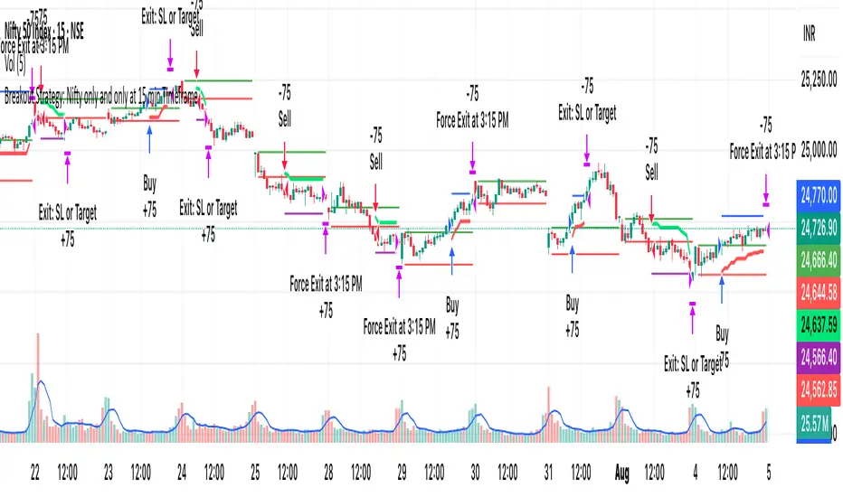
DeltaTrace ForecastDeltaTrace Forecast is a forward-looking projection tool that visualizes the probable directional path of price using a multi-timeframe momentum model rooted in volatility-adjusted nonlinear dynamics. Rather than relying on traditional indicators that react to price after the fact, DeltaTrace estimates future price motion by tracing the progression of momentum changes across expanding timeframes—then scaling those deltas using adaptive volatility to forecast a plausible path forward.
At its core, DeltaTrace constructs a momentum vector from a series of smoothed z-scores derived from increasing multiples of the current chart's timeframe. These z-scores are normalized using a hyperbolic tangent function (tanh), which compresses extreme values and emphasizes meaningful deviations without being overly sensitive to outliers. This nonlinear normalization ensures that explosive moves are weighted with less distortion, while still preserving the shape and direction of the underlying trend.
Once the z-scores are calculated for a range of 12 timeframes (from 1× the current timeframe up to 12×), the indicator computes the first difference between each adjacent pair. These differences—or deltas—represent the change in momentum from one timeframe to the next. In this structure, a strong positive delta implies momentum is strengthening as we look into higher timeframes, while a negative delta reflects waning or reversing strength.
However, not all deltas are treated equally. To make the projection adaptive to market volatility and temporally meaningful, each delta is scaled by the square root of its corresponding timeframe multiple, weighted by the ATR (Average True Range) of the base timeframe. This square-root volatility scaling mirrors the behavior of Brownian motion and reflects the natural geometric diffusion of price over time. By applying this scaling, the model tempers its forecast according to recent volatility while maintaining proportional distance over longer time horizons.
The result is a chain of projected price steps—11 in total—starting from the current closing price. These steps are cumulative, meaning each one builds upon the previous, forming a continuously adjusted polyline that represents the most recent forecast path of price. Each point in the forecast line is directional: if the next projected point is above the last, the segment is colored green (upward momentum); if below, it is colored red (downward momentum). This color coding gives immediate visual feedback on the nature of the projected path and allows for intuitive at-a-glance interpretation.
What makes DeltaTrace unique is its combination of ideas from signal processing, time-series momentum analysis, and volatility theory. Instead of relying on static support/resistance levels or lagging moving averages, it dynamically adapts to both momentum curvature and volatility structure. This allows it to be used not just for trend confirmation, but also for top-down bias fading, reversal anticipation, and path-following strategies.
Traders can use DeltaTrace in a variety of ways depending on their style:
For trend traders, a consistent upward or downward curve in the forecast suggests directional continuation and can be used for position sizing or confirmation of bias.
For mean-reversion traders, exaggerated divergence between the current price and the first few forecast points may indicate temporary exhaustion or overextension.
For scalpers or intraday traders, the short-term bend or flattening of the initial segments can reveal early signs of weakening momentum or build-up before breakout.
For swing traders, the full shape of the polyline gives an evolving map of market rhythm across time compression, allowing for context-aware decision-making.
It’s important to understand that this is a path projection tool, not a precise price target predictor. The forecast does not attempt to predict exact price levels at exact bars, but rather illustrates how the market might evolve if the current multi-timeframe momentum structure persists. Like all models, it should be interpreted probabilistically and used in conjunction with other confirmation signals, risk management tools, or strategy frameworks.
Inputs allow customization of the z-score calculation length and ATR window to tune the sensitivity of the model. The color scheme for up/down forecast segments can also be adjusted for personal preference. Additionally, users can toggle the polyline forecast on or off, which may be useful for pairing this indicator with others in a crowded chart layout.
Because the forecast path is calculated only on the last bar, it does not repaint or shift once the candle closes—preserving historical accuracy for visual inspection and backtesting reference. However, it is also sensitive to changes in volatility and momentum structure, meaning it updates each bar as conditions evolve, making it most effective in real-time decision support.
DeltaTrace Forecast is particularly well-suited for traders who want a deeper understanding of hidden momentum shifts across timeframes without relying on traditional trend-following tools. It reveals the shape of future possibility based on present dynamics, offering a compact yet powerful visualization of directional bias, transition risk, and path strength.
To maximize its utility, consider pairing DeltaTrace with volume profiles, order flow tools, higher timeframe zones, or market structure indicators. Used in context, it becomes a powerful companion to both systematic and discretionary trading styles—especially for those who appreciate a blend of mathematics and intuition in their market analysis.
This indicator is not based on magic or black-box logic; every component—from the z-score standardization to the volatility-adjusted deltas—is fully transparent and grounded in simple, interpretable mechanics. If you're looking for a reliable way to visualize multi-timeframe bias and momentum diffusion, DeltaTrace provides a unique lens through which to interpret future potential in an ever-shifting market landscape.

Bullish/Bearish Trend Indicator [MTF + Alerts] by Dow theory Summary of Logic:
✅ Bullish Trend:
Setup Bar: High > Previous High AND Low ≥ Previous Low
Confirmation Bar: High > Highest High of last 3 candles, Low ≥ Setup Bar Low
Trend Continues Until: Latest candle breaks 2nd last candle’s low → then trend becomes Bearish
🔻 Bearish Trend:
Setup Bar: Low < Previous Low AND High ≤ Previous High
Confirmation Bar: Low < Lowest Low of last 3 candles, High ≤ Setup Bar High
Trend Continues Until: Latest candle breaks 2nd last candle’s high → then trend becomes Bullish