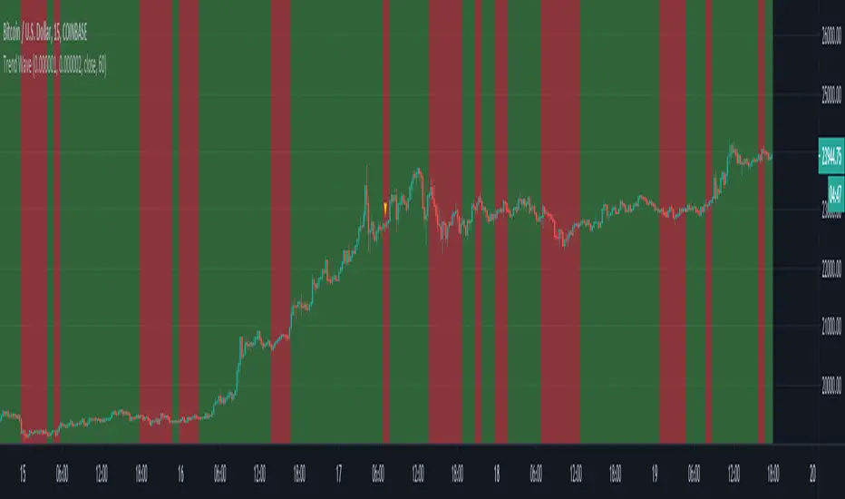
Trend WaveThis indicator is used to filter the trend of stock.
2 period moving average is used to filter the unstable market.
Retracement only max 3 days,to avoid big retrace cause profit burn.
Background color is based on candle color.
Green Candle = Bull Momentum
Yellow Candle = Possible Retrace / Bear Momentum ( to avoid miss the bull wave )
Red Candle = Bear Momentum
❗ = Danger signal - based on volume,candlestick,support
Have a look to the wick to determine the momentum power of bull/bear
Strategy To Trade:
Long when candle turn RED to GREEN
Long when retrace end and BULL momentum appear
Short when candle turn GREEN/YELLOW to RED
Wait for Red Candle to Exit if your cost is low
Not suggest to catch high for day changes% > 15
**PLEASE TRADE USING SEVERAL INDICATOR (NOT ONLY ONE)!!!
Kindly Comment Below For your opinion to this indicator.
This is permanently share to public.
"wave" için komut dosyalarını ara

MTP Wave Price TargetsThe MTP Wave Price Targets script allows you to project “in advance” WPT (Wave Price Target) zones on your chart, these anticipate where the next Elliott Wave swing is likely to end. WPT zones are calculated using clusters of Fibonacci Price levels that are specific to the Wave in question.
This is designed to be used with the users own “manual” Elliot Wave count. The user can use the MTP Pivots (that are included in the MTP Analysis Script) as a guide to see the swings to choose on the Chart. The user has several options (Pivot Number, Last Pivot, Pivots Back or Bar Number) on how to choose the Pivot to display the WPT Targets from.
There is a risk in Trading and Investing. Losses can and will unfold.
The script is available as an “invite-only” script, as part of the MTPredictor suite of tools on Trading View.
To obtain access, please go to the web page in our signature that appears below.

X Wave DetectorThis indicator is designed mainly for day traders who want to use Supply and Demand, but it is good for swing traders too.
X Wave Detector indicator script detects Short Term supply and demand zones. These zones do offer great insight into the structure of any market. If you understand and know how to trade with support and resistance zones, then you might find supply and demand zones very similar.
A list of all the features is provided below.
1. Customize Basing Color
2. Strength of the zone.
3. Number of candles in basing from 1 to 4
4. Color customization for Supply Demand Zone Labels
5. Hide Zone Labels
6. Hide Supply and Demand candles
This indicator/script focuses on strong volume moves to the upside and downside. When price makes a decent move with volume, the indicator will create a supply or demand zone (the candlestick is painted).
How to trade with it:
1. Focus on a price level (zone)
It’s difficult to analyze the market without key levels. If you look for turning points at every key level, you will only find confusion.
How do you know which price level to focus on? Which price levels are potential market turning points?
2. When the market tests a potential demand area, look out for:
Bullish price pattern
Clear trend
Increased volume
Congestion
When the market tests a potential supply area, look out for:
Bearish price pattern
Clear trend
Increased volume
Congestion
Happy Trading and Stay Awesome!
Use it at your own risk. I cannot be held liable for any damages financial or otherwise, directly or indirectly related to using this script.

[blackcat] L2 Ehlers Sine Wave IndicatorLevel: 2
Background
John F. Ehlers introuced Sine Wave Indicator in his "Rocket Science for Traders" chapter 9.
Function
blackcat L2 Ehlers Sine Wave Indicator compared to conventional oscillators such as the Stochastic or Relative Strength Indicator (RSI), the Sinewave Indicator has two major advantages. These are
1. The Sinewave Indicator anticipates the Cycle Mode turning point rather than waiting for confirmation.
2. The phase does not advance when the market is in a Trend Mode. Therefore, the Sinewave Indicator tends to not give false whipsaw signals when the market is in a Trend Mode.
An additional advantage is that the anticipation signal is obtained strictly by mathematically advancing the phase. Momentum is not employed. Therefore, the Sinewave Indicator signals are no more noisy than the original signal.
Key Signal
Smooth --> 4 bar WMA w/ 1 bar lag
Detrender --> The amplitude response of a minimum-length HT can be improved by adjusting the filter coefficients by
trial and error. HT does not allow DC component at zero frequency for transformation. So, Detrender is used to remove DC component/ trend component.
Q1 --> Quadrature phase signal
I1 --> In-phase signal
Period --> Dominant Cycle in bars
SmoothPeriod --> Period with complex averaging
DCPhase ---> dominant cycle phase for sine wave
Pros and Cons
100% John F. Ehlers definition translation of original work, even variable names are the same. This help readers who would like to use pine to read his book. If you had read his works, then you will be quite familiar with my code style.
Remarks
The 8th script for Blackcat1402 John F. Ehlers Week publication.
Readme
In real life, I am a prolific inventor. I have successfully applied for more than 60 international and regional patents in the past 12 years. But in the past two years or so, I have tried to transfer my creativity to the development of trading strategies. Tradingview is the ideal platform for me. I am selecting and contributing some of the hundreds of scripts to publish in Tradingview community. Welcome everyone to interact with me to discuss these interesting pine scripts.
The scripts posted are categorized into 5 levels according to my efforts or manhours put into these works.
Level 1 : interesting script snippets or distinctive improvement from classic indicators or strategy. Level 1 scripts can usually appear in more complex indicators as a function module or element.
Level 2 : composite indicator/strategy. By selecting or combining several independent or dependent functions or sub indicators in proper way, the composite script exhibits a resonance phenomenon which can filter out noise or fake trading signal to enhance trading confidence level.
Level 3 : comprehensive indicator/strategy. They are simple trading systems based on my strategies. They are commonly containing several or all of entry signal, close signal, stop loss, take profit, re-entry, risk management, and position sizing techniques. Even some interesting fundamental and mass psychological aspects are incorporated.
Level 4 : script snippets or functions that do not disclose source code. Interesting element that can reveal market laws and work as raw material for indicators and strategies. If you find Level 1~2 scripts are helpful, Level 4 is a private version that took me far more efforts to develop.
Level 5 : indicator/strategy that do not disclose source code. private version of Level 3 script with my accumulated script processing skills or a large number of custom functions. I had a private function library built in past two years. Level 5 scripts use many of them to achieve private trading strategy.
ATLAS Wave RiderATLAS Wave Rider
Intended Trading Style Use
Scalping
Intended time frame use
10-min and under, ideal on 3-min chart and 5-minute chart.
Funtion
The base calculation of the candlestick chart uses the philosophy of equilibrium in Japanese technical analysis, the code reflects this by utilizing the Japanese moving average of Heiken-Ashi.
Trends are checked against an average of two time periods. They are further filtered according to the open of the unseen Heiken-Ashi and where that open occurs against the two averages. Finally, moves above and below a mean are filtered against a measured parabolic average.
Entries
Buy/Long entries occur when sufficient criteria are met to consider taking a buy/long.
Sell/Short entries occur when sufficient criteria are met to consider taking a sell/short.
Possible exits identify probable zones of safely exiting to protect profit or abandon a losing position.
This indicator is meant to be used on time frames below 10-minutes and it is intended to be used with an active 'eyes on the chart' approach.
Practice effective and efficient risk management.

[A618]Improved Wave channel 3D The Script is an Amalgamation of Two prominent Scripts in One
1. Ehlers 2 Pole ButterWorth Filter
2. Wave Channel 3D
Intuitively,
Buy when Candles are above all the filter Lines
Sell when Candles are below the Filter Lines
CREDITS

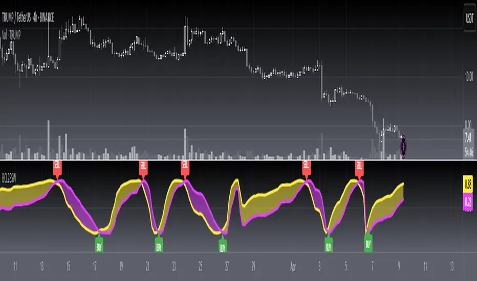
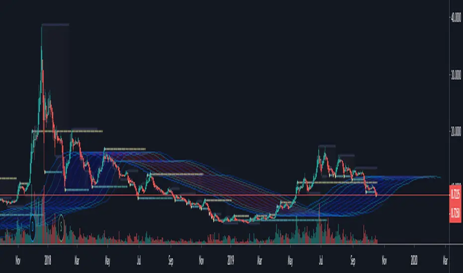
KINSKI Laguerre Filter WaveThe "Laguerre Filter Wave" Indicator usually shows market cycles and is a perfect fit for swing traders who trade with market fluctuations. Upward-trends are shown as green lines and optional bands. Downward trends are represented by the color red. Each of the 18 available lines can be adjusted to your own preferences via a gamma factor.
You also have the following display options:
- "Up/Down Movements: On/Off" - Shows ascending and descending of lines
- "Bands: On/Off" - Fills the space between the lines with colors to indicate up or down trends
- "Bands: Transparency" - sets the transparency of the fill color
- "MA Line: Size" - sets the width of the lines
- "MA Line: Transparency" - sets the transparency of the lines

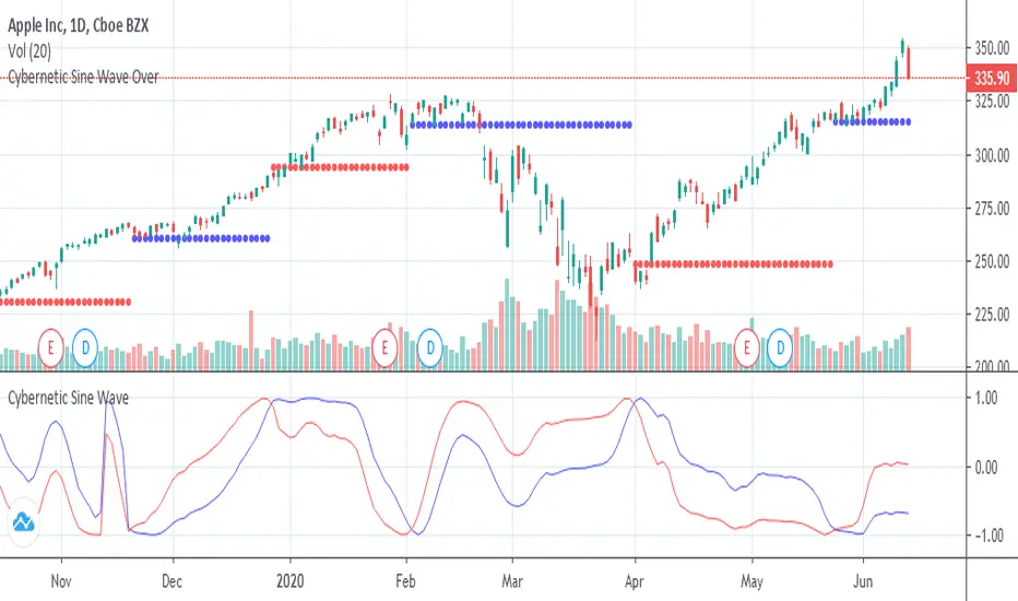
Cybernetic Sine Wave OverOverlay on chart of the support and resistance lines of the "Cybernetic Sine Wave"

Cybernetic Sine WaveThis is John F. Ehlers "Sine Wave Indicator" on the book "Cybernetic Analysis for Stocks and Futures".
When red crosses under blue there is a resistance and the price should fall and when red crosses over blue there is a support and the price should rise, but, the market is always right,
if instead of turning down on the resistance it surpasses it there is a trend up, if instead of turning up on the the support it falls through it there is a trend down.
[HWVZ] Hiubris WeisVolume ZigZagThis script follows the Zig Zag pattern of price movement, based on the Weis Wave Volume indicator.
The Weis Wave Volume shows the cumulative volume from the lowest point of the price swing to the highest point (or vice versa)
The user has the option to change the Trend Detection Length of the indicator to adjust the swings frequency (from say 5 to any value above or below)
The user has the option to display Support & Resistance lines based on those turning points
The user has the option to display Info Labels for each swing
The user has the option to change the Weis Wave Volume Timeframe
*This is a Tradingview interpretation of the Weis Wave Plugin

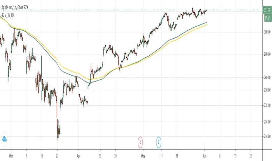
4C Vegas Wave Tunnel EMA(144,169) - RKExtended from 4C Vegas Wave Tunnel EMA(144,169) , credit to FourC
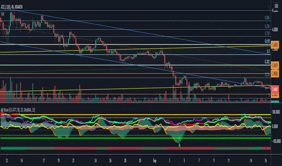
AIMS Wave TVUsing the Logic of the 10 Seconds Elliott Wave
You can Count Elliott Wave on the Histogram of this indicator instead of Price.
This is simpler and more accurate (subjectivity)
Please follow the link below to download FREE EBook which explains how to use this super duper indicator.

Trend WaveHello Traders!
You know, I can sill remember the first time I started tinkering with Pinescript. As I had no prior programming experience, I learned by experimenting with other open-source scripts on TradingViews Marketplace. Tearing apart and combining interesting scripts to see what the output would be. @ChrisMoody was a huge source of inspiration for learning, and I wanted to thank him, as well as @TheLark for the concept behind this script.
The Trend Wave is based on @ChrisMoody's PPO-PercentileRank-Mkt-Tops-Bottoms , which also happens to be based on @TheLark's TheLark-Laguerre-PPO/ .
Within my experimentation, I found that if I isolate the ppoT & ppoB variables and plot them calculated from extremely small decimals, you can get an extremely fast reacting, mirroring trend detector.
Within the script, you have the ability to plot the background colors based on trend to make it easier to see where crossovers occured, as well as a Mirror Input to view the mirrored version of the script.
-@DayTradingOil
Surfing Wave [ChuckBanger]An interesting little script... It utilize Moving Averages with a set multiplier and an offset to locate strong trends and possible future support - resistance. I also include a Donchian wave channel.
The interesting thing with Donchian part is it lines up pretty well with fibonacci retracement
Swing Wave Finder by 2tmHello Everyone.
This is to find Swing Wave's Higher Point and Lower Point.
There are similar scripts but this is pretty different with them.
It is quite helpful when you use with My other script 'Orderblocks'
Thank you and have a nice day.

W5T Bar number for Elliott Wave IsolationSpecial Bar counting tool to allow Isolation of Elliott Wave wave count. Watch the Video Tour >>HERE<<< of this full and comprehensive Elliott Wave Indicator Suite.

W5T Elliott Wave OscillatorSpecial Elliott Wave Oscillator which is part of the W5T Elliott Wave Indicator suite. Watch the quick Video tour >>>HERE<<< and find out about this incredible and complete Elliott Wave Indicator Suite

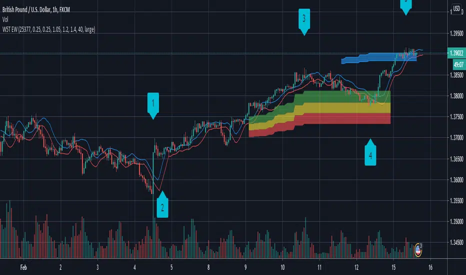
W5T Elliott Wave Indicator SuiteThe Elliott Wave Indicator Suite brings order and reason to the world of Swing Trading, Intraday Trading and Day Trading. It greatly illuminates the path through the forest of chaotic markets versus getting lost among all the trees. Perfect for Stocks, Forex, Futures, Commodities, Indexes and even Crypto Currency markets. Watch the Video Tour and find out More >>>HERE<<<
Includes:
Elliott Wave Indicator
High Probability Pull Back Zones
Elliott Wave isolation
Automated Target Zones
False Breakout Stochastic
Automated Elliott Wave Count
Special 5/35 Pull Back Oscillator
6/4 MA High & Low for Trade Entry & Management
Training Bootcamp
Free Monthly Live Support Webinars
Weis Wave Volume (Pinescript 4)Port of LazyBear's Weis Wave Volume indicator to pinescript v4 from v2.

Weiss Wave Open Interest BarsFirstly :
LazyBear ' s "Weiss Wave " codes are used for open interests.
Original Weiss Wave Volume :
Let's start :
Open Interest vs. Volume: An Overview
Volume and open interest are two key measurements that describe the liquidity and activity of contracts In the options and futures markets. However, their meanings and applications are different. Volume refers to the number of contracts traded in a given period, while open interest denotes the number of active contracts.
Volume
Trading volume measures the number of options or futures contracts being exchanged between buyers and sellers, identifying the level of activity for that particular contract. For every buyer, there is a seller, and the transaction itself counts toward the daily volume.
Open Interest
Open interest indicates the number of options or futures contracts that are held by traders and investors in active positions. These positions have not been closed out, expired, or exercised. Open interest decreases when holders and writers of options (or buyers and sellers of futures) close out their positions. To close out positions, they must take offsetting positions or exercise their options. Open interest increases once again when investors and traders open new long positions or writers/sellers take on new short positions. Open interest also increases when new options or futures contracts are created.
Options or futures contract trading volume can only increase while open interest can either increase or decrease. While trading volume indicates the number of contracts that have been bought or sold, open interest identifies the number of contracts that are currently held.
Reference : www.investopedia.com
*** Worked to define all futures . You can look them in codes (between line : 13 to line 94 )
** CAUTION 1 : Since each instrument in the list has its own unique contract data, you must first enter its name to display it. I recommend you to select OANDA from the markets. Finally, when the COT reports are issued, it may repaints. However, this repaint is usually close to closing or after close .(When COT reports are so sharp ) So use this script only 1W ( 1 week ) or 1 M ( 1 month ) timeframe.
** CAUTION 2 : This data is taken to Tradingview with the help of Quandl. This is a tremendous possibility, but the system will not work if there is a malfunction.
Best regards.