DB Change Forecast ProDB Change Forecast Pro
What does the indicator do?
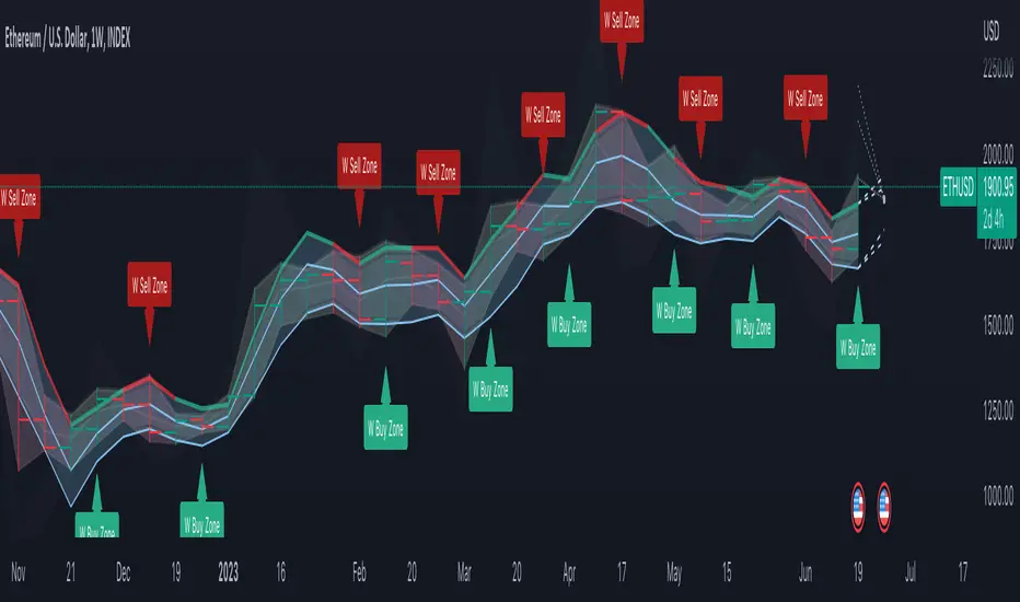
The DB Change Forecast Pro is a unique indicator that uses price change on HLC3 to detect buy and sell periods along with plotting a linear regression price channel with oversold and undersold zones. It also has a linear regression change forecast mode to optionally project market direction.
Change is calculated by taking a two-bar change of HLC3 and dividing that by the price or, optionally, a fixed divisor.
A fast-moving change cloud is then calculated and displayed as the "regular version" plot (shown in light gray). When the cloud bottom is above low, a buy zone is detected. When the cloud top is below the high, a sell zone is detected.
The linear regression price channel is calculated similarly but using a much slower change rate. The linear regression price channel shows reasonable high, low and HLC3 ranges. At the bar's opening, the channel will be more compact and come fairly accurate about 1/4 into the bar timeframe.
The change forecasted price is projected on the right side of the current bar to indicate the current timeframe direction. Please note this forecasting feature is shown in orange when it's early in the timeframe and gray when the timeframe is more likely to produce an accurate direction forecast for the upcoming bar.
You can use these projected dashed lines to see possible market movements for the Current bar and possible market direction for the next bar. Kindly note these projects change; they should be used to understand possible extreme highs/lows for the current bar or market direction.
The indicator includes an optional change forecast projection feature hidden by default. It will project the market forecast channel with an offset of 1. The forecast is defaulted to an offset of 1 to show market direction. However, you can modify to zero the offset to show the current bar forecast and forecast history.
How should this indicator be used?
First, very important,
1. Settings > Set Symbol to Desired
2. Settings > Set High Timeframe to "Chart"
3. Settings > Ensure "Use price as divisor" is checked.
It's recommended to use this indicator in higher timeframes. Buy and sell signals are displayed in real-time. However, waiting until 1/4 to 1/2 into the current bar is recommended before taking action, and change can happen.
The buy/sell signals (zones) provide recommendations on playing a long vs. a short. When in a buy sone, only play longs. When in a sell zone, only play shorts.
Then use the linear regression price channel oversold and undersold zones to optionally open and close positions within the buy/sell zones.
For example, consider opening a long in a buy zone when the linear regression price channel shows undersold. Then consider closing the long when the price moves into the linear regression oversold or higher. Then repeat as long as it's in the buy zone. Then vice versa for sell zones and shorting.
At basic design, buy in the buy zone, sell or short in the sell zone. If you are up for higher trading frequencies, use the linear regression price channel as described in the example above.
Please note, as, with all indicators, you may need to adjust to fit the indicator to your symbol and desired timeframe.
This is only an example of use. Please use this indicator as your own risk and after doing your due diligence.
Does the indicator include any alerts?
Yes,
"DB CFHLC3: Signal BUY" - Is triggered when a buy signal is fired.
"DB CFHLC3: Signal SELL" - Is triggered when a sell signal is fired.
"DB CFHLC3: Zone BUY" - Is triggered when a buy zone is detected.
"DB CFHLC3: Zeon SELL" - Is triggered when a sell zone is detected.
"DB CFHLC3: Oversold SELL" - Is triggered when the price exceeds the oversold level.
"DB CFHLC3: Undersold BUY" - Is triggered when the price goes below the undersold level.
Any other tips?
Once you have configured the indicator for your symbol and chart timeframe. Meaning the plots are displayed over the price. Check out larger timeframes such as W, 2W, 3W, 4W, M, and 4M. It works wonderfully for showing market lows and highs for long-term investing too!
Another, tip is to combine it with your favorite indicator, such as TTM Squeeze or MACD for confirmation purposes. You may be surprised how fast the indicator shows market direction changes on higher timeframes.
You can just as easily use a high timeframe such as D, 2D, or 3D for day trading due to how the linear price channel works.
Why am I not selling this indicator?
I would like to bless the TradingView community, and I enjoy publishing custom indicators.
If you enjoy this indicator, please consider leaving a thumbs up or a comment for others to know about your experience or recommendations.
Enjoy!
Regression
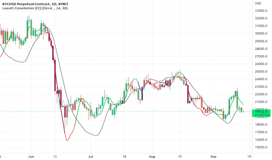
Leavitt Convolution [CC]The Leavitt Convolution indicator was created by Jay Leavitt (Stocks and Commodities Oct 2019, page 11), who is most well known for creating the Volume-Weighted Average Price indicator. This indicator is very similar to my Leavitt Projection script and I forgot to mention that both of these indicators are actually predictive moving averages. The Leavitt Convolution indicator doubles down on this idea by creating a prediction of the Leavitt Projection which is another prediction for the next bar. Obviously this means that it isn't always correct in its predictions but it does a very good job at predicting big trend changes before they happen. The recommended strategy for how to trade with these indicators is to plot a fast version and a slow version and go long when the fast version crosses over the slow version or to go short when the fast version crosses under the slow version. I have color coded the lines to turn light green for a normal buy signal or dark green for a strong buy signal and light red for a normal sell signal, and dark red for a strong sell signal.
This is another indicator in a series that I'm publishing to fulfill a special request from @ashok1961 so let me know if you ever have any special requests for me.
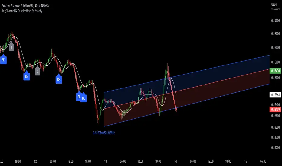
Regression Channel, Candles and Candlestick Patterns by MontyRegression Candles by ugurvu
Regression Channel by Tradingview
All Candlestick Patterns By Tradingview
This script was combined for a friend of mine who needed this.
This Script has regression candles by ugurvu, Regression channel and Candlestick patterns by tradingview.
The intention was to fuse these together so more information can be processed on the cost of a single indicator.
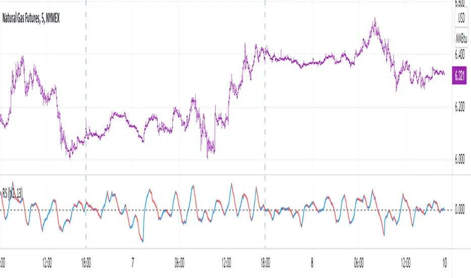
RSI + MA, LinReg, ZZ (HH HL LH LL), Div, Ichi, MACD and TSI HistRelative Strength Index with Moving Average, Linear Regression, Zig Zag (Highs and Lows), Divergence, Ichimoku Cloud, Moving Average Convergence Divergence and True Strength Index Histogram
This script is based on zdmre's RSI script, I revamped a lot of things and added a few indicators from ParkF's RSI script.
Disable Labels in the Style tab and the histogram if you don't enlarge the indicator and it seems too small.
Look to buy in the oversold area and bounce of the support of the linear regression.
Look to sell in the overbought area and bounce of the resistance of the linear regression.
Look for retracement to the moving average or horizontal lines, and divergences for potential reversal.
RSI
The Relative Strength Index (RSI) is a well versed momentum based oscillator which is used to measure the speed (velocity) as well as the change (magnitude) of directional price movements.
Moving Average
Moving Average (MA) is a good way to gauge momentum as well as to confirm trends, and define areas of support and resistance.
Linear Regression
The Linear Regression indicator visualizes the general price trend of a specific part of the chart based on the Linear Regression calculation.
Zig Zag (Highs and Lows)
The Zig Zag indicator is used to identify price trends, and in doing so plots points on the chart to mark whenever prices reverse by a larger percentage point than a predetermined variable or marker.
Divergence
The divergence indicator warns traders and technical analysts of changes in a price trend, oftentimes that it is weakening or changing direction.
Ichimoku Cloud
The Ichimoku Cloud is a package of multiple technical indicators that signal support, resistance, market trend, and market momentum.
MACD and TSI Histogram
MACD can be used to identify aspects of a security's overall trend.
The True Strength Index indicator is a momentum oscillator designed to detect, confirm or visualize the strength of a trend.

R2-Adaptive RegressionOVERVIEW
This is an implementation of alexgrover's R2-Adaptive Regression optimized for the latest version of TradingView.
Full details on the indicator are on alexgrover's page here:

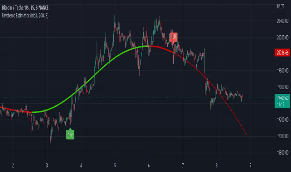
Faytterro EstimatorWhat is Faytterro Estimator?
This indicator is an advanced moving average.
What it does?
This indicator is both a moving average and at the same time, it predicts the future values that the price may take based on the values it has taken before.
How it does it?
takes the weighted average of data of the selected length (reducing the weight from the middle to the ends). then draws a parabola through the last three values, creating a predicted line.
How to use it?
it is simple to use. You can use it both as a regression to review past prices, and to predict the future value of a price. uptrends are in green and downtrends are in red. color change indicates a possible trend change.
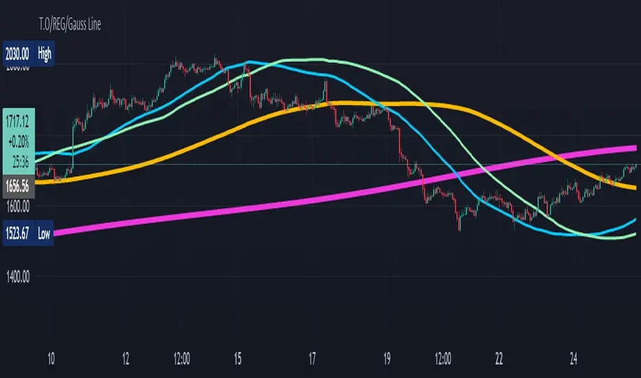
T.O/REG/Gauss LineHi Dear Traders/Dealers!
I present you here 3 lines that I developed myself base on statistical issues.
+Reg. Line
+Gauss Line
+T.O Line
-Reg. Line based on linear regression of previous inputs to make an average value.
-Gauss Line based on Gaussian mean value, Standard Deviation and it uses previous inputs to make an average value.
-T.O Line based on Gaussian and RMA methods generate an average value.
Hopefully useful for you!
Best regards and happy trading
Shakib
Polynomial Regression Derivatives [Loxx]Polynomial Regression Derivatives is an indicator that explores the different derivatives of polynomial position. This indicator also includes a signal line. In a later release, alerts with signal markings will be added.
Polynomial Derivatives are as follows
1rst Derivative - Velocity: Velocity is the directional speed of a object in motion as an indication of its rate of change in position as observed from a particular frame of reference and as measured by a particular standard of time (e.g. 60 km/h northbound). Velocity is a fundamental concept in kinematics, the branch of classical mechanics that describes the motion of bodies.
2nd Derivative - Acceleration: In mechanics, acceleration is the rate of change of the velocity of an object with respect to time. Accelerations are vector quantities (in that they have magnitude and direction). The orientation of an object's acceleration is given by the orientation of the net force acting on that object.
3rd Derivative - Jerk: In physics, jerk or jolt is the rate at which an object's acceleration changes with respect to time. It is a vector quantity (having both magnitude and direction). Jerk is most commonly denoted by the symbol j and expressed in m/s3 (SI units) or standard gravities per second (g0/s).
4th Derivative - Snap: Snap, or jounce, is the fourth derivative of the position vector with respect to time, or the rate of change of the jerk with respect to time. Equivalently, it is the second derivative of acceleration or the third derivative of velocity.
5th Derivative - Crackle: The fifth derivative of the position vector with respect to time is sometimes referred to as crackle. It is the rate of change of snap with respect to time.
6nd Derivative - Pop: The sixth derivative of the position vector with respect to time is sometimes referred to as pop. It is the rate of change of crackle with respect to time.
Included:
Loxx's Expanded Source Types
Loxx's Moving Averages

Regression Channel Trend DetectionThis is a regression channel that uses ichimoku to determine trend. The sensitivity is customizable. The centerline will change color according to the trend detected by ichimoku, and each line can act as support/resistance. The bands of the channel also change colors according to how far price is getting away from them. If you notice in this example, the lower band is turning orange when the price is getting too far away from it, suggesting that it may have risen too fast and too soon. This is still in testing so feel free to comment with any suggestions or fixes.
Polynomial-Regression-Fitted RSI [Loxx]Polynomial-Regression-Fitted RSI is an RSI indicator that is calculated using Polynomial Regression Analysis. For this one, we're just smoothing the signal this time. And we're using an odd moving average to do so: the Sine Weighted Moving Average. The Sine Weighted Moving Average assigns the most weight at the middle of the data set. It does this by weighting from the first half of a Sine Wave Cycle and the most weighting is given to the data in the middle of that data set. The Sine WMA closely resembles the TMA (Triangular Moving Average). So we're trying to tease out some cycle information here as well, however, you can change this MA to whatever soothing method you wish. I may come back to this one and remove the point modifier and then add preliminary smoothing, but for now, just the signal gets the smoothing treatment.
What is Polynomial Regression?
In statistics, polynomial regression is a form of regression analysis in which the relationship between the independent variable x and the dependent variable y is modeled as an nth degree polynomial in x. Polynomial regression fits a nonlinear relationship between the value of x and the corresponding conditional mean of y, denoted E(y |x). Although polynomial regression fits a nonlinear model to the data, as a statistical estimation problem it is linear, in the sense that the regression function E(y | x) is linear in the unknown parameters that are estimated from the data. For this reason, polynomial regression is considered to be a special case of multiple linear regression .
Included
Alerts
Signals
Bar coloring
Loxx's Expanded Source Types
Loxx's Moving Averages
Other indicators in this series using Polynomial Regression Analysis.
Poly Cycle
PA-Adaptive Polynomial Regression Fitted Moving Average
Polynomial-Regression-Fitted Oscillator
Polynomial-Regression-Fitted Oscillator [Loxx]Polynomial-Regression-Fitted Oscillator is an oscillator that is calculated using Polynomial Regression Analysis. This is an extremely accurate and processor intensive oscillator.
What is Polynomial Regression?
In statistics, polynomial regression is a form of regression analysis in which the relationship between the independent variable x and the dependent variable y is modeled as an nth degree polynomial in x. Polynomial regression fits a nonlinear relationship between the value of x and the corresponding conditional mean of y, denoted E(y |x). Although polynomial regression fits a nonlinear model to the data, as a statistical estimation problem it is linear, in the sense that the regression function E(y | x) is linear in the unknown parameters that are estimated from the data. For this reason, polynomial regression is considered to be a special case of multiple linear regression .
Things to know
You can select from 33 source types
The source is smoothed before being injected into the Polynomial fitting algorithm, there are 35+ moving averages to choose from for smoothing
This indicator is very processor heavy. so it will take some time load on the chart. Ideally the period input should allow for values from 1 to 200 or more, but due to processing restraints on Trading View, the max value is 80.
Included
Alerts
Signals
Bar coloring
Other indicators in this series using Polynomial Regression Analysis.
Poly Cycle
PA-Adaptive Polynomial Regression Fitted Moving Average

TF Segmented Polynomial Regression [LuxAlgo]This indicator displays polynomial regression channels fitted using data within a user selected time interval.
The model is fitted using the same method described in our previous script:
Settings
Degree: Degree of the fitted polynomial
Width: Multiplicative factor of the model RMSE. Controls the width of the polynomial regression's channels
Timeframe: Fits the polynomial regression using data within the selected timeframe interval
Show fit for new bars: If selected, will fit the regression model for newly generated bars, else the previous fitted value is displayed.
Src: Input source
Usage
Segmented (or piecewise) models yield multiple fits by first partitioning the data into multiple intervals from specific partitioning conditions. In this script this partitioning condition is for a user selected timeframe to change.
Segmented models can be particularly pertinent for market prices, which often describes a series of local trends.
Segmented polynomial regressions can describe the nature of underlying trends in the price from their fit, such as if an underlying trend is more linear (trending) or constant (ranging), and if a trend is monotonic.
The above chart shows a monthly partitioning on SPX 15m, using a polynomial regression of degree 3. Channel extremities allows highlighting local tops/bottoms.
For real time applications users can choose to fit a current model to incoming price data using the Show fit for new bars settings.
Details
The script does not make use of line.new to display the segmented linear regressions, which allows showing a higher number of historical fits. Each channel extremity as well as the model fit is displayed from the plot function, as such user can more easily set alerts on them.
It is important to note that achieving this requires accessing future price data, as such this script is subject to lookahead bias, historical results differ from the results one could have obtained in real-time.

Regression Channel Alternative MTF█ OVERVIEW
This indicator displays 3 timeframes of parallel channel using linear regression calculation to assist manual drawing of chart patterns.
This indicator is not true Multi Timeframe (MTF) but considered as Alternative MTF which calculate 100 bars for Primary MTF, can be refer from provided line helper.
The timeframe scenarios are defined based on Position, Swing and Intraday Trader.
█ INSPIRATIONS
These timeframe scenarios are defined based on Harmonic Trading : Volume Three written by Scott M Carney.
By applying channel on each timeframe, MW or ABCD patterns can be easily identified manually.
This can also be applied on other chart patterns.
█ CREDITS
Scott M Carney, Harmonic Trading : Volume Three (Reaction vs. Reversal)
█ TIMEFRAME EXPLAINED
Higher / Distal : The (next) longer or larger comparative timeframe after primary pattern has been identified.
Primary / Clear : Timeframe that possess the clearest pattern structure.
Lower / Proximate : The (next) shorter timeframe after primary pattern has been identified.
Lowest : Check primary timeframe as main reference.
█ EXAMPLE OF USAGE / EXPLAINATION

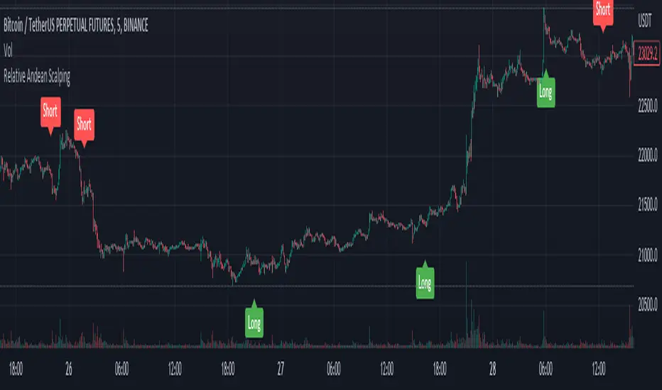
Relative Andean ScalpingThis is an experimental signal providing script for scalper that uses 2 of open source indicators.
First one provides the signals for us called Andean Oscillator by @alexgrover . We use it to create long signals when bull line crosses over signal line while being above the bear line. And reverse is true for shorts where bear line crosses over signal line while being above bull line.
Second one is used for filtering out low volatility areas thanks to great idea by @HeWhoMustNotBeNamed called Relative Bandwidth Filter . We use it to filter out signals and create signals only when the Relative Bandwith Line below middle line.
The default values for both indicators changed a bit, especially used linreg values to create relatively better signals. These can be changed in settings. Please be aware that i did not do extensive testing with this indicator in different market conditions so it should be used with caution.
Linear Regression ChannelsThese channels are generated from the current values of the linear regression channel indicator, the standard deviation is calculated based off of the RSI . This indicator gives an idea of when the linear regression model predicts a change in direction.
You are able to change the length of the linear regression model, as well as the size of the zone. A negative zone size will make the zone stretch away from the center, and a positive zone size will make it stretch towards the centerline.

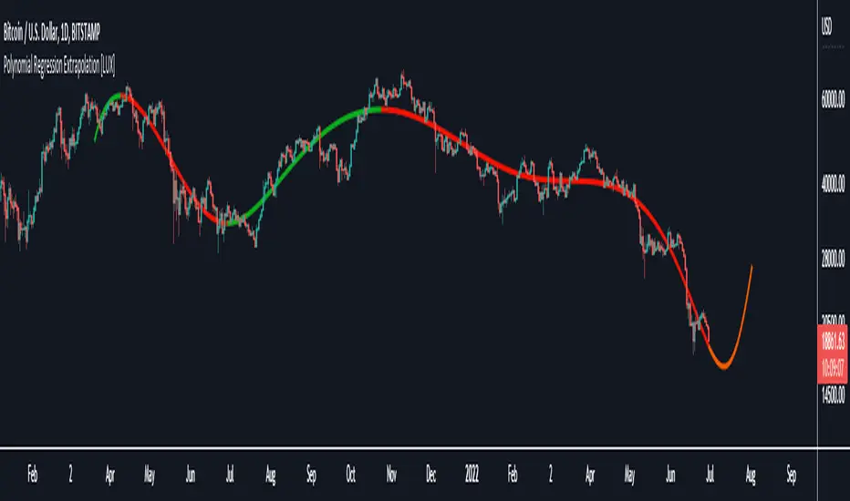
Polynomial Regression Extrapolation [LuxAlgo]This indicator fits a polynomial with a user set degree to the price using least squares and then extrapolates the result.
Settings
Length: Number of most recent price observations used to fit the model.
Extrapolate: Extrapolation horizon
Degree: Degree of the fitted polynomial
Src: Input source
Lock Fit: By default the fit and extrapolated result will readjust to any new price observation, enabling this setting allow the model to ignore new price observations, and extend the extrapolation to the most recent bar.
Usage
Polynomial regression is commonly used when a relationship between two variables can be described by a polynomial.
In technical analysis polynomial regression is commonly used to estimate underlying trends in the price as well as obtaining support/resistances. One common example being the linear regression which can be described as polynomial regression of degree 1.
Using polynomial regression for extrapolation can be considered when we assume that the underlying trend of a certain asset follows polynomial of a certain degree and that this assumption hold true for time t+1...,t+n . This is rarely the case but it can be of interest to certain users performing longer term analysis of assets such as Bitcoin.
The selection of the polynomial degree can be done considering the underlying trend of the observations we are trying to fit. In practice, it is rare to go over a degree of 3, as higher degree would tend to highlight more noisy variations.
Using a polynomial of degree 1 will return a line, and as such can be considered when the underlying trend is linear, but one could improve the fit by using an higher degree.
The chart above fits a polynomial of degree 2, this can be used to model more parabolic observations. We can see in the chart above that this improves the fit.
In the chart above a polynomial of degree 6 is used, we can see how more variations are highlighted. The extrapolation of higher degree polynomials can eventually highlight future turning points due to the nature of the polynomial, however there are no guarantee that these will reflect exact future reversals.
Details
A polynomial regression model y(t) of degree p is described by:
y(t) = β(0) + β(1)x(t) + β(2)x(t)^2 + ... + β(p)x(t)^p
The vector coefficients β are obtained such that the sum of squared error between the observations and y(t) is minimized. This can be achieved through specific iterative algorithms or directly by solving the system of equations:
β(0) + β(1)x(0) + β(2)x(0)^2 + ... + β(p)x(0)^p = y(0)
β(0) + β(1)x(1) + β(2)x(1)^2 + ... + β(p)x(1)^p = y(1)
...
β(0) + β(1)x(t-1) + β(2)x(t-1)^2 + ... + β(p)x(t-1)^p = y(t-1)
Note that solving this system of equations for higher degrees p with high x values can drastically affect the accuracy of the results. One method to circumvent this can be to subtract x by its mean.
Colorful RegressionColorful Regression is a trend indicator. The most important difference of it from other moving averages and regressions is that it can change color according to the momentum it has. so that users can have an idea about the direction, orientation and speed of the graph at the same time. This indicator contains 5 different colors. Black means extreme downtrend, red means downtrend, yellow means sideways trend, green means uptrend, and white means extremely uptrend. I recommend using it on the one hour chart. You can also use it in different time periods by changing the sensitivity settings.

Everything Bitcoin [Kioseff Trading]Hello!
This script retrieves most of the available Bitcoin data published by Quandl; the script utilizes the new request.security_lower_tf() function.
Included statistics,
True price
Volume
Difficulty
My Wallet # Of Users
Average Block Size
api.blockchain size
Median Transaction Confirmation Time
Miners' Revenue
Hash Rate
Cost Per Transaction
Cost % of Transaction Volume
Estimated Transaction Volume USD
Total Output Volume
Number Of Transactions Per Block
# of Unique BTC Addresses
# of BTC Transactions Excluding Popular Addresses
Total Number of Transactions
Daily # of Transactions
Total Transaction Fees USD
Market Cap
Total BTC
Retrieved data can be plotted as line graphs; however, the data is initially split between two tables.
The image above shows how the requested Bitcoin data is displayed.
However, in the user inputs tab, you can modify how the data is displayed.
For instance, you can append the data displayed in the floating statistics box to the stagnant statistics box.
The image above exemplifies the instance.
You can hide any and all data via the user inputs tab.
In addition to data publishing, the script retrieves lower timeframe price/volume/indicator data, to which the values of the requested data are appended to center-right table.
The image above shows the script retrieving one-minute bar data.
Up arrows reflect an increase in the more recent value, relative to the immediately preceding value.
Down arrows reflect a decrease in the more recent value relative to the immediately preceding value.
The ascending minute column reflects the number of minutes/hours (ago) the displayed value occurred.
For instance, 15 minutes means the displayed value occurred 15 minutes prior to the current time (value).
Volume, price, and indicator data can be retrieved on lower timeframe charts ranging from 1 minute to 1440 minutes.
The image above shows retrieved 5-minute volume data.
Several built-in indicators are included, to which lower timeframe values can be retrieved.
The image above shows LTF VWAP data. Also distinguished are increases/decreases for sequential values.
The image above shows a dynamic regression channel. The channel terminates and resets each fiscal quarter. Previous channels remain on the chart.
Lastly, you can plot any of the requested data.
The new request.security_lower_tf() function is immensely advantageous - be sure to try it in your scripts!

Infiten's Regressive Trend Channel An experiment using Pinescript's candle plotting feature. This indicator performs a linear regression on the lows, highs, and moving average, and plots them all in the form of a candlestick. If the close is below the prediction, the candlestick is red, if the close is above the regression, the candlestick is green. Effective and aesthetic way to analyze trends.

Relative slopeRelative slope metric
Description:
I was in need to create a simple, naive and elegant metric that was able to tell how strong is the trend in a given rolling window. While abstaining from using more complicated and arguably more precise approaches, I’ve decided to use Linearly Weighted Linear Regression slope for this goal. Outright values are useful, but the problem was that I wasn’t able to use it in comparative analysis, i.e between different assets & different resolutions & different window sizes, because obviously the outputs are scale-variant.
Here is the asset-agnostic, resolution-agnostic and window size agnostic version of the metric.
I made it asset agnostic & resolution agnostic by including spread information to the formula. In our case it's weighted stdev over differenced data (otherwise we contaminate the spread with the trend info). And I made it window size agnostic by adding a non-linear relation of length to the output, so finally it will be aprox in (-1, 1) interval, by taking square root of length, nothing fancy. All these / 2 and * 2 in unexpected places all around the formula help us to return the data to it’s natural scale while keeping the transformations in place.
Peace TV
StrengthA mathematically elegant, native & modern way how to measure velocity/ strength/ momentum. As you can see it looks like MACD, but !suddenly! has N times shorter code (disregard the functions), and only 1 parameter instead of 3. OMG HOW DID HE DO IT?!?
MACD: "Let's take one filter (1 parameter), than another filter (2 parameters), then let's take dem difference, then let's place another filter over the difference (3rd parameter + introduction of a nested calculation), and let's write a whole book about it, make thousands of multi-hours YouTube videos about it, and let's never mention about the amount of uncertainty being introduced by multiple parameters & introduction of the nested calculation."
Strength: "let's get real, let's drop a weighted linear regression & usual linear regression over the data of the same length, take dem slopes, then make the difference over these slopes, all good. And then share it with people w/o putting an ® sign".
Fyi, regressions were introduced centuries ago, maybe decades idk, the point is long time ago, and computational power enough to calculate what I'm saying is slightly more than required for macd.
Rationale.
Linearly weighted linear regression has steeper slope (W) than the usual linear regression slope (S) due to the fact that the recent datapoints got more weight. This alone is enough of a metric to measure velocity. But still I've recalled macd and decided to make smth like it cuz I knew it'll might make you happy. I realized that S can be used instead of smoothing the W, thus eliminating the nested calculation and keeping entropy & info loss in place. And see, what we get is natural, simple, makes sense and brings flex. I also wanna remind you that by applying regression we maximize the info gain by using all the data in the window, instead of taking difference between the first and the last datapoints.
This script is dedicated to my friend Fabien. Man, you were the light in the darkness in that company. You'll get your alien green Lambo if you'll really want it, no doubts on my side bout that.
Good hunting

Weighted Least Squares Moving AverageLinearly Weighted Ordinary Least Squares Moving Regression
aka Weighted Least Squares Moving Average -> WLSMA
^^ called it this way just to for... damn, forgot the word
Totally pwns LSMA for some purposes here's why (just look up):
- 'realistically' the same smoothness;
- less lag;
- less overshoot;
- more or less same computationally intensive.
"Pretty cool, huh?", Bucky Roberts©, thenewboston
Now, would you please (just look down) and see the comparison of impulse & step responses:
Impulse responses
Step responses
Ain't it beautiful?
"Motivation behind the concept & rationale", by gorx1
Many been trippin' applying stats methods that require normally distributed data to time series, hence all these B*ll**** Bands and stuff don't really work as it should, while people blame themselves and buy snake oil seminars bout trading psychology, instead of using proper tools. Price... Neither population nor the samples are neither normally nor log-normally distributed. So we can't use all the stuff if we wanna get better results. I'm not talking bout passing each rolling window to a stat test in order to get the proper descriptor, that's the whole different story.
Instead we can leverage the fact that our data is time-series hence we can apply linear weighting, basically we extract another info component from the data and use it to get better results. Volume, range weighting don't make much sense (saying that based on both common sense and test results). Tick count per bar, that would be nice tho... this is the way to measure "intensity". But we don't have it on TV unfortunately.
Anyways, I'm both unhappy that no1 dropped it before me during all these years so I gotta do it myself, and happy that I can give smth cool to every1
Here is it, for you.
P.S.: the script contains standalone functions to calculate linearly weighted variance, linearly weighted standard deviation, linearly weighted covariance and linearly weighted correlation.
Good hunting
Linear Regression Channel - Auto Volume BasedBased on oryginal TV indicator BUT with a little twist. ;)
I really like the regression channel - but the problem is that the length needs to be always manually adjusted.
In this script I try to solve this issue.
This is modified version on TV indicator - Linear Regression Channel.
The main difference is that now you don't get static length - it is automatically adjuested to the recent price action (determined by highest volume in last 300 bars).
