Keltner Channels Bands (RMA)Keltner Channel Bands
These normally consist of:
Keltner Channel Upper Band = EMA + Multiplier ∗ ATR
Keltner Channel Lower Band = EMA − Multiplier ∗ ATR
However instead of using ATR we are using RMA
This gives us a much smoother take of the KCB
We are also using 2 sets of bands built on 1 Moving average, this is a common set up for mean reversion strategies.
This can often be paired with RSI for lower timeframe divergences
Divergence
This is using the RSI to calculate when price sets new lows/highs whilst the RSI movement is in the opposite direction.
The way this is calculated is slightly different to traditional divergence scripts. instead of looking for pivot highs/lows in the RSI we are logging the RSI value when price makes it pivot highs/lows.
Gradient Bands
The Gradient Colouring on the bands is measuring how long price has been either side of the MA.
As Keltner bands are commonly used as a mean reversion strategy, I thought it would be useful to see how long price has been trending in a certain direction, the stronger the colours get,
the longer price has been trending that direction which could suggest we are looking for a retrace soon.
Alerts
Alerts included let you choose whether you want to receive an alert for the inside, outside or both band touches.
To set up these alerts, simply toggle them on in the settings, then click on the 3 dots next to the indicators name, from there you click 'Add Alert'.
From there you can customise the alert settings but make sure to leave the 2 top boxes which control the alert conditions. They will be default selected onto your correct settings, the rest you may want to change.
Once you create the alert, it will then trigger as soon as price touches your chosen inside/outside band.
Suggestions
Please feel free to offer any suggestions which you think could improve the script
Disclaimer
The default settings/parameters were shared by Jimtalbott, feel free to play about with the and use this code to make your own strategies.
Mean

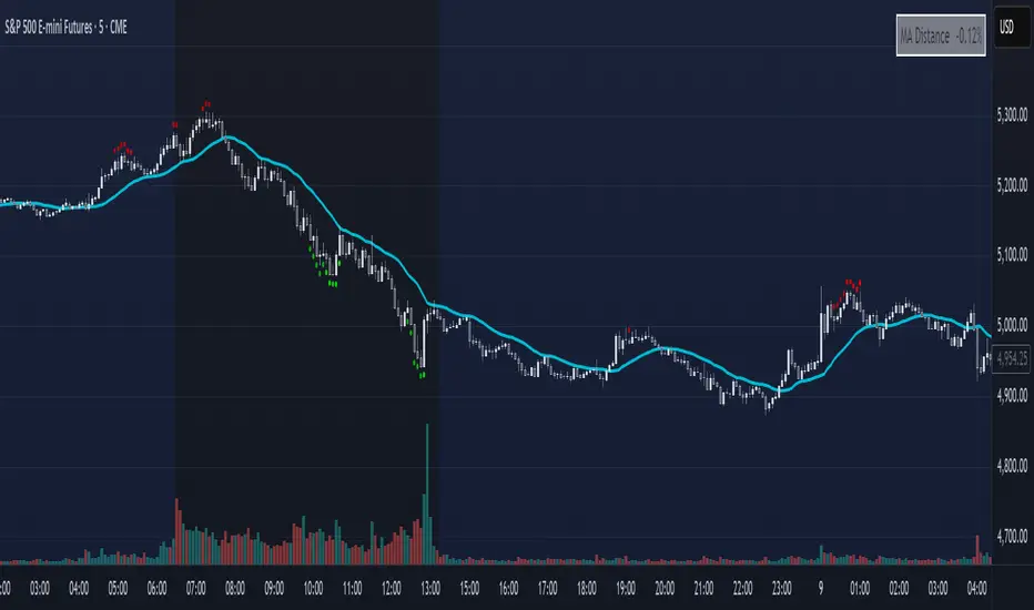
Mean Reversion DotsMarkets tend to mean revert. This indicator plots a moving average from a higher time frame (type of MA and length selectable by the user). It then calculates standard deviations in two dimensions:
- Standard deviation of move of price away from this moving average
- Standard deviations of number of bars spent in this extended range
The indicator plots a table in the upper right corner with the % of distance of price from the moving average. It then plots 'mean reversion dots' once price has been 1 or more standard deviations away from the moving average for one or more standard deviations number of bars. The dots change color, becoming more intense, the longer the move persists. Optionally, the user can display the standard deviations in movement away from the moving average as channels, and the user can also select which levels of moves they want to see. Opting to see only more extreme moves will result in fewer signals, but signals that are more likely to imminently result in mean reversion back to the moving average.
In my opinion, this indicator is more likely to be useful for indices, futures, commodities, and select larger cap names.
Combinations I have found that work well for SPX are plotting the 30min 21ema on a 5min chart and the daily 21ema on an hourly chart.
In many cases, once mean reversion dots for an extreme enough move (level 1.3 or 2.2 and above) begin to appear, a trade may be initiated from a support/resistance level. A safer way to use these signals is to consider them as a 'heads up' that the move is overextended, and then look for a buy/sell signal from another indicator to initiate a position.
Note: I borrowed the code for the higher timeframe MA from the below indicator. I added the ability to select type of MA.
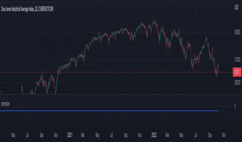
normsinvLibrary "normsinv"
Description:
Returns the inverse of the standard normal cumulative distribution.
The distribution has a mean of zero and a standard deviation of one; i.e.,
normsinv seeks that value z such that a normal distribtuion of mean of zero
and standard deviation one is equal to the input probability.
Reference:
github.com
normsinv(y0)
Returns the inverse of the standard normal cumulative distribution. The distribution has a mean of zero and a standard deviation of one.
Parameters:
y0 : float, probability corresponding to the normal distribution.
Returns: float, z-score
MTFT Last HML wOpen, TheStrat Suite (3of5)Multi Time Frame Tools
Multi Time Frame Tools (MTFT) is a suite of scripts aimed to establish a standard timeframe-based color scheme. This can be utilized to overlay different timeframes calculations/values over a single timeframe. As one example, this would allow to observe the 5-month moving average, 5-week moving average, and 5-day moving average overlaid over each other. This would allow to study a chart, get accustomed to the color scheme and study all these at the same time much easier.
All indicators calculated using the below specific timeframes as input, will always use the color scheme outlined below. This is to get you in habit of recognizing the different timeframes overlaid in top of each other. These can be personalized.
Longer TF analysis.
Yearly - Black
Semi-Annual - Yellow
Quarterly - White
Monthly - Maroon
Weekly - Royal Blue
Daily - Lime
Shorter TF analysis.
4 hour - Fuchsia
1 hour - Orange
30 min - Red
15 min - Brown
10 min - Purple
5 min - Lilac
All color coordination is able to be modified in either the “Inputs” or “Style” section. If you need to make changes, make sure to select “Save as Default” on the bottom right of the settings menu.
Recommended Chart Color Layout
I played around with color coordination a lot. The final product was what worked best for me. I personally use the following chart settings to accent all available TF colors.
-> Click on the settings wheel on your chart. -> Click on “Appearance”.
Background - Solid -> On the top row pick the 6th color from the left.
Vert Grid Lines and Horz Grid Lines -> On the top row pick the 7th color from the left.
You may of course change these and the indicator line colors as you like.
Adding indicator to Chart
-> Open the TradingView “Indicators & Strategies” library, the icon has “ƒx”. -> All premium scripts will be located under “Invite-Only Scripts” -> Click indicator to add to your chart.
MTFT TheStrat Suite (5 Scripts)
Rob Smith is the creator of ‘TheStrat’ trading strategy. For ‘TheStrat’ I have put together a suite of 5 premium scripts that combined will offer people interested in learning ‘TheStrat’ a cleaner learning process. For 2 of the 5 scripts specifically, the MTFT approach of overlaying multiple longer timeframes(TF) over a shorter TF selected as a display cannot be utilized. The other 2 scripts will have full MTFT functionality and they are my personal favorite. I will be providing very basic info to utilize this script; it is up to you to dive deep into learning this strategy. I am not an expert with the tool or a financial advisor. As with all aspects of life, I recommend you research, learn, discern and practice extensively in order to become a master.
1. MTFT Patterns Pro/Noob
2. MTFT Full Time Frame Continuity Table
*3. MTFT Last HML wOpen
4. MTFT Actionable Signal Targets
5. MTFT Reversal Lines
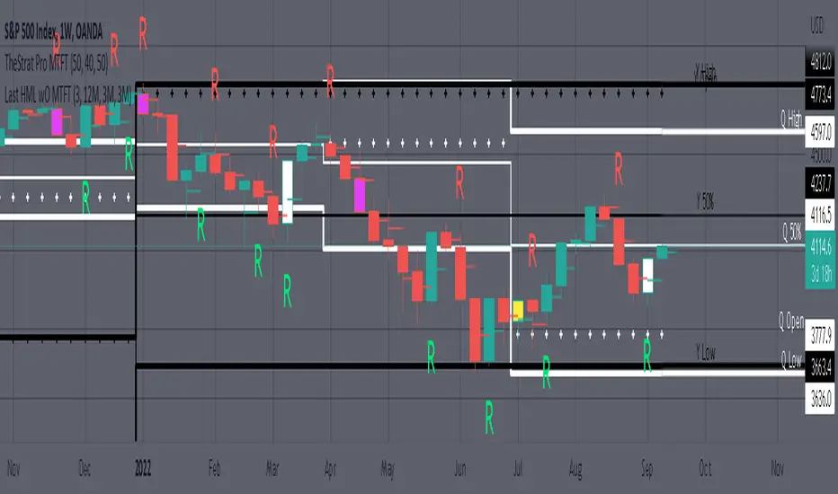
MTFT Last HML wOpen, TheStrat Suite (3of5)
Plots previous High, Mean(50% line), and Low of the previous candlestick and the open for the active TF. This allows you to see how TheStrat Absolute Truths move within the different timeframes. In the image below you see the monthly TF selected. Price on the monthly candlestick has created several reversals up and down.
Now Utilizing this tool, you get to see how priced moved on the daily TF with the previous monthly HML lines plotted(Maroon lines) over the active month so you can see exactly how the absolute truths occur inside each month. Notice the previous High/Low are a thicker width then the Mean, this outlines more clearly which of the lines you are looking at. I’ve included some comments on basic observations.
Now for contrast, below I show you the daily TF selected with the previous quarter HML lines plotted(White lines) over the active quarter.
Script Features includes:
1. Three Timeframes per script instance. Example below shows 3 timeframes in use, Yearly(Black Lines), Quarterly( White Lines), and Monthly (Maroon Lines) on the weekly timeframe candlestick. This is where using a timeframe-based color scheme per individual timeframe will come in very handy. The open of the active timeframe is displayed using the small circles that make a line. The displayed open feature is another way to track full time frame continuity if you are tracking the open of several timeframes. The open of the active timeframe is displayed using the small circles that make a line.
2. 20 different TF to pick from per slot. Timeframes(TF) include: Yearly(Y), Semi-annually(S), Quarterly(Q), Monthly(M), 2-Week(2W), Weekly(W), 3-Day(3D), Daily(D), 12 hour, 8 hour, 6 hour, 4 hour, 3 hour, 2 hour, 1 hour, 30 min, 15 min, 10 min, 5 min. Notice: 2W, 3D, 2D, 12h, 8h, 6h, 3h, and 2h don’t have a supported color scheme as I do not personally use them. They are available to pick from in the timeframe selection and you can set a color for these timeframes under the “Unsupported Color Scheme” section in the settings menu for the script if you would like to use them.
3. Enable/Disable High, Mean, Low or Open on any of the timeframe slots. Custom selection of plots will create clarity in observing timeframe-based analysis. Example below shows the Yearly Open enabled on a Monthly timeframe candlestick selected, along with the 6-month HML lines(This is similar to the quarter, the semi-annual)it shows how the start of the year gave a clear direction several times in the past few years for BTC/USD. A similar analysis can be done across multiple settings. TheStrat Actionable Signals paired with ideas like these can be great setups.
4. Auto-hide timeframes based on specific timeframes selected. For this script, I look for HML lines to have at least 4 total candlesticks within the selected TF. I disable any setting that has 3 or less candlesticks. This applies to all timeframes. This will allow for you to leave several instances of the script in your chart and zoom in and out to see macro/micro levels of a chart. The example below has 2 different instances of the script enabled, first instance (Y, Q, M), and second instance (W, D, 4h). with the Month candlestick selected. Notice how only the Year HML plots are displayed. All other lower timeframes are hidden, this will allow for an easy transition into a lower timeframe analysis.
Same example as above, but now with the Weekly timeframe candlestick selected. Notice that without changing any settings on the scripts the Quarterly (White) and Monthly (Maroon) are now visible.
One more time, this time with the 30m candlestick timeframe selected. Notice that without changing any settings on the scripts the Day(Green) and the 4 hour(Pink) plots appear.
5. Custom Width Selection in script settings per plot type, High, Mean, Low and Open.
IMPORTANT NOTE for TradingView Admin: One of the lessons I would consider most important in attaining clarity regarding trading, is “TheStrat” by Rob Smith. His lesson on “actionable signals” is something that can be applied to any strategy. For this reason, I am including “MTFT TheStrat Patterns Pro” script in all images that will depict confluence for a better trade selection.
Example using TheStrat Pro MTFT with this indicator.
Look for a “TheStrat actionable signal” or a “TheStrat Reversal signal” on a smaller timeframe that has an instance of this indicator on a larger timeframe calculation that is in range of the candlestick that formed your actionable signal. This means that the indicators plot you are observing must be above the low and below the high of the candlestick that is the actionable signal/reversal signal. Image below shows what this would look like with this indicator.
The Image below shows what this would look like with this indicator. The selected timeframe is the Daily, it shows an ‘H’ char below which is an indication of a Hammer Actionable signal and the low from last week is in range showing some potential support. This actionable signal is meant to be played for LONGS. If the high is breached than you would enter a LONG position. For targets you would look at the previous pivots, for this example all targets were hit. This won’t always play out so nice and clean, but given that there is so many stocks and so many signals this is just a thought to improve the quality of the signal as it has extra confluence.
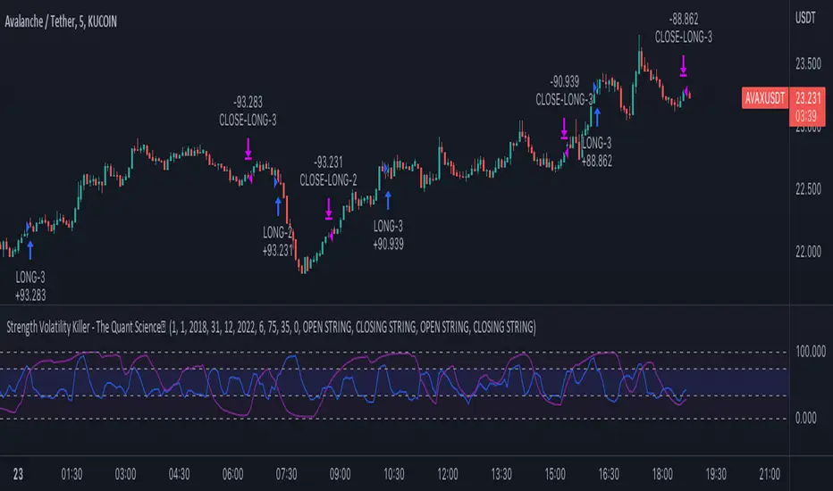
Strength Volatility Killer - The Quant ScienceStrength Volatility Killer - The Quant Science™ is based on a special version of RSI (Relative Strength Index), created with the simple average and standard deviation.
DESCRIPTION
The algorithm analyses the market and opens positions following three different volatility entry conditions. Each entry has a specific and personal exit condition. The user can setting trailing stop loss from user interface.
USER INTERFACE SETTING
Configures the algorithm from the user interface.
AUTO TRADING COMPLIANT
With the user interface, the trader can easily set up this algorithm for automatic trading.
BACKTESTING INCLUDED
The trader can adjust the backtesting period of the strategy before putting it live. Analyze large periods such as years or months or focus on short-term periods.
NO LIMIT TIMEFRAME
This algorithm can be used on all timeframes.
GENERAL FEATURES
Multi-strategy: the algorithm can apply long strategy or short strategy.
Built-in alerts: the algorithm contains alerts that can be customized from the user interface.
Integrated indicator: indicator is included.
Backtesting included: quickly automatic backtesting of the strategy.
Auto-trading compliant: functions for auto trading are included.
ABOUT BACKTESTING
Backtesting refers to the period 13 June 2022 - today, ticker: AVAX/USDT, timeframe 5 minutes.
Initial capital: $1000.00
Commission per trade: 0.03%
Mean Reverse Grid Algorithm - The Quant ScienceMean Reverse Grid Algorithm - The Quant Science™ is a dynamic grid algorithm that follows the trend and run a mean reverting strategy on average percentage yield variation.
DESCRIPTION
Trades on different price levels of the grid, following the trend. The grid consists of 10 levels, 5 higher and 5 lower. The grids together create a channel, this channel represents the total percentage change where the algorithm works. The channel also represents the average change yields of the asset, identified during analysis with the "Yield Trend Indicator".
The algorithm can be set long or short.
1. Long algorithm: opens long positions with 20% of the capital every time the price crossunder a lower grid, for a maximum total of 5 simultaneous trades. Trades are closed each time the price crossover a higher grid.
2. Short algorithm: opens short positions with 20% of the capital every time the price crossover a higher grid, for a maximum total of 5 simultaneous trades. Trades are closed each time the price crossunder a lower grid.
USER INTERFACE SETTING
The user configures the percentage value of each grid from the user interface.
AUTO TRADING COMPLIANT
With the user interface, the trader can easily set up this algorithm for automatic trading. Automating it is very simple, activate the alert functions and enter the links generated by your broker.
BACKTESTING INCLUDED
With the user interface, the trader can adjust the backtesting period of the strategy before putting it live. You can analyze large periods such as years or months or focus on short-term periods.
NO LIMIT TIMEFRAME
This algorithm can be used on all timeframes and is ideal for lower timeframes.
GENERAL FEATURES
Multi-strategy: the algorithm can apply either the long strategy or the short strategy.
Built-in alerts: the algorithm contains alerts that can be customized from the user interface.
Integrated grid: the grid indicator is included.
Backtesting included: automatic backtesting of the strategy is generated based on the values set.
Auto-trading compliant: functions for auto trading are included.
ABOUT BACKTESTING
Backtesting refers to the period 1 August 2022 - today, ticker: ETH/USDT, timeframe 1H.
Initial capital: $1000.00
Commission per trade: 0.03%

Trend Day IndentificationVolatility is cyclical, after a large move up or down the market typically "ranges" during the next session. Directional order flow that enters the market during this subsequent session tends not to persist, this non-persistency of transactions leads to a non-trend day which is when I trade intraday reversionary strategies.
This script finds trend days in BTC with the purpose of:
1) counting trend day frequency
2) predicting range contraction for the next 1-2 days so I can run intraday reversion strategies
Trend down is defined as daily bar opening within X% of high and closing within X% of low
Trend up is defined as daily bar opening within X% of low and closing within X% of high
default parameters are:
1) open range extreme = 15% (open is within 15% of high or low)
2) close range extreme = 15% (close is within 15% of high or low)
There is also an atr filter that checks that the trend day has a larger range than the previous 4 bars this is to make sure we find true range expansion vs recent ranges.
Notes:
If a trend day occurs after a prolonged sideways contraction it can signal a breakout - this is less common but is an exception to the rule. These types of occurrences can lead to the persistency of order flow and result in extended directional daily runs.
If a trend day occurs close to 20 days high or low (stopping just short OR pushing slightly through) then wait an additional day before trading intraday reversion strategies.

Ergodic Mean Deviation Indicator [CC]The Ergodic Mean Deviation Indicator was created by William Blau and this is a hidden gem that takes the difference between the current price and it's exponential moving average and then double smooths the result to create this indicator. This double smoothing of course creates a lag that allows it to give off a sustained buy signal during a bullish trend and vice versa. This is a very fun indicator to experiment with and surprised that no one on here gives William Blau much attention so I will go ahead and publish the rest of his scripts eventually. I have included strong buy and sell signals in addition to normal ones so strong signals are darker in color and normal signals are lighter in color. Buy when the line turns green and sell when it turns red.
Let me know if there are any other indicators or scripts you would like to see me publish!

Ichimoku Kinko Hyo1) Plot up to 8 moving averages or donchian channels.
2) Moving average types include SMA, EMA, Double EMA, Triple EMA, Quadruple EMA, Pentuple EMA, Zero-Lag EMA, Tillson's T3, Hull's MA, Smoothed MA, Weighted MA, Volume-Weighted MA.
3) Donchian channels can be plotted for a user specified period with upper and lower lines based on either A) highest and lowest prices or B) highest candle body (open/close) and lowest candle body (open/close) over a specified period.
4) Plot 2 arithmetic means averaging any 2 to 8 of the previously mentioned moving averages or donchian median lines.
5) Display 2 fills/clouds between any of the previously mentioned plots.
6) Enough flexibility in the script to utilize Ichimoku Kinko Hyo with correctly adjusted offsets.
7) Ichimoku Kinko Hyo is the default settings. Display additional moving averages or donchian channels for comparison.
"One Half" color scheme by Son A. Pham

Deviation BandsThis indicator plots the 1, 2 and 3 standard deviations from the mean as bands of color (hot and cold). Useful in identifying likely points of mean reversion.
Default mean is WMA 200 but can be SMA, EMA, VWMA, and VAWMA.
Calculating the standard deviation is done by first cleaning the data of outliers (configurable).

ETF 3-Day Reversion StrategyIntroduction: This strategy is a modification of the “3-day Mean Reversion Strategy” from the book "High Probability ETF Trading" by Larry Connors and Cesar Alvarez. In the book, the authors discuss a high-probability ETF mean reversion strategy for a 1-day time-frame with these simple rules:
The price must be above the 200 day SMA and below the 5 day SMA.
The low of today must be lower than the low of yesterday (must be true for 3 consecutive days)
The high of today must be lower than the high of yesterday (must be true for 3 consecutive days)
If the 3 rules above are true, then buy on the close of the current day.
Exit when the closing price crosses above the 5 day SMA.
In practice and in backtesting, I’ve found that the strategy consistently works better when using an EMA for the trend-line instead of an SMA. So, this script uses an EMA for the trend-line. I’ve also made the length of the exit EMA adjustable.
How it works:
The Strategy will buy when the buy conditions above are true. The strategy will sell when the closing price crosses over the Exit Moving Average
Plots:
Green line = Exit Moving Average (Default 5 Day EMA)
Blue line = 5 Day EMA (Used as Entry Criteria)
Disclaimer: Open-source scripts I publish in the community are largely meant to spark ideas that can be used as building blocks for part of a more robust trade management strategy. If you would like to implement a version of any script, I would recommend making significant additions/modifications to the strategy & risk management functions. If you don’t know how to program in Pine, then hire a Pine-coder. We can help!

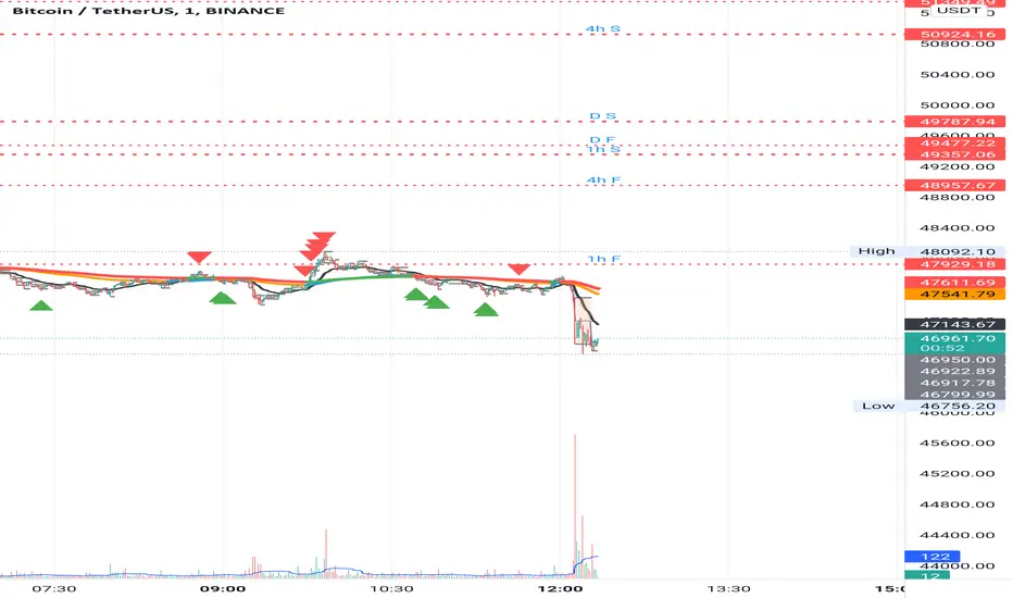
EMA MTF PlusI like trading the 1 minute and 3 minutes time-frames. I'm what is commonly called a "scalper". Long term investments yes, I have some, but for trading, I don't have neither the time,
nor the patience to wait hours or days for my trade to be complete.
This doesn't mean I discount the higher time-frames, no, I actually rely heavily on them. I found that EMAs do a decent job as support/resistance, sometimes to a tick level of precision. And this is important for a 1 minute trader.
As such, I made this script that tracks the higher time-frames EMAs and displays the last value as a line.
I do not need the whole EMA, I'm not interested in crossovers or crossunders, these are anyway late signals for me.
What's with the triangles? These are local tops/bottoms , candles that have a have decent size of the wick. These tops and bottoms are by no means "final", they are merely a rejection at certain levels of price. Due to markets complexities (and human erratic behaviors hehe) these levels could be breached at the very next candle. For a more "final" version (nothing is really final but..) I added Schaff Trend Cycle as filter, so a triangle will pop only when a trend is mature enough ( STC with a value near 0 or near 100).
Colored bars. When the body of the candle is big, it shows strength. Strong bars tend to have follow through, especially when breaking key levels. The script looks at the body of the candle and compares it with ATR (Average True Range), if it's at least 0.8 of ATR it changes the bar color to yellow (bull candles) or fuchsia(bear candles).
Range identifier. This code is copied from Lazy Bear (if there are any issues please let me know), it's very useful in conjunction with colored bars.
I look for breakout candles that go outside of the range as a signal for a trade.
There are many ways in which this script can be useful, like trading mean reversions or momentum trades (breakouts) or simply trend following trades.
I hope you guys find it useful, you can play with default values and change them as you like, these are what I found to be working best for me and my trading universe (mostly crypto).
Special thanks for the original work of:
LazyBear
everget
Jim8080
Pythagorean Means of Moving AveragesDESCRIPTION
Pythagorean Means of Moving Averages
1. Calculates a set of moving averages for high, low, close, open and typical prices, each at multiple periods.
Period values follow the Fibonacci sequence.
The "short" set includes moving average having the following periods: 5, 8, 13, 21, 34, 55, 89, 144, 233, 377.
The "mid" set includes moving average having the following periods: 5, 8, 13, 21, 34, 55, 89, 144, 233, 377, 610, 987, 1597.
The "long" set includes moving average having the following periods: 5, 8, 13, 21, 34, 55, 89, 144, 233, 377, 610, 987, 1597, 2584, 4181.
2. User selects the type of moving average: SMA, EMA, HMA, RMA, WMA, VWMA.
3. Calculates the mean of each set of moving averages.
4. User selects the type of mean to be calculated: 1) arithmetic, 2) geometric, 3) harmonic, 4) quadratic, 5) cubic. Multiple mean calculations may be displayed simultaneously, allowing for comparison.
5. Plots the mean for high, low, close, open, and typical prices.
6. User selects which plots to display: 1) high and low prices, 2) close prices, 3) open prices, and/or 4) typical prices.
7. Calculates and plots a vertical deviation from an origin mean--the mean from which the deviation is measured.
8. Deviation = origin mean x a x b^(x/y)/c.
9. User selects the deviation origin mean: 1) high and low prices plot, 2) close prices plot, or 3) typical prices plot.
10. User defines deviation variables a, b, c, x and y.
Examples of deviation:
a) Percent of the mean = 1.414213562 = 2^(1/2) = Pythagoras's constant (default).
b) Percent of the mean = 0.7071067812 = = = sin 45˚ = cos 45˚.
11. Displaces the plots horizontally +/- by a user defined number of periods.
PURPOSE
1. Identify price trends and potential levels of support and resistance.
CREDITS
1. "Fibonacci Moving Average" by Sofien Kaabar: two plots, each an arithmetic mean of EMAs of 1) high prices and 2) low prices, with periods 5, 8, 13, 21, 34, 55, 89, 144, 233, 377, 610, 987, 1597, 2584, 4181.
2. "Solarized" color scheme by Ethan Schoonover.

Keltner Channels BandsKeltner Channel Bands
Great indicator for mean reversion strategies.
Alerts you can set:
Crossover EMA
Crossunder EMA
Crossover upper band
Crossunder upper band
Crossover lower band
Crossunder lower band
Have fun!

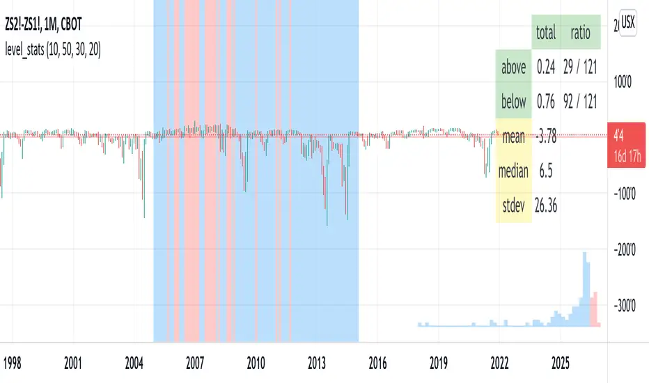
level_statsThis script tells you the percentage of time an instrument's closing value is above and below a level of your choosing. The background color visually indicates periods where the instrument closed at or above the level (red) and below it (blue). For "stationary-ish" processes, you can get a loose feel for the mean, high, and low values. The historical information conveyed through the background coloring can help you plan derivatives trades. Try with your favorite pairs, commodities, or volatility indices.
Usage: pick a level of interest using the input.
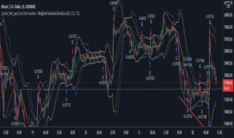
[cache_that_pass] 1m 15m Function - Weighted Standard DeviationTradingview Community,
As I progress through my journey, I have come to the realization that it is time to give back. This script isn't a life changer, but it has the building blocks for a motivated individual to optimize the parameters and have a production script ready to go.
Credit for the indicator is due to @rumpypumpydumpy
I adapted this indicator to a strategy for crypto markets. 15 minute time frame has worked best for me.
It is a standard deviation script that has 3 important user configured parameters. These 3 things are what the end user should tweak for optimum returns. They are....
1) Lookback Length - I have had luck with it set to 20, but any value from 1-1000 it will accept.
2) stopPer - Stop Loss percentage of each trade
3) takePer - Take Profit percentage of each trade
2 and 3 above are where you will see significant changes in returns by altering them and trying different percentages. An experienced pinescript programmer can take this and build on it even more. If you do, I ask that you please share the script with the community in an open-source fashion.
It also already accounts for the commission percentage of 0.075% that Binance.US uses for people who pay fees with BNB.
How it works...
It calculates a weighted standard deviation of the price for the lookback period set (so 20 candles is default). It recalculates each time a new candle is printed. It trades when price lows crossunder the bottom of that deviation channel, and sells when price highs crossover the top of that deviation channel. It works best in mid to long term sideways channels / Wyckoff accumulation periods.
MomentsLibrary "Moments"
Based on Moments (Mean,Variance,Skewness,Kurtosis) . Rewritten for Pinescript v5.
logReturns(src) Calculates log returns of a series (e.g log percentage change)
Parameters:
src : Source to use for the returns calculation (e.g. close).
Returns: Log percentage returns of a series
mean(src, length) Calculates the mean of a series using ta.sma
Parameters:
src : Source to use for the mean calculation (e.g. close).
length : Length to use mean calculation (e.g. 14).
Returns: The sma of the source over the length provided.
variance(src, length) Calculates the variance of a series
Parameters:
src : Source to use for the variance calculation (e.g. close).
length : Length to use for the variance calculation (e.g. 14).
Returns: The variance of the source over the length provided.
standardDeviation(src, length) Calculates the standard deviation of a series
Parameters:
src : Source to use for the standard deviation calculation (e.g. close).
length : Length to use for the standard deviation calculation (e.g. 14).
Returns: The standard deviation of the source over the length provided.
skewness(src, length) Calculates the skewness of a series
Parameters:
src : Source to use for the skewness calculation (e.g. close).
length : Length to use for the skewness calculation (e.g. 14).
Returns: The skewness of the source over the length provided.
kurtosis(src, length) Calculates the kurtosis of a series
Parameters:
src : Source to use for the kurtosis calculation (e.g. close).
length : Length to use for the kurtosis calculation (e.g. 14).
Returns: The kurtosis of the source over the length provided.
skewnessStandardError(sampleSize) Estimates the standard error of skewness based on sample size
Parameters:
sampleSize : The number of samples used for calculating standard error.
Returns: The standard error estimate for skewness based on the sample size provided.
kurtosisStandardError(sampleSize) Estimates the standard error of kurtosis based on sample size
Parameters:
sampleSize : The number of samples used for calculating standard error.
Returns: The standard error estimate for kurtosis based on the sample size provided.
skewnessCriticalValue(sampleSize) Estimates the critical value of skewness based on sample size
Parameters:
sampleSize : The number of samples used for calculating critical value.
Returns: The critical value estimate for skewness based on the sample size provided.
kurtosisCriticalValue(sampleSize) Estimates the critical value of kurtosis based on sample size
Parameters:
sampleSize : The number of samples used for calculating critical value.
Returns: The critical value estimate for kurtosis based on the sample size provided.

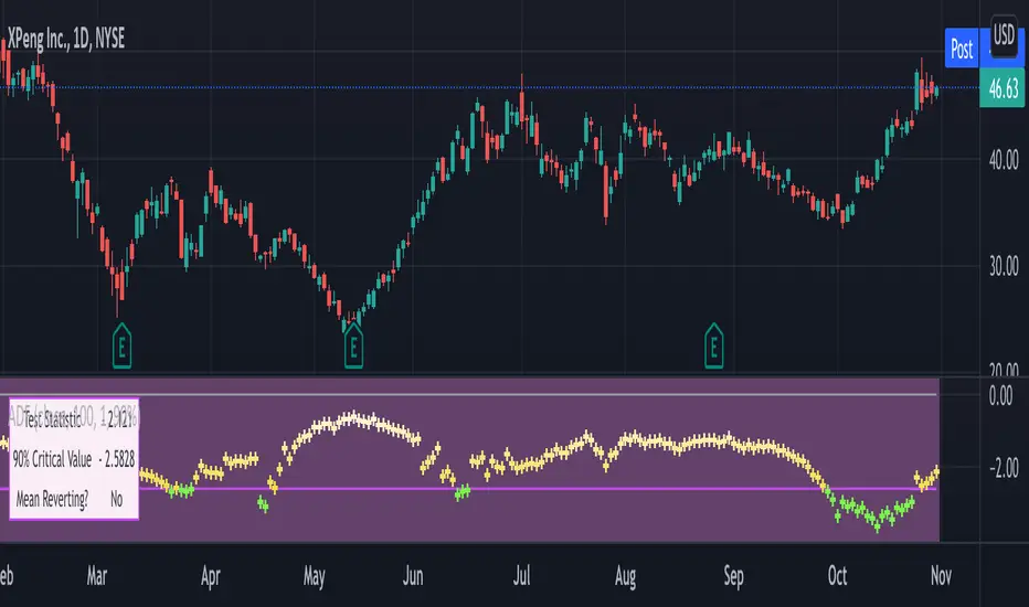
Augmented Dickey–Fuller (ADF) mean reversion testThe augmented Dickey-Fuller test (ADF) is a statistical test for the tendency of a price series sample to mean revert .
The current price of a mean-reverting series may tell us something about the next move (as opposed, for example, to a geometric Brownian motion). Thus, the ADF test allows us to spot market inefficiencies and potentially exploit this information in a trading strategy.
Mathematically, the mean reversion property means that the price change in the next time period is proportional to the difference between the average price and the current price. The purpose of the ADF test is to check if this proportionality constant is zero. Accordingly, the ADF test statistic is defined as the estimated proportionality constant divided by the corresponding standard error.
In this script, the ADF test is applied in a rolling window with a user-defined lookback length. The calculated values of the ADF test statistic are plotted as a time series. The more negative the test statistic, the stronger the rejection of the hypothesis that there is no mean reversion. If the calculated test statistic is less than the critical value calculated at a certain confidence level (90%, 95%, or 99%), then the hypothesis of a mean reversion is accepted (strictly speaking, the opposite hypothesis is rejected).
Input parameters:
Source - The source of the time series being tested.
Length - The number of points in the rolling lookback window. The larger sample length makes the ADF test results more reliable.
Maximum lag - The maximum lag included in the test, that defines the order of an autoregressive process being implied in the model. Generally, a non-zero lag allows taking into account the serial correlation of price changes. When dealing with price data, a good starting point is lag 0 or lag 1.
Confidence level - The probability level at which the critical value of the ADF test statistic is calculated. If the test statistic is below the critical value, it is concluded that the sample of the price series is mean-reverting. Confidence level is calculated based on MacKinnon (2010) .
Show Infobox - If True, the results calculated for the last price bar are displayed in a table on the left.
More formal background:
Formally, the ADF test is a test for a unit root in an autoregressive process. The model implemented in this script involves a non-zero constant and zero time trend. The zero lag corresponds to the simple case of the AR(1) process, while higher order autoregressive processes AR(p) can be approached by setting the maximum lag of p. The null hypothesis is that there is a unit root, with the alternative that there is no unit root. The presence of unit roots in an autoregressive time series is characteristic for a non-stationary process. Thus, if there is no unit root, the time series sample can be concluded to be stationary, i.e., manifesting the mean-reverting property.
A few more comments:
It should be noted that the ADF test tells us only about the properties of the price series now and in the past. It does not directly say whether the mean-reverting behavior will retain in the future.
The ADF test results don't directly reveal the direction of the next price move. It only tells wether or not a mean-reverting trading strategy can be potentially applicable at the given moment of time.
The ADF test is related to another statistical test, the Hurst exponent. The latter is available on TradingView as implemented by balipour , QuantNomad and DonovanWall .
The ADF test statistics is a negative number. However, it can take positive values, which usually corresponds to trending markets (even though there is no statistical test for this case).
Rigorously, the hypothesis about the mean reversion is accepted at a given confidence level when the value of the test statistic is below the critical value. However, for practical trading applications, the values which are low enough - but still a bit higher than the critical one - can be still used in making decisions.
Examples:
The VIX volatility index is known to exhibit mean reversion properties (volatility spikes tend to fade out quickly). Accordingly, the statistics of the ADF test tend to stay below the critical value of 90% for long time periods.
The opposite case is presented by BTCUSD. During the same time range, the bitcoin price showed strong momentum - the moves away from the mean did not follow by the counter-move immediately, even vice versa. This is reflected by the ADF test statistic that consistently stayed above the critical value (and even above 0). Thus, using a mean reversion strategy would likely lead to losses.
Pythagorean Moving Averages (and more)When you think of the question "take the mean of this dataset", you'd normally think of using the arithmetic mean because usually the norm is equal to 1; however, there are an infinite number of other types of means depending on the function norm (p).
Pythagoras' is credited for the main types of means: his harmonic mean, his geometric mean, and his arithmetic mean:
Harmonic Average (p = -1):
- Take the reciprocal of all the numbers in the dataset, add them all together, divide by the amount of numbers added together, then take the reciprocal of the final answer.
Geometric Average (p = 0):
- Multiply all the numbers in the dataset, then take the nth root where n is equal to the amount of number you multiplied together.
Arithmetic Mean (p = 1):
- Add all the numbers in the dataset, then divide by the amount of numbers you added by.
A couple other means included in this script were the quadratic mean (p = 2) and the cubic mean (p = 3).
Quadratic Mean (p = 2):
- Square every number in the dataset, then divide by the amount of numbers your added by, then take the square root.
Cubic Mean (p = 3):
- Cube every number in the dataset, then divide by the amount of numbers you added by, then take the cube root.
There are an infinite number of means for every scenario of p, but they begin to follow a pattern after p = 3.
Read more:
www.cs.uni.edu
en.wikipedia.org
en.wikipedia.org
Note : I added the functions for the quadratic mean and cubic mean, but since market charts don't have those types of graphs, the functions don't usually work. It's the same reason why sometimes you'll see the harmonic average not working.
Disclaimer : This is not financial or mathematical advice, please look for someone certified before making any decisions.

Hophop Reversion Strategy
█ OVERVIEW
Mean reversion is a financial term assuming that an asset's price will tend to converge to the average price over time.
Due to the trending nature of the crypto markets, mean reversion on a high timeframe could be pretty dangerous. When it comes to running mean reversion strategy on low timeframe, commission and slippage may cost more than strategy gains.
In this strategy, I tried to achieve being conservative in the trending market while avoiding trades if necessary and trading high probability reversion opportunities .
█ CONCEPTS
Strategy is build based on the combination of the momentum and the historical / implied volatility; when the price exceeds the potential volatility range, the strategy places the orders, and the target point is the mean of the expected range high and range low.
The range low and high lines displayed on the chart shows where to short or long, to make sure that the orders are limit orders; orders are placed 0.5% above/below the ranges!
Key information about the strategy
• All the orders are limit entry
• 0.02% commission is included in the backtest
• 30 ticks set for Verify Price Limit for Orders
• 30 ticks set for Slippage
• Initial version does not include the money management and hard stops hence you need to be extra cautious in trending markets
• Restricted to be used for BTC and ETH for 15 min timeframe
█ Ozet
Ortalamaya dönme, bir varlığın fiyatının zaman içinde ortalama fiyata yakınsama eğiliminde olacağını varsayan bir finansal terimdir.
Kripto piyasalarının trend egilimli doğası nedeniyle, yüksek zaman diliminde ortalamaya dönüş oldukça tehlikeli olabilir.
Ortalama geri dönüş stratejisini düşük zaman diliminde calistirmak söz konusu olduğunda, komisyon ve kayma, strateji kazanımlarından daha pahalıya mal olabilir.
Bu stratejide, gerektiğinde alım satımlardan kaçınırken ve yüksek olasılıklı ortalamaya dönüş fırsatlarını degerlendiren, trend olan piyasada ise isleme girerken temkinli olmasi uzerine calistim
█ Aciklama
Strateji, momentum ve tarihsel / zımni oynaklığın birleşimine dayalı olarak inşa edilmistir; fiyat potansiyel oynaklık aralığını aştığında, strateji emirleri verir ve hedef nokta, beklenen yüksek aralığın ve düşük aralığın ortalamasıdır.
Grafikte görüntülenen aralık alt ve üst satırları,
Stratejiye ait onemli bilgiler/b]
• Tüm emirler limit emirdir girişlidir
• Backtest performansinda %0.02 komisyon dahildir
• Limit Emir fiyat dogrulamasi icin 30 tick bekleme kullanilmistir
• Slippage için 30 tick bekleme kullanilmistir
• İlk sürüm para yönetimini ve stoploss içermez, bu nedenle trend olan piyasalarda ekstra dikkatli olmanız gerekir.
• 15 dakikalık zaman dilimi ile BTC ve ETH için kullanımla sınırlıdır
Emirlerin limit emir olduğundan emin olmak için nerede short veya long isleme girilecegini gosteren cizgilerin %0.5 üstünde/altında verilir!

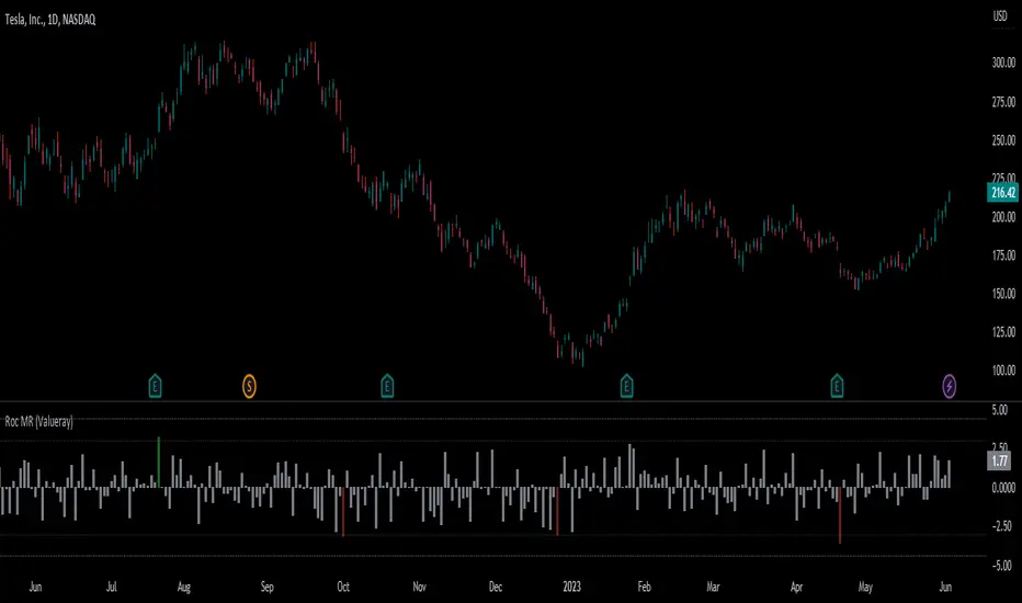
Roc Mean Reversion (ValueRay)This Indicator shows the Absolute Rate of Change in correlation to its Moving Average.
Values over 3 (gray dotted line) can savely be considered as a breakout; values over 4.5 got a high mean-reverting chance (red dotted line).
This Indicator can be used in all timeframes, however, i recommend to use it <30m, when you want search for meaningful Mean-Reverting Signals.
Please like, share and subscribe. With your love, im encouraged to write and publish more Indicators.
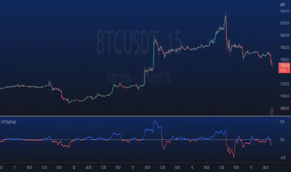
Drift Study (Inspired by Monte Carlo Simulations with BM) [KL]Inspired by the Brownian Motion ("BM") model that could be applied to conducting Monte Carlo Simulations, this indicator plots out the Drift factor contributing to BM.
Interpretation : If the Drift value is positive, then prices are possibly moving in an uptrend. Vice versa for negative drifts.
Alpha Trading - Deviation Log Pro - Coder WolvesAlpha Trading - Deviation Log Pro
Here at Alpha Trading we love our indicators built on returns. In our view, the only way to play divergences in Trading is divergences between Returns based oscillators and Price.
The Alpha Trading Deviation Log Pro displays a mean of log returns, with returns and price both weighted using our proprietary root mean square (RMS) Z-Score.
We also show standard error and confidence intervals.
Within the indicator settings, you can apply alerts to the RMS Z Score, as well as an option to turn on triangle and square shapes to assist with showing potential buy/sell and get out of trade signals.
Things to Understand First
Standard Error
The term "standard error" is used to refer to the standard deviation of various sample statistics, such as the mean or median. For example, the "standard error of the mean" refers to the standard deviation of the distribution of sample means taken from a population. The smaller the standard error, the more representative the sample will be of the overall population.
The relationship between the standard error and the standard deviation is such that, for a given sample size, the standard error equals the standard deviation divided by the square root of the sample size. The standard error is also inversely proportional to the sample size; the larger the sample size, the smaller the standard error because the statistic will approach the actual value.
The standard error is considered part of inferential statistics. It represents the standard deviation of the mean within a dataset. This serves as a measure of variation for random variables, providing a measurement for the spread. The smaller the spread, the more accurate the dataset.
Confidence Interval
A confidence interval is a range of values where an unknown population parameter is expected to lie most of the time, if you were to repeat your study with new random samples.
With a 95% confidence level, 95% of all sample means will be expected to lie within a confidence interval of ± 1.96 standard errors of the sample mean.
Settings
• Confidence Intervals plotted with Green and Red Horizontal Lines
• Standard Error Mean - Plotted as a blue dots
• Standard Error Upper - Plotted as a grey line
• Standard Error Lower -Plotted as grey line
• RMS Z-Score Alerts shown as Red and Green Dots
• Potential Buy Signal Green Triangle Up
• Potential Sell Signal - Red Triangle Down
• Get out of Long Trade - White Square
• Get Out of Short Trade - White Square
The Chart below is showing the Divergences between Returns and Price Action over a long term trend of a time series, no matter the time frame.
