Time Pressure ZonesTime Pressure Zones is a multi‑purpose candle and volume‑based indicator that highlights moments when markets are likely being driven by urgency rather than routine trading flow.
**Overview**
Detects sequences of strong, one‑directional candles accompanied by volume spikes to approximate institutional time pressure (forced buying or selling).
Paints subtle background zones, labels, and a net‑pressure histogram so you can see when aggressive flow is building or exhausting across any instrument and timeframe.
**Core Logic**
A bar is tagged “strong” when its real body occupies at least a user‑defined percentage of the full high‑low range, filtering out indecision candles and long‑wick noise.
Volume is compared to a rolling 20‑bar average; only bars with volume above a configurable multiple are treated as meaningful participation, which makes the tool adapt to different symbols and sessions.
The script counts consecutive bars that are both strong and high‑volume in the same direction, then flags a time‑pressure event once a set fraction of the lookback has been reached (e.g., 2 out of 3, 3 out of 5).
**Visual Outputs**
Background shading: green or red bands mark active bullish or bearish time‑pressure windows without overpowering other tools on the chart.
On‑chart labels: “↑ Time Pressure” and “↓ Time Pressure” appear only on the first bar of a new pressure sequence, ideal for alerts and discretionary entries.
Net Pressure histogram: plots the difference between bullish and bearish streak counts, giving a quick at‑a‑glance sense of which side currently dominates.
**Sessions and News**
Uses UTC‑based logic to highlight London and New York open and close windows, where institutional flows and intraday “deadline” behavior tend to cluster.
Includes a manual News Window toggle so you can mark high‑impact event periods (CPI, FOMC, NFP, etc.), aligning tape‑based urgency with scheduled catalysts.
**How To Use**
Look to join moves when fresh time‑pressure labels print into session opens, breakouts, or key levels, rather than fading them.
Tune the three main inputs per market and timeframe: lower thresholds for choppy or thin markets, and higher body/volume requirements for very liquid symbols like major indices or BTC pairs.
ZAMAN

NineThirtyNineThirty
Description:
NineThirty draws a vertical line at any user-specified time, helping traders visually track important moments on a chart. It includes built-in alerts and pre-alerts, making it easy to receive notifications exactly when a target time is reached or minutes before. Fully customizable and compatible with all markets and timeframes.
Features:
Draws a vertical line at any user-defined time.
Customize line color, style (solid, dotted, dashed), and width.
Supports multiple timezones, including Exchange, UTC, and major global markets.
Option to show only the most recent line for a cleaner chart.
Alerts at the target time, with optional pre-alerts minutes in advance.
Use Cases:
Track key times for trading strategies or session opens.
Receive alerts when important moments occur without constantly watching the chart.
Combine with other indicators for time-based analysis across any market or timeframe.


NYC Midnight LITE [Takeda Trades 2026]NYC Midnight LITE
by @TakedaTradesOfficial
v1 01/09/2026
═══════════════════════════════════════════════════════════════
NYC Midnight LITE Indicator
What This Indicator Does
This is a NYC Midnight Opening Range indicator that tracks the first hour of trading (00:00 - 01:00 EST) and uses it to identify potential trading opportunities throughout the day.
Core Concept
The indicator is based on the premise that the first hour of the New York trading day (midnight EST) establishes key price levels that often act as support/resistance for the remainder of the session. This is a popular ICT (Inner Circle Trader) concept.
═══════════════════════════════════════════════════════════════
Visual Elements Explained
1. Yellow Box (Hour 1 Range)
• Shows the HIGH and LOW established during 00:00-01:00 EST
• The box stops at the end of Hour 1
• The HIGH and LOW lines extend to current price for easy reference
2. Yellow Dashed Line (Midline)
• The middle point between Hour 1 high and low
• Often acts as a pivot - price may reverse here or use it as support/resistance
3. Black Lines (Open & Close)
• First line: The OPEN price of the very first candle at 00:00
• Second line: The CLOSE price of the very first candle
• These show immediate directional bias
4. Orange Vertical Line
• Marks the start of each new trading day at midnight EST
• Helps you identify session boundaries
5. Candle Colors
• Yellow candles: Currently in Hour 1 (00:00-01:00)
• Green candles: Price above Hour 1 high (bullish breakout)
• Red candles: Price below Hour 1 low (bearish breakout)
• Gray candles: Price inside Hour 1 range (consolidation)
═══════════════════════════════════════════════════════════════
How to Trade With This Indicator
Strategy 1: Breakout Trading (Most Common)
LONG Setup:
1. Wait for Hour 1 to complete (01:00 EST)
2. Enter when price closes above the yellow Hour 1 HIGH
3. Stop loss: Below Hour 1 low or midline
4. Target: Previous day high, or 1.5-2x the Hour 1 range
SHORT Setup:
1. Wait for Hour 1 to complete
2. Enter when price closes below the yellow Hour 1 LOW
3. Stop loss: Above Hour 1 high or midline
4. Target: Previous day low, or 1.5-2x the Hour 1 range
Tips:
• Stronger breakouts often happen during London session (2:00-5:00 EST) or NY open (9:30 EST)
• Use the alerts to notify you when breakouts occur
─────────────────────────────────────────────────────────────
Strategy 2: Range Reversion (Contrarian)
If price breaks out but lacks momentum:
• Wait for price to reenter the Hour 1 range
• Trade back toward the midline or opposite boundary
• Best during low-volatility sessions
─────────────────────────────────────────────────────────────
Strategy 3: Midline Bounce
The yellow dashed midline often acts as support/resistance:
• If price is above midline: Look for bounces off midline to go long
• If price is below midline: Look for rejections at midline to go short
• Works well during choppy/ranging days
─────────────────────────────────────────────────────────────
Strategy 4: First Candle Bias
The black lines (first candle open/close) show early directional intent:
• Close > Open: Bullish bias - favor longs on pullbacks
• Close < Open: Bearish bias - favor shorts on rallies
• These lines often act as intraday support/resistance
═══════════════════════════════════════════════════════════════
Best Practices
Timeframes
• Best on: 1-minute, 5-minute, 15-minute charts
• The indicator tracks NYC time, so it works on any timezone
Markets
• Forex pairs: EUR/USD, GBP/USD, USD/JPY (high liquidity)
• Indices: ES, NQ futures, SPY (active during NYC session)
• Crypto: BTC, ETH (24/7 markets with strong NYC midnight volatility)
Risk Management
• The Hour 1 range gives you natural stop-loss levels
• Risk 1-2% per trade
• If the range is very small (<10 pips/points), wait for expansion
═══════════════════════════════════════════════════════════════
What the Settings Mean
• Show Hour 1 Box: Displays the yellow range box
• Show Midline: Shows the dashed middle line
• Color Hour 1 Candles Yellow: Highlights the first hour
• Color Candles Based on Range: Green/Red/Gray based on position
• Show Labels: Displays "NYC 00:00" marker
• Box Transparency: Adjust visibility of the yellow box
═══════════════════════════════════════════════════════════════
Common Scenarios
Bullish Day Example:
• Hour 1 range forms: High at 4500, Low at 4480
• At 3:00 EST, price breaks above 4500 (green candles)
• Enter long, stop at 4490 (midline), target 4530
Bearish Day Example:
• Hour 1 range: High 1.0850, Low 1.0830
• Price breaks below 1.0830 at London open
• Enter short, stop at 1.0840 (midline), target 1.0810
Ranging Day Example:
• Small Hour 1 range forms
• Price chops between high/low all day (gray candles)
• Avoid breakout trades - fade extremes back to midline instead
═══════════════════════════════════════════════════════════════
Key Takeaways
✅ Wait for Hour 1 to complete before making decisions
✅ Clean breaks with strong candles are more reliable
✅ Combine with other confluences (support/resistance, market structure)
✅ The midline is your friend - watch for reactions there
✅ Alerts will notify you of breakouts automatically
This is a framework, not a crystal ball. Use proper risk management and combine with your trading plan!

Trading Sessions The sessions are individually selectable, meaning you can choose which sessions you want to display.
There is also a legend in the bottom left showing the corresponding trading hours.
Displayed sessions:
ASIA
LONDON
NEW YORK
#ZEBI

Key Time LevelsThis script draws horizontal lines on the chart at important New York trading times so you can see where price opened and reacted during the day. It marks the ETH open, midnight, 3:00 AM, 8:30 AM, 9:30 AM, and 10:00 AM using NY time so daylight savings doesn’t mess it up. Each line starts exactly when that time happens and stops at the 4:00 PM close, so nothing carries into the next day. It keeps past days on the chart so you can look back and see how price reacted at those levels. Basically, it helps you see time-based levels that matter without cluttering the chart.

Ultimate Time & Countdown v1.5 - Pro Borderif you are interested to use my script. please comment below or send me a message

Passiv Algo V2 PXL PXH Time-Based Liquidity Levels Indicator
This indicator automatically identifies and plots time-based liquidity levels derived from key market sessions and higher-timeframe reference periods.
By focusing on institutional trading windows and recurring time structures, it highlights areas where liquidity is statistically more likely to be present — zones that often act as reaction points with a high probability of price rejection or reversal.
Key Features:
🔹Automatic detection of time-based liquidity levels
🔹Levels based on previous session highs & lows and intraday reference ranges
🔹Designed to align with institutional market timing
🔹Clean and non-repainting levels
🔹Works on all markets and timeframes
Why it works:
Financial markets move in cycles driven by time and liquidity. When price revisits liquidity pools formed at specific times, it often reacts due to order accumulation and distribution by large participants. This indicator helps traders anticipate those reactions before price reaches the level.
Best Use Cases:
🔹Liquidity sweeps & rejections
🔹Mean reversion setups
🔹Session-based trading strategies
🔹Confluence with market structure and price action
⚠️ This indicator does not provide trade signals. It is designed to be used as a contextual tool alongside proper risk management and confirmation.

Gann Sacred Geometry Hexagram Ver 1.0# **Gann Sacred Geometry Hexagram Ver 1.0**
### **Advanced Gann Theory with Sacred Geometry Confluence Signals**
---
## ** Background:**
**W.D. Gann (1878-1955)** was one of the most legendary traders in history, reportedly achieving over 90% trading accuracy. He discovered that markets don't move randomly—they follow geometric and mathematical laws encoded in nature itself.
Gann spent years studying:
- **Ancient Egyptian geometry and pyramids**
- **Pythagorean mathematics** (sacred ratios)
- **Biblical numerology and Hebrew Kabbalah**
- **Astronomical cycles and planetary movements**
- **Musical harmonics and octaves**
His core discovery: **"When time and price square, expect a market change."**
### **Sacred Geometry in Markets:**
The **Hexagram (Star of David)** represents perfect market balance:
- **△ Triangle Up** = Bullish forces, Yang energy, Fire element, Expansion
- **▽ Triangle Down** = Bearish forces, Yin energy, Water element, Contraction
- **Together (🔯)** = Market equilibrium—where opposing forces meet
When price reaches these geometric intersections at precise time intervals, major reversals or continuations occur.
### **Gann's Key Principles:**
1. **Price-Time Balance** - Markets must balance price movement with time elapsed
2. **Geometric Angles** - Price moves along predictable geometric rays (45°, steeper, shallower)
3. **Square of Nine** - Markets move in "squares" completing geometric cycles
4. **Harmonic Divisions** - 8ths, quarters, halves—like musical octaves—mark turning points
5. **Cardinal Cross** - 0%, 25%, 50%, 75%, 100% are magnetically important levels
**Gann's Philosophy:**
> "Markets are based on natural law. What has occurred before will occur again because markets operate on cycles. Understanding geometry and time unlocks market behavior."
---
## **What This Indicator Does:**
This script translates Gann's complex theories into visual, actionable trading signals by:
1. **Creating a geometric grid** based on major swings (Square of Nine principle)
2. **Overlaying sacred hexagram patterns** at key price-time zones
3. **Calculating all 9 Gann angles** dynamically as support/resistance
4. **Detecting confluence** when multiple Gann principles align simultaneously
5. **Generating high-probability signals** with scoring (0-30 points)
When price touches multiple geometric levels + angles + time cycles + trend alignment = **Maximum Gann Confluence** 🎯
---
## **Core Methodology:**
**Gann Principles Implemented:**
- **9 Gann Angles** (1x1, 2x1, 1x2, 3x1, 1x3, 4x1, 1x4, 8x1, 1x8)
- 1x1 (45°) is the "Master Angle"—most important
- Steeper/shallower angles provide support/resistance layers
- **Cardinal Cross Levels** (0%, 25%, 50%, 75%, 100%)
- 50% level = center of gravity (most powerful)
- Quarter divisions mark psychological/geometric zones
- **Gann's 8ths Timing** - Markets turn at 1/8, 1/4, 3/8, 1/2, 5/8, 3/4, 7/8 of cycle
- Based on musical octaves and harmonic vibrations
- **Price-Time Squaring**
- When price moved = time elapsed → market is "squared" → change imminent
- **Square of Nine Grid**
- Geometric cells extending forward in time
- Each cell = complete price-time cycle
**Sacred Geometry Elements:**
- **Hexagram Pattern** (Star of David) - Balance of opposing forces
- **Golden Ratio (Phi 1.618)** - Nature's proportion in market structure
- **Geometric Confluence Zones** - Where multiple patterns intersect
---
## **How Signals Are Generated:**
**Buy Signals** occur when multiple confirmations align:
- ✅ Price touches **downward Gann angles** (support)
- ✅ Near **Cardinal Cross levels** (especially 50%)
- ✅ At **Gann 8th cycle divisions** (timing)
- ✅ **Price-time relationship is squared** (balanced)
- ✅ **3+ angles cluster together** (confluence zone)
- ✅ **Aligned with uptrend** (optional filter)
**Sell Signals** trigger when:
- ✅ Price touches **upward Gann angles** (resistance)
- ✅ At geometric levels during cycle timing
- ✅ Multiple Gann principles converge
**Confluence Scoring (0-30 points):**
| Element | Points | Meaning |
|---------|--------|---------|
| 50% Cardinal Level | 6 | Center of gravity |
| 3+ Angle Cluster | 6 | Strong confluence |
| 1x1 Master Angle | 5 | Most important angle |
| 0%/100% Boundaries | 5 | Square edges |
| Price-Time Squared | 4 | Gann balance |
| Gann 8th Timing | 3 | Cycle turning point |
| Trend Alignment | 3 | Direction confirmation |
**Higher score = Stronger confluence = Higher probability setup**
Default minimum: 12 points (customizable 8-30)
---
## **Key Features:**
### **Visual Elements:**
✅ Square grid cells (Square of Nine)
✅ Hexagram overlays (Star of David sacred geometry)
✅ Golden ratio inner triangles (Phi 1.618)
✅ 9 Gann angle projections
✅ Cardinal Cross levels (0-25-50-75-100%)
✅ Extended price levels into future
✅ Time cycle divisions
✅ All elements toggle on/off
### **Signal Controls:**
✅ Minimum confluence score (8-30, default: 12)
✅ Price/angle tolerance adjustments
✅ Signal cooldown periods
✅ Boundary requirement filters
✅ Trend alignment (EMA-based)
✅ Counter-trend signal toggle
✅ Gann 8ths timing on/off
✅ Price-Time Square filter
✅ Angle clustering detection
### **Customization:**
✅ Gann numbers: 11, 22, 44, 88, 176, 352 (harmonic choices)
✅ Grid size: 1x1 to 7x7
✅ Line thickness controls
✅ Color schemes
✅ Signal display styles (Labels, Diamonds, Circles, Stars)
✅ Confluence score display on/off
### **Alert System:**
✅ Built-in TradingView alerts
✅ Real-time signal notifications
✅ Custom alert messages
---
## **Best Use Cases:**
📊 **Swing Trading** - Identify key reversal zones days in advance
⏰ **Time Cycle Analysis** - Predict turning points with 8ths divisions
📈 **Trend Trading** - Gann angles show dynamic support in trends
🎯 **Confluence Trading** - Multiple confirmations reduce false signals
⚖️ **Balance Point Trading** - Find where price-time squares
**Optimal Timeframes:** 1H, 4H, Daily (works on all timeframes)
---
## **Settings Guide:**
**Conservative Approach (Higher Accuracy):**
- Min Confluence Score: 15+
- Trend Filter: ON
- Require Boundary: ON
- Allow Counter-Trend: OFF
- Price-Time Square: ON
**Aggressive Approach (More Signals):**
- Min Confluence Score: 10-12
- Trend Filter: Optional
- Allow Counter-Trend: ON
- Price-Time Square: Optional
**Recommended Starting Settings:**
- Gann Number: 88 (harmonic choice)
- Grid Size: 3x3 (balanced view)
- Min Score: 12 (good confluence)
- Trend Filter: ON (safer)
---
## **Important Disclaimers:**
⚠️ **Educational Tool** - Based on historical Gann principles. Not financial advice.
⚠️ **Learning Curve** - Sacred geometry and Gann analysis are advanced concepts. Study the patterns before live trading.
⚠️ **Risk Management** - Always use stop losses and position sizing. No indicator is 100% accurate.
⚠️ **Best Combined With:**
- Market structure understanding
- Your own trading strategy
- Fundamental analysis
⚠️ **Market Conditions** - Works best in trending markets with clear swings. Less effective in choppy, range-bound conditions.
---
## **How to Use:**
1. **Let Grid Form** - Wait for major swing high-to-low to establish grid
2. **Watch Confluences** - Look for signals with scores 12+
3. **Confirm Direction** - Use trend filter or check higher timeframe
4. **Enter on Signal** - Buy/Sell labels appear at confluence zones
5. **Manage Risk** - Set stops at opposite grid levels
6. **Target Next Level** - Grid shows natural targets at cardinal levels
**Pro Tip:** Higher confluence scores (18+) = exceptional setups. Wait for these!
---
## **Version History:**
**Version 1.0** - Initial Release
- Complete 9-angle Gann system
- Cardinal Cross levels (0-25-50-75-100%)
- Gann 8ths harmonic timing
- Price-Time Square detection
- Angle clustering confluence
- Trend alignment filters
- Hexagram sacred geometry overlay
- Golden ratio (Phi) triangles
- Customizable scoring system
---
**Gann's Final Wisdom:**
> "The future is but a repetition of the past. Study the past to know the future. The market moves in circles and cycles because human nature never changes."
---
**Trade with geometry. Trade with time. Trade with Gann.** 🎯🔯📐

Quarterly Theory - Daily CyclesQuarterly Theory - Daily Cycles
Automatically divides the trading day into four 6-hour quarters based on Quarterly Theory:
Q1: 6pm - 12am (midnight)
Q2: 12am - 6am
Q3: 6am - 12pm (noon)
Q4: 12pm - 6pm
Features shaded boxes for each quarter, vertical divider lines at quarter boundaries, and clear labels. Resets daily at 6pm. Fully customizable colors, borders, and display options.

Power Hour Trendlines [LuxAlgo]The Power Hour Trendlines indicator is based on Power Hours detection, and includes up to three displayed trendlines derived from the closing prices of all the bars within the last user-selected Power Hours.
Users can edit the time of Power Hours, choose how many sessions to take into account, enable or disable any trendlines, and change their colors.
🔶 USAGE
The Power Hour is defined as the last hour of the trading session and is set by default from 3:00 p.m. to 4:00 p.m. New York time. During this period, volume and volatility enter the market. Traders using higher timeframes may use this period to enter or exit positions by placing MOC (Market on Close) orders.
This tool works under the hypothesis that prices made during power hours (periods with high trading activity) are more relevant when used for the construction of trendlines.
An initial trendline is fit using linear regression; prices from power hours located above this initial fit are used for the upper trendline, while the ones below the fit are used for the lower one.
As with any trendline, traders can analyze the slope to determine the market's direction:
Positive slope: The market is trending up.
Negative slope: The market is trending down.
No slope: The market is trending sideways.
As we can see in the image, Nasdaq and Bitcoin are clearly in downtrends, gold is clearly in an uptrend, and the euro/U.S. dollar is in a sideways market over the last visible sessions.
As you can see, the trend lines may or may not be parallel to each other. The wider the area, the more volatile the data. The narrower the area, the less volatile the data. Let's look at an example.
In the image, the Dow30 and the euro/U.S. dollar have opposite behaviors. The volatility above the middle trendline is growing in the first case but shrinking in the second. In both cases, the volatility in the bottom area seems steady, so there are no big surprises there.
Traders can adjust the number of sessions for calculations, making the tool ideal for analyzing price behavior over different time frames.
As the image shows, we can clearly see how the market behaves over different time periods. XLY has been moving down over the last 10, 20, and 40 sessions, with a steeper decline over shorter periods. However, it has been moving sideways over the last 70 sessions.
One of the main uses of trendlines is to provide key support and resistance. In the image, SPY is shown with trendlines over the last 20 sessions. These lines provide excellent reference points for trading and observing price behavior in those areas, such as whether prices are accepted or rejected, which may trigger a response from other traders.
🔹 Not Allowed Timeframes
For obvious reasons, timeframes larger than 1H are not allowed. The Power Hour is defined as the last hour of the trading session. The tool will display a warning message if the timeframe is longer than 60 minutes.
🔶 SETTINGS
Power Hour (NY Time): Choose a custom Power Hour in New York time
Sessions Memory: Select how many Power Hours to take into account for calculations.
🔹 Style
Top: Enable or disable the top line and choose the line and background colors.
Middle: Enable or disable the middle line and choose the line color.
Bottom: Enable or disable the bottom line and choose the line and background colors.
Background: Enable or disable the background color for top and bottom lines.

Seasonal Strategies V1Seasonal Strategies V1 is a rule-based futures seasonality framework built around predefined calendar windows per asset.
The strategy automatically detects the current symbol and activates long or short trading phases strictly based on historically observed seasonal tendencies. All entries and exits are fully time-based — no indicators, no predictions, no discretionary input.
Key Features
Asset-specific seasonal windows (MMDD-based)
Automatic long and short activation
Fully time-based entries and exits
One position at a time (no pyramiding)
Clean chart visualization using subtle background shading
No indicators, no filters, no curve fitting
Philosophy:
This strategy is designed as a structural trading tool, not a forecasting model.
It focuses on when a market historically shows seasonal tendencies — not why or how far price might move.
Seasonal Strategies V1 intentionally keeps the chart clean and minimal, making it suitable as a baseline framework for research, portfolio-style seasonal approaches, or further extensions in later versions.
Intended Use:
Futures and commodity markets
Seasonality research and testing
Systematic, calendar-driven strategies
Educational and analytical purposes
Disclaimer
This script is provided for educational and research purposes only.
Past seasonal tendencies do not guarantee future performance.
Risk management, position sizing, and portfolio decisions are the responsibility of the user.

Ichimoku + Time Theory Cluster PRO++ (ZZZ)## Ichimoku + Time Theory Cluster PRO++ (ZZZ)
### 1) What does this script do?
**Ichi+Time PRO++** combines **Ichimoku + Ichimoku Time Theory (Hosoda’s time cycles)** to:
- Automatically plot **Ichimoku (Tenkan/Kijun/Chikou/Kumo)** as a **trend filter & support/resistance framework**.
- Calculate **projected time targets** derived from **pivots (swing highs/lows)**, then **cluster** nearby targets into **“time windows”** where the probability of **reversal / acceleration / strong volatility** is higher than usual.
- Show **early warnings (countdown “~in N bars”)** and classify clusters as **Normal / Strong** using a **score**.
> Core idea: **Price can travel far/short based on “price”, but it often turns hard around certain “time” marks.** Ichimoku helps define *direction and key areas*, while Time Clusters tell you *when to be on alert*.
---
### 2) How it works (simple overview)
1. **Detect pivots** (swing highs/lows) using Pivot Left/Right
- A pivot is confirmed only after *pivRight* bars → less noise.
2. From each pivot, the script generates **projected time targets** based on Time Theory cycle offsets (bar intervals).
3. Nearby projections are **grouped into clusters** using **“Tolerance ± bars”**.
4. A cluster is kept only if it meets:
- **Min hits**: minimum number of projections inside the same window
- **Min score**: minimum score threshold
Score = **baseScore (weighted hits)** + **contextBonus (Ichimoku context)**
→ Clusters aligned with favorable Ichimoku conditions are **prioritized**.
---
### 3) What you will see on the chart
- **Ichimoku**: Tenkan / Kijun / Chikou / Kumo (to read trend & key zones).
- **Time Cluster Window**:
- **Normal**: meets baseline conditions.
- **Strong (TC++)**: higher score (≥ strongScore) → more important.
- **Tooltips / info labels** (e.g., hits, base, ctx, score, ~in N bars) show:
- How strong a cluster is
- How many bars remain until the “time window”
---
### 4) Practical usage (recommended workflow)
**Step 1 — Filter the trend with Ichimoku**
- Prefer Long when: price is **above Kumo**, Tenkan > Kijun, Chikou is not obstructed.
- Prefer Short when: price is **below Kumo**, Tenkan < Kijun, Chikou is not obstructed.
**Step 2 — Use Time Clusters to pick the “WHEN”**
- When a **Time Cluster (Normal/Strong)** appears, interpret it as:
- A **“sensitive time window”** → higher chance of reversal, breakout, acceleration, or sharp shakeout.
- Not an automatic entry; you still need **price action confirmation**.
**Step 3 — Entry trigger**
- Wait for confirmation such as: structure break, pin/engulf candle, range breakout, Kijun/Kumo retest, etc.
- **Strong clusters** are often useful to:
- Hunt reversals around Ichimoku zones (Kijun/Kumo)
- Hunt breakouts when consolidating and Ichimoku agrees with the trend
**Step 4 — Risk management**
- Place SL using the nearest structure (swing/pivot/Kijun) + buffer.
- If already in a trade, Time Clusters can help you:
- tighten SL, take partial profits, or anticipate volatility.
---
### 5) Presets (A/B) & signal tuning
- **Mode A: “Fewer but stronger”**
Stricter filtering → fewer clusters, higher quality (swing/position-friendly).
- **Mode B: “More early warnings”**
Moderate filtering → more clusters (good for earlier monitoring and flexibility).
- **Custom**
Manually adjust key parameters:
- Pivot Left/Right
- Tolerance ± bars
- Min hits / Min score / Strong score
- Filter small pivots (reduce noise)
> Tip: Higher timeframes (4H–1D) usually work best with Mode A (cleaner). Lower timeframes (15m–1H) can use Mode B, but require disciplined triggers.
---
### 6) Important notes (avoid misinterpretation)
- Pivots require confirmation → pivot-based signals **do not print exactly at the top/bottom**, but after *pivRight* bars.
- Future **projected clusters may shift** when new pivots appear (they update with new data).
Treat Time Clusters as **time windows to be alert**, not “exact entry points”.
- This script does not replace a trading plan; always use proper position sizing and risk control.
---
### 7) Performance
This script uses many drawing objects (box/label/line). If your device is slow:
- Reduce **Max pivots stored**
- Reduce the number of clusters displayed or switch to **Mode A**
- Use a higher timeframe
---
**Disclaimer:** This tool is for technical analysis support only and is not financial advice. You are responsible for your own trading decisions.
---
## User Guide
### 1) What is this indicator for?
This indicator combines **Auto Ichimoku** + **Time Theory Clusters** to:
- Identify **trend & equilibrium zones** via Ichimoku (Kumo, Tenkan/Kijun, Chikou).
- Find **time windows** with higher probability of volatility/reversal/acceleration (Time Clusters).
- Score each time cluster based on **cluster strength (hits)** and **Ichimoku context (context bonus)**.
> Key reminder: Time Clusters answer **WHEN**, not **WHERE**. Always combine them with **price confirmation / Ichimoku / PA** before entering.
---
### 2) Add the indicator & quick setup
1. Open a chart → **Indicators** → choose **Ichimoku + Time Theory Cluster PRO++**.
2. Recommended timeframes:
- Swing/position: **H4 – D1 – W1**
- Intraday: **M15 – H1** (noisier; needs stricter filtering).
3. Choose **Mode (Preset)**:
- **A: Fewer but stronger** → stricter, fewer signals, higher quality (recommended for swing).
- **B: More early warnings** → more signals (recommended for intraday monitoring).
- **Custom** → fine-tune all parameters.
---
### 3) Signal meaning (how to read the chart)
The indicator marks **Time Clusters** in two levels:
- **Time Cluster Enter (Normal)**: meets minimum thresholds (minHits/minScore).
- **Time Cluster Enter (Strong / TC++)**: strong cluster (score ≥ strongScore) → higher priority.
**Correct interpretation:**
- As price approaches a Time Cluster window, the market is more likely to:
- reverse,
- break out of consolidation,
- accelerate a trend,
- or produce strong volatility (sweep/false break).
- Trading direction should be aligned with **Ichimoku context** (see section 4).
---
### 4) Suggested trading rules (practical & simple)
#### A. Trend trading (recommended)
**Prefer LONG when:**
- Price is **above Kumo**, future Kumo is bullish (Span A > Span B).
- Tenkan is **above** Kijun (or just crossed up), Chikou is not trapped by price/cloud.
- At a Time Cluster:
- Look for a **pullback** to Kijun/Tenkan or structural support,
- Wait for confirmation (engulfing/pinbar/micro-structure break),
- Enter.
**Prefer SHORT when:**
- Price is **below Kumo**, future Kumo is bearish (Span A < Span B).
- Tenkan is **below** Kijun, Chikou is pressured/blocked.
- At a Time Cluster:
- Look for a rally into Kijun/cloud edge,
- Wait for rejection, then enter.
✅ Tip: **Strong clusters (TC++)** matter most when they align with:
- Kumo edge,
- Kijun,
- horizontal S/R,
- supply/demand (order block) or swing high/low.
#### B. Reversal trading (only with strong confirmation)
Consider reversals only when:
- Time Cluster is **Strong (TC++)**
- + you see a **structure shift** (BOS/CHoCH) or a clear reversal candle setup,
- + Ichimoku shows weakness (price inside cloud, flat Tenkan/Kijun, Chikou trapped).
---
### 5) Risk management (mandatory)
- Do not enter just because you “reached a Time Cluster”.
- Always set SL by structure:
- LONG: below swing low / below Kijun / below nearest cloud edge.
- SHORT: above swing high / above Kijun / above nearest cloud edge.
- Take profit using:
- minimum R:R **1:1.5 – 1:2**
- or key targets (prior highs/lows, cloud boundaries, fib levels, etc.)
---
### 6) Inputs explained (Custom mode)
- **Pivot Left / Pivot Right**: pivot confirmation (higher = fewer but more reliable pivots).
- **Max pivots stored**: how many pivots are stored for clustering (more = more sensitive but heavier).
- **Tolerance ± bars**: cluster window width (larger = more clusters; smaller = sharper).
- **Min hits**: minimum overlaps to qualify as a cluster.
- **Min score**: minimum score to accept a cluster.
- **Strong score**: threshold to mark strong clusters (TC++).
- **Filter small pivots / Filter mode**: remove small pivots to reduce noise (recommended ON).
---
### 7) Alerts (recommended)
You can create alerts for:
- **Time Cluster Enter (Normal)**
- **Time Cluster Enter (Strong / TC++)**
Recommendation: set alerts on your main trading timeframe (H1/H4/D1) to avoid spam on very small TFs.
---
### 8) Disclaimer
This indicator is for technical analysis support only and is **not financial advice**. All trading decisions are your responsibility. Please test (forward/backtest) and apply risk management before using real money.
---
### 9) Access (Invite-only, if applicable)
To request access, send me a private message on TradingView with:
- TradingView username
- Market you trade (Crypto/FX/Indices…)
- Primary timeframe (e.g., H1/H4/D1)
I will grant access in order of requests.
---

Gann Octave Pro - Angles & Time Cycles 🎯 Gann Octave Pro - Angles & Time Cycles
## Complete Gann Trading System - Price, Angles & Time in One Indicator
A professional-grade Gann analysis tool combining **Octave Price Levels**, **Gann Angles (1x1, 2x1, 1x2)**, and **Advanced Time Cycle Projections**. Perfect for traders seeking precision market timing through geometric confluence.
---
## 🌟 Key Features
### 📐 Octave Price Levels
- **5 Key Levels**: 0%, 25%, 50%, 75%, 100%
- **Color-Coded**: Green (support) → Blue (50% pivot) → Red (resistance) → Black (boundaries)
- **Dynamic Updates**: Auto-adjusts to swing structure
- **Trading Edge**: 50% level is the most powerful reversal zone
### 📏 Gann Angles
- **1x1 Angle** (Black) - Natural 45° trend line
- **2x1 Angle** (Red) - Steep acceleration zone
- **1x2 Angle** (Red) - Gradual support/resistance
- **Customizable Extension**: Fixed bars or % of swing length
### ⏰ Advanced Time Cycles
**Three Calculation Methods:**
1. **Angle-Level Confluence** ⭐ (Recommended)
- Calculates intersections of Gann angles with octave levels
- Most sophisticated timing system
- Based on price-time geometry
2. **Swing Duration** - Uses actual swing bar length
3. **Harmonic (Swing/8)** - Classic Gann harmonic division
**Cycle Visualization:**
- **Full Cycles** (Purple, solid) - Major turning points, labeled "◆ FC1 (176 bars) "
- **Sub-Cycles** (Blue, dotted) - Minor pivots, labeled "S1 "
- **Mid-Cycles** (Orange, dashed) - Half-cycle inflection points
- **Past Display**: Shows 4 complete past cycles for validation
- **Future Projection**: Projects 8 future cycles for anticipation
---
## 🎯 How to Use
### Quick Start
1. Apply to chart (works all timeframes/instruments)
2. Select period: Default 44 bars (adjust based on timeframe)
3. Choose cycle method: "Angle-Level Confluence" for best results
4. Observe past cycles to validate timing accuracy
### Trading Strategies
**Triple Confluence Setup** (Highest Probability)
- Price at octave level (especially 50%)
- Price touches Gann angle (1x1 most reliable)
- Time cycle arrives (full cycle preferred)
- **Entry**: On confluence | **Stop**: Below/above octave level | **Target**: Next level
**Cycle Anticipation**
- Enter 1-2 bars before cycle line if price at octave level
- Exit at next cycle or target octave level
- **Edge**: Anticipate cycles instead of reacting
**Angle Breakout + Cycle**
- Price breaks 1x1 angle + next cycle within 20 bars
- Hold through cycle, exit at 2x1 angle or next major level
---
## ⚙️ Customization
### Period Selection (88-Based)
11 harmonic options: 3, 6, 11, 22, **44**, 88, 176, 352, 704, 1408, 2816 bars
- **Intraday** (15m-1h): Period 3-4
- **Swing Trading** (4h-Daily): Period 4-5
- **Position Trading** (Daily-Weekly): Period 5-6
### Visual Controls
- **Colors**: Independent for all elements
- **Line Widths**: Separate controls (1-5) for levels, angles, cycles
- **Label Size**: Tiny/Small/Normal/Large (unified)
- **Label Position**: Top/Middle/Bottom
- **Show/Hide**: Toggle any component
### Alerts
- 50% octave level breakouts
- Customizable messages
---
## 💡 Pro Tips
1. **Validate First**: Observe 2-3 past cycles before trading
2. **Adjust to Volatility**: High volatility = lower period (22-44), Low = higher (88-176)
3. **Multiple Timeframes**: Apply on different timeframes for confirmation
4. **Respect 50% Level**: Most powerful reversal zone in Gann theory
5. **Focus on Full Cycles**: Highest probability setups (◆ FC markers)
6. **Combine with Price Action**: Indicator shows WHERE/WHEN, price action shows HOW
---
## 🚀 What Makes It Unique
✅ **Intelligent Confluence Cycles** - Unique angle-level intersection calculation
✅ **Historical Validation** - See past cycles to trust future projections
✅ **Professional Design** - Color-coded hierarchy, clean labels, no clutter
✅ **Complete Automation** - Everything updates in real-time
✅ **Three-Dimensional Analysis** - Price + Angles + Time = complete picture
---
## 📊 Best Markets
- Stock indices (S&P 500, NASDAQ, Dow)
- Forex majors (EUR/USD, GBP/USD, USD/JPY)
- Commodities (Gold, Silver, Oil)
- Crypto (BTC, ETH)
- Liquid stocks
✅ Complete Gann system (price + angles + time)
✅ 3 time cycle methods
✅ Auto swing detection
✅ 4 past + 8 future cycle projections
✅ Professional visualization
✅ Extensive customization
✅ Real-time alerts
✅ Works all markets/timeframes
---
## ⚠️ Disclaimer
This indicator is for educational purposes and applies W.D. Gann methodology principles. Not financial advice. Always use proper risk management, position sizing, and stop losses. Practice on paper before live trading. Past performance doesn't guarantee future results.
---
**The market moves in patterns of price and time. This indicator helps you see them.**
Trade with geometry. Trade with time. Trade with confidence.

Selected Days Indicator V3-TrDoes the stock drop every Wednesday? Do March months always move similarly? Does the 1st week of the month behave differently?
Do you ever say "it always makes this move in these months"? Don't you want to see more clearly whether it actually makes this move or not? Don't you want to see and test periodically repeating price patterns?
Hisse her Çarşamba düşüyor mu? Mart ayları hep benzer mi hareket ediyor? Ayın 1. haftası farklı mı davranıyor?
Bazen "bu aylarda hep bu hareketi yapıyor" dediğiniz oluyor mu? Gerçekten de bu hareketi yapıp yapmadığını daha net görmek istemez misiniz? Periyodik tekrarlayan fiyat kalıplarını görmek ve test etmek istemiyor musunuz?
1. Problem
Some stocks or crypto assets exhibit systematic behaviors on certain days, weeks, or months. But it's hard to see - everything is mixed together on the chart. This indicator isolates the days/weeks/months you want and shows only them. Hides everything else.
2. How It Works
Three-layer filter: Day (Monday, Tuesday...), Week (1st, 2nd, 3rd week of the month), Month (January, February...). Select what you want, let the rest disappear. Example: Show only Thursdays of March-June-September. Or compare every 1st week of the month. View as candlestick, line, or column chart.
3. What's It Good For?
Test "end-of-month effect". Find "day-of-the-week anomaly". Analyze crypto volatility by days. See seasonality in commodities. Discover patterns specific to your own strategy. Past data doesn't guarantee the future but provides statistical advantage.

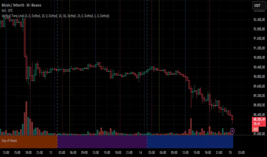
Vertical Time LinesVertical Time Lines is an indicator that draws vertical lines at specific times of each day on the price chart.
⚙️ Main Features
Up to 5 independent time lines
Precise hour and minute editing (HH:MM)
Individual enable/disable option per line
Customizable line color and style
Works on any asset and any timeframe
📝 Note
Due to Pine Script limitations, the lines are drawn using UTC time, not the time zone configured on the chart.
Lines are generated only when a candle exists exactly at the configured minute. If candles for the specified hours and minutes are not visible on the chart, the lines will not be displayed.
Time Liquidity a Zulu Kilo indicatorTime Liquidity (Daily/Weekly/Monthly/Quarterly/Yearly) — New York Time (ET)
Time Liquidity is a calendar-based “liquidity map” that tracks highs and lows for the current Day / Week / Month / Quarter / Year (using America/New_York time). When each period completes, its high/low becomes a persistent liquidity level that extends forward until price takes it—helping you quickly see where prior time-based liquidity is still “untouched.”
This is not a trading strategy and does not place trades. It is a context + levels tool designed to help you plan, frame targets, and monitor which higher-timeframe highs/lows remain in play.
What it plots:
1) Current period range boxes (optional)
-A live “bounding box” for the active D / W / M / Q / Y period, updating as new highs/lows form. This gives you better perspective
-Per-timeframe visibility controls and opacity controls.
2) Historical liquidity lines (optional)
-When a period rolls over, the completed period’s High (▲) and Low (▼) are projected forward as liquidity lines.
-Each line remains active until price breaches it (high taken when price trades above; low taken when price trades below).
-Tags identify the source timeframe (D/W/M/Q/Y) and side (high/low).
3) NeoHUD (optional)
-A compact panel showing the nearest next “untaken” liquidity above and below current price for each timeframe.
-Useful for quickly answering: “What’s the closest higher-timeframe high above me?” and “What’s the closest low below me?”
Time / session logic (important)
-All calendar boundaries are computed in New York time (America/New_York).
-Week start is Monday 00:00 ET.
-Sunday handling: you can choose whether Sunday merges into Monday (default behavior - This mostly for futures/FX markets) or is treated as a separate day (useful for Bitcoin, etc..).
(Note: This tool is calendar-based, not exchange-session-based. If your market has non-standard sessions/settlement conventions, interpret levels accordingly.)
How to use it (practical workflow)
-Turn on the timeframes you care about (D/W/M/Q/Y).
-Use current boxes to see the active period’s developing range.
-Use historical lines as a “to-do list” of still-untouched highs/lows.
-Watch the NeoHUD to stay oriented on the closest remaining liquidity above/below price (per timeframe).
For a cleaner chart or faster performance, reduce:
-Max Historical Liquidity Lines Kept / TF
-The number of enabled timeframes
-Glow/frame effects and/or boxes
Limitations / transparency
This indicator does not predict direction or guarantee outcomes; it only visualizes time-based highs/lows and whether they have been taken.
On very low timeframes or long histories, TradingView object limits may apply; use the settings above to manage chart load.
No alerts are included in this script (levels are intended for visual decision support).
Risk notice
Trading involves risk. This tool is provided for educational and informational purposes only and should not be used as the sole basis for trading decisions.

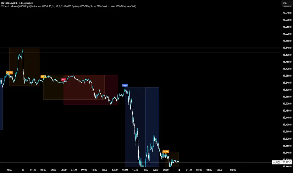
VX-Session-Boxes-(AM/PM Split)(Customizable) by Ikaru-s-VX-Session-Boxes-(AM/PM Split) is a session-based visualization tool for TradingView that highlights major market sessions directly on the chart using dotted range boxes and an optional AM/PM split.
The indicator allows traders to visually separate market behavior across different sessions while keeping the chart clean and readable.
🔹 Key Features
Custom Session Definitions
Define up to 4 independent sessions using TradingView’s session format (HHMM-HHMM + weekdays).
Timezone-Aware
All sessions are calculated using a user-defined timezone (IANA or UTC offset), ensuring accurate session alignment across markets.
Dotted Session Boxes
Each session is drawn as a dotted box based on the session’s high/low range, providing a clear view of volatility and price structure.
AM / PM Split Visualization
Sessions can be visually split into AM and PM parts:
Separate box shading for AM and PM
Optional dotted vertical split line at the AM → PM transition (12:00 in the selected timezone)
Session Labels
Optional labels at the start of each session for quick identification (e.g. Sydney, Tokyo, London, New York).
Fully Customizable Visuals
Adjustable opacity, border width, and visibility toggles for boxes, split lines, and labels.
🔹 Use Cases
Session-based market analysis (Asia / London / New York)
Identifying session ranges and volatility expansion
Observing price behavior differences between AM and PM
Studying session transitions and liquidity shifts
🔹 Notes
Session boxes are based on session high and low, not full chart height.
AM/PM split is based on 12:00 (noon) in the selected timezone.
Designed for clarity and performance on intraday timeframes.
🔹 Compatibility
Pine Script® v6
Works on all intraday timeframes
Overlay indicator (draws directly on the price chart)
CANDLE_TIME_RDThis tool displays the time of each candle directly on the chart by placing a label below
the bar with an upward-pointing arrow for clear visual alignment. It helps traders quickly
identify the exact timestamp of any candle during fast intraday analysis or historical review.
OVERVIEW
The script extracts the hour and minute of each bar, formats the timestamp according to the
user’s preference, and prints it beneath the candle. This removes the need to rely on the
data window or crosshair for time inspection. It is ideal for ITI evaluation, timestamp
journaling, and precise replay study.
FEATURES
- Prints the time under each candle or every N-th candle using a simple step input.
- Supports both AM/PM and military time through a toggle input.
- Builds all hour and minute text manually to ensure consistent formatting.
- Uses label.style_label_up to draw an arrow pointing toward the candle.
- Positions labels with yloc.belowbar so they do not overlap price bars.
USE CASES
- Reviewing setups with ChatGPT where exact candle timing matters.
- Studying EMA touches, VWAP interactions, or momentum shifts that occur at specific times.
- Journaling entries and exits with precise timestamps.
- Quickly identifying candle times without zooming or opening data windows.
This script is designed for clarity and convenience, improving workflow for structured
intraday traders and replay analysts.

Jerry's TrueDay Opening Ranges & H/L'sClick around. True Day H12 opening on Weekly and above, and H1 Attempted Direction Range on Daily.

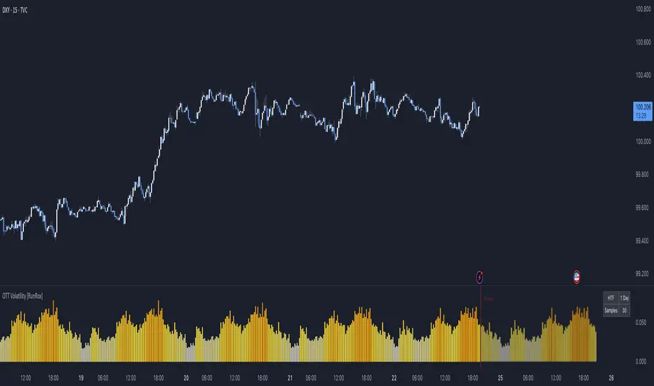
OTT Volatility [RunRox]📊 OTT Volatility is an indicator developed by the RunRox team to pinpoint the most optimal time to trade across different markets.
OTT stands for Optimal Trade Time Volatility and is designed primarily for markets without a fixed trading session, such as cryptocurrencies that trade 24/7. At the same time, it works equally well on any other market.
🔶 The concept is straightforward. The indicator takes a specified number of historical periods (Samples) and statistically evaluates which hours of the day or which days show the highest volatility for the selected asset.
As a result, it highlights time windows with elevated volatility where traders can focus on searching for trade setups and building positions.
🔶 As the core volatility metric, the indicator uses ATR (Average True Range) to measure intraday volatility. Then it calculates the average ATR value over the last N Samples, creating a statistically stable estimate of typical volatility for the selected asset.
🔶 Statistically, during these highlighted periods the market shows higher-than-average volatility.
This means that in these time windows price is more likely to be subject to stronger moves and potential manipulation, making them attractive for active trade execution and position management.
⚠️ However, historical behavior does not guarantee future results.
These periods should be treated only as zones where volatility has a higher probability of being above normal, not as a promise of movement.
As shown in the screenshot above, the indicator also projects potential future volatility based on historical data. This helps you better plan your trading hours and align your activity with periods where volatility is statistically expected to be higher or lower.
🔶 Current Volatility – as shown in the screenshot above, you can also monitor the real-time volatility of the market without any statistical averaging.
On top of that, you can overlay the current volatility on top of the statistical volatility levels, which makes it easy to see whether the market is now trading in a high- or low-volatility regime relative to its usual behavior.
4 display modes – you can choose any visualization style that fits your trading workflow:
Absolute – displays the raw volatility values.
Relative – shows volatility relative to its typical levels.
Average Centered – centers volatility around its average value.
Trim Low Value – filters out low-volatility noise and highlights only more significant moves.
This indicator helps you define the most effective trading hours on any market by relying on historical volatility statistics.
Use it to quickly see when your market tends to be more active and to structure your trading sessions around those periods.
✅ We hope this tool becomes a useful part of your trading toolkit and helps you improve the quality of your decisions and timing.
Trading Sessions [QuantAlgo]🟢 Overview
The Trading Sessions indicator tracks and displays the four major global trading sessions: Sydney, Tokyo, London, and New York. It provides session-based background highlighting, real-time price change tracking from session open, and a data table with session status. The script works across all markets (forex, equities, commodities, crypto) and helps traders identify when specific geographic markets are active, which directly correlates with changes in liquidity and volatility patterns. Default session times are set to major financial center hours in UTC but are fully adjustable to match your trading methodology.
🟢 Key Features
→ Session Background Color Coding
Each trading session gets a distinct background color on your chart:
1. Sydney Session - Default orange, 22:00-07:00 UTC
2. Tokyo Session - Default red, 00:00-09:00 UTC
3. London Session - Default green, 08:00-16:00 UTC
4. New York Session - Default blue, 13:00-22:00 UTC
When sessions overlap, the color priority is New York > London > Tokyo > Sydney. This means if London and New York are both active, the background shows New York's color. The priority matches typical liquidity and volatility patterns where later sessions generally show higher volume.
→ Color Customization
All session colors are configurable in the Color Settings panel:
1. Click any session color input to open the color picker
2. Select your preferred color for that session
3. Use the "Background Transparency" slider (0-100) to adjust opacity. Lower values = more visible, higher values = more subtle
4. Enable "Color Price Bars" to color candlesticks themselves according to the active session instead of just the background
The Color column in the info table shows a block (█) in each session's assigned color, matching what you see on the chart background.
→ Information Table Breakdown
→ Timeframe Warning
If you're viewing a timeframe of 12 hours or higher, a red warning label appears center-screen. Session boundaries don't render accurately on high timeframes because the time() function in Pine Script can't detect intra-bar session changes when each bar spans multiple sessions. The warning tells you to switch to sub-12H timeframes (e.g., 4H, 1H, 30m, 15m, etc.) for proper session detection. You can disable this warning in Color Settings if needed, but session highlighting can be unreliable on 12H+ charts regardless.
→ Time Range Configuration
Every session's time range is editable in Session Settings:
1. Click the time input field next to each session
2. Enter time as HHMM-HHMM in 24-hour format
3. All times are interpreted as UTC
4. Modify these to account for daylight saving shifts or to define custom session periods based on your backtested optimal trading windows
For example, if your strategy performs best during London/NY overlap specifically, you could set London to 08:00-17:00 and New York to 13:00-22:00 to ensure you see the full overlap highlighted.
→ Weekdays Filter
The "Weekdays Only (Mon-Fri)" toggle controls whether sessions display on weekends:
Enabled: Sessions only show Monday-Friday and hide on Saturday-Sunday. Use this for markets that close on weekends (most equities, forex).
Disabled: Sessions display 24/7 including weekends. Use this for markets that trade continuously (crypto).
→ Table Display Options
The info table has several configuration options in Table Settings:
Visibility: Toggle "Show Info Table" on/off to display or hide the entire table.
Position: Nine position options (Top/Middle/Bottom + Left/Center/Right) let you place the table wherever it doesn't block your price action or other indicators.
Text Size: Four size options (Tiny, Small, Normal, Large) to match your screen resolution and visual preferences.
→ Color Schemes:
Mono: Black background, gray header, white text
Light: White background, light gray header, black text
Blue: Dark blue background, medium blue header, white text
Custom: Manual selection of all five color components (table background, header background, header text, data text, borders)
→ Alert Functionality
The indicator includes ten alert conditions you can access via TradingView's alert system:
Session Opens:
1. Sydney Session Started
2. Tokyo Session Started
3. London Session Started
4. New York Session Started
5. Any Session Started
Session Closes:
6. Sydney Session Ended
7. Tokyo Session Ended
8. London Session Ended
9. New York Session Ended
10. Any Session Ended
These alerts fire when sessions transition based on your configured time ranges, letting you automate monitoring of session changes without watching the chart continuously. Useful for strategies that trade specific session opens/closes or need to adjust position sizing when volatility regime shifts between sessions.

Timed Swing Points [Free +] | cephxsTimed Swing Points | cephxs
This indicator is published under the Mozilla Public License 2.0. © cephxs, © fstarcapital
1. OVERVIEW
Timed Swing Points (TSP) highlights the timing of recent confirmed swing highs and lows and annotates them with context-aware time labels. Instead of drawing traditional pivot shapes and cluttering the chart, this streamlined free edition focuses on the temporal structure: WHEN pivots occur, not just WHERE . It helps discretionary traders quickly scan for clustering of swings around repeating intraday minutes or higher‑timeframe day names.
2. WHAT IT DOES
Detects swing highs and lows using a sensitivity factor (len)
Adds a time (or day name on daily timeframe) label at each qualified swing
Optional filtering to only show labels during defined "key time" minute windows
Automatically adapts label content to timeframe:
Intraday: HH:MM (24h or 12h model depending future input extension)
Daily: Full or abbreviated weekday names
Respects a maximum number of displayed swing points to keep charts clean
3. CORE FEATURES
Swing Detection: Uses ta.pivothigh(len, len) / ta.pivotlow(len, len); a pivot is confirmed only after enough bars pass, avoiding repaint on the current bar.
Time Labeling: Places labels offset back to the pivot bar index (bar_index - len).
Key Time Filtering: When enabled, labels only show if the pivot's minute is inside one of three windows: 00–10, 24–36, 50–59 minutes. These windows target common liquidity / volatility phases.
Day Name Mode: On daily timeframe, labels display full (e.g., Monday) or abbreviated (e.g., Mon) day names depending on the Full Day Names setting.
Point Limiting: Oldest labels are removed once Maximum Points Displayed is exceeded.
Clean Visual Footprint: Shape markers and lines are disabled in this free build (internally set to constants). Focus remains on time annotation density rather than price level persistence.
4. INPUTS & PARAMETERS
Sensitivity (len): Default 2. Swing pivot width. Higher = fewer, broader swings
Maximum Points Displayed: Default 10. Caps number of recent swing labels retained
Show Time Labels: Default true. Master toggle for all time labels
Key Times Only: Default true. Restricts labels to predefined minute windows
Prefix: Default blank. Optional text prepended to each label
High Time Color: Default red. Text color for swing high labels
Low Time Color: Default blue. Text color for swing low labels
Text Size: Default Small. Controls label text size (Tiny → Huge)
Full Day Names: Default true. Show full weekday names on daily timeframe
Internal Constants (Not User-Adjustable):
Shape display flags (show_high, show_low) set false
Line display and deletion logic present but disabled
Timezone currently fixed to America/New_York in Automatic mode; DST handled by TradingView engine
5. HOW SWING TIME IS DETERMINED
For each bar the script evaluates pivot conditions
A pivot is confirmed only after the right width (len) bars complete—the label is then placed len bars back
Time extraction uses the pivot's bar timestamp and converts:
Intraday: Formats HH:MM (24-hour). Infrastructure exists for future 12h toggle
Daily: Converts timestamp to a weekday name
Key time filter checks the pivot's minute bucket. If outside defined windows and filter is active, the label is skipped
6. TIME WINDOWS LOGIC (KEY TIMES ONLY)
Minutes 00–10 → Opening sequence & initial liquidity sweep
Minutes 24–36 → Post initial rotation / mid-hour inflection zone
Minutes 50–59 → Pre hour close / micro-structure reshuffle
ICT Traders: View as macros and note when macros form swing points
This pattern helps isolate intraday zones where structural shifts frequently occur, reducing noise from less consequential pivot timings.
7. USAGE GUIDELINES
Start with Sensitivity = 2 or 3 for most liquid intraday symbols. Increase on higher timeframes to avoid excessive clustering
Key Times Only ON: Ideal for focusing on session rotation pivots. OFF: Use for full discovery when studying custom time behaviors
Combine with volume profile or divergence tools to qualify time-labeled swings (e.g., a swing forming at 09:30 NY vs. random mid-bar)
Apply on lower timeframes (1–15m) to map recurring patterns or on Daily to see weekly rhythm changes
8. PERFORMANCE & LIMITATIONS
Efficient: Only stores arrays of recent labels and prunes aggressively
No Alerts: Current version does not fire alerts (Future Pro+ variant may include swing-time alerting)
Timezone: Fixed to America/New_York
9. BEST PRACTICES
Use a neutral chart theme; contrasting label colors amplify swing clusters
When analyzing historical pattern reliability, temporarily raise Maximum Points Displayed to 50–100 then revert to lighter values for live trading
Prefix field: Add a tag like "T:" if mixing multiple custom time tools to differentiate label origin
10. FAQ
Q: Why do some expected swings not show?
If they confirm outside key minute windows and filtering is ON, they're intentionally suppressed.
Q: Can I get price levels drawn?
Not in this free build. Lines/shapes are disabled intentionally.
Q: Does it repaint?
Pivot confirmation waits for the right width; labels appear only after the swing is locked in. Past labels aren't retroactively moved.
Q: Can I monitor multiple symbols at once?
This version is single‑symbol; use layouts or Pro variants for multi-source overlays.
11. CHANGELOG
v1.0 (Initial Free Release): Core swing time labeling, key time filter, day name adaptation, performance improvements. More updates coming.
12. DISCLAIMER
This tool is an analytical overlay designed for timing context only. It is NOT a standalone buy/sell signal. Always validate swings with broader market structure, liquidity pools, and risk management. No guarantee of future performance.
If you find this useful and want advanced variants (alerts, multi‑timezone, clustering metrics), reach out via TradingView. Feedback drives improvements.
