CandleTrack Pro | Pure Price Action Trend Detection CandleTrack Pro | Pure Price Action Trend Detection with Smart Candle Coloring
📝 Description:
CandleTrack Pro is a clean, lightweight trend-detection tool that uses only candle structure and ATR-based logic to determine market direction — no indicators, no overlays, just pure price action.
🔍 Features:
✅ Smart Candle-Based Trend Detection
Uses dynamic ATR thresholds to identify trend shifts with precision.
✅ Doji Protection Logic
Automatically filters indecision candles to avoid whipsaws and false signals.
✅ Dynamic Bull/Bear Color Coding
Bullish candles are colored green, bearish candles are colored red — see the trend instantly.
✅ No Noise, No Lag
No moving averages, no smoothing — just real-time decision-making power based on price itself.
📈 Ideal For:
Price action purists
Scalpers and intraday traders
Swing traders looking for clear visual bias
─────────────────────────────────────────────────────────────
Disclaimer:
This indicator is provided for educational and informational purposes only and should not be considered as financial or investment advice. The tool is designed to assist with technical analysis, but it does not guarantee any specific results or outcomes. All trading and investment decisions are made at your own risk. Past performance is not indicative of future results. Always do your own research and consult with a qualified financial advisor before making any trading decisions. The author accepts no liability for any losses or damages resulting from the use of this script. By using this indicator, you acknowledge and accept these terms.
─────────────────────────────────────────────────────────────
Sentiment

Ultra BUY SELL//@version=5
indicator("Ultra BUY SELL", overlay = false)
// Inputs
src = input(close, "Source", group = "Main settings")
p = input.int(180, "Trend period", group = "Main settings", tooltip = "Changes STRONG signals' sensitivity.", minval = 1)
atr_p = input.int(155, "ATR Period", group = "Main settings", minval = 1)
mult = input.float(2.1, "ATR Multiplier", step = 0.1, group = "Main settings", tooltip = "Changes sensitivity: higher period = higher sensitivty.")
mode = input.string("Type A", "Signal mode", options = , group = "Mode")
use_ema_smoother = input.string("No", "Smooth source with EMA?", options = , group = "Source")
src_ema_period = input(3, "EMA Smoother period", group = "Source")
color_bars = input(true, "Color bars?", group = "Addons")
signals_view = input.string("All", "Signals to show", options = , group = "Signal's Addon")
signals_shape = input.string("Labels", "Signal's shape", options = , group = "Signal's Addon")
buy_col = input(color.rgb(0, 255, 8), "Buy colour", group = "Signal's Addon", inline = "BS")
sell_col = input(color.rgb(255, 0, 0), "Sell colour", group = "Signal's Addon", inline = "BS")
// Calculations
src := use_ema_smoother == "Yes" ? ta.ema(src, src_ema_period) : src
// Source;
h = ta.highest(src, p)
// Highest of src p-bars back;
l = ta.lowest(src, p)
// Lowest of src p-bars back.
d = h - l
ls = ""
// Tracker of last signal
m = (h + l) / 2
// Initial trend line;
m := bar_index > p ? m : m
atr = ta.atr(atr_p)
// ATR;
epsilon = mult * atr
// Epsilon is a mathematical variable used in many different theorems in order to simplify work with mathematical object. Here it used as sensitivity measure.
change_up = (mode == "Type B" ? ta.cross(src, m + epsilon) : ta.crossover(src, m + epsilon)) or src > m + epsilon
// If price breaks trend line + epsilon (so called higher band), then it is time to update the value of a trend line;
change_down = (mode == "Type B" ? ta.cross(src, m - epsilon) : ta.crossunder(src, m - epsilon)) or src < m - epsilon
// If price breaks trend line - epsilon (so called higher band), then it is time to update the value of a trend line.
sb = open < l + d / 8 and open >= l
ss = open > h - d / 8 and open <= h
strong_buy = sb or sb or sb or sb or sb
strong_sell = ss or ss or ss or ss or ss
m := (change_up or change_down) and m != m ? m : change_up ? m + epsilon : change_down ? m - epsilon : nz(m , m)
// Updating the trend line.
ls := change_up ? "B" : change_down ? "S" : ls
// Last signal. Helps avoid multiple labels in a row with the same signal;
colour = ls == "B" ? buy_col : sell_col
// Colour of the trend line.
buy_shape = signals_shape == "Labels" ? shape.labelup : shape.triangleup
sell_shape = signals_shape == "Labels" ? shape.labeldown : shape.triangledown
// Plottings
// Signals with label shape
plotshape(signals_shape == "Labels" and (signals_view == "All" or signals_view == "Buy/Sell") and change_up and ls != "B" and not strong_buy, "Buy signal" , color = colour, style = buy_shape , location = location.belowbar, size = size.normal, text = "BUY", textcolor = color.white, force_overlay=true)
// Plotting the BUY signal;
plotshape(signals_shape == "Labels" and (signals_view == "All" or signals_view == "Buy/Sell") and change_down and ls != "S" and not strong_sell, "Sell signal" , color = colour, style = sell_shape, size = size.normal, text = "SELL", textcolor = color.white, force_overlay=true)
// Plotting the SELL signal.
plotshape(signals_shape == "Labels" and (signals_view == "All" or signals_view == "Strong") and change_up and ls != "B" and strong_buy, "Strong Buy signal" , color = colour, style = buy_shape , location = location.belowbar, size = size.normal, text = "STRONG", textcolor = color.white, force_overlay=true)
// Plotting the STRONG BUY signal;
plotshape(signals_shape == "Labels" and (signals_view == "All" or signals_view == "Strong") and change_down and ls != "S" and strong_sell, "Strong Sell signal" , color = colour, style = sell_shape, size = size.normal, text = "STRONG", textcolor = color.white, force_overlay=true)
// Plotting the STRONG SELL signal.
// Signal with arrow shape
plotshape(signals_shape == "Arrows" and (signals_view == "All" or signals_view == "Buy/Sell") and change_up and ls != "B" and not strong_buy, "Buy signal" , color = colour, style = buy_shape , location = location.belowbar, size = size.tiny, force_overlay=true)
// Plotting the BUY signal;
plotshape(signals_shape == "Arrows" and (signals_view == "All" or signals_view == "Buy/Sell") and change_down and ls != "S" and not strong_sell, "Sell signal" , color = colour, style = sell_shape, size = size.tiny, force_overlay=true)
// Plotting the SELL signal.
plotshape(signals_shape == "Arrows" and (signals_view == "All" or signals_view == "Strong") and change_up and ls != "B" and strong_buy, "Strong Buy signal" , color = colour, style = buy_shape , location = location.belowbar, size = size.tiny, force_overlay=true)
// Plotting the STRONG BUY signal;
plotshape(signals_shape == "Arrows" and (signals_view == "All" or signals_view == "Strong") and change_down and ls != "S" and strong_sell, "Strong Sell signal" , color = colour, style = sell_shape, size = size.tiny, force_overlay=true)
// Plotting the STRONG SELL signal.
barcolor(color_bars ? colour : na)
// Bar coloring
// Alerts
matype = input.string(title='MA Type', defval='EMA', options= )
ma_len1 = input(title='Short EMA1 Length', defval=5)
ma_len2 = input(title='Long EMA1 Length', defval=7)
ma_len3 = input(title='Short EMA2 Length', defval=5)
ma_len4 = input(title='Long EMA2 Length', defval=34)
ma_len5 = input(title='Short EMA3 Length', defval=98)
ma_len6 = input(title='Long EMA3 Length', defval=45)
ma_len7 = input(title='Short EMA4 Length', defval=7)
ma_len8 = input(title='Long EMA4 Length', defval=11)
ma_len9 = input(title='Short EMA5 Length', defval=11)
ma_len10 = input(title='Long EMA5 Length', defval=15)
ma_offset = input(title='Offset', defval=0)
//res = input(title="Resolution", type=resolution, defval="240")
f_ma(malen) =>
float result = 0
if matype == 'EMA'
result := ta.ema(src, malen)
result
if matype == 'SMA'
result := ta.sma(src, malen)
result
result
htf_ma1 = f_ma(ma_len1)
htf_ma2 = f_ma(ma_len2)
htf_ma3 = f_ma(ma_len3)
htf_ma4 = f_ma(ma_len4)
htf_ma5 = f_ma(ma_len5)
htf_ma6 = f_ma(ma_len6)
htf_ma7 = f_ma(ma_len7)
htf_ma8 = f_ma(ma_len8)
htf_ma9 = f_ma(ma_len9)
htf_ma10 = f_ma(ma_len10)
//plot(out1, color=green, offset=ma_offset)
//plot(out2, color=red, offset=ma_offset)
//lengthshort = input(8, minval = 1, title = "Short EMA Length")
//lengthlong = input(200, minval = 2, title = "Long EMA Length")
//emacloudleading = input(50, minval = 0, title = "Leading Period For EMA Cloud")
//src = input(hl2, title = "Source")
showlong = input(false, title='Show Long Alerts')
showshort = input(false, title='Show Short Alerts')
showLine = input(false, title='Display EMA Line')
ema1 = input(true, title='Show EMA Cloud-1')
ema2 = input(true, title='Show EMA Cloud-2')
ema3 = input(true, title='Show EMA Cloud-3')
ema4 = input(true, title='Show EMA Cloud-4')
ema5 = input(true, title='Show EMA Cloud-5')
emacloudleading = input.int(0, minval=0, title='Leading Period For EMA Cloud')
mashort1 = htf_ma1
malong1 = htf_ma2
mashort2 = htf_ma3
malong2 = htf_ma4
mashort3 = htf_ma5
malong3 = htf_ma6
mashort4 = htf_ma7
malong4 = htf_ma8
mashort5 = htf_ma9
malong5 = htf_ma10
cloudcolour1 = mashort1 >= malong1 ? color.rgb(0, 255, 0) : color.rgb(255, 0, 0)
cloudcolour2 = mashort2 >= malong2 ? #4caf4f47 : #ff110047
cloudcolour4 = mashort4 >= malong4 ? #4caf4f52 : #f2364652
cloudcolour5 = mashort5 >= malong5 ? #33ff0026 : #ff000026
//03abc1
mashortcolor1 = mashort1 >= mashort1 ? color.olive : color.maroon
mashortcolor2 = mashort2 >= mashort2 ? color.olive : color.maroon
mashortcolor3 = mashort3 >= mashort3 ? color.olive : color.maroon
mashortcolor4 = mashort4 >= mashort4 ? color.olive : color.maroon
mashortcolor5 = mashort5 >= mashort5 ? color.olive : color.maroon
mashortline1 = plot(ema1 ? mashort1 : na, color=showLine ? mashortcolor1 : na, linewidth=1, offset=emacloudleading, title='Short Leading EMA1', force_overlay=true)
mashortline2 = plot(ema2 ? mashort2 : na, color=showLine ? mashortcolor2 : na, linewidth=1, offset=emacloudleading, title='Short Leading EMA2', force_overlay=true)
mashortline3 = plot(ema3 ? mashort3 : na, color=showLine ? mashortcolor3 : na, linewidth=1, offset=emacloudleading, title='Short Leading EMA3', force_overlay=true)
mashortline4 = plot(ema4 ? mashort4 : na, color=showLine ? mashortcolor4 : na, linewidth=1, offset=emacloudleading, title='Short Leading EMA4', force_overlay=true)
mashortline5 = plot(ema5 ? mashort5 : na, color=showLine ? mashortcolor5 : na, linewidth=1, offset=emacloudleading, title='Short Leading EMA5', force_overlay=true)
malongcolor1 = malong1 >= malong1 ? color.green : color.red
malongcolor2 = malong2 >= malong2 ? color.green : color.red
malongcolor3 = malong3 >= malong3 ? color.green : color.red
malongcolor4 = malong4 >= malong4 ? color.green : color.red
malongcolor5 = malong5 >= malong5 ? color.green : color.red
malongline1 = plot(ema1 ? malong1 : na, color=showLine ? malongcolor1 : na, linewidth=3, offset=emacloudleading, title='Long Leading EMA1', force_overlay=true)
malongline2 = plot(ema2 ? malong2 : na, color=showLine ? malongcolor2 : na, linewidth=3, offset=emacloudleading, title='Long Leading EMA2', force_overlay=true)
malongline3 = plot(ema3 ? malong3 : na, color=showLine ? malongcolor3 : na, linewidth=3, offset=emacloudleading, title='Long Leading EMA3', force_overlay=true)
malongline4 = plot(ema4 ? malong4 : na, color=showLine ? malongcolor4 : na, linewidth=3, offset=emacloudleading, title='Long Leading EMA4', force_overlay=true)
malongline5 = plot(ema5 ? malong5 : na, color=showLine ? malongcolor5 : na, linewidth=3, offset=emacloudleading, title='Long Leading EMA5', force_overlay=true)
fill(mashortline1, malongline1, color=cloudcolour1, title='MA Cloud1', transp=45)
fill(mashortline2, malongline2, color=cloudcolour2, title='MA Cloud2', transp=65)
fill(mashortline4, malongline4, color=cloudcolour4, title='MA Cloud4', transp=65)
fill(mashortline5, malongline5, color=cloudcolour5, title='MA Cloud5', transp=65)
leftBars = input(15, title='Left Bars ')
rightBars = input(15, title='Right Bars')
volumeThresh = input(20, title='Volume Threshold')
//
highUsePivot = fixnan(ta.pivothigh(leftBars, rightBars) )
lowUsePivot = fixnan(ta.pivotlow(leftBars, rightBars) )
r1 = plot(highUsePivot, color=ta.change(highUsePivot) ? na : #FF0000, linewidth=3, offset=-(rightBars + 1), title='Resistance', force_overlay=true)
s1 = plot(lowUsePivot, color=ta.change(lowUsePivot) ? na : #00ff0d, linewidth=3, offset=-(rightBars + 1), title='Support', force_overlay=true)
//Volume %
short = ta.ema(volume, 5)
long = ta.ema(volume, 10)
osc = 100 * (short - long) / long
//For bull / bear wicks
// This Pine Script™ code is subject to the terms of the Mozilla Public License 2.0 at mozilla.org
// © divudivu600
// Developer By ALCON ALGO
//telegram : @harmonicryptosignals
//@version = 5
//indicator(shorttitle='Oscillator Vision', title='Alcon Oscillator Vision', overlay=false)
n1 = input(10, 'Channel length')
n2 = input(21, 'Average length')
reaction_wt = input.int(defval=1, title='Reaction in change of direction', minval=1)
nsc = input.float(53, 'Levels About Buys', minval=0.0)
nsv = input.float(-53, 'Levels About Sells', maxval=-0.0)
Buy_sales = input(true, title='Only Smart Buy Reversal')
Sell_sales = input(true, title='Only Smart Sell Reversal')
Histogram = input(true, title='Show Histogarm')
//Trendx = input(false, title='Show Trendx')
barras = input(true, title='Divergence on chart(Bars)')
divregbull = input(true, title='Regular Divergence Bullish')
divregbear = input(true, title='Regular Divergence Bearish')
divhidbull = input(true, title='Show Divergence Hidden Bullish')
divhidbear = input(true, title='Show Divergence Hidden Bearish')
Tags = input(true, title='Show Divergence Lable')
amme = input(false, title='Activar media movil Extra para WT')
White = #FDFEFE
Black = #000000
Bearish = #e91e62
Bullish = #18e0ff
Strong_Bullish = #2962ff
Bullish2 = #00bedc
Blue1 = #00D4FF
Blue2 = #009BBA
orange = #FF8B00
yellow = #FFFB00
LEZ = #0066FF
purp = #FF33CC
// Colouring
tf(_res, _exp, gaps_on) =>
gaps_on == 0 ? request.security(syminfo.tickerid, _res, _exp) : gaps_on == true ? request.security(syminfo.tickerid, _res, _exp, barmerge.gaps_on, barmerge.lookahead_off) : request.security(syminfo.tickerid, _res, _exp, barmerge.gaps_off, barmerge.lookahead_off)
ha_htf = ''
show_ha = input.bool(true, "Show HA Plot/ Market Bias", group="HA Market Bias")
ha_len = input(7, 'Period', group="HA Market Bias")
ha_len2 = input(10, 'Smoothing', group="HA Market Bias")
// Calculations {
o = ta.ema(open, ha_len)
c = ta.ema(close, ha_len)
h1 = ta.ema(high, ha_len)
l1 = ta.ema(low, ha_len)
haclose = tf(ha_htf, (o + h1 + l1 + c) / 4, 0)
xhaopen = tf(ha_htf, (o + c) / 2, 0)
haopen = na(xhaopen ) ? (o + c) / 2 : (xhaopen + haclose ) / 2
hahigh = math.max(h1, math.max(haopen, haclose))
halow = math.min(l1, math.min(haopen, haclose))
o2 = tf(ha_htf, ta.ema(haopen, ha_len2), 0)
c2 = tf(ha_htf, ta.ema(haclose, ha_len2), 0)
h2 = tf(ha_htf, ta.ema(hahigh, ha_len2), 0)
l2 = tf(ha_htf, ta.ema(halow, ha_len2), 0)
ha_avg = (h2 + l2) / 2
// }
osc_len = 8
osc_bias = 100 *(c2 - o2)
osc_smooth = ta.ema(osc_bias, osc_len)
sigcolor =
(osc_bias > 0) and (osc_bias >= osc_smooth) ? color.new(Bullish, 35) :
(osc_bias > 0) and (osc_bias < osc_smooth) ? color.new(Bullish2, 75) :
(osc_bias < 0) and (osc_bias <= osc_smooth) ? color.new(Bearish, 35) :
(osc_bias < 0) and (osc_bias > osc_smooth) ? color.new(Bearish, 75) :
na
// }
nsc1 = nsc
nsc2 = nsc + 5
nsc3 = nsc + 10
nsc4 = nsc + 15
nsc5 = nsc + 20
nsc6 = nsc + 25
nsc7 = nsc + 30
nsc8 = nsc + 35
nsv1 = nsv - 5
nsv2 = nsv - 10
nsv3 = nsv - 15
nsv4 = nsv - 20
nsv5 = nsv - 25
nsv6 = nsv - 30
nsv7 = nsv - 35
nsv8 = nsv - 40
ap = hlc3
esa = ta.ema(ap, n1)
di = ta.ema(math.abs(ap - esa), n1)
ci = (ap - esa) / (0.015 * di)
tci = ta.ema(ci, n2)
wt1 = tci
wt2 = ta.sma(wt1, 4)
direction = 0
direction := ta.rising(wt1, reaction_wt) ? 1 : ta.falling(wt1, reaction_wt) ? -1 : nz(direction )
Change_of_direction = ta.change(direction, 1)
pcol = direction > 0 ? Strong_Bullish : direction < 0 ? Bearish : na
obLevel1 = input(60, 'Over Bought Level 1')
obLevel2 = input(53, 'Over Bought Level 2')
osLevel1 = input(-60, 'Over Sold Level 1')
osLevel2 = input(-53, 'Over Sold Level 2')
rsi = ta.rsi(close,14)
color greengrad = color.from_gradient(rsi, 10, 90, #00ddff, #007d91)
color redgrad = color.from_gradient(rsi, 10, 90, #8b002e, #e91e62)
ob1 = plot(obLevel1, color=#e91e6301)
os1 = plot(osLevel1, color=#00dbff01)
ob2 = plot(obLevel2, color=#e91e6301)
os2 = plot(osLevel2, color=#00dbff01)
p1 = plot(wt1, color=#00dbff01)
p2 = plot(wt2, color=#e91e6301)
plot(wt1 - wt2, color=wt2 - wt1 > 0 ? redgrad : greengrad, style=plot.style_columns)
// fill(p1,p2,color = wt2 - wt1 > 0 ? redgrad: greengrad) // old
fill(p1,p2,color = sigcolor)
// new
fill(ob1,ob2,color = #e91e6350)
fill(os1,os2,color = #00dbff50)
midpoint = (nsc + nsv) / 2
ploff = (nsc - midpoint) / 8
BullSale = ta.crossunder(wt1, wt2) and wt1 >= nsc and Buy_sales == true
BearSale = ta.crossunder(wt1, wt2) and Buy_sales == false
Bullishh = ta.crossover(wt1, wt2) and wt1 <= nsv and Sell_sales == true
Bearishh = ta.crossover(wt1, wt2) and Sell_sales == false
plot(BullSale ? wt2 + ploff : na, style=plot.style_circles, color=color.new(Bearish, 0), linewidth=6, title='BuysG')
plot(BearSale ? wt2 + ploff : na, style=plot.style_circles, color=color.new(Bearish, 0), linewidth=6, title='SellsG')
plot(Bullishh ? wt2 - ploff : na, style=plot.style_circles, color=color.new(Strong_Bullish, 0), linewidth=6, title='Buys On Sale')
plot(Bearishh ? wt2 - ploff : na, style=plot.style_circles, color=color.new(Strong_Bullish, 0), linewidth=6, title='Sells on Sale')
//plot(Histogram ? wt1 - wt2 : na, style=plot.style_area, color=color.new(Blue2, 80), linewidth=1, title='Histograma')
//barcolor(barras == true and Bullishh == true or barras == true and Bearishh == true ? Bullish2 : na)
//barcolor(barras == true and BullSale == true or barras == true and BearSale == true ? Bearish : na)
/////// Divergence ///////
f_top_fractal(_src) =>
_src < _src and _src < _src and _src > _src and _src > _src
f_bot_fractal(_src) =>
_src > _src and _src > _src and _src < _src and _src < _src
f_fractalize(_src) =>
f_top_fractal(_src) ? 1 : f_bot_fractal(_src) ? -1 : 0
fractal_top1 = f_fractalize(wt1) > 0 ? wt1 : na
fractal_bot1 = f_fractalize(wt1) < 0 ? wt1 : na
high_prev1 = ta.valuewhen(fractal_top1, wt1 , 0)
high_price1 = ta.valuewhen(fractal_top1, high , 0)
low_prev1 = ta.valuewhen(fractal_bot1, wt1 , 0)
low_price1 = ta.valuewhen(fractal_bot1, low , 0)
regular_bearish_div1 = fractal_top1 and high > high_price1 and wt1 < high_prev1 and divregbear == true
hidden_bearish_div1 = fractal_top1 and high < high_price1 and wt1 > high_prev1 and divhidbear == true
regular_bullish_div1 = fractal_bot1 and low < low_price1 and wt1 > low_prev1 and divregbull == true
hidden_bullish_div1 = fractal_bot1 and low > low_price1 and wt1 < low_prev1 and divhidbull == true
col1 = regular_bearish_div1 ? Bearish : hidden_bearish_div1 ? Bearish : na
col2 = regular_bullish_div1 ? Strong_Bullish : hidden_bullish_div1 ? Strong_Bullish : na
//plot(title='Divergence Bearish', series=fractal_top1 ? wt1 : na, color=col1, linewidth=2, transp=0)
//plot(title='Divergence Bullish', series=fractal_bot1 ? wt1 : na, color=col2, linewidth=2, transp=0)
plotshape(regular_bearish_div1 and divregbear and Tags ? wt1 + ploff * 1 : na, title='Divergence Regular Bearish', text='Bear', location=location.absolute, style=shape.labeldown, size=size.tiny, color=color.new(Bearish, 0), textcolor=color.new(White, 0))
plotshape(hidden_bearish_div1 and divhidbear and Tags ? wt1 + ploff * 1 : na, title='Divergence Hidden Bearish', text='H Bear', location=location.absolute, style=shape.labeldown, size=size.tiny, color=color.new(Bearish, 0), textcolor=color.new(White, 0))
plotshape(regular_bullish_div1 and divregbull and Tags ? wt1 - ploff * 1 : na, title='Divergence Regular Bullish', text='Bull', location=location.absolute, style=shape.labelup, size=size.tiny, color=color.new(Strong_Bullish, 0), textcolor=color.new(White, 0))
plotshape(hidden_bullish_div1 and divhidbull and Tags ? wt1 - ploff * 1 : na, title='Divergence Hidden Bullish', text='H Bull', location=location.absolute, style=shape.labelup, size=size.tiny, color=color.new(Strong_Bullish, 0), textcolor=color.new(White, 0))
/////// Unfazed Alerts //////
////////////////////////////////////////////////-MISTERMOTA MOMENTUM-/////////////////////////////////////
source = input(close)
responsiveness = math.max(0.00001, input.float(0.9, minval=0.0, maxval=1.0))
periodd = input(50)
sd = ta.stdev(source, 50) * responsiveness
var worm = source
diff = source - worm
delta = math.abs(diff) > sd ? math.sign(diff) * sd : diff
worm += delta
ma = ta.sma(source, periodd)
raw_momentum = (worm - ma) / worm
current_med = raw_momentum
min_med = ta.lowest(current_med, periodd)
max_med = ta.highest(current_med, periodd)
temp = (current_med - min_med) / (max_med - min_med)
value = 0.5 * 2
value *= (temp - .5 + .5 * nz(value ))
value := value > .9999 ? .9999 : value
value := value < -0.9999 ? -0.9999 : value
temp2 = (1 + value) / (1 - value)
momentum = .25 * math.log(temp2)
momentum += .5 * nz(momentum )
//momentum := raw_momentum
signal = nz(momentum )
trend = math.abs(momentum) <= math.abs(momentum )
////////////////////////////////////////////////-GROWING/FAILING-//////////////////////////////////////////
length = input.int(title="MOM Period", minval=1, defval=14, group="MOM Settings")
srcc = input(title="MOM Source", defval=hlc3, group="MOM Settings")
txtcol_grow_above = input(#1a7b24, "Above Grow", group="MOM Settings", inline="Above")
txtcol_fall_above = input(#672ec5, "Fall", group="MOM Settings", inline="Above")
txtcol_grow_below = input(#F37121, "Below Grow", group="MOM Settings", inline="Below")
txtcol_fall_below = input(#be0606, "Fall", group="MOM Settings", inline="Below")
ma(source, length, type) =>
switch type
"SMA" => ta.sma(source, length)
"EMA" => ta.ema(source, length)
"SMMA (RMA)" => ta.rma(source, length)
"WMA" => ta.wma(source, length)
"VWMA" => ta.vwma(source, length)
typeMA = input.string(title = "Method", defval = "SMA", options= , group="MA Settings")
smoothingLength = input.int(title = "Length", defval = 5, minval = 1, maxval = 100, group="MA Settings")
smoothingLine = ma(delta, smoothingLength, typeMA)
deltaText=(delta > 0 ? (delta > delta ? " MOM > 0 and ▲ Growing, MOM = " + str.tostring(delta , "#.##") :" MOM > 0 and ▼ Falling, MOM = " + str.tostring(delta , "#.##") ) : (delta > delta ? "MOM < 0 and ▲ Growing, MOM = " + str.tostring(delta , "#.##"): " MOM < 0 and ▼ Falling, MOM = " + str.tostring(delta , "#.##")))
oneDay = 24 * 60 * 60 * 1000
barsAhead = 3
tmf = if timeframe.ismonthly
barsAhead * oneDay * 30
else if timeframe.isweekly
barsAhead * oneDay * 7
else if timeframe.isdaily
barsAhead * oneDay
else if timeframe.isminutes
barsAhead * oneDay * timeframe.multiplier / 1440
else if timeframe.isseconds
barsAhead * oneDay * timeframe.multiplier / 86400
else
0
angle(_src) =>
rad2degree = 180 / 3.14159265359
//pi
ang = rad2degree * math.atan((_src - _src ) / ta.atr(14))
ang
emae = angle(smoothingLine)
emaanglestat = emae > emae ? "▲ Growing": "▼ Falling"
deltaTextxxx = "MOM MA/ATR angle value is " + str.tostring(emae, "#.##") + "° and is " + emaanglestat
deltacolorxxx = emae >0 and emae >=emae ? txtcol_grow_above : txtcol_fall_below
// Label
label lpt1 = label.new(time, -30, text=deltaTextxxx , color=deltacolorxxx, xloc=xloc.bar_time, style=label.style_label_left, textcolor=color.white, textalign=text.align_left, size=size.normal)
label.set_x(lpt1, label.get_x(lpt1) + tmf)
label.delete(lpt1 )
txtdeltaColors = (delta > 50 ? (delta < delta ? txtcol_grow_above : txtcol_fall_above) : (delta < delta ? txtcol_grow_below : txtcol_fall_below))
label ldelta1 = label.new(time, 30, text=deltaText , color=txtdeltaColors, xloc=xloc.bar_time, style=label.style_label_left, textcolor=color.white, textalign=text.align_left, size=size.normal)
label.set_x(ldelta1, label.get_x(ldelta1) + tmf)
label.delete(ldelta1 )

Tension Squeeze Clock v1.0🔥 Tension Squeeze Clock v1.0
Forecast explosive market moves before they happen.
The Tension Squeeze Clock is a cyclical compression detector that identifies when the market is storing energy across multiple dimensions — and signals when that energy is about to uncoil.
This indicator combines three critical components:
🔹 RSI Contraction – Detects when momentum is balanced and compressed
🔹 Volatility Squeeze – Measures low standard deviation in price movement
🔹 Range Tension – Flags tight candle ranges relative to average volatility
When all three compressions align, the indicator prints a clear “Squeeze Ready” signal. When the pressure breaks, it signals “Squeeze Uncoiling” — a prime moment to watch for volatility surges or directional breakouts.
📈 Recommended Usage
🔍 This tool works especially well on the Daily timeframe, where coiled conditions often lead to significant price expansions.
Use it to:
Anticipate breakout setups
Confirm coiled consolidation zones
Add timing precision to your volume or divergence-based strategies
📊 Display Options
Panel view with bar colors to reflect compression strength
On-chart labels for squeeze signals
Optional alerts when a squeeze begins or breaks
Whether you're swing trading, trend riding, or timing reversals, the Tension Squeeze Clock helps you see what most indicators miss: the calm before the storm.

RSI with 2-Pole FilterA momentum indicator that tells you if a stock is overbought or oversold.
RSI goes between 0 and 100.
70 = overbought (might fall)
<30 = oversold (might rise)
It often looks jagged or choppy on volatile days.
Think of this filter like a momentum smoother:
It still follows RSI closely,
But it doesn’t react to every little jiggle in price,
Which helps avoid false signals.
it keeps track of:
The current RSI,
The last 2 RSI values (inputs), and
The last 2 outputs (filtered RSIs).
It uses feedback to shape the output based on previous values, making it smoother than a simple moving average.

Top Crypto Above 28-Day AverageDescription
The “Top Crypto Above 28-Day Average” (CRYPTOTW) script scans a selectable universe of up to 120 top-capitalization cryptocurrencies (divided into customizable 40-symbol batches), then plots the count of those trading above their own 28-period simple moving average. It helps you gauge broad market strength and identify which tokens are showing momentum relative to their recent trend.
Key Features
• Batch Selection: Choose among “Top40,” “Mid40,” or “Low40” market-cap groups, or set a custom batch size (up to 40 symbols) to keep within the API limit.
• Dynamic Plot: Displays a live line chart of how many cryptos are above their 28-day MA on each bar.
• Reference Lines: Automatic horizontal lines at 25%, 50%, and 75% of your batch to provide quick visual thresholds.
• Background Coloration: The chart background shifts green/yellow/red based on whether more than 70%, 50–70%, or under 50% of the batch is above the MA.
• Optional Table: On the final bar, show a sortable table of up to 28 tickers currently above their 28-day MA, including current price, percent above MA, and “Above” status color-coding.
• Alerts:
• Strong Batch Performance: Fires when >70% of the batch is above the MA.
• Weak Batch Performance: Fires when <10 cryptos (i.e. <25%) are above the MA.
Inputs
• Show Results Table (show_table): Toggle the detailed table on/off.
• Table Position (table_position): Select one of the four corners for your table overlay.
• Max Cryptos to Display (max_display): Limit the number of rows in the results table.
• Current Batch (current_batch): Pick “Top40,” “Mid40,” or “Low40.”
• Batch Size (batch_size): Define the number of symbols (1–40) you want to include from the chosen batch.
How to Use
1. Add the CRYPTOTW indicator to any chart.
2. Select your batch and size to focus on the segment of the crypto market you follow.
3. Watch the plotted line to see the proportion of tokens with bullish momentum.
4. (Optional) Enable the results table to see exactly which tokens are outperforming their 28-day average.
5. Set alerts to be notified when the batch either overheats (strong performance) or cools off significantly.
Why It Matters
By tracking the share of assets riding their 28-day trend, you gain a macro-level view of market breadth—crucial for spotting emerging rallies or early signs of broad weakness. Whether you’re swing-trading individual altcoins or assessing overall market mood, this tool distills complex data into an intuitive, actionable signal.

market rsi vs chart rsi🔍 Key Features:
- Aggregate RSI Sentiment: Measures average momentum across major crypto assets including BTC, ETH, SOL, and others.
- Custom Weighting Options: Choose between equal weighting, volume-based, or market cap-based influence.
- Dual RSI Display:
- Chart RSI: Line plot with color-coded overbought/oversold zones.
- Market RSI: Circular markers for added clarity.
- Dynamic Background Alerts: Highlights periods of collective bullish or bearish pressure.
🎯 Use Cases:
- Spot market-wide divergences.
- Detect chart-specific outliers in momentum.
- Improve decision-making for entries and exits by overlaying local RSI against macro signals.
Not financial advice. Only for crypto trading.

SNIPERKILLS NQ JULY 18 2025, GAMEPLANNQ GAME PLAN JULY 18, 2025!
✅ Bullish Scenario
Condition: Price breaks and holds above 23,279.75
Targets:
🎯 Target 1: 23,320 — minor imbalance / reaction zone
🎯 Target 2: 23,375 — potential liquidity sweep
🎯 Target 3: 23,420 — psychological level / extended move
Stop Loss: Below 23,234.25 (Short Trigger / invalidation)
❌ Bearish Scenario
Condition: Price breaks and holds below 23,234.25
Targets:
🎯 Target 1: 23,200 — FVG or intraday demand
🎯 Target 2: 23,150 — mid-range flush target
🎯 Target 3: 23,017 — prior day’s low & major liquidity zone
Stop Loss: Above 23,279.75 (Long Trigger / invalidation)


Kyber Cell's – TTM Squeeze Pro
Kyber Cell's TTM Squeeze Pro is an all-in-one overlay that rebuilds John Carter’s TTM Squeeze, then layers on two extra confirmation tools—ALMA trend and a scroll-aware VWAP—so you can track contraction, momentum, trend and value without stacking indicators.
⸻
What each visual means
• Candles = Momentum histogram
Instead of a separate lower pane, every bar is tinted by a linear-regression slope:
• Rising & above zero → aqua→blue (bullish strength)
• Falling & below zero → yellow→red (bearish strength)
• Dots above the bars = Squeeze status
I’ve modernized Carter’s original black→red→orange→green sequence (it didn't feel natural to me):
• Blue “Cool” – bands wide apart, no compression yet
• Orange “Warming” – loose compression building
• Red “Ready” – tightest compression, watch for release
• Green “GO!” – first bar the squeeze fires (breakout begins)
• I added a Red/Green Backdrop that tracks the squeeze so you can easily identify the entry and exit based on the squeeze momentum. Appears only after a squeeze fires. Stays green while momentum remains > 0, red while it is < 0. Clears when momentum flips or a new squeeze starts.
• ALMA ribbon
A 50-period Arnaud Legoux moving average (user-tunable).
Price and ribbon rising above it → bullish tilt; price under a falling ribbon → bearish tilt.
• VWAP with optional σ bands
Anchored to the left-most visible bar every time you pan/zoom, so it always reflects the range on your screen. Staying above VWAP supports longs; below supports shorts.
• Entry labels
A triangle ▲/▼ or arrow ↑/↓ (your choice) prints on the exact bar a squeeze fires. Color, size and ATR padding are adjustable.
Key inputs you can adjust
• Squeeze length, Bollinger σ, three Keltner multipliers (High/Mid/Low).
• ALMA length, offset (0 = fast, 1 = smooth) and sigma.
• VWAP on/off, deviation-band σ (set to 0 to hide bands).
• Marker shape, size, colours and vertical padding in ATR multiples.
Typical workflow
1. Watch dot color: blue → orange → red.
2. When the dot flips green, momentum bar confirms aqua/blue (bull) or yellow/red (bear).
3. Enter in the direction of the bar color if price is also on the supportive side of ALMA and/or VWAP.
4. Trail until momentum changes side, the backdrop disappears, or your target is hit.
Disclaimer — This script is for educational purposes only and is not financial advice. Test thoroughly and manage risk before live trading.

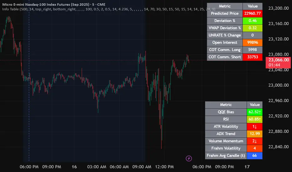
Info TableOverview
The Info Table V1 is a versatile TradingView indicator tailored for intraday futures traders, particularly those focusing on MESM2 (Micro E-mini S&P 500 futures) on 1-minute charts. It presents essential market insights through two customizable tables: the Main Table for predictive and macro metrics, and the New Metrics Table for momentum and volatility indicators. Designed for high-activity sessions like 9:30 AM–11:00 AM CDT, this tool helps traders assess price alignment, sentiment, and risk in real-time. Metrics update dynamically (except weekly COT data), with optional alerts for key conditions like volatility spikes or momentum shifts.
This indicator builds on foundational concepts like linear regression for predictions and adapts open-source elements for enhanced functionality. Gradient code is adapted from TradingView's Color Library. QQE logic is adapted from LuxAlgo's QQE Weighted Oscillator, licensed under CC BY-NC-SA 4.0. The script is released under the Mozilla Public License 2.0.
Key Features
Two Customizable Tables: Positioned independently (e.g., top-right for Main, bottom-right for New Metrics) with toggle options to show/hide for a clutter-free chart.
Gradient Coloring: User-defined high/low colors (default green/red) for quick visual interpretation of extremes, such as overbought/oversold or high volatility.
Arrows for Directional Bias: In the New Metrics Table, up (↑) or down (↓) arrows appear in value cells based on metric thresholds (top/bottom 25% of range), indicating bullish/high or bearish/low conditions.
Consensus Highlighting: The New Metrics Table's title cells ("Metric" and "Value") turn green if all arrows are ↑ (strong bullish consensus), red if all are ↓ (strong bearish consensus), or gray otherwise.
Predicted Price Plot: Optional line (default blue) overlaying the ML-predicted price for visual comparison with actual price action.
Alerts: Notifications for high/low Frahm Volatility (≥8 or ≤3) and QQE Bias crosses (bullish/bearish momentum shifts).
Main Table Metrics
This table focuses on predictive, positional, and macro insights:
ML-Predicted Price: A linear regression forecast using normalized price, volume, and RSI over a customizable lookback (default 500 bars). Gradient scales from low (red) to high (green) relative to the current price ± threshold (default 100 points).
Deviation %: Percentage difference between current price and predicted price. Gradient highlights extremes (±0.5% default threshold), signaling potential overextensions.
VWAP Deviation %: Percentage difference from Volume Weighted Average Price (VWAP). Gradient indicates if price is above (green) or below (red) fair value (±0.5% default).
FRED UNRATE % Change: Percentage change in U.S. unemployment rate (via FRED data). Cell turns red for increases (economic weakness), green for decreases (strength), gray if zero or disabled.
Open Interest: Total open MESM2 futures contracts. Gradient scales from low (red) to high (green) up to a hardcoded 300,000 threshold, reflecting market participation.
COT Commercial Long/Short: Weekly Commitment of Traders data for commercial positions. Long cell green if longs > shorts (bullish institutional sentiment); Short cell red if shorts > longs (bearish); gray otherwise.
New Metrics Table Metrics
This table emphasizes technical momentum and volatility, with arrows for quick bias assessment:
QQE Bias: Smoothed RSI vs. trailing stop (default length 14, factor 4.236, smooth 5). Green for bullish (RSI > stop, ↑ arrow), red for bearish (RSI < stop, ↓ arrow), gray for neutral.
RSI: Relative Strength Index (default period 14). Gradient from oversold (red, <30 + threshold offset, ↓ arrow if ≤40) to overbought (green, >70 - offset, ↑ arrow if ≥60).
ATR Volatility: Score (1–20) based on Average True Range (default period 14, lookback 50). High scores (green, ↑ if ≥15) signal swings; low (red, ↓ if ≤5) indicate calm.
ADX Trend: Average Directional Index (default period 14). Gradient from weak (red, ↓ if ≤0.25×25 threshold) to strong trends (green, ↑ if ≥0.75×25).
Volume Momentum: Score (1–20) comparing current to historical volume (lookback 50). High (green, ↑ if ≥15) suggests pressure; low (red, ↓ if ≤5) implies weakness.
Frahm Volatility: Score (1–20) from true range over a window (default 24 hours, multiplier 9). Dynamic gradient (green/red/yellow); ↑ if ≥7.5, ↓ if ≤2.5.
Frahm Avg Candle (Ticks): Average candle size in ticks over the window. Blue gradient (or dynamic green/red/yellow); ↑ if ≥0.75 percentile, ↓ if ≤0.25.
Arrows trigger on metric-specific logic (e.g., RSI ≥60 for ↑), providing directional cues without strict color ties.
Customization Options
Adapt the indicator to your strategy:
ML Inputs: Lookback (10–5000 bars) and RSI period (2+) for prediction sensitivity—shorter for volatility, longer for trends.
Timeframes: Individual per metric (e.g., 1H for QQE Bias to match higher frames; blank for chart timeframe).
Thresholds: Adjust gradients and arrows (e.g., Deviation 0.1–5%, ADX 0–100, RSI overbought/oversold).
QQE Settings: Length, factor, and smooth for fine-tuned momentum.
Data Toggles: Enable/disable FRED, Open Interest, COT for focus (e.g., disable macro for pure intraday).
Frahm Options: Window hours (1+), scale multiplier (1–10), dynamic colors for avg candle.
Plot/Table: Line color, positions, gradients, and visibility.
Ideal Use Case
Perfect for MESM2 scalpers and trend traders. Use the Main Table for entry confirmation via predicted deviations and institutional positioning. Leverage the New Metrics Table arrows for short-term signals—enter bullish on green consensus (all ↑), avoid chop on low volatility. Set alerts to catch shifts without constant monitoring.
Why It's Valuable
Info Table V1 consolidates diverse metrics into actionable visuals, answering critical questions: Is price mispriced? Is momentum aligning? Is volatility manageable? With real-time updates, consensus highlights, and extensive customization, it enhances precision in fast markets, reducing guesswork for confident trades.
Note: Optimized for futures; some metrics (OI, COT) unavailable on non-futures symbols. Test on demo accounts. No financial advice—use at your own risk.
The provided script reuses open-source elements from TradingView's Color Library and LuxAlgo's QQE Weighted Oscillator, as noted in the script comments and description. Credits are appropriately given in both the description and code comments, satisfying the requirement for attribution.
Regarding significant improvements and proportion:
The QQE logic comprises approximately 15 lines of code in a script exceeding 400 lines, representing a small proportion (<5%).
Adaptations include integration with multi-timeframe support via request.security, user-customizable inputs for length, factor, and smooth, and application within a broader table-based indicator for momentum bias display (with color gradients, arrows, and alerts). This extends the original QQE beyond standalone oscillator use, incorporating it as one of seven metrics in the New Metrics Table for confluence analysis (e.g., consensus highlighting when all metrics align). These are functional enhancements, not mere stylistic or variable changes.
The Color Library usage is via official import (import TradingView/Color/1 as Color), leveraging built-in gradient functions without copying code, and applied to enhance visual interpretation across multiple metrics.
The script complies with the rules: reused code is minimal, significantly improved through integration and expansion, and properly credited. It qualifies for open-source publication under the Mozilla Public License 2.0, as stated.
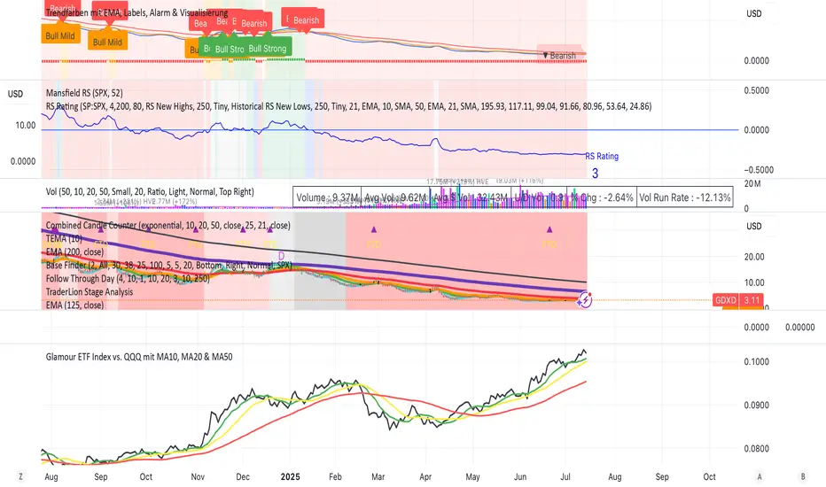
Glamour ETF Index vs. QQQ mit MA10, MA20 & MA50Stan Weinstein uses the term "Glamour Index" as a sentiment indicator to assess how speculative or overheated the stock market is. The Glamour Index measures the relationship between so-called "glamour stocks" (trendy stocks, hyped stocks with high media attention and sometimes extreme price increases) and solid, more conservative stocks. Weinstein uses this index to: 1) Analyze market sentiment – particularly whether the market is in a speculative euphoria phase.
2) Identify warning signs of a potential top formation or an impending downturn.
My basket compares performance against the QQQ (alternatively, SPY or any other benchmark is also possible).
My basket consists of the ETFs in the ARK universe, as well as other growth ETFs such as IPO, FFTY, and QQQJ.
Multi-TF Z-Score IndicatorIndicator to find the Z score for the daily 4h, 1h, 15m and 5 min time frames with 20 previous samples.


Fractal Pullback Market StructureFractal Pullback Market Structure
Author: The_Forex_Steward
License: Mozilla Public License 2.0
The Fractal Pullback Market Structure indicator is a sophisticated price action tool designed to visualize internal structure shifts and break-of-structure (BoS) events with high accuracy. It leverages fractal pullback logic to identify market swing points and confirm whether a directional change has occurred.
This indicator detects swing highs and lows based on fractal behavior, drawing zigzag lines to connect these key pivot points. It classifies and labels each structural point as either a Higher High (HH), Higher Low (HL), Lower High (LH), or Lower Low (LL). Internal shifts are marked using triangle symbols on the chart, distinguishing bullish from bearish developments.
Break of Structure events are confirmed when price closes beyond the most recent swing high or low, and a horizontal line is drawn at the breakout level. This helps traders validate when a structural trend change is underway.
Users can configure the lookback period that defines the sensitivity of the pullback detection, as well as a timeframe multiplier to align the logic with higher timeframes such as 4H or Daily. There are visual customization settings for the zigzag lines and BoS markers, including color, width, and style (solid, dotted, or dashed).
Alerts are available for each key structural label—HH, HL, LH, LL—as well as for BoS events. These alerts are filtered through a selectable alert mode that separates signals by timeframe category: Low Timeframe (LTF), Medium Timeframe (MTF), and High Timeframe (HTF). Each mode allows the user to receive alerts only when relevant to their strategy.
This indicator excels in trend confirmation and reversal detection. Traders can use it to identify developing structure, validate internal shifts, and anticipate breakout continuation or rejection. It is particularly useful for Smart Money Concept (SMC) traders, swing traders, and those looking to refine entries and exits based on price structure rather than lagging indicators.
Visual clarity, adaptable timeframe logic, and precise structural event detection make this tool a valuable addition to any price action trader’s toolkit.

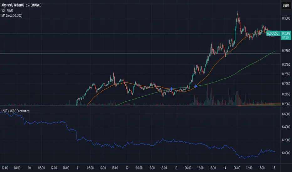
USDT + USDC DominanceUSDT and USDC Dominance: This refers to the combined market capitalization of Tether (USDT) and USD Coin (USDC) as a percentage of the total cryptocurrency market capitalization. It measures the proportion of the crypto market held by these stablecoins, which are pegged to the US dollar. High dominance indicates a "risk-off" sentiment, where investors hold stablecoins for safety during market uncertainty. A drop in dominance suggests capital is flowing into riskier assets like altcoins, often signaling a bullish market or the start of an "alt season."
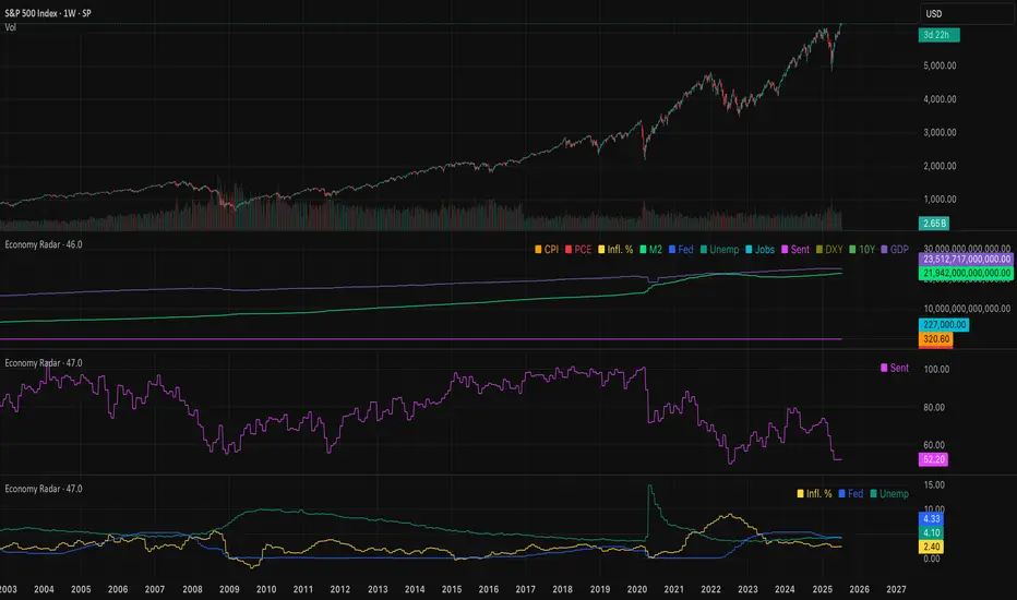
Economy RadarEconomy Radar — Key US Macro Indicators Visualized
A handy tool for traders and investors to monitor major US economic data in one chart.
Includes:
Inflation: CPI, PCE, yearly %, expectations
Monetary policy: Fed funds rate, M2 money supply
Labor market: Unemployment, jobless claims, consumer sentiment
Economy & markets: GDP, 10Y yield, US Dollar Index (DXY)
Options:
Toggle indicators on/off
Customizable colors
Tooltips explain each metric (in Russian & English)
Perfect for spotting economic cycles and supporting trading decisions.
Add to your chart and get a clear macro picture instantly!
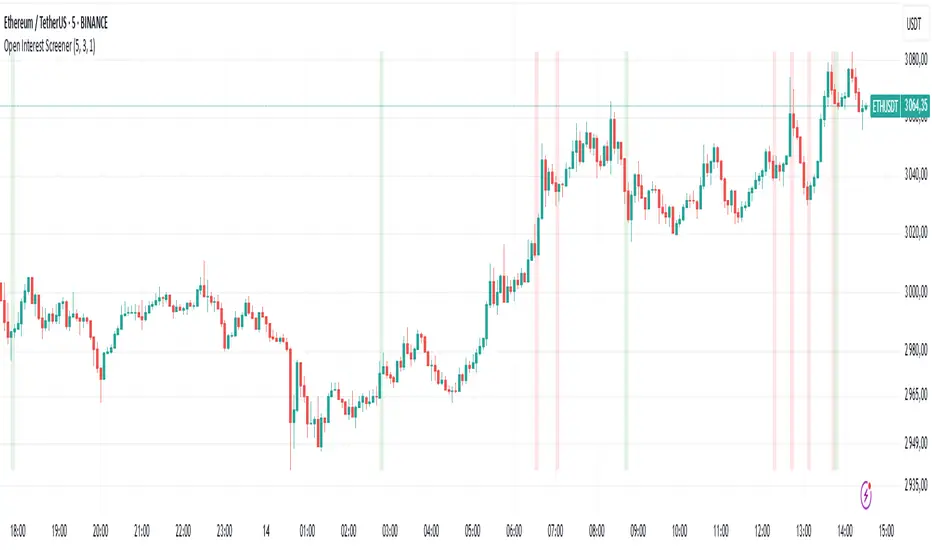
Open Interest Screener
Open Interest Screener
Traders often wonder: how do you enter a trend before it takes off — not at the very peak? Most classic technical indicators lag behind price. So what could you add to your system to catch a move earlier?
🔍 Enter the Open Interest Screener!
I've personally relied on this metric for years while trading crypto. It helps detect abnormal spikes in open interest — sudden increases in the number of outstanding derivative contracts — which often signal that something big is about to happen. These moments can mark the very start of a major trend.
🧠 How to use it:
Go long if price is rising and there's a spike in open interest on the way up.
Go short if price is falling and open interest rises during the decline.
Exit positions when open interest sharply drops — this may indicate the move is losing momentum.
⚙️ Settings & Customization:
Bars to look back — defines how far back the script looks to detect % changes in open interest.
OI % Change Threshold — adjust this to control sensitivity; higher = fewer, stronger signals.
Exchange source toggles — choose between BitMEX (USD/USDT) and Kraken data feeds.
Show Spike Zones — enable or disable visual highlights for detected spikes.
📌 Tips:
Configure the indicator for your preferred cryptocurrency pair and timeframe.
Visually validate that the OI spikes look meaningful and are not cluttering the chart.
Optimal settings vary by asset — take time to test and tune them for each coin.
With this tool, you're no longer guessing where the trend might begin — you're tracking the intent of market participants as it unfolds. Use it as part of a broader system and stay ahead of the herd.
USDT + USDC Dominance USDT + USDC Dominance: This refers to the combined market capitalization of Tether (USDT) and USD Coin (USDC) as a percentage of the total cryptocurrency market capitalization. It measures the proportion of the crypto market held by these stablecoins, which are pegged to the US dollar. High dominance indicates a "risk-off" sentiment, where investors hold stablecoins for safety during market uncertainty. A drop in dominance suggests capital is flowing into riskier assets like altcoins, often signaling a bullish market or the start of an "alt season.

RSI(14) Custom by ChadRSI 14 : this indicator works in low time frame like 1h and 4h, for entry long position and short position. when the line touch 70 mean the price is overbought, when the line touch 50 it"s neutral, and when the line touch 30 mean price is oversold.

[Enhanced] L1 Banker Move🧠 L1 Banker Move
This is a multi-layered momentum signal tool designed to reveal institutional activity before major price moves. It combines deep liquidity detection, price pressure dynamics, and short-term investor alignment to deliver actionable signals with clarity and precision.
Key Features:
🔴 Institutional Signal
Detects potential Level 1 banker moves based on deep price compression and long-term sweep logic (Lowest Low 90 + smoothed momentum spikes).
🔵 Institutional Build Phase
Shows stealth accumulation/distribution zones using low volatility buildup and compression-based ratios over the past 30 bars.
🟢 Short-Term Investor Signal
Confirms price shifts with VWAP cross, SMA structure, and fast/slow EMA delta acceleration. Useful for timing precision entries after institutional setups.
💜 Combined Strength Histogram
A composite momentum bar that blends all three layers to visually rank the power of each setup.
🎯 Smart Highlighting & Alerts
Background turns red when an institutional signal appears without retail confirmation—flagging early entry traps or front-running zones. Includes alert conditions to notify you of optimal entry moments.
Customization:
Adjust the EMA delta sensitivity
Choose your preferred institutional timeframe (default: Daily)

[Enhanced] L1 Banker MoveThis is a multi-layered momentum signal tool designed to reveal institutional activity before major price moves. It combines deep liquidity detection, price pressure dynamics, and short-term investor alignment to deliver actionable signals with clarity and precision.
Key Features:
🔴 Institutional Signal
Detects potential Level 1 banker moves based on deep price compression and long-term sweep logic (Lowest Low 90 + smoothed momentum spikes).
🔵 Institutional Build Phase
Shows stealth accumulation/distribution zones using low volatility buildup and compression-based ratios over the past 30 bars.
🟢 Short-Term Investor Signal
Confirms price shifts with VWAP cross, SMA structure, and fast/slow EMA delta acceleration. Useful for timing precision entries after institutional setups.
💜 Combined Strength Histogram
A composite momentum bar that blends all three layers to visually rank the power of each setup.
🎯 Smart Highlighting & Alerts
Background turns red when an institutional signal appears without retail confirmation—flagging early entry traps or front-running zones. Includes alert conditions to notify you of optimal entry moments.
Customization:
Adjust the EMA delta sensitivity
Choose your preferred institutional timeframe (default: Daily)

Inverted USDT.DSignal Logic at a Glance
Exits happen automatically if price crosses EMA200 in the opposite direction, or whenever any SAR cross occurs (strict stop on your “risky” trades).
The indicator’s core logic uses a 200-period EMA crossover on USDT.D (and optionally VIX) to define the primary trend—price crossing above the EMA closes shorts and opens longs, while crossing below does the opposite—and then layers on “risky” entries whenever the Parabolic SAR flips within that trend (SAR dot appearing below price in an uptrend for add-on longs, above price in a downtrend for add-on shorts). All positions—main and risky—are closed automatically if price crosses the EMA against your trade or any SAR cross occurs. An invert toggle flips every entry/exit rule, letting you trade the opposite signals, and identical logic runs in parallel on VIX to offer complementary or hedged signals.
Step-by-Step Usage Example
1. Set your timeframe (e.g., Daily or 4H).
2. Watch for the Main Long label (green arrow up).
3. When it appears, the strategy will close any short and open a new long.
4. Optionally, use a Sar Long label as a signal to add to your position.
5. Stay in the trade while price remains above EMA200.
6. Exit on either a Main Short or when SAR flips against you.
Tips for Real-World Trading
• Turn on alerts for each label type so you never miss a signal.
• Use the built-in Strategy Tester to optimize your SAR parameters and position sizing.
• Combine with a fixed stop-loss or take-profit discipline off-chart.
• Experiment with the Invert Signal toggle in different market regimes.
