Top Performer Dashboard (22 Stocks)added to your chart you can add up to 22 individual stocks, it will rank them from highest to lowest growth over 4 time frames, 1 week, 1 month, 3 month and 6 months. you can sort the results by each time frame.
please enjoy
"top" için komut dosyalarını ara

Daily ATR vs Move (black & white) + PipsTop of Chart, Mid. Gives the user an idea of what trend is doing and how the current price compares to daily ATR.
Used on this example below to indicate we are within the bottom range for the day, and price has potential to move up without worry of exhaustion.

[Top] Simple ATR TP/SLSimple TP/SL from ATR (Locked per Bar) - Advanced Position Management Tool
What This Indicator Does:
Automatically calculates and displays Take Profit (TP) and Stop Loss (SL) levels based on Average True Range (ATR)
Locks ATR values and direction signals at the start of each bar to prevent repainting and provide consistent levels
Offers multiple direction detection modes including real-time candle-based positioning for dynamic trading approaches
Displays entry, TP, and SL levels as clean horizontal lines that extend from the current bar
Original Features That Make This Script Unique:
Bar-Locked ATR System: ATR values are captured and frozen at bar open, ensuring levels remain stable throughout the bar's progression
Multi-Modal Direction Detection: Four distinct modes for determining TP/SL positioning - Trend Following (EMA-based), Bullish Only, Bearish Only, and real-time Candle Based
Real-Time Candle Flipping: In Candle Based mode, TP/SL levels flip immediately when the current candle changes from bullish to bearish or vice versa
Persistent Line Management: Uses efficient line object management to prevent ghost lines and maintain clean visual presentation
Flexible Base Price Selection: Choose between Open (static), Close (dynamic), or midpoint (H+L)/2 for entry level calculation
How The Algorithm Works:
ATR Calculation: Captures ATR value at each bar open using specified length parameter, maintaining consistency throughout the bar
Direction Determination: Uses different methods based on selected mode - EMA crossover for trend following, or real-time candle color for dynamic positioning
Level Calculation: TP level = Base Price + (Direction × TP Multiplier × ATR), SL level = Base Price - (Direction × SL Multiplier × ATR)
Visual Management: Creates persistent line objects once, then updates their positions every bar for optimal performance
Direction Modes Explained:
Trend Following: Uses 5-period and 12-period EMA relationship to determine trend direction (locked at bar open)
Bullish Only: Always places TP above and SL below entry (traditional long setup)
Bearish Only: Always places TP below and SL above entry (traditional short setup)
Candle Based: Dynamically adjusts based on current candle direction - flips in real-time as candle develops
Key Input Parameters:
ATR Length: Period for ATR calculation (default 14) - longer periods provide smoother volatility measurement
TP Multiplier: Take profit distance as multiple of ATR (default 1.0) - higher values target larger profits
SL Multiplier: Stop loss distance as multiple of ATR (default 1.0) - higher values allow more room for price movement
Base Price: Reference point for level calculations - Open for static entry, Close for dynamic tracking
Direction Mode: Method for determining whether TP goes above or below entry level
How To Use This Indicator:
For Position Sizing: Use the displayed SL distance to calculate appropriate position size based on your risk tolerance
For Entry Timing: Wait for price to approach the entry level before taking positions
For Risk Management: Set your actual stop loss orders at or near the displayed SL level
For Profit Taking: Use the TP level as initial profit target, consider scaling out at this level
Mode Selection: Choose Candle Based for scalping and quick reversals, Trend Following for swing trading
Visual Style Customization:
Line Colors: Customize TP line color (default teal) and SL line color (default orange) for easy identification
Line Widths: Adjust TP/SL line thickness (1-5) and entry line thickness (1-3) for visibility preferences
Clean Display: Lines extend 3 bars forward from current bar and update position dynamically
Best Practices:
Use on clean charts without multiple overlapping indicators for clearest visual interpretation
Combine with volume analysis and key support/resistance levels for enhanced decision making
Adjust ATR length based on your trading timeframe - shorter for scalping, longer for position trading
Test different TP/SL multipliers based on the volatility characteristics of your chosen instruments
Consider using Trend Following mode during strong trending periods and Candle Based during ranging markets

[Top] LHAMA Consolidation DetectorIntroducing the Low-High Adaptive Moving Average (LHAMA 🦙), a powerful tool designed to help traders visually distinguish between trending and consolidating market phases. Unlike traditional moving averages that can produce false signals in choppy markets, the LHAMA is engineered to flatten out during periods of consolidation and become more responsive when a clear trend emerges.
This indicator's primary function is to act as a "Consolidation Detector." When the LHAMA line goes flat and adopts its "Flat Color," it serves as a clear visual cue that the market is range-bound. Conversely, when the line begins to slope and changes to its Bullish or Bearish color, it signals a potential breakout or the start of a new trend.
How It Works
The LHAMA is a type of adaptive moving average. Its adaptiveness is derived from a unique calculation that measures market "trendiness." It does this by tracking whether new highs or new lows are being made within a specified lookback period.
In a Trending Market: When the price consistently makes new highs or lows, the indicator's responsiveness increases, causing the LHAMA to track the price much more closely and responsively.
In a Consolidating Market: When the price is range-bound and fails to make new highs or lows, the responsiveness decreases significantly. This causes the LHAMA to flatten out and become less sensitive to minor price fluctuations, effectively filtering out market noise.
Key Features
Adaptive Calculation: The core engine of the indicator, which automatically adjusts its smoothing based on trend strength.
Slope-Based Coloring: The line's color dynamically changes based on its slope, providing an at-a-glance view of market conditions: bullish, bearish, or flat.
Multi-Line & Multi-Timeframe (MTF): You can enable up to six fully customizable LHAMA lines. Each line can be configured with its own length, colors, and can even be set to a different timeframe, allowing for comprehensive multi-timeframe analysis on a single chart.
Volatility Clouds: Each LHAMA can display an optional cloud around it. The cloud's width is based on your choice of either the Average True Range (ATR) or Standard Deviation (StdDev), offering a visual representation of volatility.
Volume Weighting: An option to incorporate volume into the adaptive calculation, making the LHAMA even more responsive during high-volume price movements.
How to Use
Identify Consolidation: The primary use case. A flat and consistently colored LHAMA line is a strong indication of a sideways or consolidating market. This can help traders avoid taking trend-following trades in choppy conditions.
Confirm Trends: When the LHAMA begins to slope upwards or downwards and changes to its trend color, it can be used to confirm the direction and strength of a new trend. The steeper the slope, the stronger the momentum, and more solid the directional color.
Dynamic Support & Resistance: Like other moving averages, the LHAMA can act as a dynamic level of support in an uptrend or resistance in a downtrend. The optional cloud can further define these zones.
Multi-MA Ribbon Strategy: By enabling multiple LHAMAs with different lengths (e.g., Fibonacci sequence like 14, 21, 34, 55), you can create a ribbon. The expansion of the ribbon indicates a strong trend, while its contraction signals a weakening trend or consolidation.
Settings Explained
Enable 🦙 Line: A simple checkbox to turn each of the six LHAMA lines on or off.
Length: The lookback period for the LHAMA calculation. Shorter lengths are more responsive, while longer lengths are smoother.
Timeframe: Set a specific timeframe for each LHAMA. Leave blank to use the chart's current timeframe.
Volume Weight: If checked, adds volume weighting to make the LHAMA more responsive to high-volume moves.
Colors (Bullish, Bearish, Flat): Customize the colors for each market state. To only see the line during consolidation, set the Bullish and Bearish colors to 100% transparency. To hide the line during consolidation, set the Flat color to 100% transparency.
Color Sensitivity: This is a crucial setting. Because price scales (tick sizes) vary widely between symbols, this setting allows you to adjust the sensitivity of the slope detection. A lower value requires a steeper slope to trigger a trend color, while a higher value is more sensitive.
Recommended settings are provided in the input tooltip as a starting point:
$5 Tick: 0.25 Sensitivity
$1 Tick: 0.75 Sensitivity
$0.25 Tick: 3 Sensitivity
$0.01 Tick: 50 Sensitivity
$0.005 Tick: 100 Sensitivity
Cloud Settings:
Show Cloud: Toggles the visibility of the volatility cloud around the LHAMA.
Width Based On: Choose between "ATR" or "StdDev" to calculate the cloud's width.
Cloud Length & Width: Set the lookback period and multiplier for the ATR/StdDev calculation to control the size of the cloud.
Top - Bottom Using MAThis script is used decide weather stock is overbought or oversold in given length/days from the settings.
using close difference from ohlc4 moving average ratio.
Settings Available
1) moving average length
2) Highest / Lowest ratio length
3) Difference Between Highest and Lowest Line
this script plot/display 4 lines
1) highest difference from moving averages in provided length.
2) lowest difference from moving averages in provided length.
3) ratio of moving average and ohlc4
4) linear regression moving averages of ratio of moving average and ohlc4
How to use this script
1) when ratio line is touch 2 days to highest ratio line means we are consider stock is in overbought levels or linear regression moving average above highest ratio line means overbought.
2) when ratio lines cross below its linear regression moving average then we consider final exit or book profit.
3) when linear regression moving average below lowest ratio line means stock is in oversold.
4) when linear regression moving average below lowest ratio line and linear regression line start rising after fall it means there is change in trend.
5) when linear regression moving average cross above lowest ratio line it means trend is changed and linear regression line turns green.

TOP 4 STABLECOIN MARKET CAPIn the cryptocurrency market, there is a challenge: understanding the flow of stablecoins during market growth and downturns. It's difficult to grasp whether the market surge is due to a shift in funds from BTC or an influx of USD. Detecting the fluctuation in market capitalization of stablecoins helps investors gain a clearer perspective of market volatility.
Usage:
When there are fluctuations in the market capitalization, it is essential to combine observations of this indicator with other technical indicators.

ADR in 0.5 / 1 / 3 / 5top of the morning!
This indicator is a tiny bit different then the previous one i published.
As per my little study into the ATR, i have decided to remove it out of my indicator and instead put in a half an ADR in dollar vallue.
For me, i can use this value to check at what level i would like my stop. The next evolvement of this indicator might be a total new one since i'd be one for a lower timeframe with the 0.5 and 0.3 adr down from current high otd.
Hope you enjoy it,
Peace

Top 5 Power Momentum IndicatorHow I Never Trade Against the Trend
"Today I want to reveal another amazing tool in my arsenal when it comes to intraday trading. Now this is only for intraday time frames and not for swings or anything longer than few minutes to few hours ."
from Tic Tock Trading Substack
credit to Vincente

COVID19 in % of the population of this countryTop 10 countries by the number of infected #COVID19 (#coronavirus) as a % of the population of this country.


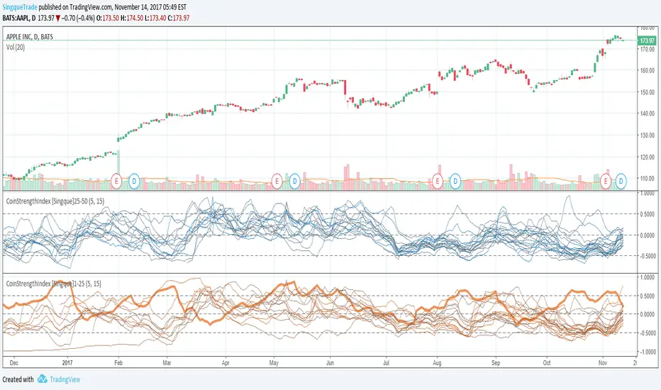
CoinStrengthIndex [Singque]1-25Top 1-25 market cap altcoins true strength. Color gradient red to blue based on highest cap to lowest cap. Enjoy.(Use with bitcoin chart)
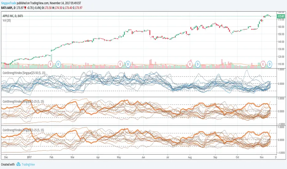
CoinStrengthIndex [Singque]25-50Top 25-30 market cap altcoins true strength. Color gradient red to blue based on highest cap to lowest cap. Enjoy. (Use with bitcoin chart)
Smart Adaptive Double Patterns [The_lurker]Smart Adaptive Double Patterns
This is an advanced technical indicator that combines two of the strongest and most renowned classical price reversal patterns:
✅ Double Bottom Pattern — a bullish reversal pattern that forms after a downtrend
✅ Double Top Pattern — a bearish reversal pattern that forms after an uptrend
The indicator does not merely detect patterns — it provides a fully integrated, intelligent system that includes:
✅ Precise quality scoring for each pattern using 5 technical criteria
✅ Automatic price target calculation at three levels (Conservative, Balanced, Aggressive)
✅ Multi-layer dynamic filtering to avoid false signals
✅ Live pattern tracking from formation to target achievement or failure
✅ Comprehensive alert system covering all possible trading scenarios
🎯 Why Is This Indicator Unique?
1️⃣ High Detection Accuracy
Unlike traditional indicators that rely on simple rules, this one applies 5 strict structural conditions to confirm pattern validity:
A clear trend must precede the pattern
High symmetry between the two bottoms or two tops
No break of critical price levels during formation
Logical spacing between key points
Technical confirmation from ADX, ATR, and Volume
2️⃣ Advanced Quality Scoring System
Each pattern is scored out of 100 based on 5 weighted criteria:
Symmetry (30%): How closely the two bottoms or tops match
Trend Strength (20%): Strength of the prior trend
Volume Behavior (20%): Trading activity at critical points
Pattern Depth (15%): Vertical distance between neckline and bottom/top
Structural Integrity (15%): Full compliance with structural rules
3️⃣ Smart Target Management
Separate targets for bullish (Double Bottom) and bearish (Double Top) patterns
Separate projections for success and failure cases
Multiple options: Conservative (0.618) / Balanced (1.0) / Aggressive (1.618)
Live tracking with dynamic moving lines
4️⃣ Professional Failure Handling
Failed patterns are not ignored — they are turned into counter-trend opportunities:
Failed Double Bottom → triggers a bearish signal with downside targets
Failed Double Top → triggers a bullish signal with upside targets
Automatic color change for clear visual distinction
5️⃣ Full Customization Flexibility
Enable/disable each pattern independently
22+ adjustable settings
Unique colors for each pattern and quality level
Full bilingual support (Arabic / English)
📐 Pattern Details
🟦 Double Bottom Pattern
Sequence of points:
🔹 Point 1: Peak marking the start of a strong downtrend
🔹 Point 2 (Bottom 1): First low — first key bounce
🔹 Point 3: Intermediate high — forms the neckline (resistance)
🔹 Point 4 (Bottom 2): Second low — should closely match Bottom 1
🔹 Point 5: Breakout point — pattern confirmation
Mandatory Conditions:
✅ Clear downtrend before Point 2
✅ Bottoms 2 & 4 nearly identical (≤1.5% difference by default)
✅ Point 3 higher than both bottoms
✅ Neither bottom is broken during formation
✅ Sufficient time between points (≥10 candles by default)
✅ Success Scenario
→ Price breaks above the neckline (Point 3)
→ Point 5 is plotted at breakout candle
→ Dashed vertical line drawn from Point 5 to target
→ Horizontal dashed line tracks price toward target
→ Dashboard shows: Pattern Type | Quality | Rating | Target | Status
→ When target hits: line turns green + ✅ appears
🎯 Target Calculation
Pattern Height = Point 3 − Point 4
• Conservative: Point 3 + (Height × 0.618 × Quality Factor)
• Balanced: Point 3 + (Height × 1.0 × Quality Factor)
• Aggressive: Point 3 + (Height × 1.618 × Quality Factor)
❌ Failure Scenario
→ Price breaks below both Bottom 1 or Bottom 2 before neckline breakout
Visual Changes:
All lines turn red
Red ✖ appears at breakdown candle
Neckline stops expanding
Red dashed vertical line from breakdown point to bearish target
Red horizontal tracking line follows price
Dashboard updates to:
⚠ Failed Bottom – Bearish
→ Shows new bearish target
→ Indicates target mode for failure case
→ Status: Bearish Reversal
→ Fully red display
🟥 Double Top Pattern
Sequence of points:
🔹 Point 1: Trough marking the start of a strong uptrend
🔹 Point 2 (Top 1): First peak — first key resistance
🔹 Point 3: Intermediate low — forms the neckline (support)
🔹 Point 4 (Top 2): Second peak — should closely match Top 1
🔹 Point 5: Breakdown point — pattern confirmation
Mandatory Conditions:
✅ Clear uptrend before Point 2
✅ Tops 2 & 4 nearly identical (≤1.5% difference by default)
✅ Point 3 lower than both tops
✅ Neither top is breached during formation
✅ Sufficient time between points (≥10 candles by default)
✅ Success Scenario
→ Price breaks below the neckline (Point 3)
→ Point 5 is plotted at breakdown candle
→ Dashed vertical line drawn to target
→ Horizontal tracking line moves with price
→ Dashboard updates accordingly
→ Green line + ✅ on hit
🎯 Target Calculation
Pattern Height = Point 4 − Point 3
• Conservative: Point 3 − (Height × 0.618 × Quality Factor)
• Balanced: Point 3 − (Height × 1.0 × Quality Factor)
• Aggressive: Point 3 − (Height × 1.618 × Quality Factor)
❌ Failure Scenario
→ Price breaks above either Top 1 or Top 2 before neckline breakdown
Visual Changes:
All lines turn cyan (light blue)
Cyan ✖ appears at breakout candle
Neckline stops expanding
Cyan dashed vertical line to bullish target
Cyan horizontal tracking line follows price
Dashboard updates to:
⚠ Failed Top – Bullish
→ Shows new bullish target
→ Indicates target mode for failure case
→ Status: Bullish Reversal
→ Fully cyan display
🎯 Upside Target (after Double Top failure)
Max Top = max(Point 2, Point 4)
Height = Max Top − Point 3
• Conservative: Max Top + (Height × 0.618)
• Balanced: Max Top + (Height × 1.0)
• Aggressive: Max Top + (Height × 1.618)
📊 Quality Scoring System (0–100)
1️⃣ Symmetry (30%)
Measures price match between the two bottoms or two tops.
High score (25–30): Near-perfect symmetry → very strong pattern
Medium (15–24): Good match → reliable signal
Low (5–14): Weak symmetry → use caution
Zero: No symmetry → invalid pattern
2️⃣ Trend Strength (20%)
Uses ADX and DI indicators.
20 pts: Strong trend confirmed (e.g., ADX ≥ 20 + correct DI alignment)
10 pts: Trend filter disabled
6 pts: Weak or sideways trend
3️⃣ Volume Behavior (20%)
Declining volume on second touch is a positive sign (shows exhaustion).
15–20 pts: Clear volume drop → strong signal
10 pts: Neutral volume
6 pts: Rising volume → higher risk of continuation
4️⃣ Pattern Depth (15%)
Deeper patterns = stronger reversals.
12–15 pts: Deep → high reversal power
8–11 pts: Medium → acceptable
<8 pts: Shallow → weak signal
5️⃣ Structural Integrity (15%)
Checks logical structure (e.g., Point 1 > Point 3 in Double Bottom).
12–15 pts: Ideal structure
8–11 pts: Minor flaws
<8 pts: Poor setup
📈 Final Quality Rating & Colors
• 85–100 → ⭐ Excellent
→ Double Bottom: Cyan #00BCD4
→ Double Top: Light Red #FF5252
• 75–84 → ✨ Very Good
• 65–74 → ✓ Good
• 60–64 → ○ Acceptable
→ All use Amber #FFC107
• <60 → ❌ Rejected (not shown)
→ Gray #9E9E9E
🔧 Dynamic Filters
1️⃣ ATR Filter (Volatility Check)
Rejects patterns in abnormally high volatility periods.
→ If current ATR > 1.8 × 50-period ATR MA → pattern rejected
✅ Recommended for crypto, small caps
❌ Optional for calm markets (gold, bonds)
2️⃣ ADX Filter (Trend Confirmation)
Ensures a real trend exists before the pattern.
→ If ADX < 14 (70% of default 20) → pattern rejected
✅ Strongly recommended (keep ON)
3️⃣ Volume Filter (Behavior Validation)
Not used to reject patterns, but strongly affects quality score.
✅ Best for liquid markets (Forex majors, large stocks)
❌ Optional for illiquid assets
⚙️ Key Settings Explained
🔘 General Settings
• Language: Arabic / English
• Show Previous Patterns: Yes / No
→ “No” keeps chart clean; “Yes” for historical review
🔘 Pattern Selection
• Enable Double Bottom: ✅ / ❌
• Enable Double Top: ✅ / ❌
→ Use combinations:
✅✅ → Full reversal scanning
✅❌ → Long setups only
❌✅ → Short setups only
❌❌ → Indicator OFF
🔘 Detection Parameters
• Pivots Left (1–20): Higher = more reliable, fewer patterns
• Pivots Right (1–20): Lower = faster signals
• Min Width (5–100): Min candles between Bottom/Top 1 & 2
• Tolerance % (0.1%–5%): Max allowed price difference
• Min Arm (5–50): Min candles between pivot & neckline
• Min Trend (5–50): Min candles in prior trend
• Trend Lookback (50–500): How far back to detect trend start
• Extension Multiplier (1.0–5.0): How long to wait for breakout
🔘 Quality Settings
• Min Quality Score (0–100):
→ Conservative: 75–85
→ Balanced: 60–70
→ Flexible: 50–55
• Custom Weights: Adjust based on market (e.g., increase Volume weight in Forex)
🔘 Target Settings
• Bottom Bullish Target: Conservative / Balanced / Aggressive
• Bottom Bearish Target: (used on failure)
• Top Bearish Target: Conservative / Balanced / Aggressive
• Top Bullish Target: (used on failure)
🔘 Visual Settings
• Label Size: Small / Normal / Large / Huge
• Pattern Colors: Fully customizable
• Table: Show/Hide + Size (Small/Normal/Large) + Position (Top-Right / Top-Left / Bottom-Right / Bottom-Left)
• Fill Transparency: 70%–95% (default: 85%)
🔔 Alert System (8 Independent Alerts)
📌 Double Bottom Alerts
Bullish Breakout → “Double Bottom Breakout – Bullish!”
Bullish Target Hit → “Bullish Target Achieved!”
Failure (Bearish) → “Double Bottom Failed – Bearish!”
Bearish Target Hit → “Bearish Target Achieved (Failure)!”
📌 Double Top Alerts
Bearish Breakdown → “Double Top Breakdown – Bearish!”
Bearish Target Hit → “Bearish Target Achieved!”
Failure (Bullish) → “Double Top Failed – Bullish!”
Bullish Target Hit → “Bullish Target Achieved (Failure)!”
Each alert can be enabled/disabled independently and supports pop-ups, emails, or webhooks.
⚠️ Disclaimer:
This indicator is for educational and analytical purposes only. It does not constitute financial, investment, or trading advice. Use it in conjunction with your own strategy and risk management. Neither TradingView nor the developer is liable for any financial decisions or losses.

Chart Patterns [ActiveQuants]The Chart Patterns indicator is a comprehensive tool designed to automatically identify a variety of common chart patterns directly on your price chart. By detecting sequences of pivot highs and lows , this indicator helps traders spot potential trend continuations , reversals , and key market structures such as Double Tops and Double Bottoms . Enhance your technical analysis by quickly recognizing these formations as they emerge.
How It Works
The indicator operates in a two-stage process:
Pivot Point Detection: It first identifies significant swing highs and swing lows (pivot points) based on a user-defined Period . These pivots form the fundamental building blocks for pattern recognition.
Pattern Recognition: Using the sequence of these detected pivot points, the script then applies logical rules to identify the following patterns:
Lower Low (LL)
Lower Low & Lower High (LL & LH)
Higher High (HH)
Higher High & Higher Low (HH & HL)
Double Tops
Double Bottoms
Patterns are drawn on the chart with connecting lines and labeled for easy identification. Double Tops and Double Bottoms also feature a status system: " Active " while forming, " Confirmed " upon neckline breakout, or " Invalid " if specific conditions negate the pattern before confirmation.
█ KEY FEATURES
Comprehensive Pattern Detection: Identifies six distinct types of chart patterns, offering insights into both trend continuation and potential reversals.
Pivot-Based Analysis: Uses a robust method of identifying pivot highs and lows as the foundation for pattern formation.
Pattern Status for Double Tops/Bottoms:
- Active: A Double Top or Double Bottom pattern has formed its two peaks/troughs and the intervening neckline point, but the price has not yet broken beyond the neckline. The pattern is developing .
- Confirmed: The price has decisively closed beyond the neckline (below for Double Top, above for Double Bottom), signaling a potential entry or validation of the pattern.
- Invalid: An " Active " Double Top or Double Bottom pattern can be invalidated if, before a neckline breakout occurs, a new pivot point forms that negates the pattern’s structural integrity. For example, if a new pivot low forms above or at the neckline of an Active Double Top, the pattern is considered invalid because the market failed to break down and instead showed relative strength.
Customizable Visuals: Allows users to define colors for bullish and bearish patterns, line widths, and the visibility of pivot points.
Selective Pattern Display: Users can choose to display all patterns or filter by status (Active, Confirmed, Invalid) for Double Tops/Bottoms. Individual pattern types can also be toggled on or off.
Historical Analysis Control: The Show Last History (Bars) input allows users to specify how far back the indicator should plot patterns, optimizing performance and chart readability.
Clear Labeling: Patterns are clearly labeled on the chart, with Double Tops/Bottoms also showing " Top 1 ," " Top 2 ," or " Bottom 1 ," " Bottom 2 " labels.
█ PATTERNS DETECTED
Lower Low (LL): Indicates a potential bearish continuation or the start of a downtrend. Forms when price makes a lower low during an uptrend.
Lower Low & Lower High (LL & LH): A stronger confirmation of a bearish trend, where the market forms a lower low followed by a lower high .
Higher High (HH): Signals a potential bullish continuation or the start of an uptrend. Forms when price makes a higher high during a downtrend.
Higher High & Higher Low (HH & HL): A stronger confirmation of a bullish trend, where the market forms a higher high followed by a higher low .
Double Top: A bearish reversal pattern characterized by two distinct peaks at roughly the same price level, separated by a trough (neckline). Confirmation occurs when price breaks below the neckline.
Double Bottom: A bullish reversal pattern featuring two distinct troughs at roughly the same price level, separated by a peak (neckline). Confirmation occurs when price breaks above the neckline.
█ EXAMPLE: DOUBLE TOP INVALIDATION
Understanding how a Double Top or Double Bottom can be invalidated is crucial. Here's an example for a Double Top:
Formation: The indicator identifies two peaks (Top 1, Top 2) at a similar price level, with a corrective trough (Neckline Pivot P5) in between. The pattern is labeled " Double Top " and is in an " Active " state. ( Imagine points P4 and P6 are the two tops, and P5 is the low point of the neckline between them ).
Pre-Breakout Condition: The price action continues, but before it breaks decisively below the P5 neckline level, a new significant swing low (a new pivot low) forms.
Invalidation Check: The indicator checks the price level of this new pivot low. If this new pivot low occurs at a price equal to or higher than the P5 neckline level, the " Active " Double Top pattern is re-labeled as " Invalid Double Top ". ( See image below for a visual representation of this scenario )
In this example, the Double Top formed with Top 1 (P4) and Top 2 (P6). The neckline is at P5. Before price broke below P5, a new pivot low formed at the red circle. Since this new pivot low is above the P5 neckline, the Double Top is marked " Invalid ".
The logic is that the market failed to break the neckline support and instead established a higher low (or a low at the support level), suggesting that the immediate bearish pressure has waned, thus invalidating the bearish reversal implication of the Double Top before it could confirm. A similar logic applies to Double Bottoms (a new pivot high forming below or at the neckline before an upside breakout).
█ USER INPUTS
Visibility and Common Styling
- Show Last History (Bars):
Specifies the number of recent bars the indicator will analyze and plot patterns on.
Default: 3000 bars. Min: 10.
- Patterns:
Filters which patterns are displayed based on their status.
Options: All, Active, Confirmed, Invalid.
Default: All.
- Pattern Line Width:
Sets the thickness of the lines used to draw the patterns.
Default: 1. Min: 1, Max: 10.
- Bearish Color:
Color for bearish patterns (LL, LL & LH, Double Tops).
Default: Red.
- Bullish Color:
Color for bullish patterns (HH, HH & HL, Double Bottoms).
Default: Green.
Pivot Points
- Period:
The lookback period on either side of a bar to qualify it as a pivot high or low. Higher values detect more significant pivots.
Default: 10 bars. Min: 2.
- Show Pivot Highs:
Toggles the visibility of detected pivot high markers.
Default: Enabled.
- Show Pivot Lows:
Toggles the visibility of detected pivot low markers.
Default: Enabled.
- Pivot Highs Color:
Color for the pivot high markers.
Default: #ff5252 (Reddish).
- Pivot Lows Color:
Color for the pivot low markers.
Default: #089981 (Greenish).
Patterns (Toggles)
- Lower Low:
Enable/disable detection and display of Lower Low patterns.
Default: Enabled.
- Lower Low & Lower High:
Enable/disable detection and display of Lower Low & Lower High patterns.
Default: Enabled.
- Higher High:
Enable/disable detection and display of Higher High patterns.
Default: Enabled.
- Higher High & Higher Low:
Enable/disable detection and display of Higher High & Higher Low patterns.
Default: Enabled.
- Double Tops:
Enable/disable detection and display of Double Top patterns.
Default: Enabled.
- Double Bottoms:
Enable/disable detection and display of Double Bottom patterns.
Default: Enabled.
█ CONCLUSION
The Chart Patterns indicator is a versatile and powerful assistant for traders who utilize classical chart pattern analysis. By automating the detection of key formations and providing clear visual cues along with status updates for patterns like Double Tops and Bottoms, it allows traders to focus on strategy development and execution. With its customizable settings, it can be adapted to various instruments and timeframes, making it a valuable addition to any technical trader's toolkit.
█ IMPORTANT NOTES
⚠ Pivot Period Sensitivity: The Period setting for pivot detection is crucial. A shorter period will identify more frequent, smaller swings, while a longer period will focus on more significant turning points. Adjust this setting based on the asset's volatility, the timeframe you are trading and your trading style.
⚠ Confirmation is Key: While the indicator identifies patterns, always wait for pattern confirmation (e.g., neckline breaks for Double Tops/Bottoms) and consider other factors like volume and market context before making trading decisions.
⚠ Confirmed Bars for Detection: Patterns are identified based on confirmed pivot points, which means a pivot is recognized period bars after it has formed. Status updates for Double Tops/Bottoms (Active, Confirmed, Invalid) also occur on confirmed bars. This approach enhances reliability and reduces the likelihood of repainting based on intra-bar price fluctuations.
⚠ Not a Standalone System: Chart patterns provide valuable insights, but they should be used in conjunction with other technical analysis tools (e.g., trendlines, moving averages, oscillators) and a sound risk management plan.
⚠ Lagging Nature: By their very definition, chart patterns are lagging indicators as they require a sequence of price action and several pivot points to complete their formation.
█ RISK DISCLAIMER
Trading involves a substantial risk of loss and is not suitable for every investor. The information provided by the Chart Patterns indicator is for educational and informational purposes only. It should not be considered as financial advice or a recommendation to buy or sell any security. Chart patterns indicate potential price movements but do not guarantee future results. Always perform your own due diligence and consult with a qualified financial advisor before making any investment decisions. Past performance is not indicative of future results.
📈 Happy trading! 🚀

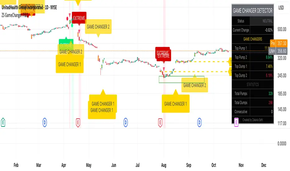
ZS Game Changer Pump & Dump DetectorZS GAME CHANGER PUMP AND DUMP DETECTOR - TOP 2 MOMENTUM TRACKER
Created by Zakaria Safri
An intelligent indicator specifically designed to identify and highlight the two most significant pump and dump candles within your selected lookback period. Perfect for traders who want to focus on the game-changing moves that truly matter in volatile markets like cryptocurrency, stocks, and forex.
CORE FEATURES
AUTOMATIC GAME CHANGER DETECTION
The indicator continuously scans your specified lookback period and automatically identifies the top 2 strongest pump candles and top 2 strongest dump candles. These game-changing candles are highlighted with distinctive gold labels and horizontal reference lines, making them instantly visible on your chart. Unlike other indicators that show every small move, this focuses exclusively on the market-moving moments that define trends and create opportunities.
INTELLIGENT PUMP AND DUMP CLASSIFICATION
Uses advanced percentage-based calculations to classify candles as pumps when price surges significantly upward and dumps when price plunges sharply downward. The detection system accounts for candle body size, wick proportions, and volume confirmation to ensure only legitimate momentum moves trigger signals. Customizable thresholds allow adaptation to any market volatility profile from calm stocks to wild altcoins.
ADVANCED WICK EXCLUSION FILTER
Eliminates false signals caused by candles with large wicks and small bodies. This filter focuses analysis exclusively on candles with substantial body sizes that indicate genuine directional conviction rather than temporary spikes followed by rejection. The body to candle ratio is fully adjustable to match your preferred signal quality standards.
VOLUME CONFIRMATION SYSTEM
Optional volume filter ensures detected pumps and dumps are backed by real market participation. The indicator compares current volume against a moving average and only triggers signals when volume exceeds your specified multiplier threshold. This eliminates low-volume noise and focuses on moves supported by institutional or crowd participation.
RALLY SEQUENCE DETECTION
Identifies and highlights consecutive sequences of pump or dump candles with colored background overlays. Green background indicates sustained buying pressure across multiple candles while red background shows sustained selling pressure. The rally detection system includes an optional one-miss allowance that prevents the sequence from breaking due to a single neutral candle.
HORIZONTAL REFERENCE LINES
Draws dashed lines from each game changer candle extending to the current bar, providing constant visual reference to the most significant support and resistance levels created by extreme momentum. The top game changer gets a thick dashed line while the second gets a dotted line for easy differentiation. Labels on the right side display the exact percentage move.
COMPREHENSIVE STATISTICS DASHBOARD
Real-time information panel showing current market status as pumping, dumping, or neutral along with the current candle percentage change. Displays the exact percentage values for top pump number 1, top pump number 2, top dump number 1, and top dump number 2. Shows running totals of all pumps and dumps detected since chart load. Tracks consecutive candle counts during active rally sequences.
TESTING AND VERIFICATION MODE
Built-in debug mode displays percentage change directly on each qualifying pump and dump candle, allowing instant verification that calculations are accurate. Shows which filters are currently active with a simple code in the dashboard. Helps traders understand exactly why certain candles qualified as game changers.
HOW THE GAME CHANGER DETECTION WORKS
SCANNING ALGORITHM
Every bar close, the indicator scans backward through your specified lookback period examining every candle's percentage change from its previous close. For bullish moves, it identifies the two candles with the largest positive percentage change that meet your threshold requirements. For bearish moves, it identifies the two candles with the largest negative percentage change meeting threshold requirements.
RANKING SYSTEM
Candles are ranked purely by their percentage move magnitude. The number 1 game changer is always the single strongest move in the lookback period. The number 2 game changer is the second strongest move. Rankings update dynamically as new candles form and old candles exit the lookback window.
VISUAL IDENTIFICATION
Game changer number 1 for both pumps and dumps receives a large gold label reading GAME CHANGER NUMBER 1 with zero transparency for maximum visibility. Game changer number 2 receives a slightly smaller gold label with partial transparency. The candle bars themselves are colored in gold instead of the standard green or red. Horizontal lines extend from the game changer price level to current bar.
FILTER APPLICATION
Only candles that pass your configured filters qualify for game changer consideration. If wick exclusion is enabled, candles with large wicks and small bodies are ignored. If volume confirmation is enabled, only candles with above-average volume qualify. This ensures game changers represent legitimate market moves rather than aberrations.
PRACTICAL APPLICATIONS
FOR CRYPTOCURRENCY TRADERS
Crypto markets experience extreme volatility with occasional massive pump and dump candles that define entire trends. This indicator instantly identifies which candles represent true market structure shifts versus normal noise. Use the game changer levels as key support and resistance for entries, exits, and stop placement. The top pump often marks the local high to watch for breakouts while the top dump marks the local low for reversal trades.
FOR DAY TRADERS
Intraday charts contain hundreds of candles but only a few truly matter for the session outcome. Game changer detection filters out 98 percent of candles to show you the 2 percent that drove the actual price movement. Enter trades on the side of the strongest recent game changer. Use game changer levels as magnet prices where algorithmic trading often returns.
FOR SWING TRADERS
On daily and four-hour timeframes, game changers represent major institutional activity or news-driven moves. The top dump often marks capitulation selling that creates reversal opportunities. The top pump often marks FOMO buying that creates resistance levels. Swing traders can build positions knowing these levels will be defended or tested multiple times.
FOR VOLATILITY ANALYSIS
Understanding which candles created the most volatility helps assess market risk. Multiple game changers clustered together indicate unstable choppy conditions. Game changers separated by many neutral candles indicate trending stable conditions. Use this context to adjust position sizing and stop distances appropriately.
FOR SUPPORT AND RESISTANCE TRADING
Game changer candles create the strongest support and resistance levels because they represent prices where massive volume transacted in short time periods. These levels have higher probability of holding on retest compared to arbitrary moving averages or pivot points. Trade bounces off game changer levels or breakouts through them.
RECOMMENDED SETTINGS BY MARKET
CRYPTOCURRENCY 15-MINUTE TO 1-HOUR CHARTS
Candle Size Threshold: 2.0 percent
Body to Candle Ratio: 0.5
Volume Multiplier: 1.5 times average
Game Changer Lookback: 100 bars
Extreme Threshold: 3.5 percent
Enable Wick Filter: Yes
Enable Volume Confirmation: Yes
Minimum Rally Candles: 3
STOCKS DAILY CHARTS
Candle Size Threshold: 1.0 percent
Body to Candle Ratio: 0.6
Volume Multiplier: 2.0 times average
Game Changer Lookback: 50 bars
Extreme Threshold: 2.5 percent
Enable Wick Filter: Yes
Enable Volume Confirmation: Yes
Minimum Rally Candles: 2
FOREX 1-HOUR TO 4-HOUR CHARTS
Candle Size Threshold: 0.5 percent
Body to Candle Ratio: 0.5
Volume Multiplier: Not applicable
Game Changer Lookback: 80 bars
Extreme Threshold: 1.0 percent
Enable Wick Filter: Yes
Enable Volume Confirmation: No
Minimum Rally Candles: 3
SCALPING 1-MINUTE TO 5-MINUTE CHARTS
Candle Size Threshold: 0.8 percent
Body to Candle Ratio: 0.4
Volume Multiplier: 1.2 times average
Game Changer Lookback: 50 bars
Extreme Threshold: 1.5 percent
Enable Wick Filter: No
Enable Volume Confirmation: Yes
Minimum Rally Candles: 2
WHAT IS INCLUDED
Automatic identification of top 2 pump candles
Automatic identification of top 2 dump candles
Gold colored game changer labels with size differentiation
Gold colored candle bars for game changers
Horizontal reference lines from game changers to current price
Regular pump and dump detection with green and red candles
Rally sequence detection with background highlighting
Extreme move detection and labeling system
Real-time statistics dashboard with all key metrics
Percentage change debug mode for verification
Volume confirmation filter with adjustable multiplier
Wick exclusion filter with adjustable body ratio
Customizable lookback period from 20 to 500 bars
Consecutive candle counter for rally tracking
Alert system for game changers, pumps, dumps, and rallies
Works on all timeframes from 1 minute to monthly
Compatible with stocks, forex, cryptocurrency, and futures
UNDERSTANDING GAME CHANGERS
WHAT MAKES A CANDLE A GAME CHANGER
A game changer is not just a large move but the largest move within context. In a volatile crypto market, a 5 percent pump might not rank in the top 2. In a stable stock, a 2 percent pump could be the number 1 game changer. The indicator adapts to your specific instrument and timeframe to find what truly matters in that context.
WHY FOCUS ON TOP 2 ONLY
Markets are driven by a small number of significant moves rather than the average of all moves. By focusing exclusively on the top 2 in each direction, traders can ignore noise and concentrate on the price levels that actually matter for support, resistance, and momentum. This creates clarity in decision making.
GAME CHANGERS AS MARKET STRUCTURE
The top pump often marks the recent high that bulls must break to continue uptrend. The top dump often marks the recent low that bears must break to continue downtrend. These become the key levels around which all other price action rotates. Understanding this structure is essential for profitable trading.
GAME CHANGERS AS SENTIMENT INDICATORS
Consecutive pump game changers signal strong bullish sentiment and FOMO conditions. Consecutive dump game changers signal fear and capitulation. Alternating pump and dump game changers signal indecision and range conditions. Read the pattern of game changers to gauge market psychology.
VERIFICATION AND TESTING
HOW TO VERIFY ACCURACY
Enable Show Debug Info on Chart in the Testing and Debug settings group. This displays the percentage change calculation directly on every qualifying pump and dump candle. Manually verify by calculating open minus close divided by close multiplied by 100. The debug percentage should match your manual calculation exactly.
HOW TO TEST FILTERS
Toggle wick exclusion filter on and off while watching how many candles qualify. With filter on, candles with long wicks and small bodies should disappear. Toggle volume confirmation on and off to see how low-volume candles get excluded. Adjust the thresholds and watch the real-time impact on signal count.
HOW TO VERIFY GAME CHANGERS
Look at your chart and visually identify which candle had the biggest green body in the lookback period. The game changer number 1 pump label should be on that exact candle. Repeat for the biggest red candle to verify game changer number 1 dump. The rankings should match your visual assessment.
LOOKBACK PERIOD EFFECTS
Decrease the lookback period to 20 bars and watch game changers update to only recent moves. Increase to 500 bars and watch game changers potentially change to older historic moves. The optimal lookback balances recency with significance. Too short misses important levels, too long includes irrelevant history.
DASHBOARD INFORMATION GUIDE
STATUS ROW
Shows PUMPING when current candle qualifies as a pump, DUMPING when current candle qualifies as a dump, or NEUTRAL when current candle does not meet threshold requirements. This updates in real-time on every bar close.
CURRENT CHANGE ROW
Displays the percentage change of the current candle from its previous close. Positive percentages indicate bullish candle, negative indicate bearish candle. This number may or may not meet your threshold to qualify as pump or dump.
TOP PUMP NUMBER 1
The highest positive percentage change found in your lookback period. This candle is marked with the large gold GAME CHANGER NUMBER 1 label below it. Shows N/A if no pumps exist in the lookback period.
TOP PUMP NUMBER 2
The second highest positive percentage change found in your lookback period. Marked with smaller gold GAME CHANGER NUMBER 2 label. Shows N/A if only one or zero pumps exist.
TOP DUMP NUMBER 1
The highest negative percentage change magnitude found in your lookback period. This candle is marked with the large gold GAME CHANGER NUMBER 1 label above it. Shows N/A if no dumps exist.
TOP DUMP NUMBER 2
The second highest negative percentage change magnitude found in your lookback period. Marked with smaller gold GAME CHANGER NUMBER 2 label. Shows N/A if only one or zero dumps exist.
TOTAL PUMPS
Running count of all pump candles detected since you loaded the indicator on this chart. This number continuously increases as new qualifying pumps form. Resets when you reload the chart.
TOTAL DUMPS
Running count of all dump candles detected since chart load. Increases as new qualifying dumps form and resets on chart reload.
CONSECUTIVE
Shows the current count of consecutive pump or dump candles during an active rally. Displays 3 UP during a 3-candle pump rally or 5 DN during a 5-candle dump rally. Shows 0 when no rally is active.
ALERT SYSTEM
GAME CHANGER DETECTED ALERT
Triggers whenever the current candle becomes one of the top 2 pumps or top 2 dumps. This is the highest priority alert indicating a market-moving event just occurred. Use this alert for immediate notification of significant opportunities.
PUMP DETECTED ALERT
Triggers on every candle that qualifies as a pump according to your threshold and filter settings. This includes regular pumps and extreme pumps but excludes game changers which have their separate alert. Use for general upward momentum monitoring.
DUMP DETECTED ALERT
Triggers on every candle that qualifies as a dump according to your settings. Includes regular and extreme dumps but excludes game changers. Use for general downward momentum monitoring.
PUMP RALLY STARTED ALERT
Triggers when consecutive pump candles reach your minimum rally threshold. Indicates the beginning of a sustained upward movement sequence. Use to catch trends early.
DUMP RALLY STARTED ALERT
Triggers when consecutive dump candles reach your minimum rally threshold. Indicates the beginning of a sustained downward movement sequence. Use for trend following or reversal timing.
ALERT MESSAGE FORMAT
All alerts include the ticker symbol and current price using TradingView placeholders. Messages are descriptive and specify which type of signal triggered. Alerts work with TradingView notification system including email, SMS, webhook, and app notifications.
TECHNICAL SPECIFICATIONS
CALCULATION METHODOLOGY
Percentage change calculated as current close minus previous close divided by previous close multiplied by 100. Body ratio calculated as absolute value of close minus open divided by high minus low. Volume elevation calculated as current volume divided by 20-period simple moving average of volume. Game changer ranking uses absolute value comparison across entire lookback array.
PERFORMANCE CHARACTERISTICS
Lightweight calculations optimized for speed on all timeframes. No repainting of signals ensuring all triggers are final on bar close. Variables properly scoped with var keyword for memory efficiency. Maximum bars back set to 500 to prevent excessive historical loading. Updates in real-time on every bar close without lag.
COMPATIBILITY
Works on all TradingView plans including free, pro, and premium. Compatible with stocks, forex, cryptocurrency, futures, indices, and commodities. Functions correctly on all timeframes from 1 second to monthly. No external data requests ensuring fast loading. Overlay true setting places directly on price chart.
RISK DISCLAIMER
This indicator is a technical analysis tool for identifying momentum and should not be used as the sole basis for trading decisions. Game changer levels can be broken during strong trends and are not guaranteed support or resistance. Pump and dump detection does not predict future price direction. Always use proper risk management with stop losses on every trade. Combine this indicator with other forms of analysis including fundamentals, market context, and risk assessment. Practice on demo accounts before live trading. Past performance of game changer signals does not guarantee future results. Trading carries substantial risk of loss and is not suitable for all investors. The creator is not responsible for trading losses incurred while using this tool.
SUPPORT AND UPDATES
Regular updates based on user feedback and market evolution. Built following PineCoders industry standards and best practices for code quality. Clean well-documented code structure for transparency and auditability. Optimized performance across all timeframes and instruments. Active development with continuous improvements and feature additions.
WHY CHOOSE ZS GAME CHANGER PUMP AND DUMP DETECTOR
Focuses on what matters by highlighting only the top 2 moves in each direction instead of cluttering your chart with every small fluctuation. Saves time by automatically identifying the most significant candles rather than requiring manual scanning. Provides clarity through visual gold labels and reference lines that make game changers unmistakable. Adapts to any market with customizable thresholds for volatility and volume. Eliminates noise with advanced wick and volume filters ensuring signal quality. Offers verification through debug mode proving calculations are accurate and trustworthy. Includes comprehensive statistics showing exact percentages and counts. Works everywhere across all markets, timeframes, and instruments without modification.
Transform your chart analysis by focusing exclusively on the game-changing moments that define trends and create opportunities.
Version 1.1 | Created by Zakaria Safri | Pine Script Version 5 | PineCoders Compliant
Wyckoff Method - Comprehensive Analysis# WYCKOFF METHOD - QUICK REFERENCE CHEAT SHEET
## 🟢 STRONGEST BUY SIGNALS
### 1. SPRING ⭐⭐⭐⭐⭐
- **What:** False breakdown below support on LOW volume
- **Look for:** Quick reversal, close above support
- **Entry:** When price closes back in range
- **Stop:** Below spring low
- **Target:** Top of range minimum
### 2. SOS (Sign of Strength) ⭐⭐⭐⭐
- **What:** Breakout above resistance on HIGH volume
- **Look for:** Wide spread up bar, strong close
- **Entry:** On breakout or wait for LPS pullback
- **Stop:** Below range top
- **Target:** Height of range projected up
### 3. SHAKEOUT ⭐⭐⭐⭐
- **What:** Sharp move below support with HIGH volume, immediate reversal
- **Look for:** Long lower wick, closes strong
- **Entry:** When price reclaims support
- **Stop:** Below shakeout low
- **Target:** Previous resistance
---
## 🔴 STRONGEST SELL SIGNALS
### 1. UTAD (Upthrust After Distribution) ⭐⭐⭐⭐⭐
- **What:** False breakout above resistance, quick rejection
- **Look for:** Spike high, weak close, often high volume
- **Entry:** When price closes back in range
- **Stop:** Above UTAD high
- **Target:** Bottom of range minimum
### 2. SOW (Sign of Weakness) ⭐⭐⭐⭐
- **What:** Breakdown below support on HIGH volume
- **Look for:** Wide spread down bar, weak close
- **Entry:** On breakdown or wait for LPSY rally
- **Stop:** Above range bottom
- **Target:** Height of range projected down
### 3. UPTHRUST ⭐⭐⭐⭐
- **What:** Move above resistance on LOW volume, weak close
- **Look for:** Long upper wick, closes in lower half
- **Entry:** When resistance holds
- **Stop:** Above upthrust high
- **Target:** Support level
---
## 📊 ACCUMULATION PHASES (Bottom Formation)
```
PHASE A: Stopping the Downtrend
├─ PS (Preliminary Support) - First buying
├─ SC (Selling Climax) - Panic bottom ⚠️ KEY EVENT
├─ AR (Automatic Rally) - Relief bounce
└─ ST (Secondary Test) - Retest SC low
PHASE B: Building the Cause
├─ Trading range forms
├─ Multiple tests of support
├─ Volume decreasing
└─ Absorption occurring
PHASE C: The Test
├─ SPRING - False breakdown ⚠️ KEY EVENT
└─ TEST - Support holds on low volume
PHASE D: Dominance Emerges
├─ SOS - Breakout ⚠️ KEY EVENT
├─ LPS - Last Point of Support (pullback)
└─ BU - Backup
PHASE E: Markup
└─ New uptrend, strong momentum
```
**Background Color:** Blue → Green (getting brighter)
**Action:** Buy in Phase C/D, Hold through Phase E
---
## 📊 DISTRIBUTION PHASES (Top Formation)
```
PHASE A: Stopping the Uptrend
├─ PSY (Preliminary Supply) - First selling
├─ BC (Buying Climax) - Euphoric top ⚠️ KEY EVENT
├─ AR (Automatic Reaction) - Sharp drop
└─ ST (Secondary Test) - Retest BC high
PHASE B: Building the Cause
├─ Trading range forms
├─ Multiple tests of resistance
├─ Demand being absorbed
└─ Volume patterns change
PHASE C: The Test
└─ UTAD - False breakout ⚠️ KEY EVENT
PHASE D: Dominance Emerges
├─ SOW - Breakdown ⚠️ KEY EVENT
└─ LPSY - Last Point of Supply (rally to exit)
PHASE E: Markdown
└─ New downtrend, strong selling
```
**Background Color:** Orange → Red (getting darker)
**Action:** Sell in Phase C/D, Stay out during Phase E
---
## 💰 VOLUME SPREAD ANALYSIS (VSA)
| Signal | Meaning | Color | Implication |
|--------|---------|-------|-------------|
| **ND** (No Demand) | Up bar, LOW volume | 🟠 Orange | Weakness - uptrend ending |
| **NS** (No Supply) | Down bar, LOW volume | 🔵 Blue | Strength - downtrend ending |
| **SV** (Stopping Volume) | VERY HIGH volume, narrow spread | 🟣 Purple | Potential reversal |
| **UT** (Upthrust) | Above resistance, LOW vol, weak close | 🔴 Red | Sell signal |
| **SO** (Shakeout) | Below support, HIGH vol, strong close | 🟢 Green | Buy signal |
---
## 🎯 VOLUME INTERPRETATION
| Volume Level | Bar Color | Meaning |
|--------------|-----------|---------|
| **VERY HIGH** (>2x average) | Dark Green/Red | Climax, potential reversal |
| **HIGH** (>1.5x average) | Light Green/Red | Strong interest |
| **NORMAL** | Gray | Average trading |
| **LOW** (<0.7x average) | Faint Gray | Testing, no interest |
---
## ⚖️ EFFORT vs RESULT
| Scenario | Volume | Spread | Meaning |
|----------|--------|--------|---------|
| **High Effort, Low Result** | HIGH | Narrow | ⚠️ Potential reversal |
| **Low Effort, High Result** | LOW | Wide | ⚠️ Trend weakening |
| **High Effort, High Result** | HIGH | Wide | ✅ Strong trend |
| **Low Effort, Low Result** | LOW | Narrow | 😴 No interest |
---
## 📏 TRADING RULES
### ✅ DO:
- ✅ Wait for confirmation before entering
- ✅ Trade in direction of higher timeframe
- ✅ Use springs and UTAD as primary signals
- ✅ Measure trading range for targets
- ✅ Place stops outside the range
- ✅ Look for volume confirmation
- ✅ Check multiple timeframes
- ✅ Focus on Phase C and D events
### ❌ DON'T:
- ❌ Buy during Phase E Markdown
- ❌ Sell during Phase E Markup
- ❌ Trade against major trend
- ❌ Ignore volume signals
- ❌ Enter without clear stop loss
- ❌ Trade every signal
- ❌ Use on very low timeframes without practice
- ❌ Ignore the context
---
## 🎪 COMPOSITE OPERATOR (Smart Money)
### 💰 Green Money Symbol (Bottom)
- **Meaning:** Institutions accumulating
- **Location:** Demand zones, springs, tests
- **Action:** Follow the smart money - buy
### 💰 Red Money Symbol (Top)
- **Meaning:** Institutions distributing
- **Location:** Supply zones, UTAD, weak rallies
- **Action:** Follow the smart money - sell
---
## 📍 SUPPLY & DEMAND ZONES
### 🟢 Demand Zones (Green Boxes)
- **Created at:** SC, Spring, Shakeout
- **Represents:** Where smart money bought
- **Action:** Look for bounces
### 🔴 Supply Zones (Red Boxes)
- **Created at:** BC, UTAD, Upthrust
- **Represents:** Where smart money sold
- **Action:** Look for rejections
---
## 🎯 TARGET CALCULATION
### Measured Move Method
```
1. Measure trading range height
Example: Top at 120, Bottom at 100 = 20 points
2. Add to breakout point (accumulation)
Breakout at 120 + 20 = Target: 140
3. Or subtract from breakdown (distribution)
Breakdown at 100 - 20 = Target: 80
```
### Multiple Targets
- **Conservative:** 1x range height (100% probability reached)
- **Moderate:** 1.5x range height (70% probability)
- **Aggressive:** 2x range height (40% probability)
---
## ⏰ TIMEFRAME GUIDE
| Timeframe | Use For | Reliability | Recommended For |
|-----------|---------|-------------|-----------------|
| **Weekly** | Major trends | ⭐⭐⭐⭐⭐ | Position traders |
| **Daily** | Swing trades | ⭐⭐⭐⭐⭐ | Most traders |
| **4-Hour** | Active swing | ⭐⭐⭐⭐ | Active traders |
| **1-Hour** | Day trading | ⭐⭐⭐ | Experienced only |
| **15-Min** | Scalping | ⭐⭐ | Experts only |
**Golden Rule:** Always check one timeframe higher for context!
---
## 🚨 ALERT PRIORITY
### 🔔 MUST-HAVE ALERTS
1. Spring
2. UTAD
3. SOS
4. SOW
### 🔔 NICE-TO-HAVE ALERTS
5. Selling Climax (SC)
6. Buying Climax (BC)
7. Smart Money Accumulation
8. Smart Money Distribution
### 🔔 CONFIRMATION ALERTS
9. Phase E Markup
10. Phase E Markdown
---
## 💡 QUICK DECISION TREE
```
Is there a clear trading range?
├─ YES
│ ├─ Did price break BELOW support?
│ │ ├─ Volume LOW + Quick reversal = SPRING → BUY ✅
│ │ └─ Volume HIGH + Stays down = Breakdown → SELL ⚠️
│ │
│ └─ Did price break ABOVE resistance?
│ ├─ Volume LOW + Quick reversal = UTAD → SELL ✅
│ └─ Volume HIGH + Stays up = Breakout → BUY ⚠️
│
└─ NO
├─ Strong uptrend = Wait for re-accumulation
└─ Strong downtrend = Wait for re-distribution
```
---
## 📝 PRE-TRADE CHECKLIST
Before entering any trade:
- Identified the current Wyckoff phase
- Confirmed with volume analysis
- Checked higher timeframe trend
- Located supply/demand zones
- Identified clear entry point
- Set stop loss level
- Calculated target (risk:reward >1:2)
- Verified position size (risk 1-2%)
- Have at least 2 confirming signals
- Not trading against major trend
---
## 🧠 REMEMBER
**The Three Laws:**
1. **Supply & Demand** - Price is determined by imbalance
2. **Cause & Effect** - Range size predicts move size
3. **Effort & Result** - Volume should confirm price movement
**The Key Principle:**
> "Trade with the Composite Operator (smart money), not against them"
**Best Setups:**
1. Spring in accumulation (Phase C)
2. UTAD in distribution (Phase C)
3. SOS breakout (Phase D)
4. SOW breakdown (Phase D)
**When in Doubt:**
- ❓ Stay out
- 📈 Use higher timeframe
- 📚 Review the documentation
- 🎯 Wait for clearer signal
---
## 📱 INDICATOR SETTINGS QUICK SETUP
**For Stocks/Crypto (Good Volume Data):**
- Volume MA Length: 20
- High Volume Multiplier: 1.5
- Climax Volume: 2.0
- Swing Length: 5
**For Forex (Limited Volume Data):**
- Volume MA Length: 20
- High Volume Multiplier: 1.3
- Climax Volume: 1.8
- Swing Length: 7
- Turn OFF "Volume Confirmation"
**For Day Trading:**
- Swing Length: 3
- All other settings: Default
**For Position Trading:**
- Swing Length: 7-10
- Volume MA Length: 30
- Use Daily/Weekly charts
---
## 🎓 SKILL PROGRESSION
### Beginner (Month 1-2)
- Focus on: SC, Spring, SOS
- Timeframe: Daily only
- Goal: Identify phases correctly
### Intermediate (Month 3-6)
- Add: All accumulation events
- Timeframe: Daily + 4H
- Goal: Trade springs profitably
### Advanced (Month 6-12)
- Add: Distribution events, VSA
- Timeframe: Multiple timeframes
- Goal: Trade complete cycles
### Expert (Year 2+)
- Master: All events, all timeframes
- Combine: With other methodologies
- Goal: Consistent profitability
---
**Print this sheet and keep it next to your trading desk!**
*Remember: Quality over quantity. Wait for the best setups.*
# Wyckoff Method - Comprehensive Analysis Indicator
## Complete Implementation Guide for TradingView Pine Script
---
## TABLE OF CONTENTS
1. (#overview)
2. (#installation)
3. (#theory)
4. (#components)
5. (#signals)
6. (#strategies)
7. (#settings)
8. (#alerts)
9. (#patterns)
10. (#troubleshooting)
---
## OVERVIEW
This indicator implements Richard Wyckoff's complete trading methodology, including:
- **All 5 Phases** of Accumulation and Distribution
- **18+ Wyckoff Events** (PS, SC, AR, ST, Spring, SOS, LPS, BC, UTAD, SOW, etc.)
- **Volume Spread Analysis (VSA)** principles
- **Supply & Demand Zone** detection
- **Composite Operator** logic (Smart Money tracking)
- **Effort vs Result** analysis
- **Three Wyckoff Laws**: Supply/Demand, Cause/Effect, Effort/Result
---
## INSTALLATION
### Step 1: Copy the Code
1. Open the `wyckoff_comprehensive.pine` file
2. Select all code (Ctrl+A / Cmd+A)
3. Copy to clipboard (Ctrl+C / Cmd+C)
### Step 2: Add to TradingView
1. Go to TradingView.com
2. Open any chart
3. Click "Pine Editor" at the bottom of the screen
4. Click "New" or "Open"
5. Paste the entire code
6. Click "Save" and give it a name
7. Click "Add to Chart"
### Step 3: Verify Installation
You should see:
- Labels on the chart (PS, SC, Spring, SOS, etc.)
- Background colors indicating phases
- Volume analysis in the lower pane
- A table in the top-right corner showing current phase
---
## WYCKOFF METHOD THEORY
### The Three Fundamental Laws
#### 1. **Law of Supply and Demand**
- Price rises when demand exceeds supply
- Price falls when supply exceeds demand
- The indicator tracks volume vs price movement to identify imbalances
#### 2. **Law of Cause and Effect**
- A period of accumulation (cause) leads to markup (effect)
- A period of distribution (cause) leads to markdown (effect)
- Trading ranges build "cause" for future price movement
#### 3. **Law of Effort vs Result**
- **Effort** = Volume (energy put into the market)
- **Result** = Price movement (spread of the bar)
- High effort with low result = potential reversal
- Low effort with high result = trend weakness
### The Five Phases
#### **ACCUMULATION CYCLE**
**Phase A: Stopping the Downtrend**
- Preliminary Support (PS): First sign of buying
- Selling Climax (SC): Panic selling exhaustion
- Automatic Rally (AR): Bounce from SC
- Secondary Test (ST): Test of SC low on lower volume
**Phase B: Building the Cause**
- Trading range develops
- Supply being absorbed by composite operator
- Multiple tests of support and resistance
- Volume generally decreases
**Phase C: The Test (Spring)**
- False breakdown below support
- Traps late sellers
- Quick reversal on low volume
- Last chance to accumulate before markup
**Phase D: Dominance Emerges**
- Sign of Strength (SOS): Break above resistance
- Last Point of Support (LPS): Pullback opportunity
- Backup (BU): Final consolidation
- Demand clearly exceeds supply
**Phase E: Markup**
- New uptrend established
- Price moves rapidly higher
- Phase E can last months/years
- Original trading range becomes support
#### **DISTRIBUTION CYCLE**
**Phase A: Stopping the Uptrend**
- Preliminary Supply (PSY): First sign of selling
- Buying Climax (BC): Euphoric buying exhaustion
- Automatic Reaction (AR): Sharp selloff from BC
- Secondary Test (ST): Test of BC high on lower volume
**Phase B: Building the Cause**
- Trading range at top
- Demand being absorbed by composite operator
- Multiple tests of support and resistance
**Phase C: The Test (UTAD)**
- Upthrust After Distribution
- False breakout above resistance
- Traps late buyers
- Quick reversal
**Phase D: Dominance Emerges**
- Sign of Weakness (SOW): Break below support
- Last Point of Supply (LPSY): Rally opportunity to exit
- Supply clearly exceeds demand
**Phase E: Markdown**
- New downtrend established
- Price moves rapidly lower
- Original trading range becomes resistance
---
## INDICATOR COMPONENTS
### 1. EVENT LABELS
#### Accumulation Events (Green labels)
- **PS** = Preliminary Support
- **SC** = Selling Climax (largest label, most important)
- **AR** = Automatic Rally
- **ST** = Secondary Test
- **SPRING** = Spring (critical buy signal)
- **TEST** = Test of support
- **SOS** = Sign of Strength (breakout)
- **LPS** = Last Point of Support
- **BU** = Backup
#### Distribution Events (Red labels)
- **PSY** = Preliminary Supply
- **BC** = Buying Climax (largest label, most important)
- **AR** = Automatic Reaction
- **ST** = Secondary Test
- **UTAD** = Upthrust After Distribution (critical sell signal)
- **SOW** = Sign of Weakness
- **LPSY** = Last Point of Supply
#### VSA Events (Small colored labels)
- **ND** (Orange) = No Demand - weakness
- **NS** (Blue) = No Supply - strength
- **SV** (Purple) = Stopping Volume
- **UT** (Red) = Upthrust - weakness
- **SO** (Green) = Shakeout - strength
#### Composite Operator (💰 symbols)
- Green 💰 at bottom = Smart Money Accumulation
- Red 💰 at top = Smart Money Distribution
### 2. BACKGROUND COLORS
- **Light Blue** = Phase A (Accumulation)
- **Light Orange** = Phase A (Distribution)
- **Very Light Green** = Phase C (Accumulation Testing)
- **Very Light Red** = Phase C (Distribution Testing)
- **Light Green** = Phase D (Accumulation Strength)
- **Light Red** = Phase D (Distribution Weakness)
- **Green** = Phase E (Markup - Bull trend)
- **Red** = Phase E (Markdown - Bear trend)
### 3. SUPPLY & DEMAND ZONES
- **Green boxes** = Demand zones (where smart money accumulated)
- **Red boxes** = Supply zones (where smart money distributed)
- Zones extend 20 bars into the future
- Price reactions at these zones are significant
### 4. VOLUME PANEL
- **Dark Green/Red bars** = Very High Volume (climax)
- **Light Green/Red bars** = High Volume
- **Gray bars** = Normal Volume
- **Faint Gray bars** = Low Volume
- **Blue line** = Volume Moving Average
### 5. INFORMATION TABLE (Top Right)
Displays real-time analysis:
- **Current Phase** (A, B, C, D, or E)
- **Status** (description of what's happening)
- **Volume** (Very High, High, Normal, Low)
- **Spread** (Wide, Normal, Narrow)
- **Effort/Result** (Poor, Normal, Good)
- **Range** (YES if in trading range)
- **Bias** (BULLISH, BEARISH, or NEUTRAL)
---
## HOW TO READ THE SIGNALS
### STRONG BUY SIGNALS (in order of strength)
1. **SPRING** (strongest)
- False breakdown below support
- Look for: Low volume, quick reversal, close above support
- Entry: When price closes back above support level
- Stop: Below the spring low
2. **SOS (Sign of Strength)**
- Break above trading range resistance
- Look for: High volume, wide spread up bar
- Entry: On breakout or pullback to LPS
- Stop: Below trading range
3. **Shakeout (SO)**
- Similar to spring but more violent
- Look for: High volume, penetration of support, strong close
- Entry: When price reclaims support
- Stop: Below shakeout low
4. **LPS (Last Point of Support)**
- Pullback after SOS
- Look for: Low volume, shallow pullback
- Entry: When support holds
- Stop: Below LPS
5. **No Supply (NS)**
- Down bar on very low volume
- Indicates lack of selling pressure
- Confirms accumulation phase
### STRONG SELL SIGNALS (in order of strength)
1. **UTAD (Upthrust After Distribution)** (strongest)
- False breakout above resistance
- Look for: High volume spike, rejection, close below resistance
- Entry: When price closes back below resistance
- Stop: Above UTAD high
2. **SOW (Sign of Weakness)**
- Break below trading range support
- Look for: High volume, wide spread down bar
- Entry: On breakdown or rally to LPSY
- Stop: Above trading range
3. **Upthrust (UT)**
- Move above resistance on low volume, weak close
- Look for: Low volume, close in lower half of bar
- Entry: When resistance becomes resistance again
- Stop: Above upthrust high
4. **LPSY (Last Point of Supply)**
- Rally after SOW
- Look for: Low volume, weak rally
- Entry: When rally fails
- Stop: Above LPSY
5. **No Demand (ND)**
- Up bar on very low volume
- Indicates lack of buying pressure
- Confirms distribution phase
### NEUTRAL/WARNING SIGNALS
- **High Effort, Low Result** = Potential reversal coming
- **Stopping Volume** = Trend may be ending
- **Absorption** = Large volume with small movement (accumulation/distribution)
---
## TRADING STRATEGY EXAMPLES
### Strategy 1: Accumulation Range Breakout
**Setup:**
1. Identify trading range (blue background in Phase B)
2. Wait for Spring or Test (Phase C)
3. Wait for SOS breakout (Phase D)
**Entry:**
- Option A: Buy on SOS breakout
- Option B: Wait for LPS pullback (better risk/reward)
**Stop Loss:**
- Below the spring low or trading range bottom
**Target:**
- Measure height of trading range (cause)
- Project upward from breakout point (effect)
- Minimum target = range height
**Example:**
```
Trading Range: 100 to 120 (20 point range)
SOS Breakout at: 120
Target: 120 + 20 = 140 minimum
```
### Strategy 2: Distribution Range Breakdown
**Setup:**
1. Identify trading range after uptrend
2. Wait for UTAD (Phase C)
3. Wait for SOW breakdown (Phase D)
**Entry:**
- Option A: Sell on SOW breakdown
- Option B: Wait for LPSY rally (better risk/reward)
**Stop Loss:**
- Above the UTAD high or trading range top
**Target:**
- Measure height of trading range
- Project downward from breakdown point
- Minimum target = range height
### Strategy 3: Spring Trading
**Setup:**
1. Strong downtrend followed by range
2. Price breaks below range bottom
3. Volume is LOW on breakdown
4. Price quickly reverses and closes above support
**Entry:**
- When candle closes above support level
- Or on retest of support
**Stop Loss:**
- Below spring low (usually tight)
**Target:**
- Top of trading range
- Previous swing high
**Risk/Reward:**
- Typically 1:3 or better
### Strategy 4: Smart Money Tracking
**Setup:**
1. Look for 💰 symbols in demand zones
2. Multiple accumulation signals (PS, SC, ST, Test)
3. Volume decreasing during range
**Entry:**
- At next demand zone test
- On SOS breakout
**Confirmation:**
- Background turning green (Phase D/E)
- Table shows "BULLISH" bias
### Strategy 5: VSA Reversal
**Setup:**
1. Strong trend in place
2. Stopping Volume (SV) appears at extreme
3. Followed by No Demand (ND) or No Supply (NS)
**Entry:**
- When trend breaks down/up
- On retest of extreme
**Example (Bullish):**
```
Downtrend → Stopping Volume → No Supply → Up bar
Entry: Buy when price moves above SV bar
```
---
## SETTINGS & CUSTOMIZATION
### Volume Analysis Settings
**Volume MA Length** (default: 20)
- Shorter = More sensitive to volume changes
- Longer = Smoother, less noise
- Recommended: 15-25 for most timeframes
**High Volume Multiplier** (default: 1.5)
- Threshold for "high volume"
- Lower = More signals
- Higher = Only extreme volume
- Recommended: 1.3-2.0
**Climax Volume Multiplier** (default: 2.0)
- Threshold for climax events (SC, BC)
- Should be significantly higher than normal
- Recommended: 2.0-3.0
### Phase Detection Settings
**Swing Detection Length** (default: 5)
- How many bars to look left/right for swing points
- Shorter = More swings detected (more noise)
- Longer = Fewer swings (cleaner, might miss some)
- Recommended: 3-7
**Range Expansion Threshold** (default: 1.5)
- Multiplier for "wide spread" bars
- Higher = Only very wide bars qualify
- Recommended: 1.3-2.0
**Volume Confirmation** (default: ON)
- Requires volume confirmation for events
- Turn OFF for very low volume instruments
- Keep ON for stocks, forex, crypto
### Display Options
Toggle on/off:
- ✅ **Show Accumulation/Distribution Phases** - Background colors
- ✅ **Show Wyckoff Events** - All labeled events
- ✅ **Show Volume Spread Analysis** - VSA labels
- ✅ **Show Supply/Demand Zones** - Boxes on chart
- ✅ **Show Composite Operator Signals** - 💰 symbols
### Color Customization
- **Bullish Color** - All accumulation events
- **Bearish Color** - All distribution events
- **Neutral Color** - Range/neutral signals
---
## ALERT SETUP
### Available Alerts
1. **Selling Climax (SC)** - Potential bottom forming
2. **Spring** - Strong buy signal
3. **Sign of Strength (SOS)** - Bullish breakout
4. **Buying Climax (BC)** - Potential top forming
5. **UTAD** - Strong sell signal
6. **Sign of Weakness (SOW)** - Bearish breakdown
7. **Phase E Markup** - Uptrend confirmed
8. **Phase E Markdown** - Downtrend confirmed
9. **Smart Money Accumulation** - Institutions buying
10. **Smart Money Distribution** - Institutions selling
### How to Set Up Alerts
1. Click the "⏰" icon on TradingView
2. Select "Create Alert"
3. Condition: Choose the indicator and alert type
4. Example: "Wyckoff Method - Spring"
5. Set notification preferences (popup, email, webhook)
6. Click "Create"
### Recommended Alert Strategy
**Conservative Trader:**
- Spring
- SOS
- UTAD
- SOW
**Aggressive Trader:**
- Add: SC, BC, Smart Money signals
**Long-term Investor:**
- Phase E Markup
- Phase E Markdown
- Smart Money Accumulation
---
## COMMON PATTERNS
### Pattern 1: Classic Accumulation
```
Phase A: Downtrend → PS → SC → AR → ST
Phase B: Range building (4-12 weeks typical)
Phase C: Spring (false breakdown)
Phase D: SOS → LPS → BU
Phase E: Markup (new uptrend)
```
**What to do:**
- Mark the range boundaries
- Wait for spring
- Buy on LPS or SOS
- Hold through markup
### Pattern 2: Classic Distribution
```
Phase A: Uptrend → PSY → BC → AR → ST
Phase B: Range building (topping process)
Phase C: UTAD (false breakout)
Phase D: SOW → LPSY
Phase E: Markdown (new downtrend)
```
**What to do:**
- Mark the range boundaries
- Wait for UTAD
- Sell on LPSY or SOW
- Stay out during markdown
### Pattern 3: Re-Accumulation
```
Uptrend → Trading Range → Spring → Uptrend continues
```
- Occurs during existing uptrend
- Shorter accumulation period
- Often no clear SC (trend is already up)
- Spring is the key signal
### Pattern 4: Re-Distribution
```
Downtrend → Trading Range → UTAD → Downtrend continues
```
- Occurs during existing downtrend
- Shorter distribution period
- Often no clear BC (trend is already down)
- UTAD is the key signal
### Pattern 5: Failed Breakout
**Bullish Failed Breakout:**
```
Range → Breakdown → Immediate reversal (Spring)
```
- Price breaks support
- Volume is LOW
- Immediate strong reversal
- Very bullish
**Bearish Failed Breakout:**
```
Range → Breakout → Immediate reversal (UTAD)
```
- Price breaks resistance
- Volume may be high initially
- Quick rejection and reversal
- Very bearish
---
## TIMEFRAME RECOMMENDATIONS
### Daily Charts (Most Reliable)
- Best for swing trading
- Clear phases and events
- Less noise
- Recommended for beginners
### 4-Hour Charts
- Good for active swing traders
- Faster signals than daily
- Still reliable
### 1-Hour Charts
- For day traders
- More false signals
- Need to filter carefully
- Use in conjunction with higher timeframe
### 15-Minute / 5-Minute
- Only for experienced traders
- High noise level
- Many false signals
- Use daily chart for context
**Golden Rule:** Always check higher timeframe first!
---
## MULTI-TIMEFRAME ANALYSIS
### Top-Down Approach (Recommended)
1. **Weekly Chart** - Identify major trend and phase
2. **Daily Chart** - Find current accumulation/distribution
3. **4H Chart** - Identify entry timing
4. **Entry Timeframe** - Execute trade
### Example Analysis:
**Weekly:** Phase E Markup (bullish)
**Daily:** Phase B Re-accumulation
**4-Hour:** Spring detected
**Action:** Buy on daily LPS
---
## WYCKOFF + OTHER INDICATORS
### Complementary Tools
1. **Moving Averages**
- 20/50 SMA for trend context
- Already plotted on indicator
2. **RSI**
- Divergences at SC/BC
- Confirms overbought/oversold
3. **MACD**
- Confirms trend change in Phase D
- Divergences support Wyckoff events
4. **Volume Profile**
- Identifies value areas
- Confirms supply/demand zones
5. **Order Flow / Footprint Charts**
- See institutional activity
- Confirms smart money signals
**Don't Over-Complicate:**
- Wyckoff is a complete system
- Other indicators are supplementary
- When in doubt, trust Wyckoff
---
## TROUBLESHOOTING
### Issue: Too Many Labels
**Solution:**
- Increase swing length (Settings → 7 or 10)
- Increase volume multipliers
- Turn off VSA labels if not needed
- Focus on major events only (SC, Spring, SOS, BC, UTAD, SOW)
### Issue: Missing Expected Events
**Solution:**
- Decrease swing length (Settings → 3)
- Decrease volume multipliers
- Turn OFF volume confirmation
- Check timeframe (use daily chart)
### Issue: False Signals
**Solution:**
- Use higher timeframe
- Wait for confirmation
- Don't trade against major trend
- Look for multiple signal convergence
### Issue: Can't See Background Colors
**Solution:**
- Check "Show Phases" is enabled
- Increase monitor brightness
- Colors are subtle by design (not to obscure price)
### Issue: Volume Shows Incorrectly
**Solution:**
- Ensure volume data is available for your symbol
- Some symbols have poor volume data
- Forex spot pairs have no real volume
- Use futures or stock markets for best results
### Issue: No Trading Range Detected
**Solution:**
- Market may be trending strongly
- Trading range might be too small
- Wait for price to consolidate
- Not all markets have clear ranges
---
## ADVANCED TIPS
### 1. Count Point & Figure Charts
- Wyckoff used P&F to measure "cause"
- Width of range × height = minimum move target
- Longer accumulation = larger markup
### 2. Watch for Absorption
- High volume + narrow spread = someone absorbing
- In downtrend = accumulation
- In uptrend = distribution
### 3. Multiple Timeframe Springs
- Spring on daily + spring on weekly = very strong
- Increases probability significantly
### 4. Failed Signals Are Signals Too
- Failed spring = weakness, expect lower
- Failed UTAD = strength, expect higher
### 5. Context is King
- Don't buy during Phase E Markdown
- Don't sell during Phase E Markup
- Respect the major trend
### 6. Volume Precedes Price
- Study volume changes first
- Price follows volume
- Decreasing volume in range = building energy
### 7. Composite Operator Mindset
- Think like institutions
- Where would smart money buy/sell?
- They need liquidity (retail traders)
---
## RISK MANAGEMENT
### Position Sizing
**Conservative:**
- Risk 1% per trade
- Wider stops at range boundaries
**Moderate:**
- Risk 1-2% per trade
- Stops below spring/above UTAD
**Aggressive:**
- Risk 2-3% per trade
- Tight stops
- Higher win rate needed
### Stop Loss Placement
**Accumulation:**
- Below spring low
- Below trading range bottom
- Below demand zone
**Distribution:**
- Above UTAD high
- Above trading range top
- Above supply zone
### Take Profit Strategy
**Method 1: Measured Move**
- Range height = minimum target
- 2x range height = extended target
**Method 2: Fibonacci Extensions**
- 1.0 = range height
- 1.618 = extended target
- 2.618 = maximum target
**Method 3: Trail the Stop**
- Move stop to breakeven at 1R
- Trail under swing lows in markup
- Lock in profits progressively
---
## BACKTESTING CHECKLIST
Before trading with real money:
- Backtest on 50+ historical examples
- Record all signals in trading journal
- Calculate win rate (aim for >50%)
- Calculate average R:R (aim for >1:2)
- Test on multiple instruments
- Test on multiple timeframes
- Test in different market conditions
- Verify signal consistency
- Practice on demo account
- Start small with real money
---
## RECOMMENDED READING
### Books
1. **"Studies in Tape Reading"** - Richard D. Wyckoff
2. **"The Richard D. Wyckoff Method"** - Rubén Villahermosa
3. **"Charting the Stock Market: The Wyckoff Method"** - Jack Hutson
4. **"Master the Markets"** - Tom Williams (VSA)
### Courses
1. Wyckoff Analytics - Official Wyckoff course
2. TradeVSA - Volume Spread Analysis
3. StockCharts - Wyckoff education
### Communities
1. Wyckoff Analytics Forum
2. Reddit r/Wyckoff
3. TradingView Wyckoff ideas section
---
## FREQUENTLY ASKED QUESTIONS
**Q: Can I use this on crypto?**
A: Yes, works well on major cryptocurrencies with good volume.
**Q: Does it work on forex?**
A: Yes, but use futures volume (like 6E for EUR/USD) for better accuracy.
**Q: What's the best timeframe?**
A: Daily chart for most traders. 4H for more active trading.
**Q: How long does accumulation last?**
A: Typically 2-12 weeks. Longer accumulation = bigger markup.
**Q: Can I automate this?**
A: You can use the alerts, but manual analysis is recommended.
**Q: What's the win rate?**
A: With proper filtering: 60-70% on major signals (Spring, UTAD, SOS, SOW).
**Q: Should I trade every signal?**
A: No. Focus on Spring, UTAD, SOS, and SOW in trending markets.
**Q: What if I see conflicting signals?**
A: Use higher timeframe for context. When in doubt, stay out.
**Q: How do I know which phase I'm in?**
A: Check the table in top-right corner. Also look at background color.
**Q: Can I use this for options trading?**
A: Yes, excellent for timing option entries (especially around Spring/UTAD).
---
## FINAL THOUGHTS
The Wyckoff Method is:
- **A complete trading system** (not just an indicator)
- **Based on 100+ years** of market wisdom
- **Used by institutions** and professional traders
- **Requires practice** and screen time
- **Highly effective** when applied correctly
**Success Tips:**
1. Start with daily charts
2. Focus on major events (SC, Spring, SOS, BC, UTAD, SOW)
3. Always check higher timeframe context
4. Wait for confirmation before entering
5. Manage risk properly
6. Keep a trading journal
7. Be patient - wait for the best setups
**Remember:**
- Not every range will have all events
- Some phases may be abbreviated
- Context and confluence matter most
- Practice makes perfect
---
## SUPPORT & UPDATES
For questions, improvements, or bug reports:
- Check TradingView script comments
- Join Wyckoff trading communities
- Study historical examples
- Practice on demo accounts
**Good luck and happy trading!**
---
*Disclaimer: This indicator is for educational purposes. Always do your own analysis and risk management. Past performance does not guarantee future results.*
# WYCKOFF VISUAL SETUP EXAMPLES
## ACCUMULATION SCHEMATIC #1 (Classic Bottom)
```
Price Chart View:
│ PHASE E
│ MARKUP
│ ╱
│ ╱
┌─SOS─────┤ ╱
│ │ ╱
┌───────────┤ ┌LPS │╱
│ PHASE B │ │ │
│ (Cause) └──┴──────┤
┌AR──┤ │
┌────┤ │ ┌─Spring │ PHASE D
│ └ST──┤ │ │
│ │ │ │
────SC────────┴─────────┴───────────┴──────────
│
PS
│ PHASE A
│
Downtrend
```
### PHASE A - Stopping the Downtrend
```
PS: │ High volume down bar
▼ First sign of support
■ Not bottom yet
SC: │ VERY HIGH volume
▼ Panic selling exhaustion
█ Long lower wick
█ This is the low
AR: │ Automatic rally
▲ Relief bounce
■ High volume acceptable
ST: │ Secondary test
▼ Low volume (KEY!)
■ Tests SC low
```
### PHASE B - Building the Cause
```
┌─────────┐
│ ~~~ │ Multiple tests
│ ~ ~ │ Volume decreases
│~ ~ │ Range gets tighter
└─────────┘
Duration: 2-12 weeks typical
The longer, the bigger the eventual move
```
### PHASE C - The Test (SPRING)
```
║ False breakdown
─────╨─────
▼ Low volume
█ Breaks below support
■
█ Quick reversal
▲ Closes ABOVE support
CRITICAL: Volume must be LOW
Close must be strong
Happens quickly (1-3 bars)
```
### PHASE D - Strength Emerges
```
SOS: ▲ Sign of Strength
────╥──── Break above resistance
║ High volume
║ Wide spread
LPS: ▼ Last Point Support
■ Pullback on LOW volume
▲ Great entry point
BU: ▲ Backup
■ Final consolidation
▲ Before markup
```
### PHASE E - Markup
```
╱
╱
╱ Strong uptrend
╱ High momentum
╱ Can last months/years
──╱──
```
---
## DISTRIBUTION SCHEMATIC #2 (Classic Top)
```
Price Chart View:
Uptrend
│
PSY
│ PHASE A
────BC────────┬─────────┬───────────┬──────────
│ │ UTAD │
│ PHASE B │ │ PHASE D
┌AR──┤ ┌LPSY │ │
│ │ │ └───────────┤
│ └──┴──────┐ │╲
└ST──┤ │ │ ╲
│ └───────────┤ ╲
└─SOW─────┤ │ ╲
│ │ ╲
│ PHASE C │ ╲
│ │ PHASE E
│ │ MARKDOWN
```
### PHASE A - Stopping the Uptrend
```
PSY: │ High volume up bar
▲ Preliminary supply
■ Selling starting
BC: │ VERY HIGH volume
▲ Buying climax
█ Euphoric top
█ Long upper wick
AR: │ Automatic reaction
▼ Sharp selloff
■ High volume
ST: │ Secondary test
▲ Low volume (KEY!)
■ Tests BC high
```
### PHASE C - The Test (UTAD)
```
▲ False breakout
────╥────
║ Breaks ABOVE resistance
║ Often high volume spike
▼
█ Rejection / weak close
█ Closes BELOW resistance
▼
CRITICAL: Closes weak
Quick rejection
Traps buyers
```
### PHASE D - Weakness Emerges
```
SOW: ▼ Sign of Weakness
────╨──── Break below support
║ High volume
║ Wide spread
LPSY: ▲ Last Point Supply
■ Rally on LOW volume
▼ Last chance to exit
```
---
## VOLUME PATTERNS (Critical to Understanding)
### ACCUMULATION Volume Pattern
```
Volume
│ SC
█
█ ST
■ ■ Spring
■ ■ ■ SOS LPS
──┴────┴────┴──────█───■────►
│ │ │ │ │
│ │ │ │ │
A A C D D
Pattern: HIGH → low → low → HIGH → low
Key: Volume DECREASES during range
INCREASES on breakout
```
### DISTRIBUTION Volume Pattern
```
Volume
│ BC
█
█ ST
■ ■ UTAD
■ ■ ■ SOW LPSY
──┴────┴────┴──────█───■────►
│ │ │ │ │
│ │ │ │ │
A A C D D
Pattern: HIGH → low → varies → HIGH → low
Key: Volume MAY increase on UTAD
Definitely HIGH on breakdown (SOW)
```
---
## REAL TRADE SETUPS
### Setup #1: SPRING BUY
```
Entry Conditions:
1. Clear trading range identified
2. Price breaks BELOW support
3. Volume is LOW (critical!)
4. Price reverses QUICKLY
5. Closes ABOVE support level
Entry: Next bar or on retest
Stop: Below spring low
Target: Top of range (minimum)
Example:
Support: $100
Spring low: $98 (low volume)
Close: $101
Entry: $102
Stop: $97.50
Target: $120 (range top)
Risk/Reward: 1:4
```
### Setup #2: UTAD SELL
```
Entry Conditions:
1. Clear trading range identified (after uptrend)
2. Price breaks ABOVE resistance
3. Often high volume spike
4. Price reverses QUICKLY
5. Closes BELOW resistance level
Entry: Next bar or on retest
Stop: Above UTAD high
Target: Bottom of range (minimum)
Example:
Resistance: $200
UTAD high: $205 (spike)
Close: $198
Entry: $197
Stop: $206
Target: $180 (range bottom)
Risk/Reward: 1:2
```
### Setup #3: SOS BREAKOUT
```
Entry Conditions:
1. Clear accumulation range
2. Spring already occurred (ideal)
3. Price breaks ABOVE resistance
4. HIGH volume on breakout
5. Wide spread up bar
Entry Option A: On breakout ($120)
Entry Option B: Wait for LPS pullback ($115)
Stop: Below range or LPS
Target: Range height projected up
Example:
Range: $100-$120 (20 points)
SOS breakout: $120
Entry A: $120
Stop: $115
Target 1: $140 (100%)
Target 2: $150 (150%)
```
---
## VSA SPECIFIC PATTERNS
### Pattern 1: No Demand (Weakness)
```
▲
■ Up bar
■ Low volume ◄── KEY
▲ Small body
Context: After uptrend
Meaning: Buyers exhausted
Action: Prepare to sell
```
### Pattern 2: No Supply (Strength)
```
▼
■ Down bar
■ Low volume ◄── KEY
▼ Small body
Context: After downtrend
Meaning: Sellers exhausted
Action: Prepare to buy
```
### Pattern 3: Stopping Volume
```
═ Very high volume
█ Narrow spread ◄── KEY
═ Price not moving
Context: At extremes
Meaning: Absorption
Action: Expect reversal
```
---
## COMMON MISTAKES (What NOT to Do)
### ❌ Mistake 1: Buying Prematurely
```
WRONG:
SC
▼
█ ← DON'T BUY HERE
CORRECT:
Spring
─────╨─────
▼
█ ← BUY HERE
▲
```
### ❌ Mistake 2: Ignoring Volume
```
WRONG: "It broke below support, must be spring"
─────╨───── High volume
█
This is a BREAKDOWN, not a spring!
CORRECT Spring:
─────╨───── LOW volume ✓
■ Quick reversal ✓
▲
```
### ❌ Mistake 3: Trading Against Trend
```
WRONG:
Markdown Phase E
╲
╲ ← Trying to buy here
╲
╲
CORRECT:
Wait for new accumulation to complete
```
---
## MULTI-TIMEFRAME EXAMPLE
### Weekly Chart: Phase E Markup (Bullish)
```
╱
╱
╱ Long-term uptrend
╱
───╱─────
```
### Daily Chart: Re-Accumulation Phase C
```
┌─────────┐
│ Spring │ ← We are here
│ ▼ │
─────┴────█────┴─────
▲
```
### 4-Hour Chart: Entry Timing
```
Last 48 hours:
─────╨───── Spring occurred
█
▲ ← Enter now
■
```
**Result:** Triple confirmation across timeframes = High probability trade
---
## PROFIT TARGETS (Visual Guide)
### Method 1: Basic Measured Move
```
Resistance: 120 ┐ ─────────
│
│ 20 points
│
Support: 100 ┘ ─────────
Breakout: 120
Target: 120 + 20 = 140
╱╱╱ 140 (Target)
╱╱╱
╱╱╱
──────◄ 120 (Breakout)
│
Range │ 20
│
──────┘ 100
```
### Method 2: Multiple Targets
```
╱╱╱ 150 (Target 3: 2.5x) - 20% position
╱╱╱
╱╱╱ 140 (Target 2: 2x) - 30% position
╱╱╱
─────◄╱ 130 (Target 1: 1x) - 50% position
│
10 │ 120 (Breakout)
│
─────┘ 110 (Support)
```
### Method 3: Trailing Stop
```
1. Move stop to breakeven at Target 1
2. Trail stop under swing lows
3. Let winners run
╱╱╱
╱ ╱╱ ← Trail stop here
╱╱ ╱
╱ ╱ ← Then here
─────◄──╱
← Start here (breakeven)
```
---
## TIMING ENTRIES (Exact Bar Patterns)
### Perfect Spring Entry
```
Bar 1: ▼ Breaks below (Low vol)
█
Bar 2: ▲ Reverses (Closes strong)
█ ◄─ ENTER HERE
Bar 3: ■ Confirms
▲
DON'T WAIT for Bar 3!
Enter on Bar 2 close
```
### Perfect UTAD Entry
```
Bar 1: ▲ Breaks above (Spike vol OK)
█
Bar 2: ▼ Reverses (Closes weak)
█ ◄─ ENTER HERE
Bar 3: ■ Confirms
▼
SHORT on Bar 2 close
Don't wait for more confirmation
```
---
## COMPOSITE OPERATOR PSYCHOLOGY
### What Smart Money Does (Follow Them)
**Accumulation:**
```
1. Create fear (PS, SC)
2. Shake out weak hands (Spring)
3. Absorb supply quietly (Phase B)
4. Test for remaining supply (Test)
5. Mark it up (SOS → Phase E)
💰 They buy LOW when retail panics
```
**Distribution:**
```
1. Create euphoria (PSY, BC)
2. Trap late buyers (UTAD)
3. Distribute to buyers (Phase B)
4. Test for remaining demand (ST)
5. Mark it down (SOW → Phase E)
💰 They sell HIGH when retail buys
```
### Where to Look for Smart Money
```
💰 Buy signals appear at:
- Demand zones (green boxes)
- Springs and shakeouts
- Tests of support
- After selling climax
💰 Sell signals appear at:
- Supply zones (red boxes)
- UTAD and upthrusts
- Weak rallies (LPSY)
- After buying climax
```
---
## PRACTICE EXERCISES
### Exercise 1: Identify the Phase
Look at any chart and ask:
1. Is there a trading range? (Phase B likely)
2. Did we just stop a trend? (Phase A)
3. Was there a spring/UTAD? (Phase C)
4. Is there a breakout? (Phase D)
5. Is trend running? (Phase E)
### Exercise 2: Volume Analysis
For each bar, note:
- Volume level (High/Normal/Low)
- Spread (Wide/Normal/Narrow)
- Effort vs Result (Matching? Diverging?)
### Exercise 3: Find Historical Springs
Go back 6 months:
- Mark all springs you can find
- Note the setup before each
- Track what happened after
- Calculate win rate
---
## FINAL VISUALIZATION: The Complete Cycle
```
ACCUMULATION → MARKUP → DISTRIBUTION → MARKDOWN → ACCUMULATION...
Distribution Accumulation
(Top) (Bottom)
┌───────────────┐ ┌───────────────┐
│ BC UTAD │ │ Spring SC │
│ │ │ │ │ │ │ │
────┴───┴───┴───────┴─╲ ╱────────┴───┴───┴────
╲ ╱
Markdown ╲ ╱ Markup
(Phase E) ╲ ╱ (Phase E)
╲ ╱
╲ ╱
╲ ╱
╲ ╱
V
The market cycles endlessly
Your job: Identify where you are in the cycle
Trade accordingly
```
---
**Remember:**
- 📊 Study charts daily
- 📝 Journal every setup
- 🎯 Wait for the best signals
- 💰 Follow smart money
- ⏰ Be patient
- 🚀 Let winners run
**The indicator does the heavy lifting - you make the decisions!**

MusaCandlePatternsLibrary "MusaCandlePatterns"
Patterns is a Japanese candlestick pattern recognition Library for developers. Functions here within detect viable setups in a variety of popular patterns. Please note some patterns are without filters such as comparisons to average candle sizing, or trend detection to allow the author more freedom.
doji(dojiSize, dojiWickSize)
Detects "Doji" candle patterns
Parameters:
dojiSize (float) : (float) The relationship of body to candle size (ie. body is 5% of total candle size). Default is 5.0 (5%)
dojiWickSize (float) : (float) Maximum wick size comparative to the opposite wick. (eg. 2 = bottom wick must be less than or equal to 2x the top wick). Default is 2
Returns: (series bool) True when pattern detected
dLab(showLabel, labelColor, textColor)
Produces "Doji" identifier label
Parameters:
showLabel (bool) : (series bool) Shows label when input is true. Default is false
labelColor (color) : (series color) Color of the label border and arrow
textColor (color) : (series color) Text color
Returns: (label) A label visible at the chart level intended for the title pattern
bullEngulf(maxRejectWick, mustEngulfWick)
Detects "Bullish Engulfing" candle patterns
Parameters:
maxRejectWick (float) : (float) Maximum rejection wick size.
The maximum wick size as a percentge of body size allowable for a top wick on the resolution candle of the pattern. 0.0 disables the filter.
eg. 50 allows a top wick half the size of the body. Default is 0% (Disables wick detection).
mustEngulfWick (bool) : (bool) input to only detect setups that close above the high prior effectively engulfing the candle in its entirety. Default is false
Returns: (series bool) True when pattern detected
bewLab(showLabel, labelColor, textColor)
Produces "Bullish Engulfing" identifier label
Parameters:
showLabel (bool) : (series bool) Shows label when input is true. Default is false
labelColor (color) : (series color) Color of the label border and arrow
textColor (color) : (series color) Text color
Returns: (label) A label visible at the chart level intended for the title pattern
bearEngulf(maxRejectWick, mustEngulfWick)
Detects "Bearish Engulfing" candle patterns
Parameters:
maxRejectWick (float) : (float) Maximum rejection wick size.
The maximum wick size as a percentge of body size allowable for a bottom wick on the resolution candle of the pattern. 0.0 disables the filter.
eg. 50 allows a botom wick half the size of the body. Default is 0% (Disables wick detection).
mustEngulfWick (bool) : (bool) Input to only detect setups that close below the low prior effectively engulfing the candle in its entirety. Default is false
Returns: (series bool) True when pattern detected
bebLab(showLabel, labelColor, textColor)
Produces "Bearish Engulfing" identifier label
Parameters:
showLabel (bool) : (series bool) Shows label when input is true. Default is false
labelColor (color) : (series color) Color of the label border and arrow
textColor (color) : (series color) Text color
Returns: (label) A label visible at the chart level intended for the title pattern
hammer(ratio, shadowPercent)
Detects "Hammer" candle patterns
Parameters:
ratio (float) : (float) The relationship of body to candle size (ie. body is 33% of total candle size). Default is 33%.
shadowPercent (float) : (float) The maximum allowable top wick size as a percentage of body size. Default is 5%.
Returns: (series bool) True when pattern detected
hLab(showLabel, labelColor, textColor)
Produces "Hammer" identifier label
Parameters:
showLabel (bool) : (series bool) Shows label when input is true. Default is false
labelColor (color) : (series color) Color of the label border and arrow
textColor (color) : (series color) Text color
Returns: (label) A label visible at the chart level intended for the title pattern
star(ratio, shadowPercent)
Detects "Star" candle patterns
Parameters:
ratio (float) : (float) The relationship of body to candle size (ie. body is 33% of total candle size). Default is 33%.
shadowPercent (float) : (float) The maximum allowable bottom wick size as a percentage of body size. Default is 5%.
Returns: (series bool) True when pattern detected
ssLab(showLabel, labelColor, textColor)
Produces "Star" identifier label
Parameters:
showLabel (bool) : (series bool) Shows label when input is true. Default is false
labelColor (color) : (series color) Color of the label border and arrow
textColor (color) : (series color) Text color
Returns: (label) A label visible at the chart level intended for the title pattern
dragonflyDoji()
Detects "Dragonfly Doji" candle patterns
Returns: (series bool) True when pattern detected
ddLab(showLabel, labelColor, textColor)
Produces "Dragonfly Doji" identifier label
Parameters:
showLabel (bool) : (series bool) Shows label when input is true. Default is false
labelColor (color) : (series color) Color of the label border and arrow
textColor (color)
Returns: (label) A label visible at the chart level intended for the title pattern
gravestoneDoji()
Detects "Gravestone Doji" candle patterns
Returns: (series bool) True when pattern detected
gdLab(showLabel, labelColor, textColor)
Produces "Gravestone Doji" identifier label
Parameters:
showLabel (bool) : (series bool) Shows label when input is true. Default is false
labelColor (color) : (series color) Color of the label border and arrow
textColor (color) : (series color) Text color
Returns: (label) A label visible at the chart level intended for the title pattern
tweezerBottom(closeUpperHalf)
Detects "Tweezer Bottom" candle patterns
Parameters:
closeUpperHalf (bool) : (bool) input to only detect setups that close above the mid-point of the candle prior increasing its bullish tendancy. Default is false
Returns: (series bool) True when pattern detected
tbLab(showLabel, labelColor, textColor)
Produces "Tweezer Bottom" identifier label
Parameters:
showLabel (bool) : (series bool) Shows label when input is true. Default is false
labelColor (color) : (series color) Color of the label border and arrow
textColor (color) : (series color) Text color
Returns: (label) A label visible at the chart level intended for the title pattern
tweezerTop(closeLowerHalf)
Detects "TweezerTop" candle patterns
Parameters:
closeLowerHalf (bool) : (bool) input to only detect setups that close below the mid-point of the candle prior increasing its bearish tendancy. Default is false
Returns: (series bool) True when pattern detected
ttLab(showLabel, labelColor, textColor)
Produces "TweezerTop" identifier label
Parameters:
showLabel (bool) : (series bool) Shows label when input is true. Default is false
labelColor (color) : (series color) Color of the label border and arrow
textColor (color) : (series color) Text color
Returns: (label) A label visible at the chart level intended for the title pattern
spinningTopBull(wickSize)
Detects "Bullish Spinning Top" candle patterns
Parameters:
wickSize (float) : (float) input to adjust detection of the size of the top wick/ bottom wick as a percent of total candle size. Default is 34%, which ensures the wicks are both larger than the body.
Returns: (series bool) True when pattern detected
stwLab(showLabel, labelColor, textColor)
Produces "Bullish Spinning Top" identifier label
Parameters:
showLabel (bool) : (series bool) Shows label when input is true. Default is false
labelColor (color) : (series color) Color of the label border and arrow
textColor (color) : (series color) Text color
Returns: (label) A label visible at the chart level intended for the title pattern
spinningTopBear(wickSize)
Detects "Bearish Spinning Top" candle patterns
Parameters:
wickSize (float) : (float) input to adjust detection of the size of the top wick/ bottom wick as a percent of total candle size. Default is 34%, which ensures the wicks are both larger than the body.
Returns: (series bool) True when pattern detected
stbLab(showLabel, labelColor, textColor)
Produces "Bearish Spinning Top" identifier label
Parameters:
showLabel (bool) : (series bool) Shows label when input is true. Default is false
labelColor (color) : (series color) Color of the label border and arrow
textColor (color) : (series color) Text color
Returns: (label) A label visible at the chart level intended for the title pattern
spinningTop(wickSize)
Detects "Spinning Top" candle patterns
Parameters:
wickSize (float) : (float) input to adjust detection of the size of the top wick/ bottom wick as a percent of total candle size. Default is 34%, which ensures the wicks are both larger than the body.
Returns: (series bool) True when pattern detected
stLab(showLabel, labelColor, textColor)
Produces "Spinning Top" identifier label
Parameters:
showLabel (bool) : (series bool) Shows label when input is true. Default is false
labelColor (color) : (series color) Color of the label border and arrow
textColor (color) : (series color) Text color
Returns: (label) A label visible at the chart level intended for the title pattern
morningStar()
Detects "Bullish Morning Star" candle patterns
Returns: (series bool) True when pattern detected
msLab(showLabel, labelColor, textColor)
Produces "Bullish Morning Star" identifier label
Parameters:
showLabel (bool) : (series bool) Shows label when input is true. Default is false
labelColor (color) : (series color) Color of the label border and arrow
textColor (color) : (series color) Text color
Returns: (label) A label visible at the chart level intended for the title pattern
eveningStar()
Detects "Bearish Evening Star" candle patterns
Returns: (series bool) True when pattern detected
esLab(showLabel, labelColor, textColor)
Produces "Bearish Evening Star" identifier label
Parameters:
showLabel (bool) : (series bool) Shows label when input is true. Default is false
labelColor (color) : (series color) Color of the label border and arrow
textColor (color) : (series color) Text color
Returns: (label) A label visible at the chart level intended for the title pattern
haramiBull()
Detects "Bullish Harami" candle patterns
Returns: (series bool) True when pattern detected
hwLab(showLabel, labelColor, textColor)
Produces "Bullish Harami" identifier label
Parameters:
showLabel (bool) : (series bool) Shows label when input is true. Default is false
labelColor (color) : (series color) Color of the label border and arrow
textColor (color) : (series color) Text color
Returns: (label) A label visible at the chart level intended for the title pattern
haramiBear()
Detects "Bearish Harami" candle patterns
Returns: (series bool) True when pattern detected
hbLab(showLabel, labelColor, textColor)
Produces "Bearish Harami" identifier label
Parameters:
showLabel (bool) : (series bool) Shows label when input is true. Default is false
labelColor (color) : (series color) Color of the label border and arrow
textColor (color) : (series color) Text color
Returns: (label) A label visible at the chart level intended for the title pattern
haramiBullCross()
Detects "Bullish Harami Cross" candle patterns
Returns: (series bool) True when pattern detected
hcwLab(showLabel, labelColor, textColor)
Produces "Bullish Harami Cross" identifier label
Parameters:
showLabel (bool) : (series bool) Shows label when input is true. Default is false
labelColor (color) : (series color) Color of the label border and arrow
textColor (color) : (series color) Text color
Returns: (label) A label visible at the chart level intended for the title pattern
haramiBearCross()
Detects "Bearish Harami Cross" candle patterns
Returns: (series bool) True when pattern detected
hcbLab(showLabel, labelColor, textColor)
Produces "Bearish Harami Cross" identifier label
Parameters:
showLabel (bool) : (series bool) Shows label when input is true. Default is false
labelColor (color) : (series color) Color of the label border and arrow
textColor (color)
Returns: (label) A label visible at the chart level intended for the title pattern
marubullzu()
Detects "Bullish Marubozu" candle patterns
Returns: (series bool) True when pattern detected
mwLab(showLabel, labelColor, textColor)
Produces "Bullish Marubozu" identifier label
Parameters:
showLabel (bool) : (series bool) Shows label when input is true. Default is false
labelColor (color) : (series color) Color of the label border and arrow
textColor (color) : (series color) Text color
Returns: (label) A label visible at the chart level intended for the title pattern
marubearzu()
Detects "Bearish Marubozu" candle patterns
Returns: (series bool) True when pattern detected
mbLab(showLabel, labelColor, textColor)
Produces "Bearish Marubozu" identifier label
Parameters:
showLabel (bool) : (series bool) Shows label when input is true. Default is false
labelColor (color) : (series color) Color of the label border and arrow
textColor (color) : (series color) Text color
Returns: (label) A label visible at the chart level intended for the title pattern
abandonedBull()
Detects "Bullish Abandoned Baby" candle patterns
Returns: (series bool) True when pattern detected
abwLab(showLabel, labelColor, textColor)
Produces "Bullish Abandoned Baby" identifier label
Parameters:
showLabel (bool) : (series bool) Shows label when input is true. Default is false
labelColor (color) : (series color) Color of the label border and arrow
textColor (color) : (series color) Text color
Returns: (label) A label visible at the chart level intended for the title pattern
abandonedBear()
Detects "Bearish Abandoned Baby" candle patterns
Returns: (series bool) True when pattern detected
abbLab(showLabel, labelColor, textColor)
Produces "Bearish Abandoned Baby" identifier label
Parameters:
showLabel (bool) : (series bool) Shows label when input is true. Default is false
labelColor (color) : (series color) Color of the label border and arrow
textColor (color) : (series color) Text color
Returns: (label) A label visible at the chart level intended for the title pattern
piercing()
Detects "Piercing" candle patterns
Returns: (series bool) True when pattern detected
pLab(showLabel, labelColor, textColor)
Produces "Piercing" identifier label
Parameters:
showLabel (bool) : (series bool) Shows label when input is true. Default is false
labelColor (color) : (series color) Color of the label border and arrow
textColor (color) : (series color) Text color
Returns: (label) A label visible at the chart level intended for the title pattern
darkCloudCover()
Detects "Dark Cloud Cover" candle patterns
Returns: (series bool) True when pattern detected
dccLab(showLabel, labelColor, textColor)
Produces "Dark Cloud Cover" identifier label
Parameters:
showLabel (bool) : (series bool) Shows label when input is true. Default is false
labelColor (color) : (series color) Color of the label border and arrow
textColor (color) : (series color) Text color
Returns: (label) A label visible at the chart level intended for the title pattern
tasukiBull()
Detects "Upside Tasuki Gap" candle patterns
Returns: (series bool) True when pattern detected
utgLab(showLabel, labelColor, textColor)
Produces "Upside Tasuki Gap" identifier label
Parameters:
showLabel (bool) : (series bool) Shows label when input is true. Default is false
labelColor (color) : (series color) Color of the label border and arrow
textColor (color) : (series color) Text color
Returns: (label) A label visible at the chart level intended for the title pattern
tasukiBear()
Detects "Downside Tasuki Gap" candle patterns
Returns: (series bool) True when pattern detected
dtgLab(showLabel, labelColor, textColor)
Produces "Downside Tasuki Gap" identifier label
Parameters:
showLabel (bool) : (series bool) Shows label when input is true. Default is false
labelColor (color) : (series color) Color of the label border and arrow
textColor (color) : (series color) Text color
Returns: (label) A label visible at the chart level intended for the title pattern
risingThree()
Detects "Rising Three Methods" candle patterns
Returns: (series bool) True when pattern detected
rtmLab(showLabel, labelColor, textColor)
Produces "Rising Three Methods" identifier label
Parameters:
showLabel (bool) : (series bool) Shows label when input is true. Default is false
labelColor (color) : (series color) Color of the label border and arrow
textColor (color) : (series color) Text color
Returns: (label) A label visible at the chart level intended for the title pattern
fallingThree()
Detects "Falling Three Methods" candle patterns
Returns: (series bool) True when pattern detected
ftmLab(showLabel, labelColor, textColor)
Produces "Falling Three Methods" identifier label
Parameters:
showLabel (bool) : (series bool) Shows label when input is true. Default is false
labelColor (color) : (series color) Color of the label border and arrow
textColor (color) : (series color) Text color
Returns: (label) A label visible at the chart level intended for the title pattern
risingWindow()
Detects "Rising Window" candle patterns
Returns: (series bool) True when pattern detected
rwLab(showLabel, labelColor, textColor)
Produces "Rising Window" identifier label
Parameters:
showLabel (bool) : (series bool) Shows label when input is true. Default is false
labelColor (color) : (series color) Color of the label border and arrow
textColor (color) : (series color) Text color
Returns: (label) A label visible at the chart level intended for the title pattern
fallingWindow()
Detects "Falling Window" candle patterns
Returns: (series bool) True when pattern detected
fwLab(showLabel, labelColor, textColor)
Produces "Falling Window" identifier label
Parameters:
showLabel (bool) : (series bool) Shows label when input is true. Default is false
labelColor (color) : (series color) Color of the label border and arrow
textColor (color) : (series color) Text color
Returns: (label) A label visible at the chart level intended for the title pattern
kickingBull()
Detects "Bullish Kicking" candle patterns
Returns: (series bool) True when pattern detected
kwLab(showLabel, labelColor, textColor)
Produces "Bullish Kicking" identifier label
Parameters:
showLabel (bool) : (series bool) Shows label when input is true. Default is false
labelColor (color) : (series color) Color of the label border and arrow
textColor (color) : (series color) Text color
Returns: (label) A label visible at the chart level intended for the title pattern
kickingBear()
Detects "Bearish Kicking" candle patterns
Returns: (series bool) True when pattern detected
kbLab(showLabel, labelColor, textColor)
Produces "Bearish Kicking" identifier label
Parameters:
showLabel (bool) : (series bool) Shows label when input is true. Default is false
labelColor (color) : (series color) Color of the label border and arrow
textColor (color) : (series color) Text color
Returns: (label) A label visible at the chart level intended for the title pattern
lls(ratio)
Detects "Long Lower Shadow" candle patterns
Parameters:
ratio (float) : (float) A relationship of the lower wick to the overall candle size expressed as a percent. Default is 75%
Returns: (series bool) True when pattern detected
llsLab(showLabel, labelColor, textColor)
Produces "Long Lower Shadow" identifier label
Parameters:
showLabel (bool) : (series bool) Shows label when input is true. Default is false
labelColor (color) : (series color) Color of the label border and arrow
textColor (color) : (series color) Text color
Returns: (label) A label visible at the chart level intended for the title pattern
lus(ratio)
Detects "Long Upper Shadow" candle patterns
Parameters:
ratio (float) : (float) A relationship of the upper wick to the overall candle size expressed as a percent. Default is 75%
Returns: (series bool) True when pattern detected
lusLab(showLabel, labelColor, textColor)
Produces "Long Upper Shadow" identifier label
Parameters:
showLabel (bool) : (series bool) Shows label when input is true. Default is false
labelColor (color) : (series color) Color of the label border and arrow
textColor (color) : (series color) Text color
Returns: (label) A label visible at the chart level intended for the title pattern
bullNeck()
Detects "Bullish On Neck" candle patterns
Returns: (series bool) True when pattern detected
nwLab(showLabel, labelColor, textColor)
Produces "Bullish On Neck" identifier label
Parameters:
showLabel (bool) : (series bool) Shows label when input is true. Default is false
labelColor (color) : (series color) Color of the label border and arrow
textColor (color) : (series color) Text color
Returns: (label) A label visible at the chart level intended for the title pattern
bearNeck()
Detects "Bearish On Neck" candle patterns
Returns: (series bool) True when pattern detected
nbLab(showLabel, labelColor, textColor)
Produces "Bearish On Neck" identifier label
Parameters:
showLabel (bool) : (series bool) Shows label when input is true. Default is false
labelColor (color) : (series color) Color of the label border and arrow
textColor (color) : (series color) Text color
Returns: (label) A label visible at the chart level intended for the title pattern
soldiers(wickSize)
Detects "Three White Soldiers" candle patterns
Parameters:
wickSize (float) : (float) Maximum allowable top wick size throughout pattern expressed as a percent of total candle height. Default is 5%
Returns: (series bool) True when pattern detected
wsLab(showLabel, labelColor, textColor)
Produces "Three White Soldiers" identifier label
Parameters:
showLabel (bool) : (series bool) Shows label when input is true. Default is false
labelColor (color) : (series color) Color of the label border and arrow
textColor (color) : (series color) Text color
Returns: (label) A label visible at the chart level intended for the title pattern
crows(wickSize)
Detects "Three Black Crows" candle patterns
Parameters:
wickSize (float) : (float) Maximum allowable bottom wick size throughout pattern expressed as a percent of total candle height. Default is 5%
Returns: (series bool) True when pattern detected
bcLab(showLabel, labelColor, textColor)
Produces "Three Black Crows" identifier label
Parameters:
showLabel (bool) : (series bool) Shows label when input is true. Default is false
labelColor (color) : (series color) Color of the label border and arrow
textColor (color) : (series color) Text color
Returns: (label) A label visible at the chart level intended for the title pattern
triStarBull()
Detects "Bullish Tri-Star" candle patterns
Returns: (series bool) True when pattern detected
tswLab(showLabel, labelColor, textColor)
Produces "Bullish Tri-Star" identifier label
Parameters:
showLabel (bool) : (series bool) Shows label when input is true. Default is false
labelColor (color) : (series color) Color of the label border and arrow
textColor (color) : (series color) Text color
Returns: (label) A label visible at the chart level intended for the title pattern
triStarBear()
Detects "Bearish Tri-Star" candle patterns
Returns: (series bool) True when pattern detected
tsbLab(showLabel, labelColor, textColor)
Produces "Bearish Tri-Star" identifier label
Parameters:
showLabel (bool) : (series bool) Shows label when input is true. Default is false
labelColor (color) : (series color) Color of the label border and arrow
textColor (color) : (series color) Text color
Returns: (label) A label visible at the chart level intended for the title pattern
insideBar()
Detects "Inside Bar" candle patterns
Returns: (series bool) True when pattern detected
insLab(showLabel, labelColor, textColor)
Produces "Inside Bar" identifier label
Parameters:
showLabel (bool) : (series bool) Shows label when input is true. Default is false
labelColor (color) : (series color) Color of the label border and arrow
textColor (color) : (series color) Text color
Returns: (label) A label visible at the chart level intended for the title pattern
doubleInside()
Detects "Double Inside Bar" candle patterns
Returns: (series bool) True when pattern detected
dinLab(showLabel, labelColor, textColor)
Produces "Double Inside Bar" identifier label
Parameters:
showLabel (bool) : (series bool) Shows label when input is true. Default is false
labelColor (color) : (series color) Color of the label border and arrow
textColor (color) : (series color) Text color
Returns: (label) A label visible at the chart level intended for the title pattern
wrap(cond, barsBack, borderColor, bgColor)
Produces a box wrapping the highs and lows over the look back.
Parameters:
cond (bool) : (series bool) Condition under which to draw the box.
barsBack (int) : (series int) the number of bars back to begin drawing the box.
borderColor (color) : (series color) Color of the four borders. Optional. The default is `color.gray` with a 45% transparency.
bgColor (color)
Returns: (box) A box whom's top and bottom are above and below the highest and lowest points over the lookback
topWick()
Returns the top wick size of the current candle
Returns: (series float) A value equivelent to the distance from the top of the candle body to its high
bottomWick()
Returns the bottom wick size of the current candle
Returns: (series float) A value equivelent to the distance from the bottom of the candle body to its low
body()
Returns the body size of the current candle
Returns: (series float) A value equivelent to the distance between the top and the bottom of the candle body
highestBody()
Returns the highest body of the current candle
Returns: (series float) A value equivelent to the highest body, whether it is the open or the close
lowestBody()
Returns the lowest body of the current candle
Returns: (series float) A value equivelent to the highest body, whether it is the open or the close
barRange()
Returns the height of the current candle
Returns: (series float) A value equivelent to the distance between the high and the low of the candle
bodyPct()
Returns the body size as a percent
Returns: (series float) A value equivelent to the percentage of body size to the overall candle size
midBody()
Returns the price of the mid-point of the candle body
Returns: (series float) A value equivelent to the center point of the distance bewteen the body low and the body high
bodyupGap()
Returns true if there is a gap up between the real body of the current candle in relation to the candle prior
Returns: (series bool) True if there is a gap up and no overlap in the real bodies of the current candle and the preceding candle
bodydwnGap()
Returns true if there is a gap down between the real body of the current candle in relation to the candle prior
Returns: (series bool) True if there is a gap down and no overlap in the real bodies of the current candle and the preceding candle
gapUp()
Returns true if there is a gap down between the real body of the current candle in relation to the candle prior
Returns: (series bool) True if there is a gap down and no overlap in the real bodies of the current candle and the preceding candle
gapDwn()
Returns true if there is a gap down between the real body of the current candle in relation to the candle prior
Returns: (series bool) True if there is a gap down and no overlap in the real bodies of the current candle and the preceding candle
dojiBody()
Returns true if the candle body is a doji
Returns: (series bool) True if the candle body is a doji. Defined by a body that is 5% of total candle size
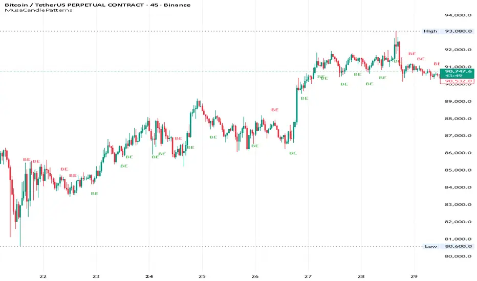
Bitcoin Cycle History Visualization [SwissAlgo]BTC 4-Year Cycle Tops & Bottoms
Historical visualization of Bitcoin's market cycles from 2010 to present, with projections based on weighted averages of past performance.
-----------------------------------------------------------------
CALCULATION METHODOLOGY
Why Bottom-to-Bottom Cycle Measurement?
This indicator defines cycles as bottom-to-bottom periods. This is one of several valid approaches to Bitcoin cycle analysis:
- Focuses on market behavior (price bottoms) rather than supply schedule events (halving-to-halving)
- Bottoms may offer good reference points for some analytical purposes
- Tops tend to be extended periods that are harder to define precisely
- Aligns with how some traditional asset cycles are measured and the timing observed in the broader "risk-on" assets category
- Halving events are shown separately (yellow backgrounds) for reference
- Neither halving-based nor bottom-based measurement is inherently superior
Different analysts prefer different cycle definitions based on their analytical goals. This approach prioritizes observable market turning points.
Cycle Date Definitions
- Approximate monthly ranges used for each event (e.g., Nov 2022 bottom = Nov 1-30, 2022)
- Cycle 1: Jul 2010 bottom → Jun 2011 top → Nov 2011 bottom
- Cycle 2: Nov 2011 bottom → Dec 2013 top → Jan 2015 bottom
- Cycle 3: Jan 2015 bottom → Dec 2017 top → Dec 2018 bottom
- Cycle 4: Dec 2018 bottom → Nov 2021 top → Nov 2022 bottom
- Future cycles will be added as new top/bottom dates become firm
Duration Calculations
- Days = timestamp difference converted to days (milliseconds ÷ 86,400,000)
- Bottom → Top: days from cycle bottom to peak
- Top → Bottom: days from peak to next cycle bottom
- Bottom → Bottom: full cycle duration (sum of above)
Price Change Calculations
- % Change = ((New Price - Old Price) / Old Price) × 100
- Example: $200 → $19,700 = ((19,700 - 200) / 200) × 100 = 9,750% gain
- Approximate historical prices used (rounded to significant figures)
Weighted Average Formula
Recent cycles weighted more heavily to reflect the evolved market structure:
- Cycle 1 (2010-2011): EXCLUDED (too early-stage, tiny market cap)
- Cycle 2 (2011-2015): Weight = 1x
- Cycle 3 (2015-2018): Weight = 3x
- Cycle 4 (2018-2022): Weight = 5x
Formula: Weighted Avg = (C2×1 + C3×3 + C4×5) / (1+3+5)
Example for Bottom→Top days: (761×1 + 1065×3 + 1066×5) / 9 = 1,032 days
Projection Method
- Projected Top Date = Nov 2022 bottom + weighted avg Bottom→Top days
- Projected Bottom Date = Nov 2022 bottom + weighted avg Bottom→Bottom days
- Current days elapsed compared to weighted averages
- Warning symbol (⚠) shown when the current cycle exceeds the historical average
Technical Implementation
- Historical cycle dates are hardcoded (not algorithmically detected)
- Dates represent approximate monthly ranges for each event
- The indicator will be updated as the Cycle 5 top and bottom dates become confirmed
- Updates require manual code maintenance - not automatic
- Users should verify they're using the latest version for current cycle data
-----------------------------------------------------------------
FEATURES
- Background highlights for historical tops (red), bottoms (green), and halving events (yellow)
- Data table showing cycle durations and price changes
- Visual cycle boundary boxes with subtle coloring
- Projected timeframes displayed as dashed vertical lines
- Toggle on/off for each visual element
- Customizable background colors
-----------------------------------------------------------------
DISPLAY SETTINGS
- Show/hide cycle tops, bottoms, halvings, data table, and cycle boxes
- Customizable background colors for each event type
- Clean, institutional-grade visual design suitable for analysis
UPDATES & MAINTENANCE
This indicator is maintained as new cycle events occur. When Cycle 5's top and bottom are confirmed with sufficient time elapsed, the code and projections will be updated accordingly. Check for the latest version periodically.
OPEN SOURCE
Code available for review, modification, and improvement. Educational transparency is prioritized.
-----------------------------------------------------------------
IMPORTANT LIMITATIONS
⚠ EXTREMELY SMALL SAMPLE SIZE
Based on only 4 complete cycles (2011-2022). In statistical analysis, this is insufficient for reliable predictions.
⚠ CHANGED MARKET STRUCTURE
Bitcoin's market has fundamentally evolved since early cycles:
- 2010-2015: Tiny market cap, retail-only, unregulated
- 2024-2025: Institutional adoption, spot ETFs, regulatory frameworks, macro correlation
The environment that created past patterns no longer exists in the same form.
⚠ NO PREDICTIVE GUARANTEE
Historical patterns can and do break. Market cycles are not laws of physics. Past performance does not guarantee future results. The next cycle may not follow historical averages.
⚠ LENGTHENING CYCLE THEORY
Some analysts believe cycles are extending over time (diminishing returns, maturing market). If true, simple averaging underestimates future cycle lengths.
⚠ SELF-FULFILLING PROPHECY RISK
The halving narrative may be partially circular - it works because people believe it works. Sufficient changes in market structure or participant behavior can invalidate the pattern.
⚠ APPROXIMATE DATA
Historical prices rounded to significant figures. Exact bottom/top dates vary by exchange. Month-long ranges are used for simplicity.
EDUCATIONAL USE ONLY
This indicator is designed for historical analysis and understanding Bitcoin's past behavior. It is NOT:
- Trading advice or financial recommendations
- A guarantee or prediction of future price movements
- Suitable as a sole basis for investment decisions
- A replacement for fundamental or technical analysis
The projections show "what if the pattern continues exactly" - not "what will happen."
Always conduct independent research, understand the risks, and consult qualified financial advisors before making investment decisions. Only invest what you can afford to lose.

Bitcoin Polynomial Regression ModelThis is the main version of the script. Click here for the Oscillator part of the script.
💡Why this model was created:
One of the key issues with most existing models, including our own Bitcoin Log Growth Curve Model , is that they often fail to realistically account for diminishing returns. As a result, they may present overly optimistic bull cycle targets (hence, we introduced alternative settings in our previous Bitcoin Log Growth Curve Model).
This new model however, has been built from the ground up with a primary focus on incorporating the principle of diminishing returns. It directly responds to this concept, which has been briefly explored here .
📉The theory of diminishing returns:
This theory suggests that as each four-year market cycle unfolds, volatility gradually decreases, leading to more tempered price movements. It also implies that the price increase from one cycle peak to the next will decrease over time as the asset matures. The same pattern applies to cycle lows and the relationship between tops and bottoms. In essence, these price movements are interconnected and should generally follow a consistent pattern. We believe this model provides a more realistic outlook on bull and bear market cycles.
To better understand this theory, the relationships between cycle tops and bottoms are outlined below:https://www.tradingview.com/x/7Hldzsf2/
🔧Creation of the model:
For those interested in how this model was created, the process is explained here. Otherwise, feel free to skip this section.
This model is based on two separate cubic polynomial regression lines. One for the top price trend and another for the bottom. Both follow the general cubic polynomial function:
ax^3 +bx^2 + cx + d.
In this equation, x represents the weekly bar index minus an offset, while a, b, c, and d are determined through polynomial regression analysis. The input (x, y) values used for the polynomial regression analysis are as follows:
Top regression line (x, y) values:
113, 18.6
240, 1004
451, 19128
655, 65502
Bottom regression line (x, y) values:
103, 2.5
267, 211
471, 3193
676, 16255
The values above correspond to historical Bitcoin cycle tops and bottoms, where x is the weekly bar index and y is the weekly closing price of Bitcoin. The best fit is determined using metrics such as R-squared values, residual error analysis, and visual inspection. While the exact details of this evaluation are beyond the scope of this post, the following optimal parameters were found:
Top regression line parameter values:
a: 0.000202798
b: 0.0872922
c: -30.88805
d: 1827.14113
Bottom regression line parameter values:
a: 0.000138314
b: -0.0768236
c: 13.90555
d: -765.8892
📊Polynomial Regression Oscillator:
This publication also includes the oscillator version of the this model which is displayed at the bottom of the screen. The oscillator applies a logarithmic transformation to the price and the regression lines using the formula log10(x) .
The log-transformed price is then normalized using min-max normalization relative to the log-transformed top and bottom regression line with the formula:
normalized price = log(close) - log(bottom regression line) / log(top regression line) - log(bottom regression line)
This transformation results in a price value between 0 and 1 between both the regression lines. The Oscillator version can be found here.
🔍Interpretation of the Model:
In general, the red area represents a caution zone, as historically, the price has often been near its cycle market top within this range. On the other hand, the green area is considered an area of opportunity, as historically, it has corresponded to the market bottom.
The top regression line serves as a signal for the absolute market cycle peak, while the bottom regression line indicates the absolute market cycle bottom.
Additionally, this model provides a predicted range for Bitcoin's future price movements, which can be used to make extrapolated predictions. We will explore this further below.
🔮Future Predictions:
Finally, let's discuss what this model actually predicts for the potential upcoming market cycle top and the corresponding market cycle bottom. In our previous post here , a cycle interval analysis was performed to predict a likely time window for the next cycle top and bottom:
In the image, it is predicted that the next top-to-top cycle interval will be 208 weeks, which translates to November 3rd, 2025. It is also predicted that the bottom-to-top cycle interval will be 152 weeks, which corresponds to October 13th, 2025. On the macro level, these two dates align quite well. For our prediction, we take the average of these two dates: October 24th 2025. This will be our target date for the bull cycle top.
Now, let's do the same for the upcoming cycle bottom. The bottom-to-bottom cycle interval is predicted to be 205 weeks, which translates to October 19th, 2026, and the top-to-bottom cycle interval is predicted to be 259 weeks, which corresponds to October 26th, 2026. We then take the average of these two dates, predicting a bear cycle bottom date target of October 19th, 2026.
Now that we have our predicted top and bottom cycle date targets, we can simply reference these two dates to our model, giving us the Bitcoin top price prediction in the range of 152,000 in Q4 2025 and a subsequent bottom price prediction in the range of 46,500 in Q4 2026.
For those interested in understanding what this specifically means for the predicted diminishing return top and bottom cycle values, the image below displays these predicted values. The new values are highlighted in yellow:
And of course, keep in mind that these targets are just rough estimates. While we've done our best to estimate these targets through a data-driven approach, markets will always remain unpredictable in nature. What are your targets? Feel free to share them in the comment section below.

Bitcoin Polynomial Regression OscillatorThis is the oscillator version of the script. Click here for the other part of the script.
💡Why this model was created:
One of the key issues with most existing models, including our own Bitcoin Log Growth Curve Model , is that they often fail to realistically account for diminishing returns. As a result, they may present overly optimistic bull cycle targets (hence, we introduced alternative settings in our previous Bitcoin Log Growth Curve Model).
This new model however, has been built from the ground up with a primary focus on incorporating the principle of diminishing returns. It directly responds to this concept, which has been briefly explored here .
📉The theory of diminishing returns:
This theory suggests that as each four-year market cycle unfolds, volatility gradually decreases, leading to more tempered price movements. It also implies that the price increase from one cycle peak to the next will decrease over time as the asset matures. The same pattern applies to cycle lows and the relationship between tops and bottoms. In essence, these price movements are interconnected and should generally follow a consistent pattern. We believe this model provides a more realistic outlook on bull and bear market cycles.
To better understand this theory, the relationships between cycle tops and bottoms are outlined below:https://www.tradingview.com/x/7Hldzsf2/
🔧Creation of the model:
For those interested in how this model was created, the process is explained here. Otherwise, feel free to skip this section.
This model is based on two separate cubic polynomial regression lines. One for the top price trend and another for the bottom. Both follow the general cubic polynomial function:
ax^3 +bx^2 + cx + d.
In this equation, x represents the weekly bar index minus an offset, while a, b, c, and d are determined through polynomial regression analysis. The input (x, y) values used for the polynomial regression analysis are as follows:
Top regression line (x, y) values:
113, 18.6
240, 1004
451, 19128
655, 65502
Bottom regression line (x, y) values:
103, 2.5
267, 211
471, 3193
676, 16255
The values above correspond to historical Bitcoin cycle tops and bottoms, where x is the weekly bar index and y is the weekly closing price of Bitcoin. The best fit is determined using metrics such as R-squared values, residual error analysis, and visual inspection. While the exact details of this evaluation are beyond the scope of this post, the following optimal parameters were found:
Top regression line parameter values:
a: 0.000202798
b: 0.0872922
c: -30.88805
d: 1827.14113
Bottom regression line parameter values:
a: 0.000138314
b: -0.0768236
c: 13.90555
d: -765.8892
📊Polynomial Regression Oscillator:
This publication also includes the oscillator version of the this model which is displayed at the bottom of the screen. The oscillator applies a logarithmic transformation to the price and the regression lines using the formula log10(x) .
The log-transformed price is then normalized using min-max normalization relative to the log-transformed top and bottom regression line with the formula:
normalized price = log(close) - log(bottom regression line) / log(top regression line) - log(bottom regression line)
This transformation results in a price value between 0 and 1 between both the regression lines.
🔍Interpretation of the Model:
In general, the red area represents a caution zone, as historically, the price has often been near its cycle market top within this range. On the other hand, the green area is considered an area of opportunity, as historically, it has corresponded to the market bottom.
The top regression line serves as a signal for the absolute market cycle peak, while the bottom regression line indicates the absolute market cycle bottom.
Additionally, this model provides a predicted range for Bitcoin's future price movements, which can be used to make extrapolated predictions. We will explore this further below.
🔮Future Predictions:
Finally, let's discuss what this model actually predicts for the potential upcoming market cycle top and the corresponding market cycle bottom. In our previous post here , a cycle interval analysis was performed to predict a likely time window for the next cycle top and bottom:
In the image, it is predicted that the next top-to-top cycle interval will be 208 weeks, which translates to November 3rd, 2025. It is also predicted that the bottom-to-top cycle interval will be 152 weeks, which corresponds to October 13th, 2025. On the macro level, these two dates align quite well. For our prediction, we take the average of these two dates: October 24th 2025. This will be our target date for the bull cycle top.
Now, let's do the same for the upcoming cycle bottom. The bottom-to-bottom cycle interval is predicted to be 205 weeks, which translates to October 19th, 2026, and the top-to-bottom cycle interval is predicted to be 259 weeks, which corresponds to October 26th, 2026. We then take the average of these two dates, predicting a bear cycle bottom date target of October 19th, 2026.
Now that we have our predicted top and bottom cycle date targets, we can simply reference these two dates to our model, giving us the Bitcoin top price prediction in the range of 152,000 in Q4 2025 and a subsequent bottom price prediction in the range of 46,500 in Q4 2026.
For those interested in understanding what this specifically means for the predicted diminishing return top and bottom cycle values, the image below displays these predicted values. The new values are highlighted in yellow:
And of course, keep in mind that these targets are just rough estimates. While we've done our best to estimate these targets through a data-driven approach, markets will always remain unpredictable in nature. What are your targets? Feel free to share them in the comment section below.