Regression Fit Bollinger Bands [Spiritualhealer117]This indicator is best suited for mean reversion trading, shorting at the upper band and buying at the lower band, but it can be used in all the same ways as a standard bollinger band.
It differs from a normal bollinger band because it is centered around the linear regression line, as opposed to the moving average line, and uses the linear regression of the standard deviation as opposed to the standard deviation.
This script was an experiment with the new vertical gradient fill feature.
Regression

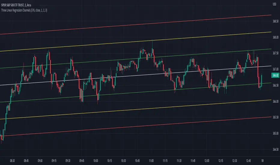
Three Linear Regression ChannelsPlot three linear regression channels using alexgrover 's Computing The Linear Regression Using The WMA And SMA indicator for the linear regression calculations.
Settings
Length : Number of inputs to be used
Source : Source input of the indicator
Midline Colour : The colour of the midline
Channel One, Two, and Three Multiplicative Factor : Multiplication factor for the RMSE, determine the distance between the upper and lower level
Channel One, Two, and Three Colour : The channel's lines colour
Usage
For usage details, please refer to alexgrover 's Computing The Linear Regression Using The WMA And SMA indicator.
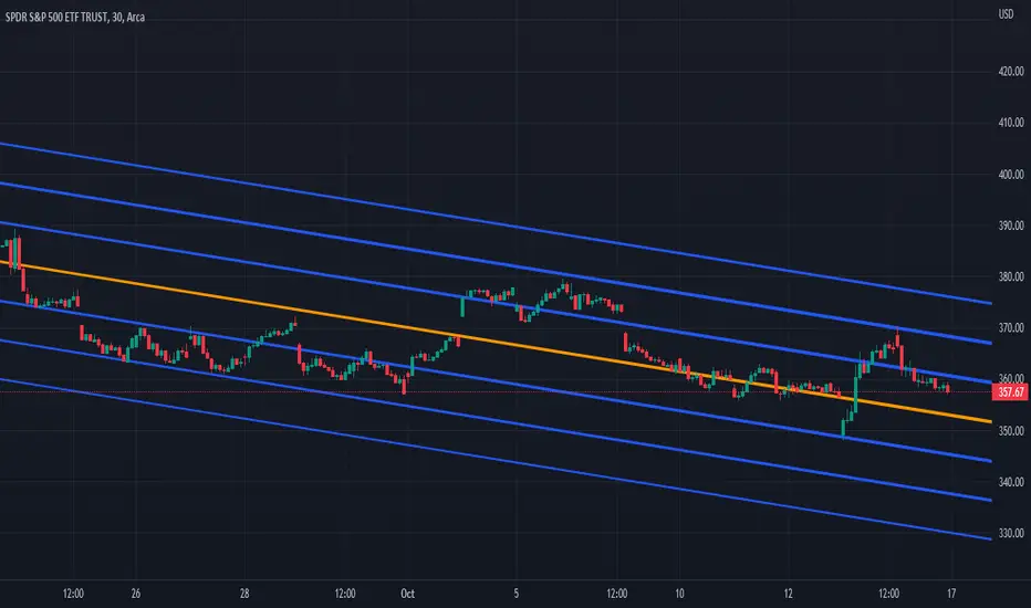
Multi-Optimized Linear Regression ChannelA take on alexgrover 's Optimized Linear Regression Channel script which allows users to apply multiple linear regression channel with unique multiplicative factors.
Multiplicative Factors
Adjust the amount of channels and multiplicative factors of existing or additional channels using the "Mults" input.
An input of "1" creates a single linear regression channel with the multiplicative factor of one.
An input of "4" creates a single linear regression channel with the multiplicative factor of four.
An input of "1,4" creates two linear regression channels with multiplicative factors of one and four.
An input of "1,2,3" creates three linear regression channels with multiplicative factors of one, two, and three.
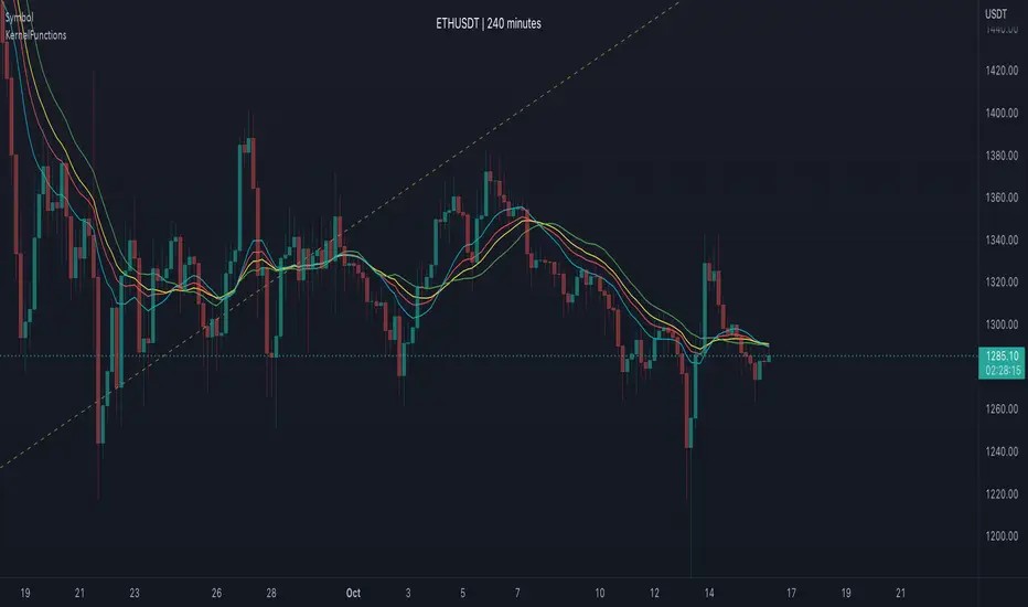
KernelFunctionsLibrary "KernelFunctions"
This library provides non-repainting kernel functions for Nadaraya-Watson estimator implementations. This allows for easy substitution/comparison of different kernel functions for one another in indicators. Furthermore, kernels can easily be combined with other kernels to create newer, more customized kernels. Compared to Moving Averages (which are really just simple kernels themselves), these kernel functions are more adaptive and afford the user an unprecedented degree of customization and flexibility.
rationalQuadratic(_src, _lookback, _relativeWeight, _startAtBar)
Rational Quadratic Kernel - An infinite sum of Gaussian Kernels of different length scales.
Parameters:
_src : The source series.
_lookback : The number of bars used for the estimation. This is a sliding value that represents the most recent historical bars.
_relativeWeight : Relative weighting of time frames. Smaller values result in a more stretched-out curve, and larger values will result in a more wiggly curve. As this value approaches zero, the longer time frames will exert more influence on the estimation. As this value approaches infinity, the behavior of the Rational Quadratic Kernel will become identical to the Gaussian kernel.
_startAtBar : Bar index on which to start regression. The first bars of a chart are often highly volatile, and omitting these initial bars often leads to a better overall fit.
Returns: yhat The estimated values according to the Rational Quadratic Kernel.
gaussian(_src, _lookback, _startAtBar)
Gaussian Kernel - A weighted average of the source series. The weights are determined by the Radial Basis Function (RBF).
Parameters:
_src : The source series.
_lookback : The number of bars used for the estimation. This is a sliding value that represents the most recent historical bars.
_startAtBar : Bar index on which to start regression. The first bars of a chart are often highly volatile, and omitting these initial bars often leads to a better overall fit.
Returns: yhat The estimated values according to the Gaussian Kernel.
periodic(_src, _lookback, _period, _startAtBar)
Periodic Kernel - The periodic kernel (derived by David Mackay) allows one to model functions that repeat themselves exactly.
Parameters:
_src : The source series.
_lookback : The number of bars used for the estimation. This is a sliding value that represents the most recent historical bars.
_period : The distance between repititions of the function.
_startAtBar : Bar index on which to start regression. The first bars of a chart are often highly volatile, and omitting these initial bars often leads to a better overall fit.
Returns: yhat The estimated values according to the Periodic Kernel.
locallyPeriodic(_src, _lookback, _period, _startAtBar)
Locally Periodic Kernel - The locally periodic kernel is a periodic function that slowly varies with time. It is the product of the Periodic Kernel and the Gaussian Kernel.
Parameters:
_src : The source series.
_lookback : The number of bars used for the estimation. This is a sliding value that represents the most recent historical bars.
_period : The distance between repititions of the function.
_startAtBar : Bar index on which to start regression. The first bars of a chart are often highly volatile, and omitting these initial bars often leads to a better overall fit.
Returns: yhat The estimated values according to the Locally Periodic Kernel.
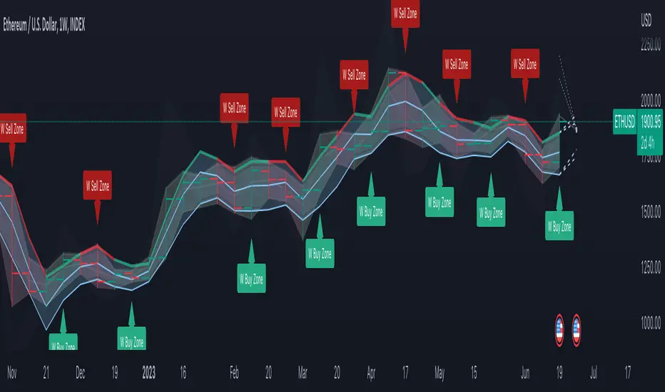
DB Change Forecast ProDB Change Forecast Pro
What does the indicator do?
The DB Change Forecast Pro is a unique indicator that uses price change on HLC3 to detect buy and sell periods along with plotting a linear regression price channel with oversold and undersold zones. It also has a linear regression change forecast mode to optionally project market direction.
Change is calculated by taking a two-bar change of HLC3 and dividing that by the price or, optionally, a fixed divisor.
A fast-moving change cloud is then calculated and displayed as the "regular version" plot (shown in light gray). When the cloud bottom is above low, a buy zone is detected. When the cloud top is below the high, a sell zone is detected.
The linear regression price channel is calculated similarly but using a much slower change rate. The linear regression price channel shows reasonable high, low and HLC3 ranges. At the bar's opening, the channel will be more compact and come fairly accurate about 1/4 into the bar timeframe.
The change forecasted price is projected on the right side of the current bar to indicate the current timeframe direction. Please note this forecasting feature is shown in orange when it's early in the timeframe and gray when the timeframe is more likely to produce an accurate direction forecast for the upcoming bar.
You can use these projected dashed lines to see possible market movements for the Current bar and possible market direction for the next bar. Kindly note these projects change; they should be used to understand possible extreme highs/lows for the current bar or market direction.
The indicator includes an optional change forecast projection feature hidden by default. It will project the market forecast channel with an offset of 1. The forecast is defaulted to an offset of 1 to show market direction. However, you can modify to zero the offset to show the current bar forecast and forecast history.
How should this indicator be used?
First, very important,
1. Settings > Set Symbol to Desired
2. Settings > Set High Timeframe to "Chart"
3. Settings > Ensure "Use price as divisor" is checked.
It's recommended to use this indicator in higher timeframes. Buy and sell signals are displayed in real-time. However, waiting until 1/4 to 1/2 into the current bar is recommended before taking action, and change can happen.
The buy/sell signals (zones) provide recommendations on playing a long vs. a short. When in a buy sone, only play longs. When in a sell zone, only play shorts.
Then use the linear regression price channel oversold and undersold zones to optionally open and close positions within the buy/sell zones.
For example, consider opening a long in a buy zone when the linear regression price channel shows undersold. Then consider closing the long when the price moves into the linear regression oversold or higher. Then repeat as long as it's in the buy zone. Then vice versa for sell zones and shorting.
At basic design, buy in the buy zone, sell or short in the sell zone. If you are up for higher trading frequencies, use the linear regression price channel as described in the example above.
Please note, as, with all indicators, you may need to adjust to fit the indicator to your symbol and desired timeframe.
This is only an example of use. Please use this indicator as your own risk and after doing your due diligence.
Does the indicator include any alerts?
Yes,
"DB CFHLC3: Signal BUY" - Is triggered when a buy signal is fired.
"DB CFHLC3: Signal SELL" - Is triggered when a sell signal is fired.
"DB CFHLC3: Zone BUY" - Is triggered when a buy zone is detected.
"DB CFHLC3: Zeon SELL" - Is triggered when a sell zone is detected.
"DB CFHLC3: Oversold SELL" - Is triggered when the price exceeds the oversold level.
"DB CFHLC3: Undersold BUY" - Is triggered when the price goes below the undersold level.
Any other tips?
Once you have configured the indicator for your symbol and chart timeframe. Meaning the plots are displayed over the price. Check out larger timeframes such as W, 2W, 3W, 4W, M, and 4M. It works wonderfully for showing market lows and highs for long-term investing too!
Another, tip is to combine it with your favorite indicator, such as TTM Squeeze or MACD for confirmation purposes. You may be surprised how fast the indicator shows market direction changes on higher timeframes.
You can just as easily use a high timeframe such as D, 2D, or 3D for day trading due to how the linear price channel works.
Why am I not selling this indicator?
I would like to bless the TradingView community, and I enjoy publishing custom indicators.
If you enjoy this indicator, please consider leaving a thumbs up or a comment for others to know about your experience or recommendations.
Enjoy!
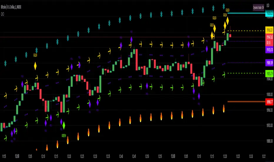
Quantitative Kernel DelimiterQuantitative Kernel Delimiter QKD - aka "Fire and ICE" - is a six-level multiple Kernel regression estimator with cross-timeframe semi-coordinated delimiters (bands) enabled by mathematical validation to our own Kernel regression code with historical Kernel formulas having custom variable bandwidths , mults , and window width – all achieving an advanced alerting system and directional price-action pointers for Novice, Intermediate and Advanced Traders within the TradingView Graphical User Interface.
In the course of our work, we have found that such six delimiters are ideal for generating signals of varying strengths.
99.9% of observations should be in our delimiters' range:
Kernel regression is a nonparametric smoothing method for data modeling.
Kernel regression of statistics was derived independently by Nadaraya and Watson in 1964 with a mathematical foundation given by Parzen’s earlier work on kernel density estimation.
If you are interested in reading more about the mathematical basis of this method from which our code is derived, you can follow these scholarly links:
Expert Trading Systems: Modeling Financial Markets with Kernel Regression
Estimation of the bandwidth parameter in Nadaraya-Watson
Adaptive optimal kernel density estimation for directional data
How kernel regression differs from the other Moving Averages?
In most MA's data points in the specified lookback window are weighted equally. In contrast, the Gaussian Kernel function used in this indicator assigns a higher weight to data points that are closer to the current point. This means that the indicator will react more quickly to changes in the market.
Regression method from which our code is derived is a widely known formula that is laid out in many sources, we used this source:
Kernel regression estimation
Kernel
During the regression counting process, a `kernel function` is used, which is traditionally chosen from a wide variety of symmetric functions.
In this indicator, we use the Gaussian density of statistics as the kernel function.
The Gaussian Kernel is one of the most commonly used Kernel functions and is used extensively in many Machine Learning algorithms due to its general applicability across a wide variety of datasets.
The kernel regression averages all the data contained within the range of the kernel function.
The effective range of the kernel function is defined by its window width .
Kernel Delimiters (Bands / Levels)
This indicator has 6 tailored price range* delimiters:
Cold / Fire - the furthest delimiters. In a range market when the price enters the cold/fire zones it is assumed that it has deviated strongly from the average and there is a high probability that it will immediately return to the average, or at least into the underlying zone, also in a trending market it signals a change in trend.
ALERT: the indicator performs best during relatively sideways price action within an established range. The trader must check higher timeframes during hits on the extreme Cold or Fire delimiter bands as a break in the lower, or even higher timeframe price range may result in a need to reset the regression calculation once price velocity calms down after a major move allowing the indicator to best function again. The reset will be done automatically by the indicator’s code. The indicator is not intended for use with unusually aggressive pricing behavior. Always beware of extreme market conditions. The indicator is intended as an ordinary range trading tool.
Gold / Green - we call it the middle ground / golden mean / happy medium zone. When the price comes out here but the momentum is not enough to get to the higher zone we consider it a good signal.
Pro - most often we receive signals in this area. We call it the professional zone because it is literally the zone for professional traders who know what they are dealing with.
*NOTE: the indicator is intended to be used as a range trading tool, and does not protect against total BREAKS from one Range to a new Range, wherein the bands reset for the trader.
Alerts / Labels
We have spent a lot of time implementing and testing signal labels* and alerts**.
Now you have access to an advanced alert system.
*NOTE: DUE TO the ongoing regression calculations performed by our code, the trader will note that a label may change color at a later point in time, or even soon after the hit on the quantitative delimiter band in question. This is a process that was reviewed and is favored to achieve visual clarity over historical accuracy for the trader. Real-time trading hits of price line to band, along with alerts generated, remain accurate. We look forward to receiving feedback on this issue from the end users. Additional revisions by our team on this matter are anticipated if a harmony between visual clarity and historical accuracy is not satisfied.
**NOTE: Smaller and especially micro timeframes will result in more repeated alerts given the tight proximity with price vis-à-vis the quantitative delimiter. Larger timeframes tend to eliminate any issue with repeated alerts aside from obvious re-contacting of the quantitative delimiter by the active price line.
You can turn off alerts you don't need in the indicator settings.
All alerts are set with one click.
Themes
Different people like different things, which is why we decided to make several visual design themes so you can choose what suits you.
Themes will continue to evolve over time.
Pro Theme:
Modern Theme:
How to remove colored text labels next to price scale to maximize screen space on mobile:
Go to General Chart Settings :
Click on “SCALES”
Un select “Indicators and financial name.”
Dynamic Mode
Projection of Indicator bands on history is subject to repainting due to its regressive calculation nature. Be cautious: old signals are drawn once at the first loading of the chart and by default (to speed up the start-up time of the indicator) correspond to the current regression levels. All labels remain in their places as the chart progresses. Also new, real-time labels appear on the chart, and do not disappear. In order to display the old signals on the chart as they were at the time of their appearance, uncheck the "History labels transition" in the indicator settings (it may increase the initial loading time of the chart but will give you an opportunity to check the alerts you received before and may also be useful for visual backtesting).
Because of the very nature of modeling financial markets (i.e., thousands of data records and perhaps hundreds of candidate predictors), the need for computational speed is paramount.
The use of kernel regression in data modeling for the types of problems associated with financial markets requires careful consideration of computational time.
Once we acknowledge that the order of the data is important, then the choice of the learning-data-set becomes crucial. The time dimension introduces another level of complexity to the analysis: how much importance do we attach to recent data records as opposed to earlier records? Is there a simple way to take this effect into consideration? Common sense leads us to the basic conclusion that if we are to predict a value of Y at a given time, we should only use learning data from an earlier time. But this procedure tends to be overly restrictive. This problem has a simple solution: All that one must do is to make the learning data set dynamic . In other words, once a record has been tested, it is then available for updating the learning data set prior to testing the next record. The analyst can allow the learning data set to grow, or, alternatively, for each record added, the earliest remaining record in the learning set can be discarded. These two alternatives have led us to the necessity of using moving window option and adding a disclaimer that dynamic mode is enabled.
This indicator will be updated frequently based on community feedback see the Author’s instructions below to get instant access
―――――――――――――――――――――
Liability Disclaimer
Never fully rely on one indicator as you trade. Successful trading may require an orchestral mindset and harmonіc blend of trading tools, know-how, and devices. VIP Trader . com is not responsible for any damages or losses incurred by use or misused of this indicator. Neither this description above, nor the indicator, is intended to be used as financial advisory tool, nor to be used without proper education or training in the field of trading.
SUPER GCOV5 MAPSCALP > MAPPING & SCALPING SUPER GCOV5 MAPSCALP indicator is built specifically for mapping/prediction measurement and fast trading i.e. scalping/intraday in the commodity market or cryptos market. It uses an indicator instrument consisting of ATR TRAILING STOP (ATR), EXPONENTIAL MOVING AVERAGE, PIVOT POINT, FIBONACCI KEY LEVEL, and LINEAR REGRESSION CHANNEL(LRC).
Rebuild of Instrument & Parameter
This indicator is also an upgraded instrument that is sourced from the previous indicator-FUTURES SCALPV2.This R&D of course makes trading activities more effective, and dynamic to increase the confidence of traders in current trading activities. The indicator has been upgraded in terms of parameters as well as additional instruments. Among them are;
1. ATR Trailing Stop
2. ATR BUY/SELL signal
3. Exponential Moving Average(EMA) – fastMA/slowMA Length
5. Breakout/breakdown signal
6. Pivot low/high level
7. Fibonacci extends & retracement
8. Linear Regression Channel(LRC)
9. Alert condition ( a dozen alerts )
> The best timeframe for entry is 3 minutes for FCPO and 15 minutes for other futures & cryptos.
> The best timeframe mapping/prediction is 1 hour & 4 hours.
>The candle/bars have been colored to make it easier for traders to see the price trends whether in bullish or bearish conditions.
Easier SOP of ENTRIES/POSITIONING:
1. entry by signal BUY/SELL after signal bar ( 2nd bar) for confirmation.
2. The best entries BUY at support(pivot low-Blue line) after price rebound then signal appears. The best buy also when the price is at lower
low pivot + fibo support level + lower trendline(LRC) + and the price went rebound.
3. The best entries SELL at resistance(pivot high-red line) after price pullback then signal appears.
The best buy also when the price is at a higher high pivot + fibo resistance level + upper trendline LRC + and the price went pullback.
4. Profit-taking areas are usually measured by support and resistance levels. Please refer to the bold line( support & resistance), fibo key level,
and trendline.
*To avoid false signals/wrong positions, you can use the EMA line as a guide and follow the trends, which are the buying weight when the price is above the 20/50 ema, and the selling weight when the price is below the 20/50 ema. EMA can be reset on the input setting.
STEPS of MAPPING/PROJECTION:
1. Use a bigger timeframe such as 4 hours or 1 hour
2. Use LRC to identify buy/sell weights when the price makes a zig-zag patent
3. Use monthly and weekly fibo levels to know support and resistance. This fibo is very important to see if the price will make an extension or
retracement based on the regression channel earlier. So here we can evaluate which area to buy/sell/take-profit/exit and the reversal of a
market price.
You can also create an ALERT CONDITION to help you get a reminder of signals and price trend changes
The original instrument has been retained but changed in terms of display & facelift features.
Hopefully, the new one will assist you in making analysis and strategy of trading activities successfully.
THIS IS NOT A BUY/SELL CALL, ONLY STUDY IDEAS AND ANALYSIS BASED ON MEASUREMENT TOOLS FOR EDUCATION AND GUIDANCE PURPOSES.PLEASE TAKE AT YOUR OWN RISK.

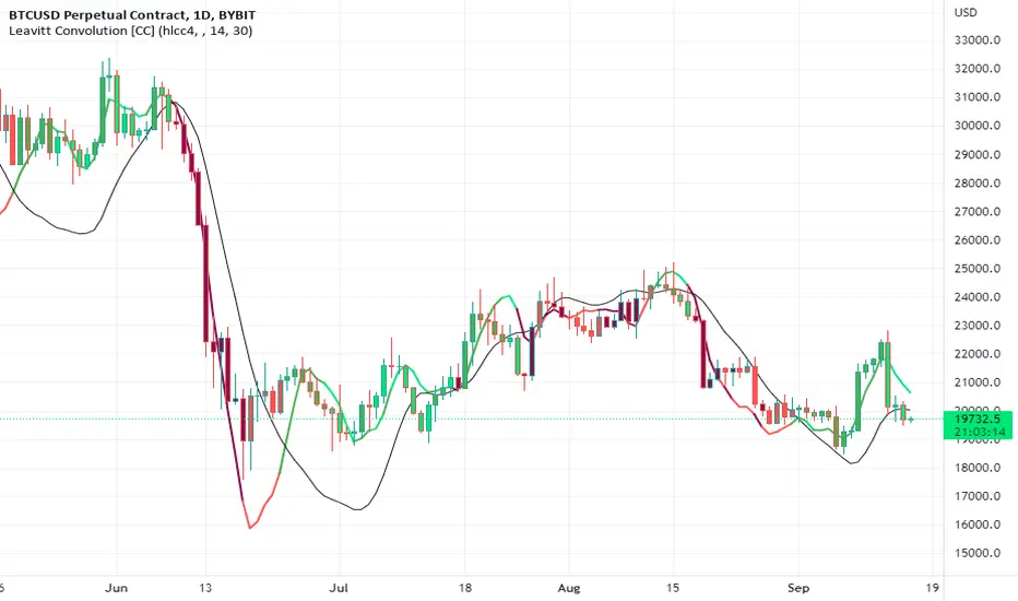
Leavitt Convolution [CC]The Leavitt Convolution indicator was created by Jay Leavitt (Stocks and Commodities Oct 2019, page 11), who is most well known for creating the Volume-Weighted Average Price indicator. This indicator is very similar to my Leavitt Projection script and I forgot to mention that both of these indicators are actually predictive moving averages. The Leavitt Convolution indicator doubles down on this idea by creating a prediction of the Leavitt Projection which is another prediction for the next bar. Obviously this means that it isn't always correct in its predictions but it does a very good job at predicting big trend changes before they happen. The recommended strategy for how to trade with these indicators is to plot a fast version and a slow version and go long when the fast version crosses over the slow version or to go short when the fast version crosses under the slow version. I have color coded the lines to turn light green for a normal buy signal or dark green for a strong buy signal and light red for a normal sell signal, and dark red for a strong sell signal.
This is another indicator in a series that I'm publishing to fulfill a special request from @ashok1961 so let me know if you ever have any special requests for me.
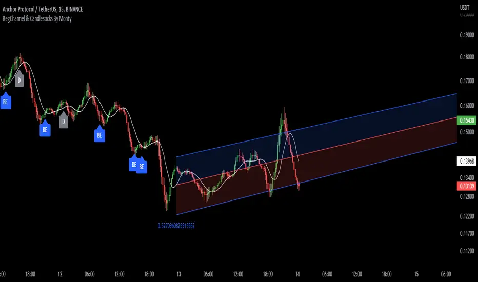
Regression Channel, Candles and Candlestick Patterns by MontyRegression Candles by ugurvu
Regression Channel by Tradingview
All Candlestick Patterns By Tradingview
This script was combined for a friend of mine who needed this.
This Script has regression candles by ugurvu, Regression channel and Candlestick patterns by tradingview.
The intention was to fuse these together so more information can be processed on the cost of a single indicator.
Standard Deviation Channel V.1Standard Deviation channel For TradingView V.1
Many thanks to and Made with help from @rumpypumpydumpy
█ - How to add the indicator-
You can “Boost” the tool if you like it, then scroll down on this page to "Add to favorite indicators" so it will be saved in your favorites. Easiest way to add to chart past that is simply copy the indicators name, Navigate to a chart, then paste the indicators name into your chart's "Indicators" tab. It should then be immediately added to the current chart. If your display is not large enough, when you first add your channel,, you may realize that you see labels appear, but no channel. Simply scroll backwards in time until the chart loads. TradingView needs to be able to see the data you would like the channel to read in order to plot and display correctly. This is a simple one or two mouse wheel scroll and it will appear.
You may notice a compression of price scale. IF this happens simply right click your right price axis, a menu will appear, select “Scale price chart only”, and "Auto (fits data to screen) This will release the scale compression and let you view the channel and price normally. Once your Channel is added, loaded, and ready to go, you can proceed to settings. In the top left corner of your main chart there will be a Indicator title, hover that and click on the gear icon to access the channels custom settings. You can also double click any of the active plots from the channel or averages on the chart, and gain access to the settings panel through that.
█ OVERVIEW
Settings explained -
Inputs and color choices
You can think of the settings panel as 3 separate sections.
First - Look and feel- You will have your Channels visual inputs, Simple Yes or No check boxes on whether you would like to display the visual items listed. You can choose to display the channel in a multitude of ways, with or without half deviations, with no 2nd, 3rd, or 4th deviations. This first section is your quick access control panel to the visual feel and display of the channel and its items.
Then below that you will see quick access color presets for each deviation and half deviations. You can choose to leave these as is, or you can choose custom colors per your preference.
The positive and negative Second deviations (+/-2std) are colored by positive and negative slope of channel. This will help to show overall trend, whether up or down, positive or negative. User can change the positive and negative slope colors if they would like.
Second, - Time and Regression - Next as you scroll down the settings panel you will encounter the Time and regression settings. In order for the channel to match the channel used widely in TOS, we had to Preset the look back lengths into the code because on Tradingview we have an “Continuous left edge of the chart”. We needed to tell the channel how far to look back and start calculating. The frame work for this time logic came initially from the channel that was developed years back by @corgalicious, We then took that time logic and re-worked it in order to fit the parameters that the widely used and popular TOS channel has.
Above the time frame length back inputs you will find a dropdown menu "Regression method type". This will offer different methods of regression and calculating the standard deviation from the center linear regression line. It is preset to “Population standard deviation” which will mimic the widely used TOS channel. There is also a choice for “Regression method standard error, or RMSE. This is a similar regression style, but will result in a tighter fitting, smaller deviation measurement and channel all around. As well as a multitude of other regression styles thanks to the genius of @rumpypumpydumpy
All the time presets were carefully chosen based off Pre set time frames TOS offers for their widely used Standard deviation channel, and time frames I had noted as widely used. You as the user can change those look back windows if you prefer through the input length settings. I recommend using the stock settings in most scenarios. Trading view has a 5000 bar look back limit, so we have implemented “Max lookbacks” inside the code to avoid any user error or confusion. The standard error of the sample mean is an estimate of how far the sample mean is likely to be from the population mean, whereas the standard deviation of the sample is the degree to which individuals within the sample differ from the sample mean. For longer time frames and sample sets I tend to use Population Standard Dev setting. For smaller sample sets I will go with Linreg RMSE setting. This is a personal preference. It is encouraged to try all of them and see what fits your trading style the best.
If the user would like to use a "Max bar lookback and plot the maximum allowed length on the current time frame, Simply select, "Use the full range of data allowed in max bars back for calculation?" This will automatically search back on the current time frame and plot the channel 4999 bars back. User will have to SCROLL BACK in order to fully load the channel into view. Again, Tradingview needs to see the candles you would like to plot on.
Third, - Finally at the bottom of the settings I have included Exponential moving average clouds. These are NOT enabled by default. If the user would like them enabled simply check "show momentum average clouds" and "Show Candle EMA". These are Multiple time frame moving average clouds consisting of 72/89 length 3, and 5min exponential moving averages. I use these to simply show the front or back side of a move and to find if trend is strong or weakening. These are not always needed so they are turned off by default.
█ CONCEPTS
Reversion and Repulsion-
You will find that the channel linear regression trend line has two characteristic's, Reversion to the mean, and Repulsion away from the mean. Price either seeks to aggressively return to the mean when it has exited a normal distribution, or price seeks to aggressively move away from the mean in times of momentum. Most seek to participate in the move through MAJOR WHOLE deviation levels in one scenario or the other.
The idea behind using a Standard deviation channel is to see extension and find where in the move we are. Are you extended out to 3 or 4 deviation's up or down? If so, you could start to think about reversion back to the mean. Have you had a violent move down to -3 or -4 deviations in a sell off? Maybe look at reversion back up toward the mean off a whole deviation break. Have you broken out of a normal distribution at +1 deviation and are building trend? maybe seek to join trend.
I have found most success by using a Split screen style layout. On the left chart most will have a 1min intraday channel showing, and on the left chart a 4hr channel showing. The idea is to mark your longer time frame deviations onto your intraday time frame, and use the intraday Channel to guide you through the higher time framed move. The move through +/- 1 deviation is a high momentum area in most names as price either seeks to return to the mean, or move strongly away from the mean.
█ Time periods
The channel has pre determined lookback presets for each major time frame. These have been preset in the code to mimic the widely used channel in TOS to the best of our ability.
Preset timeframe lookbacks include.
//intraday shorter time frames. 1/2min with 2day lookbacks
'1D-1Min' - Default= 2D, minval=1, maxval=5
'1D-2Min' - Default= 2D, minval=1, maxval=7
//intraday shorter time frames. 3/5min with 5day lookbacks. User can set shorter or longer if they choose, up to a 5000k bar look back depending on their Data tier level, Basic, Pro, Pro+, Premium etc.
'5D-3Min' - Default= 5D, minval=1, maxval=7
'5D-5Min' - Default= 5D, minval=1, maxval=20
// larger intraday time frames, 10/15min with 5day look backs.
'5D-10Min' - Default= 5D, minval=1, maxval=20
'5D-15Min' - Default= 5D, minval=1, maxval=60
// "Swing style time frames" 30/60 min with 10 and 20 day look back.
'10D-30Min' - Default= 10D, minval=1, maxval=60
'20D-1Hr' - Default= 20D, minval=1, maxval=90
//longer lookbacks for larger time frames using day lookback with the exception of week/month
'90D-2Hr' - Default = 90D, minval=1, maxval=180
'4h ' - Default = 180D,minval=1, maxval=4999
'6h' - Default = 36D, minval=1, maxval=252
'5Yr-W' - Default = 260W,minval=1, maxval=260
'1Yr-1D' - Default = 252D,minval=1, maxval=4999
'1Yr-1W' - Default = 52W, minval=1, maxval=480
'5Yr-1M' - Default = 60W, minval=1, maxval=480
█ Minimum Window Size
Note that on each time frame you MUST quickly scroll out to the first bar that the channel should start calculating on in order for the channel to populate on longer time frame series. This is under construction and as soon as there is a fix or other way around this, it will be addressed.
█ NOTES
Enjoy!
In the end I encourage any who tries the Channel to really sit down and spend some time playing around with the settings in order to find out how they like the Channel set up. I usually run the default settings on a intraday 5min chart, and then another instance of the study on a 4 hour chart. That way I can see granular intraday levels, and macro long term levels in the same view. See what fit's you the best, and how you like to trade. Most of all ENJOY!
Good luck -
JMF.
IMPORTANT INFO-
As always, the creator of this code is NOT a licensed investment advisor. No output of this tool is to be taken as investment advice or a recommendation to buy or sell any security.
Trading is risky, any one using this tool acknowledges they CAN LOSE some if not all of their initial investment even with this tool enabled.
User assumes ALL RESPONSIBILITY when using this tool in their technical analysis. There is NO GUARANTEE THAT THE USE OF THIS TOOL WILL RESULT IN PROFIT Use at your own risk.
RSI + MA, LinReg, ZZ (HH HL LH LL), Div, Ichi, MACD and TSI HistRelative Strength Index with Moving Average, Linear Regression, Zig Zag (Highs and Lows), Divergence, Ichimoku Cloud, Moving Average Convergence Divergence and True Strength Index Histogram
This script is based on zdmre's RSI script, I revamped a lot of things and added a few indicators from ParkF's RSI script.
Disable Labels in the Style tab and the histogram if you don't enlarge the indicator and it seems too small.
Look to buy in the oversold area and bounce of the support of the linear regression.
Look to sell in the overbought area and bounce of the resistance of the linear regression.
Look for retracement to the moving average or horizontal lines, and divergences for potential reversal.
RSI
The Relative Strength Index (RSI) is a well versed momentum based oscillator which is used to measure the speed (velocity) as well as the change (magnitude) of directional price movements.
Moving Average
Moving Average (MA) is a good way to gauge momentum as well as to confirm trends, and define areas of support and resistance.
Linear Regression
The Linear Regression indicator visualizes the general price trend of a specific part of the chart based on the Linear Regression calculation.
Zig Zag (Highs and Lows)
The Zig Zag indicator is used to identify price trends, and in doing so plots points on the chart to mark whenever prices reverse by a larger percentage point than a predetermined variable or marker.
Divergence
The divergence indicator warns traders and technical analysts of changes in a price trend, oftentimes that it is weakening or changing direction.
Ichimoku Cloud
The Ichimoku Cloud is a package of multiple technical indicators that signal support, resistance, market trend, and market momentum.
MACD and TSI Histogram
MACD can be used to identify aspects of a security's overall trend.
The True Strength Index indicator is a momentum oscillator designed to detect, confirm or visualize the strength of a trend.

R2-Adaptive RegressionOVERVIEW
This is an implementation of alexgrover's R2-Adaptive Regression optimized for the latest version of TradingView.
Full details on the indicator are on alexgrover's page here:

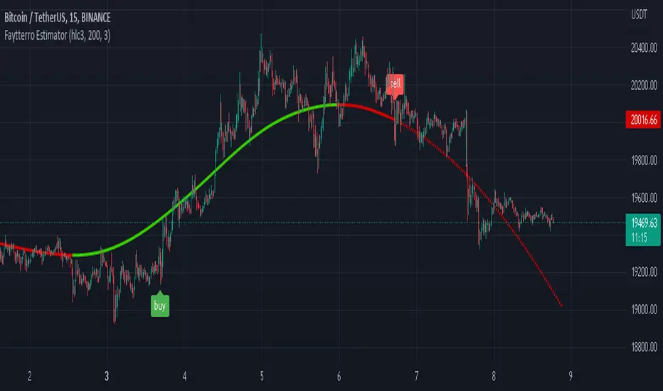
Faytterro EstimatorWhat is Faytterro Estimator?
This indicator is an advanced moving average.
What it does?
This indicator is both a moving average and at the same time, it predicts the future values that the price may take based on the values it has taken before.
How it does it?
takes the weighted average of data of the selected length (reducing the weight from the middle to the ends). then draws a parabola through the last three values, creating a predicted line.
How to use it?
it is simple to use. You can use it both as a regression to review past prices, and to predict the future value of a price. uptrends are in green and downtrends are in red. color change indicates a possible trend change.
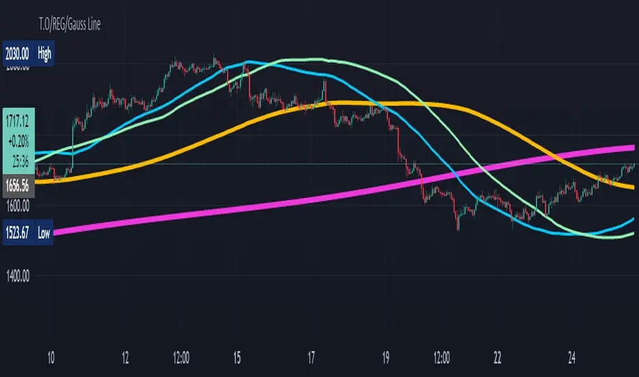
T.O/REG/Gauss LineHi Dear Traders/Dealers!
I present you here 3 lines that I developed myself base on statistical issues.
+Reg. Line
+Gauss Line
+T.O Line
-Reg. Line based on linear regression of previous inputs to make an average value.
-Gauss Line based on Gaussian mean value, Standard Deviation and it uses previous inputs to make an average value.
-T.O Line based on Gaussian and RMA methods generate an average value.
Hopefully useful for you!
Best regards and happy trading
Shakib
Polynomial Regression Derivatives [Loxx]Polynomial Regression Derivatives is an indicator that explores the different derivatives of polynomial position. This indicator also includes a signal line. In a later release, alerts with signal markings will be added.
Polynomial Derivatives are as follows
1rst Derivative - Velocity: Velocity is the directional speed of a object in motion as an indication of its rate of change in position as observed from a particular frame of reference and as measured by a particular standard of time (e.g. 60 km/h northbound). Velocity is a fundamental concept in kinematics, the branch of classical mechanics that describes the motion of bodies.
2nd Derivative - Acceleration: In mechanics, acceleration is the rate of change of the velocity of an object with respect to time. Accelerations are vector quantities (in that they have magnitude and direction). The orientation of an object's acceleration is given by the orientation of the net force acting on that object.
3rd Derivative - Jerk: In physics, jerk or jolt is the rate at which an object's acceleration changes with respect to time. It is a vector quantity (having both magnitude and direction). Jerk is most commonly denoted by the symbol j and expressed in m/s3 (SI units) or standard gravities per second (g0/s).
4th Derivative - Snap: Snap, or jounce, is the fourth derivative of the position vector with respect to time, or the rate of change of the jerk with respect to time. Equivalently, it is the second derivative of acceleration or the third derivative of velocity.
5th Derivative - Crackle: The fifth derivative of the position vector with respect to time is sometimes referred to as crackle. It is the rate of change of snap with respect to time.
6nd Derivative - Pop: The sixth derivative of the position vector with respect to time is sometimes referred to as pop. It is the rate of change of crackle with respect to time.
Included:
Loxx's Expanded Source Types
Loxx's Moving Averages

Regression Channel Trend DetectionThis is a regression channel that uses ichimoku to determine trend. The sensitivity is customizable. The centerline will change color according to the trend detected by ichimoku, and each line can act as support/resistance. The bands of the channel also change colors according to how far price is getting away from them. If you notice in this example, the lower band is turning orange when the price is getting too far away from it, suggesting that it may have risen too fast and too soon. This is still in testing so feel free to comment with any suggestions or fixes.
Polynomial-Regression-Fitted RSI [Loxx]Polynomial-Regression-Fitted RSI is an RSI indicator that is calculated using Polynomial Regression Analysis. For this one, we're just smoothing the signal this time. And we're using an odd moving average to do so: the Sine Weighted Moving Average. The Sine Weighted Moving Average assigns the most weight at the middle of the data set. It does this by weighting from the first half of a Sine Wave Cycle and the most weighting is given to the data in the middle of that data set. The Sine WMA closely resembles the TMA (Triangular Moving Average). So we're trying to tease out some cycle information here as well, however, you can change this MA to whatever soothing method you wish. I may come back to this one and remove the point modifier and then add preliminary smoothing, but for now, just the signal gets the smoothing treatment.
What is Polynomial Regression?
In statistics, polynomial regression is a form of regression analysis in which the relationship between the independent variable x and the dependent variable y is modeled as an nth degree polynomial in x. Polynomial regression fits a nonlinear relationship between the value of x and the corresponding conditional mean of y, denoted E(y |x). Although polynomial regression fits a nonlinear model to the data, as a statistical estimation problem it is linear, in the sense that the regression function E(y | x) is linear in the unknown parameters that are estimated from the data. For this reason, polynomial regression is considered to be a special case of multiple linear regression .
Included
Alerts
Signals
Bar coloring
Loxx's Expanded Source Types
Loxx's Moving Averages
Other indicators in this series using Polynomial Regression Analysis.
Poly Cycle
PA-Adaptive Polynomial Regression Fitted Moving Average
Polynomial-Regression-Fitted Oscillator
Polynomial-Regression-Fitted Oscillator [Loxx]Polynomial-Regression-Fitted Oscillator is an oscillator that is calculated using Polynomial Regression Analysis. This is an extremely accurate and processor intensive oscillator.
What is Polynomial Regression?
In statistics, polynomial regression is a form of regression analysis in which the relationship between the independent variable x and the dependent variable y is modeled as an nth degree polynomial in x. Polynomial regression fits a nonlinear relationship between the value of x and the corresponding conditional mean of y, denoted E(y |x). Although polynomial regression fits a nonlinear model to the data, as a statistical estimation problem it is linear, in the sense that the regression function E(y | x) is linear in the unknown parameters that are estimated from the data. For this reason, polynomial regression is considered to be a special case of multiple linear regression .
Things to know
You can select from 33 source types
The source is smoothed before being injected into the Polynomial fitting algorithm, there are 35+ moving averages to choose from for smoothing
This indicator is very processor heavy. so it will take some time load on the chart. Ideally the period input should allow for values from 1 to 200 or more, but due to processing restraints on Trading View, the max value is 80.
Included
Alerts
Signals
Bar coloring
Other indicators in this series using Polynomial Regression Analysis.
Poly Cycle
PA-Adaptive Polynomial Regression Fitted Moving Average

TF Segmented Polynomial Regression [LuxAlgo]This indicator displays polynomial regression channels fitted using data within a user selected time interval.
The model is fitted using the same method described in our previous script:
Settings
Degree: Degree of the fitted polynomial
Width: Multiplicative factor of the model RMSE. Controls the width of the polynomial regression's channels
Timeframe: Fits the polynomial regression using data within the selected timeframe interval
Show fit for new bars: If selected, will fit the regression model for newly generated bars, else the previous fitted value is displayed.
Src: Input source
Usage
Segmented (or piecewise) models yield multiple fits by first partitioning the data into multiple intervals from specific partitioning conditions. In this script this partitioning condition is for a user selected timeframe to change.
Segmented models can be particularly pertinent for market prices, which often describes a series of local trends.
Segmented polynomial regressions can describe the nature of underlying trends in the price from their fit, such as if an underlying trend is more linear (trending) or constant (ranging), and if a trend is monotonic.
The above chart shows a monthly partitioning on SPX 15m, using a polynomial regression of degree 3. Channel extremities allows highlighting local tops/bottoms.
For real time applications users can choose to fit a current model to incoming price data using the Show fit for new bars settings.
Details
The script does not make use of line.new to display the segmented linear regressions, which allows showing a higher number of historical fits. Each channel extremity as well as the model fit is displayed from the plot function, as such user can more easily set alerts on them.
It is important to note that achieving this requires accessing future price data, as such this script is subject to lookahead bias, historical results differ from the results one could have obtained in real-time.

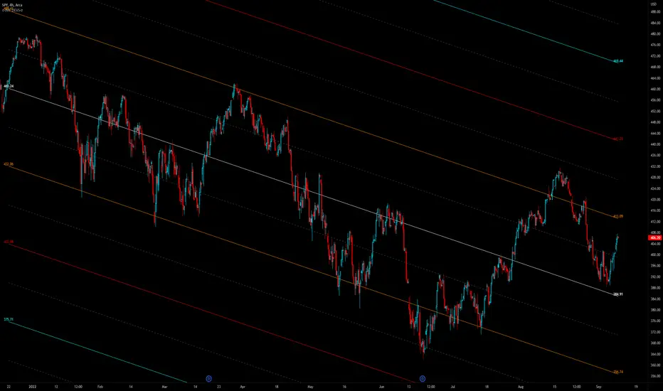
Regression Channel Alternative MTF█ OVERVIEW
This indicator displays 3 timeframes of parallel channel using linear regression calculation to assist manual drawing of chart patterns.
This indicator is not true Multi Timeframe (MTF) but considered as Alternative MTF which calculate 100 bars for Primary MTF, can be refer from provided line helper.
The timeframe scenarios are defined based on Position, Swing and Intraday Trader.
█ INSPIRATIONS
These timeframe scenarios are defined based on Harmonic Trading : Volume Three written by Scott M Carney.
By applying channel on each timeframe, MW or ABCD patterns can be easily identified manually.
This can also be applied on other chart patterns.
█ CREDITS
Scott M Carney, Harmonic Trading : Volume Three (Reaction vs. Reversal)
█ TIMEFRAME EXPLAINED
Higher / Distal : The (next) longer or larger comparative timeframe after primary pattern has been identified.
Primary / Clear : Timeframe that possess the clearest pattern structure.
Lower / Proximate : The (next) shorter timeframe after primary pattern has been identified.
Lowest : Check primary timeframe as main reference.
█ EXAMPLE OF USAGE / EXPLAINATION

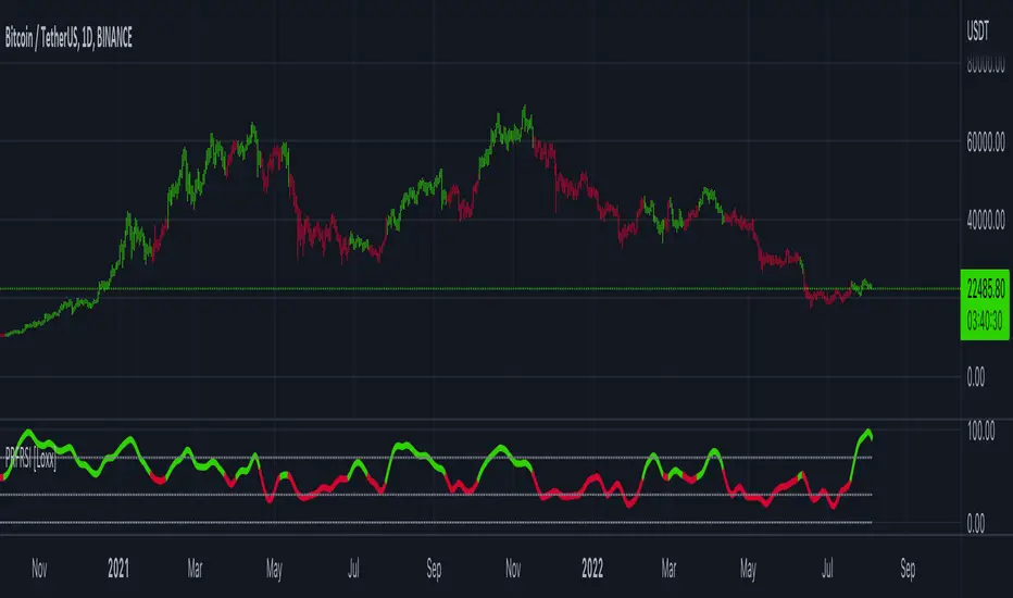
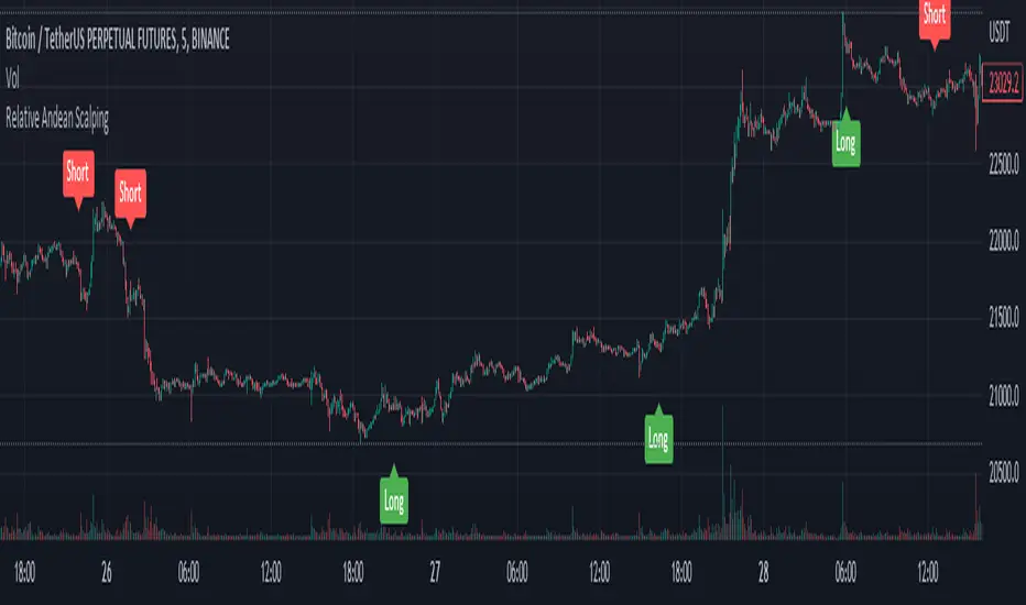
Relative Andean ScalpingThis is an experimental signal providing script for scalper that uses 2 of open source indicators.
First one provides the signals for us called Andean Oscillator by @alexgrover . We use it to create long signals when bull line crosses over signal line while being above the bear line. And reverse is true for shorts where bear line crosses over signal line while being above bull line.
Second one is used for filtering out low volatility areas thanks to great idea by @HeWhoMustNotBeNamed called Relative Bandwidth Filter . We use it to filter out signals and create signals only when the Relative Bandwith Line below middle line.
The default values for both indicators changed a bit, especially used linreg values to create relatively better signals. These can be changed in settings. Please be aware that i did not do extensive testing with this indicator in different market conditions so it should be used with caution.
Linear Regression ChannelsThese channels are generated from the current values of the linear regression channel indicator, the standard deviation is calculated based off of the RSI . This indicator gives an idea of when the linear regression model predicts a change in direction.
You are able to change the length of the linear regression model, as well as the size of the zone. A negative zone size will make the zone stretch away from the center, and a positive zone size will make it stretch towards the centerline.

Polynomial Regression Extrapolation [LuxAlgo]This indicator fits a polynomial with a user set degree to the price using least squares and then extrapolates the result.
Settings
Length: Number of most recent price observations used to fit the model.
Extrapolate: Extrapolation horizon
Degree: Degree of the fitted polynomial
Src: Input source
Lock Fit: By default the fit and extrapolated result will readjust to any new price observation, enabling this setting allow the model to ignore new price observations, and extend the extrapolation to the most recent bar.
Usage
Polynomial regression is commonly used when a relationship between two variables can be described by a polynomial.
In technical analysis polynomial regression is commonly used to estimate underlying trends in the price as well as obtaining support/resistances. One common example being the linear regression which can be described as polynomial regression of degree 1.
Using polynomial regression for extrapolation can be considered when we assume that the underlying trend of a certain asset follows polynomial of a certain degree and that this assumption hold true for time t+1...,t+n . This is rarely the case but it can be of interest to certain users performing longer term analysis of assets such as Bitcoin.
The selection of the polynomial degree can be done considering the underlying trend of the observations we are trying to fit. In practice, it is rare to go over a degree of 3, as higher degree would tend to highlight more noisy variations.
Using a polynomial of degree 1 will return a line, and as such can be considered when the underlying trend is linear, but one could improve the fit by using an higher degree.
The chart above fits a polynomial of degree 2, this can be used to model more parabolic observations. We can see in the chart above that this improves the fit.
In the chart above a polynomial of degree 6 is used, we can see how more variations are highlighted. The extrapolation of higher degree polynomials can eventually highlight future turning points due to the nature of the polynomial, however there are no guarantee that these will reflect exact future reversals.
Details
A polynomial regression model y(t) of degree p is described by:
y(t) = β(0) + β(1)x(t) + β(2)x(t)^2 + ... + β(p)x(t)^p
The vector coefficients β are obtained such that the sum of squared error between the observations and y(t) is minimized. This can be achieved through specific iterative algorithms or directly by solving the system of equations:
β(0) + β(1)x(0) + β(2)x(0)^2 + ... + β(p)x(0)^p = y(0)
β(0) + β(1)x(1) + β(2)x(1)^2 + ... + β(p)x(1)^p = y(1)
...
β(0) + β(1)x(t-1) + β(2)x(t-1)^2 + ... + β(p)x(t-1)^p = y(t-1)
Note that solving this system of equations for higher degrees p with high x values can drastically affect the accuracy of the results. One method to circumvent this can be to subtract x by its mean.