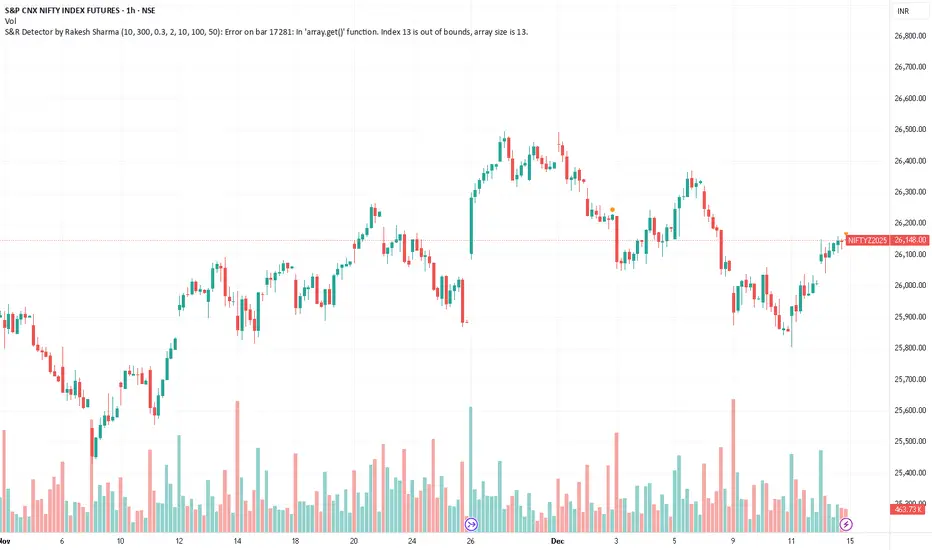
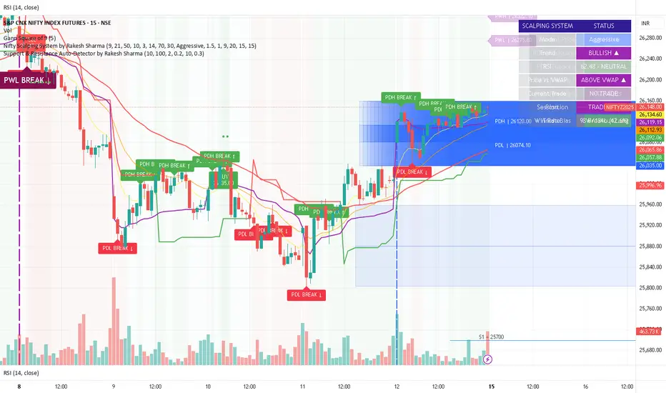
S&R Detector by Rakesh SharmaSupport & Resistance Auto-Detector
Automatically identifies key Support and Resistance levels with strength ratings
✨ Key Features:
🎯 Intelligent S/R Detection
Automatically finds Support and Resistance levels based on swing highs/lows
Shows strength rating (Very Strong, Strong, Medium, Weak)
Displays number of touches at each level
📅 Key Time-Based Levels
Previous Day High/Low (PDH/PDL) - Blue lines
Previous Week High/Low (PWH/PWL) - Purple lines
Optional Round Numbers for psychological levels
⚙️ Fully Customizable
Adjust sensitivity (5-20 pivot length)
Filter by minimum touches (1-10)
Control maximum levels displayed (3-20)
Optional S/R zones (shaded areas)
📊 Live Dashboard
Shows nearest Support/Resistance
Distance to key levels
Total S/R levels detected
🔔 Smart Alerts
PDH/PDL breakout signals
Visual markers on chart
Perfect for: Intraday traders, Swing traders, Price action analysis
Göstergeler ve stratejiler
S&R Detector by Rakesh Sharma📊 Support & Resistance Auto-Detector
Automatically identifies key Support and Resistance levels with strength ratings
✨ Key Features:
🎯 Intelligent S/R Detection
Automatically finds Support and Resistance levels based on swing highs/lows
Shows strength rating (Very Strong, Strong, Medium, Weak)
Displays number of touches at each level
📅 Key Time-Based Levels
Previous Day High/Low (PDH/PDL) - Blue lines
Previous Week High/Low (PWH/PWL) - Purple lines
Optional Round Numbers for psychological levels
⚙️ Fully Customizable
Adjust sensitivity (5-20 pivot length)
Filter by minimum touches (1-10)
Control maximum levels displayed (3-20)
Optional S/R zones (shaded areas)
📊 Live Dashboard
Shows nearest Support/Resistance
Distance to key levels
Total S/R levels detected
🔔 Smart Alerts
PDH/PDL breakout signals
Visual markers on chart
Perfect for: Intraday traders, Swing traders, Price action analysis

Ultimate Adaptive RSIUltimate Adaptive RSI
RSI That Adapts to Any Market
This isn't your grandpa's RSI. It dynamically adjusts its sensitivity based on market conditions—smoother in trends, responsive in ranges.
Traditional RSI fails in strong trends and changing volatility. UA-RSI fixes both by adapting its sensitivity in real-time, giving you reliable signals whether the market is trending, ranging, or transitioning between regimes.
How It Adapts:
Smart Pre-Smoothing: Uses Efficiency Ratio to detect trend strength and automatically lengthens/shortens its smoothing window.
Dominant Cycle Detection: Matches its internal period to the market's actual rhythm.
Dynamic Bands: RMS-based overbought/oversold levels that expand/contract with volatility.
Smoothing Stack: ALMA pre-smoothing → Ultimate Smoother → Jurik filter creates the cleanest RSI you've ever seen.
Trade Signals:
Buy: RSI crosses above lower band or midline + price confirms
Sell: RSI crosses below upper band or midline + price confirms
Bands expand in high volatility → wait for deeper extremes
Bands contract in low volatility → take earlier signals
Signal line for crossover entries
Adaptive smoothing = fewer false signals in trends
Day trading: Use 1.0 band multiplier
Swing trading: Use 1.2-1.5 multiplier
Ranging markets: Lower multiplier to 0.8
Trending markets: Raise multiplier to 1.5+
Bands widen in volatility = wait for deeper extremes
Bands tighten in calm markets = take earlier signals
Never trade RSI alone - always wait for price confirmation

S&R Detector by Rakesh SharmaSupport & Resistance Auto-Detector
Automatically identifies key Support and Resistance levels with strength ratings
✨ Key Features:
🎯 Intelligent S/R Detection
Automatically finds Support and Resistance levels based on swing highs/lows
Shows strength rating (Very Strong, Strong, Medium, Weak)
Displays number of touches at each level
📅 Key Time-Based Levels
Previous Day High/Low (PDH/PDL) - Blue lines
Previous Week High/Low (PWH/PWL) - Purple lines
Optional Round Numbers for psychological levels
⚙️ Fully Customizable
Adjust sensitivity (5-20 pivot length)
Filter by minimum touches (1-10)
Control maximum levels displayed (3-20)
Optional S/R zones (shaded areas)
📊 Live Dashboard
Shows nearest Support/Resistance
Distance to key levels
Total S/R levels detected
🔔 Smart Alerts
PDH/PDL breakout signals
Visual markers on chart
Perfect for: Intraday traders, Swing traders, Price action analysis

Ultimate Reversion BandsURB – The Smart Reversion Tool
URB Final filters out false breakouts using a real retest mechanism that most indicators miss. Instead of chasing wicks that fail immediately, it waits for price to confirm rejection by retesting the inner band—proving sellers/buyers are truly exhausted.
Eliminates fakeouts – The retest filter catches only genuine reversions
Triple confirmation – Wick + retest + optional volume/RSI filters
Clear visuals – Outer bands show extremes, inner bands show retest zones
Works on any timeframe – From scalping to swing trading
Perfect for traders tired of getting stopped out by false breakouts.
Core Construction:
Smart Dynamic Bands:
Basis = Weighted hybrid EMA of HLC3, SMA, and WMA
Outer Bands = Basis ± (ATR × Multiplier)
Inner Bands = Basis ± (ATR × Multiplier × 0.5) → The "retest zone"
The Unique Filter: The Real Retest
Step 1: Identify an extreme wick touching the outer band
Step 2: Wait 1-3 bars for price to return and touch the inner band
Why it works: Most false breakouts never retest. A genuine reversal shows seller/buyer exhaustion by allowing price to come back to the "halfway" level.
Optional Confirmations:
Volume surge filter (default ON)
RSI extremes filter (optional)
Each can be toggled ON/OFF
How to Use:
Watch for extreme wicks touching the red/lime outer bands
Wait for the retest – price must return to touch the inner band (dotted line) within 3 bars
Enter on confirmation with built-in volume/RSI filters
Set stops beyond the extreme wick

Capitulation Detector StrategyA multi-factor capitulation detector designed to identify exhaustion points in extended trends. It focuses on fading capitulation moves after multi-leg trends with extreme volume and price extension.
━━━━━━━━━━━━━━━━━━━━━━━━━━━━━━━━━━━━━━━━
THE CONCEPT
Capitulation occurs when the last holders give up — panic selling into lows or euphoric buying into highs. These moments create asymmetric opportunities because:
Sentiment becomes maximally skewed
Weak hands are flushed out
Price deviates far from equilibrium
The "fuel" for continuation is exhausted
━━━━━━━━━━━━━━━━━━━━━━━━━━━━━━━━━━━━━━━━
THE 6 FACTORS
Trend Persistence — Price stays on one side of 38 EMA for 12+ bars, confirming a sustained directional move
Acceleration — Price stays on one side of 5 EMA for 3+ bars, showing the move is accelerating into exhaustion
Volume Spike — Current bar volume ≥ 2x the 20-bar average
Body Expansion — Candle body ≥ 1.5x average, showing conviction/panic in the move
Extension — Price is 2+ ATR away from the 38 EMA, indicating overextension from equilibrium
Multi-Leg Structure — At least 3 consecutive lower lows (for longs) or higher highs (for shorts)
━━━━━━━━━━━━━━━━━━━━━━━━━━━━━━━━━━━━━━━━
SIGNAL LOGIC
Bullish Capitulation: 4+ factors align + price below 38 EMA + down candle + volume spike
Bearish Capitulation: 4+ factors align + price above 38 EMA + up candle + volume spike
The strategy enters counter-trend, fading the exhaustion move.
━━━━━━━━━━━━━━━━━━━━━━━━━━━━━━━━━━━━━━━━
EXIT OPTIONS
ATR-based stop loss (default: 2 ATR)
ATR-based take profit (default: 3 ATR)
Optional trailing stop
Time filter for session-specific trading
━━━━━━━━━━━━━━━━━━━━━━━━━━━━━━━━━━━━━━━━
BEST PRACTICES
Works best on liquid instruments with clean trends
More reliable after 3+ legs in the trend
Higher conviction when daily AND intraday timeframes align
"The bigger and more extended, the better"
Consider VWAP as additional confirmation (not coded here)
━━━━━━━━━━━━━━━━━━━━━━━━━━━━━━━━━━━━━━━━
SETTINGS GUIDE
Min Score: Increase for fewer, higher-quality signals
Volume Spike Multiplier: 2x; increase for stricter filter
Extension ATR: Higher values = more overextended setups only
Trend Bars Min: Higher values = longer established trends required
━━━━━━━━━━━━━━━━━━━━━━━━━━━━━━━━━━━━━━━━
ALERTS
Bullish Capitulation (potential long)
Bearish Capitulation (potential short)
━━━━━━━━━━━━━━━━━━━━━━━━━━━━━━━━━━━━━━━━
DISCLAIMER
This is a counter-trend strategy — inherently higher risk than trend-following. Always use proper position sizing and risk management. Backtest thoroughly on your specific instruments and timeframes.

VixTrixVixTrix - Because markets move in both directions.
VixTrix was born from a fundamental limitation in traditional volatility indicators: they only measure downside panic, completely missing the greed-driven extremes that form market tops.
How It Works:
Dual-Component Analysis:
vixBear = Panic selling intensity (distance from recent highs)
vixBull = FOMO buying intensity (distance from recent lows)
Oscillator = vixBear - vixBull = Net fear/greed imbalance
When the oscillator is positive, fear dominates (potential bottom forming). When negative, greed dominates (potential top forming).
Professional-Grade Filtering:
The magic happens with the symmetric RMS (Root Mean Square) bands. Unlike fixed percentage bands or standard deviation, RMS:
Creates mathematically symmetric positive/negative thresholds
Naturally adapts to changing volatility regimes
Provides statistical significance to extremes
VixTrix also adds selectable MA smoothing for the RMS calculation:
WMA (default): Balanced – middle-ground approach
VWMA: Volume-weighted – filters low-volume noise
EMA: Responsive – catches quick reversals
SMA: Stable – for swing trading
HMA: Fast and smooth – ideal for day trading
Signals require triple confirmation:
Statistical Extreme: Oscillator beyond RMS band
Price Action Confirmation: Correct candle color (bullish for bottoms, bearish for tops)
Momentum Continuation: Oscillator still moving toward extreme (exhaustion)
This multi-filter approach reduces premature entries and false signals while maintaining early positioning at potential reversal points.
Why This Matters for Your Trading:
In bull markets, traditional fear indicators sit near zero, giving no warning of impending tops.
VixTrix identifies when greed becomes excessive – when FOMO buying reaches statistical extremes that often precede corrections.
In range-bound markets, VixTrix excels at identifying overreactions in both directions, providing high-probability mean reversion opportunities.
During crashes, it captures the panic selling with the same precision as VixFix, but with better timing through its momentum confirmation.
VixTrix spots continuations through:
"No Signal" = Healthy Trend – Oscillator stays between RMS bands (no exhaustion)
Failed Extremes – Touches band but no triple confirmation = trend likely continues
Hidden Divergence – Price makes higher low while oscillator makes shallower low = uptrend continues
Controlled Emotions – Oscillator negative but not extreme in uptrends (greed present but not excessive)
Key Insight: When VixTrix doesn't give a signal during a pullback, institutions aren't panicking – they're just pausing before resuming the trend.
Green columns = Bullish exhaustion (potential bottoms)
Red columns = Bearish exhaustion (potential tops)
Golden RMS bands = Dynamic thresholds adapting to current volatility
Background highlights = Active signal conditions
The Result: A professional-grade oscillator that works in all market conditions – trending up, trending down, or ranging – by measuring the complete emotional spectrum driving price action.
Slope Failure (Momentum Stall) STRATEGY//======================================================================================
// SLOPE FAILURE (MOMENTUM STALL) STRATEGY
//--------------------------------------------------------------------------------------
// WHAT THIS STRATEGY DOES
// -----------------------
// This strategy trades **momentum failure**, not trend direction.
//
// Instead of predicting where price will go, it detects when **momentum can no longer
// continue in its current direction** and briefly fades that failure.
//
// Core idea:
// - Momentum expands → slope grows
// - Momentum stalls → slope collapses or flips
// - That stall represents **state transition**, not noise
//
// The system exploits these transitions repeatedly at short horizons.
//
//--------------------------------------------------------------------------------------
// HOW MOMENTUM IS MEASURED
// ------------------------
// 1. Source price (optionally smoothed)
// 2. First derivative (slope = price - price )
// 3. Optional smoothing of the slope itself
//
// The slope represents **instantaneous directional force**, not trend bias.
//
//--------------------------------------------------------------------------------------
// ENTRY LOGIC (SLOPE FAILURE)
// ---------------------------
// • Bull Slope Failure (SHORT):
// - Prior slope was sufficiently positive
// - Current slope collapses to zero or below
// → Upward momentum failed → enter SHORT
//
// • Bear Slope Failure (LONG):
// - Prior slope was sufficiently negative
// - Current slope rises to zero or above
// → Downward momentum failed → enter LONG
//
// Optional:
// - Minimum slope band can be enforced to avoid weak/noisy failures
//
//--------------------------------------------------------------------------------------
// EXIT LOGIC
// ----------
// Primary exits are **force-based**, not price-based:
//
// • Longest Slope Local Turn (optional):
// - Detects when the strongest slope in a recent window has occurred
// - Exits when momentum starts decaying from that extreme
//
// • Percent Stop Loss (optional):
// - Fixed % protection relative to entry price
//
// The strategy does NOT rely on profit targets.
// Winners are exited when **momentum decays**, not when price "looks good".
//
//--------------------------------------------------------------------------------------
// POSITION SIZING
// ---------------
// This strategy supports **percent-of-equity sizing**, computed dynamically:
//
// position size = (account equity × % allocation) / price
//
// This allows:
// - P&L to scale smoothly
// - Drawdowns to remain proportional
// - The same logic to work across symbols and account sizes
//
//--------------------------------------------------------------------------------------
// STRATEGY CHARACTERISTICS
// ------------------------
// • High trade count
// • Win rate near ~45–50%
// • Small, fast losers
// • Slightly larger winners
// • Very low drawdown
//
// This profile is intentionally designed for **scalability**, not prediction.
//
//--------------------------------------------------------------------------------------
// IMPORTANT NOTES
// ---------------
// • This is NOT a trend-following strategy
// • This is NOT a mean-reversion guess
// • This is a momentum **state-transition detector**
//
// The edge comes from structure + exits + sizing — not indicators.
//
//======================================================================================

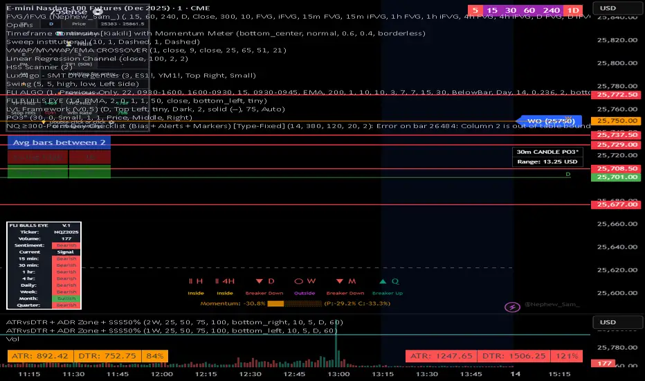
NQ 300+ Point Day Checklist (Bias + Alerts + Markers)This indicator helps identify high-range (≥300-point) days on Nasdaq-100 futures (NQ / MNQ) using a clear, rule-based checklist.
It evaluates volatility, compression, price displacement, prior-day structure, and overnight activity to generate a daily expansion score (0–6). Higher scores signal an increased likelihood of a strong trending or expansion day.
The script also provides:
Expansion probability levels (Normal / Watch / High-Prob)
Bullish, bearish, or neutral bias
On-chart markers and background highlights
Optional alerts for early awareness
Best used on the Daily timeframe to help traders focus on high-opportunity days and avoid overtrading during consolidation.
This is a context and probability tool — not a trade signal.
Vortex Imbalance DetectorVortex Imbalance Detector (VID)
Core Purpose:
To spot "fresh" institutional order flow entering the market, aiming to catch the early stage of a potential reversal driven by an imbalance between aggressive buyers and sellers.
It looks for moments when a surge in buying or selling pressure coincides with a sharp acceleration in price momentum at a market extreme.
The Vortex Imbalance Detector identifies high-probability reversal points by detecting simultaneous shifts in order flow (buy/sell pressure) and price momentum acceleration.
What It Does:
Order Flow Proxy: Creates a cumulative delta-like metric using price action (body vs. range) to estimate net buying or selling pressure.
Momentum Vortex: Calculates price acceleration (the rate of change of velocity) to gauge the force behind a move.
Imbalance Signal: Triggers when both conditions align:
Flow Flip: The order flow proxy crosses above/below zero with significant strength (exceeding a threshold).
Vortex Reversal: The momentum acceleration confirms the direction (positive for buys, negative for sells).
Price Extreme: The signal occurs at a recent low (for buys) or high (for sells).
Output:
Buy Signal (▲): A bullish order flow imbalance with upward momentum acceleration at a short-term low.
Sell Signal (▼): A bearish order flow imbalance with downward momentum acceleration at a short-term high.

CHOP-O-METER - Multi-Factor Choppiness DetectorA composite indicator that quantifies market choppiness using four independent measurements, helping you identify when to trade trends vs. when to sit out or fade moves.
━━━━━━━━━━━━━━━━━━━━━━━━━━━━━━━━━━━━━━━━
HOW IT WORKS
The Chop-O-Meter combines four normalized components (each scaled 0-100) into a single weighted score:
1. Price Efficiency (Kaufman-style)
Measures how efficiently price moved from point A to B. If price travels far but nets little distance, efficiency is low = high chop.
2. Direction Change Frequency
Counts how often price direction flips within the lookback period. More flips = more chop.
3. Mean Reversion Intensity
Tracks how often price crosses its moving average. Frequent crosses indicate a ranging, choppy market.
4. ATR Expansion Ratio
Compares the sum of individual bar ranges to the total period range. High ratio means lots of movement within a tight overall range = chop.
━━━━━━━━━━━━━━━━━━━━━━━━━━━━━━━━━━━━━━━━
READING THE INDICATOR
Above 65 (Red Zone): High chop — avoid trend-following, consider mean-reversion or staying flat
Below 35 (Green Zone): Trending — momentum strategies more likely to succeed
35-65 (Orange): Transitional/uncertain regime
━━━━━━━━━━━━━━━━━━━━━━━━━━━━━━━━━━━━━━━━
SIGNALS
🔻 Green triangle (top): Chop breaking down — potential trend starting
🔺 Red triangle (bottom): Trend exhausting — chop may be returning
━━━━━━━━━━━━━━━━━━━━━━━━━━━━━━━━━━━━━━━━
SETTINGS
Lookback Period: Number of bars to analyze (default 20)
Component Weights: Adjust influence of each factor
Thresholds: Customize high/low chop boundaries
Show Components: Toggle individual factor plots for debugging
━━━━━━━━━━━━━━━━━━━━━━━━━━━━━━━━━━━━━━━━
USE CASES
Filter out trend trades when chop score is high
Reduce position size in choppy regimes
Switch between mean-reversion and momentum strategies
Identify regime transitions early
━━━━━━━━━━━━━━━━━━━━━━━━━━━━━━━━━━━━━━━━
ALERTS INCLUDED
Entering High Chop
Entering Trend
Chop Breaking Down

CRUX-3 Macro Regime Index"CRUX-3 Macro Regime Index"
Description:
CRUX-3 Macro Regime Index is a higher-timeframe macro indicator designed to evaluate how crypto markets are performing relative to traditional equities. It compares Bitcoin, Ethereum, and the broader altcoin market (TOTAL3) against the S&P 500 using Z-score normalization to highlight periods of relative outperformance or underperformance.
The indicator incorporates liquidity-based regime detection using Bitcoin dominance and stablecoin dominance to classify market environments as Risk-On, BTC-Led, or Risk-Off. Background shading visually highlights these regimes, helping users identify broader macro conditions rather than short-term trade signals.
CRUX-3 is intended for macro context, regime awareness, and allocation bias decisions, not for precise trade entries or timing.
How to Use:
Weekly timeframe recommended for best results
Rising Z-scores indicate crypto outperforming equities
ETH/SPX typically acts as an early rotation signal
TOTAL3/SPX confirms broader altcoin participation
Regime shading reflects liquidity conditions, not price forecasts
Regime Definitions:
Risk-On: BTC dominance and stablecoin dominance declining
BTC-Led: BTC dominance strong while stablecoin dominance eases
Risk-Off: BTC dominance and stablecoin dominance rising
Notes:
Forward regime bands are statistical reference guides based on historical behavior
This indicator does not predict future prices or market direction
Best used alongside price charts and other macro tools
Disclaimer:
This indicator is for educational and informational purposes only. It does not constitute financial advice, investment advice, or trading recommendations.
Recommended Settings:
Timeframe: Weekly (1W)
Z-Score Lookback: 52
Forward Regime Bands: Enabled

Ahmed Gold Signals - 5M LIVE (Frequent)📈 Gold (XAUUSD) Trading Signals – Precision-Based Strategy
Our Gold signals are built on pure price action, not random indicators or guesswork.
🔍 How our signals are generated
We focus on:
🧲 Liquidity Sweeps
Identifying when price grabs stop-losses above highs or below lows and then reverses
📊 Clear trend direction using EMA 50 & EMA 200
✅ Strong confirmation candles after the sweep
🎯 Entries only in the direction of the trend to increase accuracy
🔵 BUY Signals
Bullish market structure
Price sweeps liquidity below recent lows
Strong bullish confirmation candle closes
➡️ High-probability BUY setup
🔴 SELL Signals
Bearish market structure
Price sweeps liquidity above recent highs
Strong bearish confirmation candle closes
➡️ High-probability SELL setup
⏱️ Timeframe
5-minute chart (5M)
Fast, precise signals ideal for scalping Gold
🛡️ Risk Management
Stop loss placed beyond the liquidity sweep
Clear take-profit targets
Risk-to-reward typically 1:2 or better
⚠️ Important Notes
We do not trade every move
We wait for confirmation
Quality over quantity — always

Support & Resistance Auto-Detector by Rakesh SharmaVersion 1.1 Update:
- Fixed: S/R lines now extend infinitely to the right
- Fixed: Lines move with chart when scrolling
- Added: Toggle to control line extension
- Improved: Better visibility across all timeframes
Al Brooks - Bar CountIndicator Purpose:
This indicator displays bar counts on the chart to help traders identify important time nodes and cycle transitions
Features smart session filtering with automatic futures/stock detection and appropriate trading session counting
Core Features:
Smart asset detection: Auto-detect futures and stocks
Session filter toggle: Choose all-day or session-specific counting
Auto timezone handling: Chicago time for futures, NY time for stocks
Flexible display control: Customizable display frequency and label size
Session Settings:
8:30-15:15 (CT) / Futures mode: Chicago time 8:30-15:15 (CT)
9:30-16:00 (ET) / Stock mode: New York time 9:30-16:00 (ET)
All-day mode: Count from first bar of the day
Timeframe Correspondence:
Multiples of 3: Correspond to 15-minute chart update cycles
Multiples of 12: Correspond to 1-hour chart update cycles
18: Key nodes, important time turning points

Al Brooks - EMA20Instead of simply fetching data from the 60-minute or 15-minute charts, this script mathematically simulates the internal logic of those EMAs directly on your current timeframe.
Just for fun.


Dynamic MAs Zscore | Lyro RSThe Dynamic MAs Zscore is an adaptive momentum and valuation oscillator built around advanced moving averages and statistical Z-Score normalization. By combining a wide selection of moving average types with dynamic deviation bands, this indicator delivers clear insights into trend strength , directional bias , and relative valuation — all in a clean, visually intuitive format.
━━━━━━━━━━━━━━━
Key Features
━━━━━━━━━━━━━━━
Dynamic Moving Average Engine
Applies one of 12 selectable moving average types (SMA, EMA, WMA, VWMA, HMA, ALMA, TEMA, etc.) to the chosen source. This allows fine-tuning between responsiveness and smoothness depending on market conditions.
Z-Score Normalization
Transforms the selected moving average into a standardized Z-Score:
(MA − mean) / standard deviation
This normalization makes momentum strength comparable across assets and timeframes.
Adaptive Deviation Bands
Upper and lower bands are derived from the rolling standard deviation of the Z-Score:
Custom band length
Independent positive and negative multipliers
These bands dynamically expand and contract with volatility.
Dual Signal Modes
Trend Mode – Focuses on directional continuation. Color changes and signals occur when Z-Score breaks above or below deviation bands.
Valuation Mode – Highlights relative overvaluation and undervaluation using a gradient color scale and predefined value zones.
Advanced Visual System
Includes bold layered plots, gradient fills, background shading, and candle/bar coloring to clearly reflect current market state.
Custom Color Palettes
Choose from multiple preset themes (Classic, Mystic, Accented, Royal) or define your own bullish and bearish colors.
━━━━━━━━━━━━━━━
How It Works
━━━━━━━━━━━━━━━
MA Calculation – The selected moving average type is applied to the chosen price source.
Z-Score Computation – The MA is normalized over a user-defined lookback period to quantify deviation from its mean.
Band Construction – Standard deviation of the Z-Score is calculated over the band length and scaled by positive/negative multipliers.
Mode-Dependent Logic
Trend Mode – Breaks above the upper band signal bullish momentum; breaks below the lower band signal bearish momentum.
Valuation Mode – A gradient reflects relative valuation from undervalued to overvalued, with background highlights at extreme Z-Score levels.
━━━━━━━━━━━━━━━
Signal Interpretation
━━━━━━━━━━━━━━━
Trend Confirmation
In Trend Mode, sustained moves beyond deviation bands indicate strong directional bias.
Momentum Strength
The distance of the Z-Score from zero reflects the intensity of trend momentum.
Relative Valuation
In Valuation Mode, deep negative Z-Scores suggest undervaluation, while high positive Z-Scores suggest overvaluation.
Visual Clarity
Bar and candle coloring aligned with oscillator state allows for rapid assessment of market conditions.
━━━━━━━━━━━━━━━
Customization
━━━━━━━━━━━━━━━
Adjust MA type and length to balance speed vs. smoothness.
Modify Z-Score length to control sensitivity.
Tune band length and multipliers for volatility adaptation.
Switch between Trend and Valuation modes depending on strategy.
Personalize visuals using preset or custom color palettes.
━━━━━━━━━━━━━━━
Alerts
━━━━━━━━━━━━━━━
Bullish condition when Z-Score > 0
Bearish condition when Z-Score < 0
Overvalued and undervalued valuation alerts
⚠️ Disclaimer
This indicator is intended for technical analysis and educational purposes only. It does not guarantee profitable outcomes and should be used alongside other tools, confirmation methods, and sound risk management. The author is not responsible for any financial decisions made using this indicator.

EMA Market Regime & Real-Time Candle Projection System📌 EMA Market Regime & Real-Time Candle Projection System
EMA Market Regime & Parabolic Projection is a real-time market structure system designed to anticipate candle behavior before it fully forms, by dynamically projecting price levels based on trend strength, acceleration, and market expansion.
Unlike traditional indicators that react after the candle closes, this system continuously adapts to live price data to provide early insight into bullish, bearish, parabolic, and exhaustion phases.
🔍 Core Concept
The system operates on four key dimensions:
Market Structure
Uses a fast and a slow EMA to determine the dominant market regime (bullish or bearish).
Directional Momentum
Measures EMA slope to confirm directional commitment.
Acceleration & Parabolic Detection
Identifies true parabolic movements through acceleration analysis, filtering out weak or range-bound price action.
Expansion Validation
Confirms that movements are supported by genuine market expansion, reducing false signals.
By combining these elements, the indicator projects a dynamic price level in real time, effectively drawing a forward-looking guide that adapts as each candle evolves.
🧠 Real-Time Candle Projection
The projected line represents a dynamic equilibrium level derived from EMA structure and acceleration.
This allows traders to:
Anticipate continuation vs exhaustion
Visualize momentum shifts before candle close
Read potential candle direction and strength in real time
The projection is non-repainting and updates tick-by-tick during the candle’s formation.
🎯 Market Regime Classification
The system automatically classifies the market into distinct states:
Bullish Trend – Positive structure with controlled momentum
Bearish Trend – Negative structure with controlled momentum
Parabolic Expansion – Accelerated trend with strong continuation potential
Parabolic Exhaustion – Loss of acceleration signaling potential reversal or pullback
Neutral / Range – Low momentum and low expansion (no-trade zone)
Each state is visually encoded using subtle, professional coloring, ensuring price candles always remain the primary focus.
🛡️ Professional-Grade Filters
Anti-range and anti-fake breakout filtering
Cooldown logic to prevent repetitive signals
Slope normalization relative to volatility
Designed to remain readable on M1–M5 scalping and higher timeframes
⚙️ Designed For
Scalping & Intraday Trading
Real-time decision-making
Trend continuation & exhaustion timing
Prop-firm and professional trading environments
This system is intended as a market structure and timing tool, not a signal spam indicator.
⚠️ Disclaimer
This indicator does not predict the future and does not provide guaranteed results. It is designed to assist discretionary traders by improving real-time market reading and execution timing.

Adaptive 2-Pole Trend Bands [supfabio]Adaptive 2-Pole Trend Bands is a volatility-aware trend filtering indicator designed to identify the dominant market direction while providing dynamic reference zones around price.
Instead of relying on traditional moving averages, this indicator uses a two-pole digital filter to smooth price action while maintaining responsiveness. Around this central trend line, a multi-band structure based on ATR is applied to help traders evaluate pullbacks, extensions, and potential exhaustion areas within a trend.
Core Concept
The indicator is built around three key ideas:
Digital Trend Filtering
Volatility-Adjusted Bands
Trend Persistence Measurement
These components work together to separate meaningful price movement from noise and to provide context for how far price has moved relative to recent volatility.
Two-Pole Trend Filter
At its core, the indicator uses a two-pole smoothing filter, which produces a cleaner trend curve than common moving averages.
Compared to standard averages, this approach:
Reduces market noise
Produces smoother transitions
Responds faster to genuine trend changes
Avoids excessive lag in trending markets
The result is a trend line that represents the structural direction of price, rather than short-term fluctuations.
Adaptive Multi-Band System
Around the central trend filter, the indicator plots four independent volatility-based bands, each derived from the Average True Range (ATR).
Each band represents a different degree of price extension:
Band 1: Shallow pullbacks and minor reactions
Band 2: Moderate extensions within a trend
Band 3: Strong directional moves
Band 4: Extreme extensions relative to recent volatility
Because the bands are ATR-based, they automatically adapt to changing market conditions, expanding during high volatility and contracting during calmer periods.
This makes the indicator suitable for both slow and fast markets without manual recalibration.
Trend State Detection
The color of the central filter dynamically reflects trend persistence, not just direction:
Sustained upward movement highlights bullish conditions
Sustained downward movement highlights bearish conditions
Transitional phases are visually distinct, helping identify regime changes
This logic is based on how long price has maintained directional behavior, reducing sensitivity to isolated candles or short-lived spikes.
Practical Applications
This indicator can be used as:
A trend filter for discretionary or systematic strategies
A context tool to evaluate pullbacks versus overextension
A risk reference to avoid entries in extreme price zones
A confirmation layer when combined with price action or momentum tools
It performs consistently across different asset classes, including futures, cryptocurrencies, forex, indices, and equities.
Configuration
Key parameters such as filter length, damping factor, and band multipliers are fully configurable, allowing traders to adapt the indicator to different timeframes and trading styles.
Important Notes
This indicator does not predict future price movement
It does not generate guaranteed buy or sell signals
Best results are achieved when used in combination with sound risk management and additional confirmation tools
Past behavior does not imply future performance
Disclaimer
This indicator is provided for educational and analytical purposes only and should not be considered financial advice.
Se quiser, posso:
Criar uma versão resumida para a primeira linha da publicação
Ajustar o texto para um tom mais técnico ou mais comercial
Traduzir para português mantendo o inglês como idioma principal
Revisar o título para SEO dentro da Biblioteca Pública

Ripster Clouds + Saty Pivot + RVOL + Trend1. Ripster EMA Clouds (local + higher timeframe)
Local timeframe (your chart TF):
Plots up to 5 EMA clouds (8/9, 5/12, 34/50, 72/89, 180/200 – configurable).
Each cloud is:
One short EMA and one long EMA.
A filled band between them.
Color logic:
Cloud is bullish when short EMA > long EMA (green/blue-ish tone).
Bearish when short EMA < long EMA (red/orange/pink tone).
You can choose:
EMA vs SMA,
Whether to show the lines,
Per-cloud toggles.
MTF Clouds:
Two higher-timeframe EMA clouds:
Cloud 1: 50/55
Cloud 2: 20/21
Computed on a higher TF (default D, but configurable).
Show as thin lines + transparent bands.
Used for:
Visual higher-TF trend,
Optional signal filter (MTF must agree for trades).
2. Saty Pivot Ribbon (time-warped EMAs)
This is basically your Saty Pivot Ribbon integrated:
Uses a “Time Warp” setting to overlay EMAs from another timeframe.
EMAs:
Fast, Pivot, Slow (defaults 8 / 21 / 34).
Clouds:
Fast cloud between fast & pivot EMAs.
Slow cloud between pivot & slow EMAs.
Bullish/bearish colors are distinct from Ripster colors.
Optional highlights:
Can highlight fast/pivot/slow lines separately.
Conviction EMAs:
13 and 48 EMAs (configurable).
When fast conviction EMA crosses over/under slow:
You get triangle arrows (bullish/bearish conviction).
Bias candles:
If enabled, candles are recolored based on:
Price vs Bias EMA,
Candle up/down/doji,
So you see bullish/bearish “bias” directly in candle colors.
3. DTR vs ATR panel (range vs average)
In a small table panel (bottom-center by default):
Computes higher-TF ATR (default 14, TF auto D/W/M, smoothing type selectable).
Measures current range (high–low) on that TF.
Displays:
DTR: X vs ATR: Y Z% (+/-Δ% vs prev)
Where:
Z% = current range / ATR * 100.
Δ% = change vs previous bar’s Z%.
Background color:
Greenish for low move (<≈70%),
Red for high move (≥≈90%),
Yellow in between,
Slightly dimmed when price is below bias EMA.
This tells you: “Is today an average, quiet, or explosive day compared to normal?”
4. SMA Divergence panel
Separate histogram & line panel:
Fast and slow SMAs (default 14 & 30).
Computes price divergence vs SMA in %:
% above/below slow SMA,
% above/below fast SMA.
Shows:
Slow SMA divergence as a semi-transparent column,
Fast SMA divergence as a solid column on top,
EMA of the slow divergence (trend line) colored:
Blue when rising,
Orange/red when falling.
Static upper/lower bands with fill, plus optional zero line.
This gives you a feel for how stretched price is vs its anchors.
5. RVOL table (relative volume)
Small 3×2 table (bottom-right by default):
Inputs:
Average length (default 50 bars),
Optionally show previous candle RVOL.
Calculates:
RVOL now = volume / avg(volume N bars) * 100,
RVOL prev,
RVOL momentum (now – prev) for data window only.
Table columns:
Candle Vol,
RVOL (Now),
RVOL (Prev).
Colors:
200% → “high RVOL” color,
100–200% → “medium RVOL” color,
<100% → “low RVOL” color,
Slightly dimmer if price is below bias EMA.
This is used both visually and optionally as a signal filter (e.g., only trade when RVOL ≥ threshold).
6. Trend Dashboard (Price + 34/50 + 5/12)
Top-right trend box with 3 rows:
Price Action row:
Uses either Bias EMA or custom EMA on close to say:
Bullish (close > trend EMA),
Bearish (close < trend EMA),
Flat.
Ripster 34/50 Cloud row:
Uses 34/50 EMAs: bullish if 34>50, bearish if 34<50.
Ripster 5/12 Cloud row:
Uses 5/12 EMAs: bullish if 5>12, bearish if 5<12.
Then it does a vote:
Counts bullish votes (Price, 34/50, 5/12),
Counts bearish votes,
Depending on mode:
Majority (2 of 3) or Strict (3 of 3).
Output:
Overall Bullish / Bearish / Sideways.
You also get an optional label on the chart like
Overall: Bullish trend with color, and an optional background tint (green/red for bull/bear).
7. VWAP + Buy/Sell Signals
VWAP is plotted as a white line.
Fast “trend” cloud mid: average of 5 & 12 EMAs.
Slow “trend” cloud mid: average of 34 & 50 EMAs.
Buy condition:
5/12 crosses above 34/50 (bullish cloud flip),
Price > VWAP,
Optional filter: MTF Cloud 1 bullish (50/55 on higher TF),
Optional filter: RVOL >= threshold.
Sell condition:
5/12 crosses below 34/50,
Price < VWAP,
Optional same filters but bearish.
When conditions are met:
Plots BUY triangle up below price (distinct teal/green tone).
Plots SELL triangle down above price (distinct magenta/orange tone).
Alert conditions are defined for:
BUY / SELL signals,
Overall Bullish / Bearish / Sideways change,
MTF Cloud 1 trend flips.
8. Data Window metrics
For easy backtesting / inspection via TradingView’s data window, it exposes:
DTR% (Current) and DTR% Momentum,
RVOL% (Now), RVOL% (Prev), RVOL% Momentum.
TL;DR – What does this script do for you?
It turns your chart into a multi-framework trend and momentum dashboard:
Ripster EMA clouds for short/medium trend & S/R.
Saty Ribbon for higher-TF pivot structure and conviction.
RVOL + DTR/ATR for context (is this a big and well-participated move?).
SMA divergence panel for overextension/stretch.
A compact trend table that tells you Price vs 34/50 vs 5/12 in one glance.
Buy/Sell markers + alerts when:
short-term Ripster trend (5/12) flips over/under medium (34/50),
price agrees with VWAP,
plus optional filters (MTF trend and / or RVOL).
Basically: it’s a trend + confirmation + context system wrapped into one indicator, with most knobs configurable in the settings.

Strategy with VWRSI and SAVE orders Long or Short or BothVWRSI is very powerful indicator coded by Algo Alpha and I Make Strategy of it
But there is no stop loss instate the Strategy is using Save orders to minimize the market manipulation
The best to used is side way market with long and short enable
The Strategy trigger long or short market order -
long - ta.crossover(rsi, 20)
short - ta.crossunder(rsi, 80)
And if is not take profit from the first trade start with the save trades until will do
the sum of the first order - base order and the save order can be adjust from the user
as well the deviation from the first order
IF some user have questions let me know

Opening Range Breakout with VWAP & RSI ConfirmationThis indicator identifies breakout trading opportunities based on the Opening Range Breakout (ORB) strategy combined with intraday VWAP and higher timeframe RSI confirmation.
Opening Range: Calculates the high, low, and midpoint of the first 15 or 30 minutes (configurable) after your specified market open time.
Intraday VWAP: A volume-weighted average price calculated manually and reset daily, tracking price action throughout the trading day.
RSI Confirmation: Uses RSI from a user-selected higher timeframe (1H, 4H, or Daily) to confirm signals.
Buy Signal: Triggered when VWAP breaks above the Opening Range High AND the RSI is below or equal to the buy threshold (default 30).
Sell Signal: Triggered when VWAP breaks below the Opening Range Low AND the RSI is above or equal to the sell threshold (default 70).
Visuals: Plots Opening Range levels and VWAP on the chart with clear buy/sell markers and optional labels showing RSI values.
Alerts: Provides alert conditions for buy and sell signals to facilitate timely trading decisions.
This tool helps traders capture momentum breakouts while filtering trades based on momentum strength indicated by RSI.
