RSI-Adaptive T3 + Squeeze Momentum Strategy✅ Strategy Guide: RSI-Adaptive T3 + Squeeze Momentum Strategy
📌 Overview
The RSI-Adaptive T3 + Squeeze Momentum Strategy is a dynamic trend-following strategy based on an RSI-responsive T3 moving average and Squeeze Momentum detection .
It adapts in real-time to market volatility to enhance entry precision and optimize risk.
⚠️ This strategy is provided for educational and research purposes only.
Past performance does not guarantee future results.
🎯 Strategy Objectives
The main objective of this strategy is to catch the early phase of a trend and generate consistent entry signals.
Designed to be intuitive and accessible for traders from beginner to advanced levels.
✨ Key Features
RSI-Responsive T3: T3 length dynamically adjusts according to RSI values for adaptive trend detection
Squeeze Momentum: Combines Bollinger Bands and Keltner Channels to identify trend buildup phases
Visual Triggers: Entry signals are generated from T3 crossovers and momentum strength after squeeze release
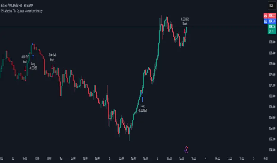
📊 Trading Rules
Long Entry:
When T3 crosses upward, momentum is positive, and the squeeze has just been released.
Short Entry:
When T3 crosses downward, momentum is negative, and the squeeze has just been released.
Exit (Reversal):
When the opposite condition to the entry is triggered, the position is reversed.
💰 Risk Management Parameters
Pair & Timeframe: BTC/USD (30-minute chart)
Capital (simulated): $30,00
Order size: `$100` per trade (realistic, low-risk sizing)
Commission: 0.02%
Slippage: 2 pips
Risk per Trade: 5%
Number of Trades (backtest period): 181
📊 Performance Overview
Symbol: BTC/USD
Timeframe: 30-minute chart
Date Range: January 1, 2024 – July 3, 2025
Win Rate: 47.8%
Profit Factor: 2.01
Net Profit: 173.16 (units not specified)
Max Drawdown: 5.77% or 24.91 (0.79%)
⚙️ Indicator Parameters
Indicator Name: RSI-Adaptive T3 + Squeeze Momentum
RSI Length: 14
T3 Min Length: 5
T3 Max Length: 50
T3 Volume Factor: 0.7
BB Length: 27 (Multiplier: 2.0)
KC Length: 20 (Multiplier: 1.5, TrueRange enabled)
🖼 Visual Support
T3 slope direction, squeeze status, and momentum bars are visually plotted on the chart,
providing high clarity for quick trend analysis and execution.
🔧 Strategy Improvements & Uniqueness
Inspired by the RSI Adaptive T3 by ChartPrime and Squeeze Momentum Indicator by LazyBear ,
this strategy fuses both into a hybrid trend-reversal and momentum breakout detection system .
Compared to traditional trend-following methods, it excels at capturing early trend signals with greater sensitivity .
✅ Summary
The RSI-Adaptive T3 + Squeeze Momentum Strategy combines momentum detection with volatility-responsive risk management.
With a strong balance between visual clarity and practicality, it serves as a powerful tool for traders seeking high repeatability.
⚠️ This strategy is based on historical data and does not guarantee future profits.
Always use appropriate risk management when applying it.
Lazybear
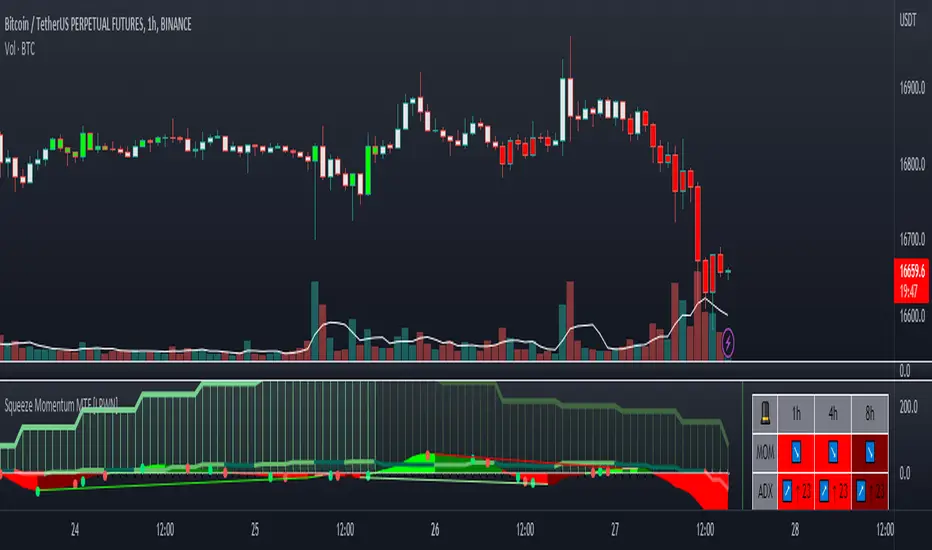
TTM Squeeze Momentum MTF [Cometreon]TTM Squeeze Momentum MTF combines the core logic of both the Squeeze Momentum by LazyBear and the TTM Squeeze by John Carter into a single, unified indicator. It offers a complete system to analyze the phase, direction, and strength of market movements.
Unlike the original versions, this indicator allows you to choose how to calculate the trend, select from 15 different types of moving averages, customize every parameter, and adapt the visual style to your trading preferences.
If you are looking for a powerful, flexible and highly configurable tool, this is the perfect choice for you.
🔷 New Features and Improvements
🟩 Unified System: Trend Detection + Visual Style
You can decide which logic to use for the trend via the "Show TTM Squeeze Trend" input:
✅ Enabled → Trend calculated using TTM Squeeze
❌ Disabled → Trend based on Squeeze Momentum
You can also customize the visual style of the indicator:
✅ Enable "Show Histogram" for a visual mode using Histogram, Area, or Column
❌ Disable it to display the classic LazyBear-style line
Everything updates automatically and dynamically based on your selection.
🟩 Full Customization
Every base parameter of the original indicator is now fully configurable: lengths, sources, moving average types, and more.
You can finally adapt the squeeze logic to your strategy — not the other way around.
🟩 Multi-MA Engine
Choose from 15 different Moving Averages for each part of the calculation:
SMA (Simple Moving Average)
EMA (Exponential Moving Average)
WMA (Weighted Moving Average)
RMA (Smoothed Moving Average)
HMA (Hull Moving Average)
JMA (Jurik Moving Average)
DEMA (Double Exponential Moving Average)
TEMA (Triple Exponential Moving Average)
LSMA (Least Squares Moving Average)
VWMA (Volume-Weighted Moving Average)
SMMA (Smoothed Moving Average)
KAMA (Kaufman’s Adaptive Moving Average)
ALMA (Arnaud Legoux Moving Average)
FRAMA (Fractal Adaptive Moving Average)
VIDYA (Variable Index Dynamic Average)
🟩 Dynamic Signal Line
Apply a moving average to the momentum for real-time cross signals, with full control over its length and type.
🟩 Multi-Timeframe & Multi-Ticker Support
You're no longer limited to the chart's current timeframe or ticker. Apply the squeeze to any symbol or timeframe without repainting.
🔷 Technical Details and Customizable Inputs
This indicator offers a fully modular structure with configurable parameters for every component:
1️⃣ Squeeze Momentum Settings – Choose the source, length, and type of moving average used to calculate the base momentum.
2️⃣ Trend Mode Selector – Toggle "Show TTM Squeeze Trend" to select the trend logic displayed on the chart:
✅ Enabled – Shows the trend based on TTM Squeeze (Bollinger Bands inside/outside Keltner Channel)
❌ Disabled – Displays the trend based on Squeeze Momentum logic
🔁 The moving average type for the Keltner Channel is handled automatically, so you don't need to select it manually, even if the custom input is disabled.
3️⃣ Signal Line – Toggle the Signal Line on the Squeeze Momentum. Select its length and MA type to generate visual cross signals.
4️⃣ Bollinger Bands – Configure the length, multiplier, source, and MA type used in the bands.
5️⃣ Keltner Channel – Adjust the length, multiplier, source, and MA type. You can also enable or disable the True Range option.
6️⃣ Advanced MA Parameters – Customize the parameters for advanced MAs (JMA, ALMA, FRAMA, VIDYA), including Phase, Power, Offset, Sigma, and Shift values.
7️⃣ Ticker & Input Source – Select the ticker and manage inputs for alternative chart types like Renko, Kagi, Line Break, and Point & Figure.
8️⃣ Style Settings – Choose how the squeeze is displayed:
Enable "Show Histogram" for Histogram, Area, or Column style
Disable it to show the classic LazyBear-style line
Use Reverse Color to invert line colors
Toggle Show Label to highlight Signal Line cross signals
Customize trend colors to suit your preferences
9️⃣ Multi-Timeframe Options - Timeframe – Use the squeeze on higher timeframes for stronger confirmation
🔟 Wait for Timeframe Closes -
✅ Enabled – Prevents multiple signals within the same candle
❌ Disabled – Displays the indicator smoothly without delay
🔧 Default Settings Reference
To replicate the default settings of the original indicators as they appear when first applied to the chart, use the following configurations:
🟩 TTM Squeeze (John Carter Style)
Squeeze
Length: 20
MA Type: SMA
Show TTM Squeeze Trend: Enabled
Bollinger Bands
Length: 20
Multiplier: 2.0
MA Type: SMA
Keltner Channel
Length: 20
Multiplier: 1.0
Use True Range: ON
MA Type: EMA
Style
Show Histogram: Enabled
Reverse Color: Enabled
🟩 Squeeze Momentum (LazyBear Style)
Squeeze
Length: 10
MA Type: SMA
Show TTM Squeeze Trend: Disabled
Bollinger Bands
Length: 20
Multiplier: 1.5
MA Type: SMA
Keltner Channel
Length: 10
Multiplier: 1.5
Use True Range: ON
MA Type: SMA
Style
Show Histogram: Disabled
Reverse Color: Disabled
⚠️ These values are intended as a starting point. The Cometreon indicator lets you fully customize every input to fit your trading style.
🔷 How to Use Squeeze Momentum Pro
🔍 Identifying Trends
Squeeze Momentum Pro supports two different methods for identifying the trend visually, each based on a distinct logic:
Squeeze Momentum Trend (LazyBear-style):
Displays 3 states based on the position of the Bollinger Bands relative to the Keltner Channel:
🔵 Blue = No Squeeze (BB outside KC and KC outside BB)
⚪️ White = Squeeze Active (BB fully inside KC)
⚫️ Gray = Neutral state (none of the above)
TTM Squeeze Trend (John Carter-style):
Calculates the difference in width between the Bollinger Bands and the Keltner Channel:
🟩 Green = BB width is greater than KC → potential expansion phase
🟥 Red = BB are tighter than KC → possible compression or pre-breakout
📈 Interpreting Signals
Depending on the active configuration, the indicator can provide various signals, including:
Trend color → Reflects the current compression/expansion state (based on selected mode)
Momentum value (above or below 0) → May indicate directional pressure
Signal Line cross → Can highlight momentum shifts
Color change in the momentum → May suggest a potential trend reversal
🛠 Integration with Other Tools
Squeeze Momentum Pro works well alongside other indicators to strengthen market context:
✅ Volume Profile / OBV – Helps confirm accumulation or distribution during squeezes
✅ RSI – Useful to detect divergence between momentum and price
✅ Moving Averages – Ideal for defining primary trend direction and filtering signals
☄️ If you find this indicator useful, leave a Boost to support its development!
Every piece of feedback helps improve the tool and deliver an even better trading experience.
🔥 Share your ideas or feature requests in the comments!

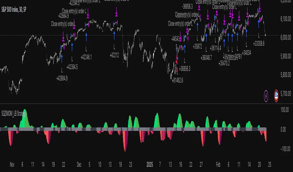
Squeeze Momentum Indicator Strategy [LazyBear + PineIndicators]The Squeeze Momentum Indicator Strategy (SQZMOM_LB Strategy) is an automated trading strategy based on the Squeeze Momentum Indicator developed by LazyBear, which itself is a modification of John Carter's "TTM Squeeze" concept from his book Mastering the Trade (Chapter 11). This strategy is designed to identify low-volatility phases in the market, which often precede explosive price movements, and to enter trades in the direction of the prevailing momentum.
Concept & Indicator Breakdown
The strategy employs a combination of Bollinger Bands (BB) and Keltner Channels (KC) to detect market squeezes:
Squeeze Condition:
When Bollinger Bands are inside the Keltner Channels (Black Crosses), volatility is low, signaling a potential upcoming price breakout.
When Bollinger Bands move outside Keltner Channels (Gray Crosses), the squeeze is released, indicating an expansion in volatility.
Momentum Calculation:
A linear regression-based momentum value is used instead of traditional momentum indicators.
The momentum histogram is color-coded to show strength and direction:
Lime/Green: Increasing bullish momentum
Red/Maroon: Increasing bearish momentum
Signal Colors:
Black: Market is in a squeeze (low volatility).
Gray: Squeeze is released, and volatility is expanding.
Blue: No squeeze condition is present.
Strategy Logic
The script uses historical volatility conditions and momentum trends to generate buy/sell signals and manage positions.
1. Entry Conditions
Long Position (Buy)
The squeeze just released (Gray Cross after Black Cross).
The momentum value is increasing and positive.
The momentum is at a local low compared to the past 100 bars.
The price is above the 100-period EMA.
The closing price is higher than the previous close.
Short Position (Sell)
The squeeze just released (Gray Cross after Black Cross).
The momentum value is decreasing and negative.
The momentum is at a local high compared to the past 100 bars.
The price is below the 100-period EMA.
The closing price is lower than the previous close.
2. Exit Conditions
Long Exit:
The momentum value starts decreasing (momentum lower than previous bar).
Short Exit:
The momentum value starts increasing (momentum higher than previous bar).
Position Sizing
Position size is dynamically adjusted based on 8% of strategy equity, divided by the current closing price, ensuring risk-adjusted trade sizes.
How to Use This Strategy
Apply on Suitable Markets:
Best for stocks, indices, and forex pairs with momentum-driven price action.
Works on multiple timeframes but is most effective on higher timeframes (1H, 4H, Daily).
Confirm Entries with Additional Indicators:
The author recommends ADX or WaveTrend to refine entries and avoid false signals.
Risk Management:
Since the strategy dynamically sizes positions, it's advised to use stop-losses or risk-based exits to avoid excessive drawdowns.
Final Thoughts
The Squeeze Momentum Indicator Strategy provides a systematic approach to trading volatility expansions, leveraging the classic TTM Squeeze principles with a unique linear regression-based momentum calculation. Originally inspired by John Carter’s method, LazyBear's version and this strategy offer a refined, adaptable tool for traders looking to capitalize on market momentum shifts.
Squeeze Momentum DeluxeThe Squeeze Momentum Deluxe is a comprehensive trading toolkit built with features of momentum, volatility, and price action. This script offers a suite for both mean reversion and trend-following analysis. Developed based on the original TTM Squeeze implementation by @LazyBear, this indicator introduces several innovative components to enhance your trading insights.
🔲 Components and Features
Momentum Oscillator - as rooted in the TTM Squeeze, quantifies the relationship between price and its extremes over a defined period. By normalizing the calculation, the values become comparable throughout time and across securities, allowing for a nuanced assessment of Bullish and Bearish momentum. Furthermore, by presenting it as a ribbon with a signal line we gain additional information about the direction of price swings.
Squeeze Bars - The original squeeze concept is based on the relationship between the Bollinger Bands and Keltner Channel , once the BB resides inside the KC a squeeze occurs. By understanding their fundamentals a new form of calculation can be inferred.
method bb(float src, simple int len, simple float mult) => method kc(float src, simple int len, simple float mult) =>
float basis = ta.sma (src, len) float basis = ta.sma (src, len)
float dev = ta.stdev(src, len) float rng = ta.atr ( len)
float upper = basis + dev * mult float upper = basis + rng * mult
float lower = basis - dev * mult float lower = basis - rng * mult
Both BB and KC are constructed upon a moving average with the addition of Standard Deviation and Average True Range respectively. Therefore, the calculation can be transformed to when the Stdev is lower than the ATR a squeeze occurs.
method sqz(float src, simple int len) =>
float dev = ta.stdev(src, len)
float atr = ta.atr ( len)
dev < atr ? true : false
This indicator uses three different thresholds for the ATR to gain three levels of price "Squeeze" for further analysis.
Directional Flux- This component measures the overall direction of price volatility, offering insights into trend sentiment. Presented as waves in the background, it includes an OverFlux feature to signal extreme market bias in a particular direction which can signal either exhaustion or vital continuation. Additionally, the user can choose if to base the calculation on Heikin-Ashi Candles to bias the tool toward trend assessment.
Confluence Gauges - Placed at the top and bottom of the indicator, these gauges measure confluence in the relationship between the Momentum Oscillator and Directional Flux. They provide traders with an easily interpretable visual aid for detecting market sentiment. Reversal doritos displayed alongside them contribute to mean reversion analysis.
Divergences (Real-Time) - Equipped with a custom algorithm, the indicator detects real-time divergences between price and the oscillator. This dynamic feature enhances your ability to spot potential trend reversals as they occur.
🔲 Settings
Directional Flux Length - Adjusts the period of which the background volatility waves operate on.
Trend Bias - Bases the calculation of the Flux to HA candles to bias its behavior toward the trend of price action.
Squeeze Momentum Length - Calibrates the length of the main oscillator ribbon as well as the period for the squeeze algorithm.
Signal - Controls the width of the ribbon. Lower values result in faster responsiveness at the cost of premature positives.
Divergence Sensitivity - Adjusts a threshold to limit the amount of divergences detected based on strength. Higher values result in less detections, stronger structure.
🔲 Alerts
Sell Signal
Buy Signal
Bullish Momentum
Bearish Momentum
Bullish Flux
Bearish Flux
Bullish Swing
Bearish Swing
Strong Bull Gauge
Strong Bear Gauge
Weak Bull Gauge
Weak Bear Gauge
High Squeeze
Normal Squeeze
Low Squeeze
Bullish Divergence
Bearish Divergence
As well as the option to trigger 'any alert' call.
The Squeeze Momentum Deluxe is a comprehensive tool that goes beyond traditional momentum indicators, offering a rich set of features to elevate your trading strategy. I recommend using toolkit alongside other indicators to have a wide variety of confluence to therefore gain higher probabilistic and better informed decisions.

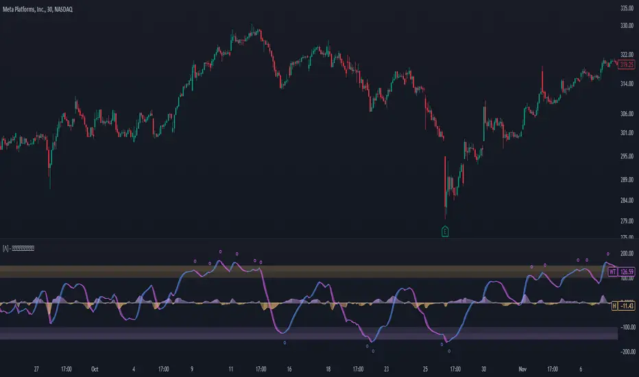
Enhanced WaveTrend OscillatorThe Enhanced WaveTrend Oscillator is a modified version of the original WaveTrend. The WaveTrend indicator is a popular technical analysis tool used to identify overbought and oversold conditions in the market and generate trading signals. The enhanced version addresses certain limitations of the original indicator and introduces additional features for improved analysis and comparison across assets.
WaveTrend:
The original WaveTrend indicator calculates two lines based on exponential moving averages and their relationship to the asset's price. The first line measures the distance between the asset's price and its EMA, while the second line smooths the first line over a specific period. The result is divided by 0.015 multiplied by the smoothed difference ('d' for reference). The indicator aims to identify overbought and oversold conditions by analyzing the relationship between the two lines.
In the original formula, the rudimentary estimation factor 0.015 times 'd' fails to accomodate for approximately a quarter of the data, preventing the indicator from reaching the traditional stationary levels of +-100. This limitation renders the indicator quantitatively biased, as it relies on the user's subjective adjustment of the levels. The enhanced version replaces this factor with the standard deviation of the asset's price, resulting in improved estimation accuracy and provides a more dynamic and robust outcome, we thereafter multiply the result by 100 to achieve a more traditional oscillation.
Enhancements and Features:
The enhanced version of the WaveTrend indicator addresses several limitations of the original indicator and introduces additional features-
Dynamic Estimation: The original indicator uses an arbitrary estimation factor, while the enhanced version replaces it with the standard deviation of the asset's price. This modification provides a more dynamic and accurate estimation, adapting to the specific price characteristics of each asset.
Stationary Support and Resistance Levels: The enhanced version provides stationary key support and resistance levels that range from -150 to 150. These levels are determined based on the analysis of the indicator's data and encompass more than 95% of the indicator's values. These levels offer important reference points for traders to identify potential price reversals or significant price movements.
Comparison Across Assets: The enhanced version allows for better comparison and analysis across different assets. By incorporating the standard deviation of the asset's price, the indicator provides a more consistent and comparable interpretation of the market conditions across multiple assets.
Upon closer inspection of the modification in the enhanced version, we can observe that the resulting indicator is a smoothed variation of the Z-Score!
f_ewave(src, chlen, avglen) =>
basis = ta.ema(src, chlen)
dev = ta.stdev(src, chlen)
wave = (src - basis) / dev * 100
ta.ema(wave, avglen)
Z-Score Analysis:
The Z-Score is a statistical measurement that quantifies how far a particular data point deviates from the mean in terms of standard deviations. In the enhanced version, the calculation involves determining the basis (mean) and deviation (standard deviation) of the asset's price to calculate its Z-Score, thereafter applying a smoothing technique to generate the final WaveTrend value.
Utility:
The 𝗘𝗻𝗵𝗮𝗻𝗰𝗲𝗱 𝗪𝗧 indicator offers traders and investors valuable insights into overbought and oversold conditions in the market. By analyzing the indicator's values and referencing the stationary support and resistance levels, traders can identify potential trend reversals, evaluate market strength, and make better informed analysis.
It is important to note that this indicator should be used in conjunction with other technical analysis tools and indicators to confirm trading signals and validate market dynamics.
Credit:
The 𝗘𝗻𝗵𝗮𝗻𝗰𝗲𝗱 𝗪𝗧 indicator is a modification of the original WaveTrend Oscillator developed by @LazyBear on TradingView.
Example Charts:
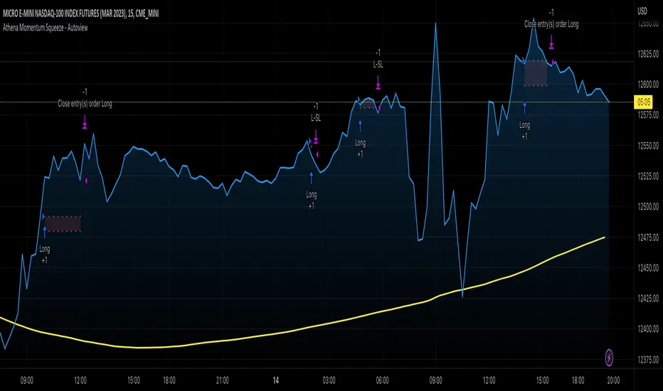
Athena Momentum Squeeze - Short, Lean, and Mean This is a very profitable strategy focusing on 15 minute intervals on the Micro Nasdaq Futures contracts. CME_MINI:MNQH2023
As this contract only keeps positions for on average about an hour risk is managed. At a profit factor of 3.382 with a max drawdown of $123 from January 1st to February 15. Looking back to Dec 2019 still maintains a profit factor of 1.3.
See backtesting: www.screencast.com
2019 backtesting: www.screencast.com
Based on the classic Lazy Bear Oscillator Squeeze with a number of modifications from ADX, MAs and adding fibonacci levels.
We like keeping strategies simple yet powerful, no completely where you can't understand your own trades.
Our team is always modifying and improving the strategy. Always open to collaborating on improving as there is no perfect strategy. www.screencast.com
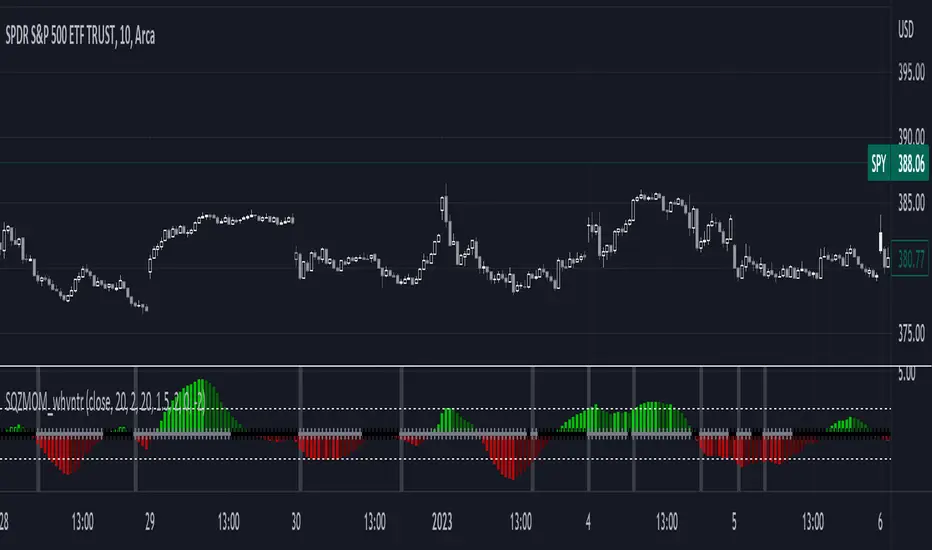
1st Gray Cross Signals ━ Histogram SQZMOM [whvntr][LazyBear]This is the Histogram Version of one of my other indicators named: SQZ Momentum + 1st Gray Cross Signals (with arrows) Which is a modification of "Squeeze Momentum Indicator" by user: "LazyBear". In that indicator of his he described, and suggested, the use of his gray cross signals to find points of interest for trading based on the direction of momentum when the first gray cross appears... I have programmed these points, and highlighted them, for ease of use. The 1st gray cross strategy, he said , is from John F. Carter's book, Chapter 11, "Mastering the Trade".
Here we have the Histogram version, with background highlights only, and nothing on the chart, in true SQZ Momentum style.
Disclaimer: using this indicator, or any indicator anywhere, involves risk when trading and isn't a guarantee of 100% accurate results.
[LazyBear] SQZ Momentum + 1st Gray Cross Signals ━ whvntrI have modified LazyBears Squeeze Momentum Indicator with enhancements, plus added signals
LazyBear mentioned that in John F. Carter's book, Chapter 11, "Mastering the Trade", that "Mr. Carter suggests waiting till the first gray after a black cross, and taking a position in the direction of the momentum (for ex., if momentum value is above zero, go long). Exit the position when the momentum changes (increase or decrease --- signified by a color change)." I have done just that. Now at each "first gray after a black cross", there are now Bearish and Bullish signals.. The signals only appear in the direction of the momentum.
Disclaimer: This indicator does not constitute investment advice. Trade at your own
risk with this method of identifying changes in stock market momentum.

Squeeze Momentum MTF [LPWN]//ENGLISH
Squeeze momentum of lazy bear, multiple time frames, It gives you information if the cycles with high temporality momentums are in harmony, by default two more momentums are shown, I prefer to use only one extra, in the options you can change the time frame of the momentums, in addition to the momentums you can add the RSI and ADX, if the momentum look small, you can change the value of general scale to make them bigger, the table gives us information on how the momentums and the adx are, in the options you can set the candles to color according to the harmony of the momentums
// SPANISH
Squeeze momentum de lazy bear, multiple time frames, te da informacion si los ciclos con momentums de temporalidad alta estan en armonia,por defecto se muestran dos momentums mas, yo prefiero usar solo uno extra, en las opcoines puedes cambiar la temporalidad de los momentums, ademas de los momentums puedes agregar el RSI y el ADX, si el momentum se ve pequeño, puedes cambiar el valor de general scale para hacerlos mas grandes, la tabla nos da infomracion de como estan los momentums y el adx, en las opciones puedes poner que las velas se pongan del color de acuerdo a la armonia de los momentums
WaveTrend 3D█ OVERVIEW
WaveTrend 3D (WT3D) is a novel implementation of the famous WaveTrend (WT) indicator and has been completely redesigned from the ground up to address some of the inherent shortcomings associated with the traditional WT algorithm.
█ BACKGROUND
The WaveTrend (WT) indicator has become a widely popular tool for traders in recent years. WT was first ported to PineScript in 2014 by the user @LazyBear, and since then, it has ascended to become one of the Top 5 most popular scripts on TradingView.
The WT algorithm appears to have origins in a lesser-known proprietary algorithm called Trading Channel Index (TCI), created by AIQ Systems in 1986 as an integral part of their commercial software suite, TradingExpert Pro. The software’s reference manual states that “TCI identifies changes in price direction” and is “an adaptation of Donald R. Lambert’s Commodity Channel Index (CCI)”, which was introduced to the world six years earlier in 1980. Interestingly, a vestige of this early beginning can still be seen in the source code of LazyBear’s script, where the final EMA calculation is stored in an intermediate variable called “tci” in the code.
█ IMPLEMENTATION DETAILS
WaveTrend 3D is an alternative implementation of WaveTrend that directly addresses some of the known shortcomings of the indicator, including its unbounded extremes, susceptibility to whipsaw, and lack of insight into other timeframes.
In the canonical WT approach, an exponential moving average (EMA) for a given lookback window is used to assess the variability between price and two other EMAs relative to a second lookback window. Since the difference between the average price and its associated EMA is essentially unbounded, an arbitrary scaling factor of 0.015 is typically applied as a crude form of rescaling but still fails to capture 20-30% of values between the range of -100 to 100. Additionally, the trigger signal for the final EMA (i.e., TCI) crossover-based oscillator is a four-bar simple moving average (SMA), which further contributes to the net lag accumulated by the consecutive EMA calculations in the previous steps.
The core idea behind WT3D is to replace the EMA-based crossover system with modern Digital Signal Processing techniques. By assuming that price action adheres approximately to a Gaussian distribution, it is possible to sidestep the scaling nightmare associated with unbounded price differentials of the original WaveTrend method by focusing instead on the alteration of the underlying Probability Distribution Function (PDF) of the input series. Furthermore, using a signal processing filter such as a Butterworth Filter, we can eliminate the need for consecutive exponential moving averages along with the associated lag they bring.
Ideally, it is convenient to have the resulting probability distribution oscillate between the values of -1 and 1, with the zero line serving as a median. With this objective in mind, it is possible to borrow a common technique from the field of Machine Learning that uses a sigmoid-like activation function to transform our data set of interest. One such function is the hyperbolic tangent function (tanh), which is often used as an activation function in the hidden layers of neural networks due to its unique property of ensuring the values stay between -1 and 1. By taking the first-order derivative of our input series and normalizing it using the quadratic mean, the tanh function performs a high-quality redistribution of the input signal into the desired range of -1 to 1. Finally, using a dual-pole filter such as the Butterworth Filter popularized by John Ehlers, excessive market noise can be filtered out, leaving behind a crisp moving average with minimal lag.
Furthermore, WT3D expands upon the original functionality of WT by providing:
First-class support for multi-timeframe (MTF) analysis
Kernel-based regression for trend reversal confirmation
Various options for signal smoothing and transformation
A unique mode for visualizing an input series as a symmetrical, three-dimensional waveform useful for pattern identification and cycle-related analysis
█ SETTINGS
This is a summary of the settings used in the script listed in roughly the order in which they appear. By default, all default colors are from Google's TensorFlow framework and are considered to be colorblind safe.
Source: The input series. Usually, it is the close or average price, but it can be any series.
Use Mirror: Whether to display a mirror image of the source series; for visualizing the series as a 3D waveform similar to a soundwave.
Use EMA: Whether to use an exponential moving average of the input series.
EMA Length: The length of the exponential moving average.
Use COG: Whether to use the center of gravity of the input series.
COG Length: The length of the center of gravity.
Speed to Emphasize: The target speed to emphasize.
Width: The width of the emphasized line.
Display Kernel Moving Average: Whether to display the kernel moving average of the signal. Like PCA, an unsupervised Machine Learning technique whereby neighboring vectors are projected onto the Principal Component.
Display Kernel Signal: Whether to display the kernel estimator for the emphasized line. Like the Kernel MA, it can show underlying shifts in bias within a more significant trend by the colors reflected on the ribbon itself.
Show Oscillator Lines: Whether to show the oscillator lines.
Offset: The offset of the emphasized oscillator plots.
Fast Length: The length scale factor for the fast oscillator.
Fast Smoothing: The smoothing scale factor for the fast oscillator.
Normal Length: The length scale factor for the normal oscillator.
Normal Smoothing: The smoothing scale factor for the normal frequency.
Slow Length: The length scale factor for the slow oscillator.
Slow Smoothing: The smoothing scale factor for the slow frequency.
Divergence Threshold: The number of bars for the divergence to be considered significant.
Trigger Wave Percent Size: How big the current wave should be relative to the previous wave.
Background Area Transparency Factor: Transparency factor for the background area.
Foreground Area Transparency Factor: Transparency factor for the foreground area.
Background Line Transparency Factor: Transparency factor for the background line.
Foreground Line Transparency Factor: Transparency factor for the foreground line.
Custom Transparency: Transparency of the custom colors.
Total Gradient Steps: The maximum amount of steps supported for a gradient calculation is 256.
Fast Bullish Color: The color of the fast bullish line.
Normal Bullish Color: The color of the normal bullish line.
Slow Bullish Color: The color of the slow bullish line.
Fast Bearish Color: The color of the fast bearish line.
Normal Bearish Color: The color of the normal bearish line.
Slow Bearish Color: The color of the slow bearish line.
Bullish Divergence Signals: The color of the bullish divergence signals.
Bearish Divergence Signals: The color of the bearish divergence signals.
█ ACKNOWLEDGEMENTS
@LazyBear - For authoring the original WaveTrend port on TradingView
@PineCoders - For the beautiful color gradient framework used in this indicator
@veryfid - For the inspiration of using mirrored signals for cycle analysis and using multiple lookback windows as proxies for other timeframes

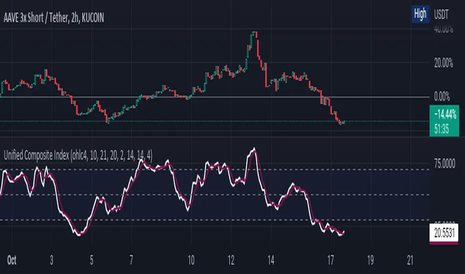
Unified Composite Index [UCI] [KuraiBlu] [LazyBear]The purpose of this indicator is to combine the four basic types of indicators (Trend, Volatility, Momentum and Volume) to create a singular, composite index in order to provide a more holistic means of observing potential changes within the market, known as the Unified Composite Index . The indicators used in this index are as follows:
Trend - Trend Composite Index
Volatility - Bollinger Bands %b
Momentum - Relative Strength Index
Volume - Money Flow Index
The average price source can’t be altered as I’ve made it an average between ((open + close) / 2) and ((high + low) / 2).
The best way to use this is by observing several of the indicators at once in conjunction with the average, rather than simply using the average produced to determine the right moment to enter, or exit a trade by itself. I've found when one indicator goes way out of bounds relative to the other three (and subsequently, the average array), then it presents a good buying, or selling opportunity.
Some adjustments were made to several of the indicators in order to standardize them on a scale of 1-100 so that they could better accommodate the average array that was finally produced. Thanks to LazyBear for letting me strip down the WaveTrend Oscillator.
WaveTrend 4h/24mWaveTrend 4h/24m is a trading tool based on two WaveTrend timeframes.
For this script the WaveTrend calculations made by LazyBear were used. WaveTrend is a widely used indicator for finding direction of an asset.
The strategy is developed by Youtuber Jayson Casper. The main strategy on the 4 hour and 24 minute timeframes, this will be the default timeframes. Timeframes can be adjusted in the indicator interface.
With Jaysons' we wait for both timeframes to have last printed a green dot for longs, and both timeframes to have last printed a red dot for shorts. When this occurs a green diamond will be printed for longs, a red diamond for shorts.
Make sure to always use the chart from the smallest timeframe you're using, so by defaults use the 24 minute chart.
Features of the indicator:
- WaveTrend Timeframe 1 (Blue/Lightblue wave).
- WaveTrend Timeframe 2 (Blue/Purple line with filled background between the lines).
- VWAP (Yellow wave which is turned off by default)
- Green/Red Diamonds
What to look for?
This script is all about the Green and Red Diamonds.
A Green diamond will be printed when on both the 4 hour and 24 minute timeframe the last printed dot was a green dot.
A Red diamond will be printed when on both the 4 hour and 24 minute timeframe the last printed dot was a red dot.
What are the Green and Red Diamonds based on?
When both VWAP timeframes are ABOVE 0, a green diamond will be printed. This is equivalent to the last dot on both WaveTrend timeframes being a green dot.
When both VWAP timeframes are BELOW 0, a red diamond will be printed. This is equivalent to the last dot on both WaveTrend timeframes being a red dot.
Happy Trading!

Visual Squeeze MomentumSqueeze Momentum from LazyBear now visible at the chart so you can check when the Squeeze its about to release. All credits for him.

Crypto momentum strategyThis strategy is based on LazyBear's Squeeze Momentum indicator. It analyzes when the trend in the momentum is shifting, locating the peaks and the valleys, and takes those as sell and buy signals respectively. This is a long strategy, so it also takes into consideration the 50 period Exponential Moving Average to identify upward trends. If the closing price of the candle is above the 50EMA, and the slope of the 50EMA is trending upwards, then the buy signal is executed. If these conditions are not met, the buy signal is ignored.
This strategy works well with crypto trading on the day/week charts.
It has a profit ratio of 4:1 on average, and roughly half of the trades are profitable.

Squeeze Momentum Indicator MTF with alerts [lazy bear]MTF version of the popular squeeze momentum indicator, created and shared by Lazy Bear

WaveTrend [LazyBear] vX by DGTDGT interpreted version of LazyBear's WaveTrend, visualizing on Price Chart
Original Author : LazyBear
Crosses above or below threshold are emphasized with bigger labels
- crosses above threshold : probable short indications with a bigger label and relativly small label for probable long indications
- crosses below threshold : probable long indications with a bigger label and relativly small label for probable short indications
All rest crosses within threshold boundaries with relatively small labels for both long and short probable indications
Squeeze Momentum Indicator [LazyBear] vHMAThis is a remake of the famous LazyBear Indicator, the Squeeze Momentum Indicator.
All i did was take out the SMA's and replace them with HMA's. HMA is a more responsive moving average.
Hull Moving Average.
This is a derivative of John Carter's "TTM Squeeze" volatility indicator, as discussed in his book "Mastering the Trade" (chapter 11).
Black crosses on the midline show that the market just entered a squeeze ( Bollinger Bands are with in Keltner Channel). This signifies low volatility , market preparing itself for an explosive move (up or down). Gray crosses signify "Squeeze release".
Mr.Carter suggests waiting till the first gray after a black cross, and taking a position in the direction of the momentum (for ex., if momentum value is above zero, go long). Exit the position when the momentum changes (increase or decrease --- signified by a color change). My (limited) experience with this shows, an additional indicator like ADX / WaveTrend, is needed to not miss good entry points. Also, Mr.Carter uses simple momentum indicator , while I have used a different method (linreg based) to plot the histogram.
More info:
- Book: Mastering The Trade by John F Carter
Here is the original version:

OBV with DivergenceAll I did was combine the logic from LazyBear for his OBV Oscillator to regular RSI divergence logic (where I replaced the RSI input to use LazyBear's OBV).
I didn't use any original code! Neither OBV (written by LazyBear) nor DIvergence (author unknown) was written by me. I merely modified the sytax a little to combine them.
Very useful for spotting divergences with OBV oscillator.

Code Upd: Weis Wave Volume [LazyBear] v4One of the review indicator from me.
I reviewed code for more comfortable use - the basic code was not modified.
Enjoy it!

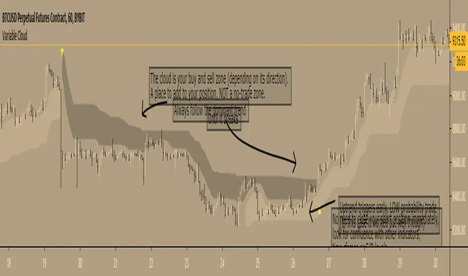
Variable Cloud - evoA Super Trend based on the high and low of a Moving Average, to get an easy view what the current trend is and where to buy and sell.
TIPS
- The 'Closing Source' option is the candle value that triggers the clouds. 'High/Low System' means that a downtrend is over when the candle LOW closes greater than the downtrend (dark cloud), an uptrend is over when the candle HIGH closes less than the uptrend (light cloud). The other options speak for themselves.
- Ideally place your stop loss outside the cloud, as you want to stay in the trend until it breaks to the opposite direction (but that's up to you of course).
- Reversal trades are low probability, you can see them as reversals or ranging before the market continues, I like to lower my risk on those set ups till it breaks the dominant trend.
Here are the scripts I used:
Everget's SuperTrend
LazyBear's VMA
Thanks LazyBear and Everget, I learn a lot from your scripts :)
Waddah Attar Explosion MTFAll I did here is add multi timeframe function to the Waddah Attar indicator, as I couldn't find it in the TradingView library.
A description of the original post by Lazy Bear

Divergence of DecisionPoint Breadth Swenlin Trading [LazyBear]// This source code is subject to the terms of the Mozilla Public License 2.0 at mozilla.org
// © 03.freeman
//This is indicator from LazyBear is very accurate for stocks and indexes.
//I added some code snippets for spot and draw divergences automatically
//
// @author LazyBear
//
//
Best use with daily time frame.
Enter when a divergence is found (Bull or Bear label) and wait at least a couple of candles before exit.
Next improvement: alerts ready made for webhooks and screener for multiple tickers.
Please use comment section for any feedback.

Study for Squeeze Momentum Indicator [LazyBear]This study is based on LazyBear Squeeze Momentum Indicator and my strategy developed using it.
I added some custom feature and filters.
Main improvements are:
1- study is updated to version 4 of pine script;
2- I added alerts for entry rules and exit rules.
3- Alert syntax can be customized for webhooks: I added one example only for long entry.
You can customize a lot of features to get a profitable strategy.
Here is a link to original study.
Please use comment section for any feedback.
