Global Liquidity Indicator in USDThis indicator aggregates the total central bank balance sheets and M2 money supply for the USA, Canada, China, European Union, Japan, and the UK, converting all values to USD and normalizing them to trillions for easy visualization. It plots three lines: Total Balance Sheet, Total M2, and Combined Total, providing a comprehensive view of global liquidity trends.
Key Features:
Dynamic Coloring: Customize line colors based on direction—green for upward trends, red for downward (or any colors you choose), with independent on/off toggles for each line.
Real-Time Currency Conversion: Uses live forex rates (e.g., USD/CNY, USD/EUR) for accurate USD conversions.
Forecasting

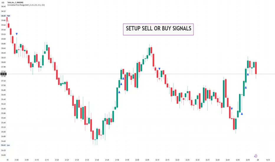
Cumulative Price Change AlertCumulative Price Change Alert
Version: 1.0
Author: QCodeTrader 🚀
Overview 🔍
The Cumulative Price Change Alert indicator analyzes the percentage change between the current and previous open prices and sums these changes over a user-defined number of bars. It then generates visual buy and sell signals using arrows and labels on the chart, helping traders spot cumulative price momentum and potential trading opportunities.
Key Features ⚙️
Customizable Timeframe 🕒:
Use a custom timeframe or default to the chart's timeframe for price data.
User-Defined Summation 🔢:
Specify the number of bars to sum, allowing you to analyze cumulative price changes.
Custom Buy & Sell Conditions 🔔:
Set individual percentage change thresholds and cumulative sum thresholds to tailor signals for
your strategy.
Visual Alerts 🚀:
Displays green upward arrows for buy signals and red downward arrows for sell signals directly
on the chart.
Informative Labels 📝:
Provides labels with formatted percentage change and cumulative sum details for the analyzed
bars.
Versatile Application 📊:
Suitable for stocks, forex, crypto, commodities, and more.
How It Works ⚡
Price Change Calculation ➗:
The indicator calculates the percentage change between the current bar's open price and the
previous bar's open price.
Cumulative Sum ➕:
It then sums these percentage changes over the last N bars (as specified by the user).
Signal Generation 🚦:
Buy Signal 🟢: When both the individual percentage change and the cumulative sum exceed
their respective buy thresholds, a green arrow and label are displayed.
Sell Signal 🔴: Conversely, if the individual change and cumulative sum fall below the sell
thresholds, a red arrow and label are shown.
How to Use 💡
Add the Indicator ➕:
Apply the indicator to your chart.
Customize Settings ⚙️:
Set a custom timeframe if desired.
Define the number of bars to sum.
Adjust the buy/sell percentage change and cumulative sum thresholds to match your trading
strategy.
Interpret Visual Cues 👀:
Monitor the chart for green or red arrows and corresponding labels that signal potential buy or
sell opportunities based on cumulative price movements.
Settings Explained 🛠️
Custom Timeframe:
Select an alternative timeframe for analysis, or leave empty to use the current chart's timeframe.
Number of Last Bars to Sum:
Determines how many bars are used to compute the cumulative percentage change.
Buy Condition - Min % Change:
The minimum individual percentage change required to consider a buy signal.
Buy Condition - Min Sum of Bars:
The minimum cumulative percentage change over the defined bars needed for a buy signal.
Sell Condition - Max % Change:
The maximum individual percentage change threshold for a sell signal.
Sell Condition - Max Sum of Bars:
The maximum cumulative percentage change over the defined bars for triggering a sell signal.
Best Use Cases 🎯
Momentum Identification 📈:
Quickly spot strong cumulative price movements and momentum shifts.
Entry/Exit Signals 🚪:
Use the visual signals to determine potential entry and exit points in your trading.
Versatile Strategy Application 🔄:
Effective for scalping, swing trading, and longer-term analysis across various markets.
UPD: uncheck labels for better performance
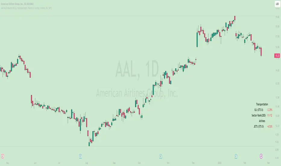
Sector/Industry Relative StrengthOverview
The Sector/Industry Relative Strength (RS) Indicator is a powerful tool designed to help traders and investors analyze the performance of sectors and industries relative to the broader market (SPY). It provides real-time insights into sector and industry strength, helping you identify leading and lagging areas of the market.
Key Features
Sector and Industry Analysis:
Automatically detects the sector and industry of the current symbol.
Displays the corresponding sector and industry ETF.
Relative Strength (STS) Calculation:
Calculates the Sector/Industry Trend Strength (STS) by comparing the sector or industry ETF to SPY over the past 20 days.
STS is expressed as a percentile (0-100), indicating how strong the sector/industry ETF has been relative to SPY over the past 20 days.
Example: An STS of 70 means that during the past 20 days, the ETF’s relative strength against SPY was stronger than 70% of those days.
Sector Rank:
Ranks the current sector ETF against a predefined list of major sector ETFs.
Highlights whether the sector is outperforming or underperforming SPY (green if outperforming, red if underperforming).
Customizable Display:
Choose which elements to display (e.g., sector, industry, ETFs, STS, sector rank).
Customize table position, size, text alignment, and colors.
Real-Time Performance:
Tracks daily price changes for sector and industry ETFs.
Displays percentage change from open to close.
How to Use
Add the Indicator:
Apply the indicator to any stock or ETF chart.
The script will automatically detect the sector and industry of the selected symbol.
Interpret the Data:
Sector/Industry: Displays the current sector and industry.
ETF: Shows the corresponding sector and industry ETF.
STS (Sector/Industry Trend Strength): A percentile score (0-100) indicating the relative strength of the sector/industry ETF compared to SPY over the past 20 days.
Sector Rank: Ranks the sector ETF against other major sectors (e.g., "3/12" means the sector is ranked 3rd out of 12).
Customize the Display:
Use the input settings to:
Show/hide specific elements (e.g., sector, industry, ETFs, STS, sector rank).
Adjust the table position, size, and text alignment.
Change colors for positive/negative changes.
Make Informed Decisions:
Use the STS score and sector rank to identify potential trading opportunities.
Focus on sectors and industries with high STS scores and strong rankings (green).
Input Parameters
Table Settings:
Table Position: Choose where to display the table (Top Left, Top Right, Bottom Left, Bottom Right).
Table Size: Adjust the size of the table (Tiny, Small, Normal, Large).
Text Color: Customize the text color.
Background Color: Set the table background color.
Display Options:
Show ETFs: Toggle the display of sector and industry ETFs.
Show STS: Toggle the display of the Sector/Industry Trend Strength (STS) score.
Show Sector/Industry: Toggle the display of sector and industry information.
Show Sector Rank: Toggle the display of the sector rank.
Parameters:
Sector Rank Time Length: Set the number of days used for calculating the sector rank (default: 20).
Example Use Cases
Sector Rotation:
Identify sectors with high STS scores and strong rankings (green) to allocate capital.
Avoid sectors with low STS scores and weak rankings (red).
Industry Analysis:
Compare the STS scores of different industries within the same sector.
Use the STS score to gauge relative strength and identify potential opportunities.
Market Timing:
Use the STS score and sector rank to time entries and exits in sector-specific ETFs.
Combine with other technical indicators for confirmation.
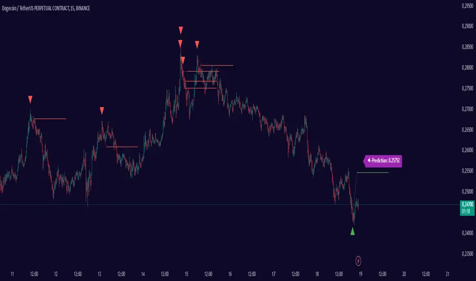
6-Hour Forecast (15m Steps) with Arrowed Lines & 95% CI -BesharaExplanation
Timeframe Conversion:
The helper function converts the chart’s timeframe (e.g., "15", "1H", etc.) into minutes so that the script can determine how many bars correspond to a 15‑minute interval.
Regression & Forecasting:
The script calculates a linear regression over the specified number of bars, approximates the slope, and computes the standard deviation of the residuals for error estimation. Then, for each forecast step (every 15 minutes for 6 hours), it extrapolates the forecast, calculates the 95% confidence interval, and draws red line segments connecting forecast points.
Visualization:
Arrows: At each forecast point, an arrow (▲ for upward, ▼ for downward, or → for unchanged) is drawn to indicate direction.
Confidence Intervals: Dotted orange lines display the 95% confidence interval at each forecast point.
Final Label: A label at the final forecast point shows the predicted price and its confidence interval.
Historical Regression: The blue line represents the historical regression line.
This script is provided for educational purposes only and does not guarantee predictive accuracy. Always use multiple tools and proper risk management in trading.

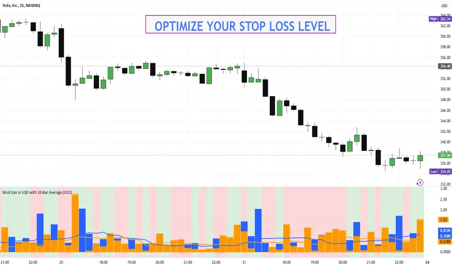
Wick Size in USD with 10-Bar AverageWick Size in USD with 10-Bar Average
Version: 1.0
Author: QCodeTrader
🔍 Overview
This indicator converts the price wicks of your candlestick chart into USD values based on ticks, providing both raw and smoothed data via a 10-bar simple moving average. It helps traders visualize the monetary impact of price extremes, making it easier to assess volatility, potential risk, and plan appropriate stop loss levels.
⚙️ Key Features
Tick-Based Calculation:
Converts wick sizes into ticks (using a fixed tick size of 0.01, typical for stocks) and then into USD using a customizable tick value.
10-Bar Moving Average:
Smooths out the wick values over the last 10 bars, giving you a clearer view of average wick behavior.
Bullish/Bearish Visual Cues:
The chart background automatically highlights bullish candles in green and bearish candles in red for quick visual assessment.
Stop Loss Optimization:
The indicator highlights long wick sizes, which can help you set more accurate stop loss levels. Even when the price moves in your favor, long wicks may indicate potential reversals—allowing you to account for this risk when planning your stop losses.
User-Friendly Customization:
Easily adjust the USD value per tick through the settings to tailor the indicator to your specific instrument.
📊 How It Works
Wick Calculation:
The indicator calculates the upper and lower wicks by measuring the distance between the candle’s high/low and its body (open/close).
Conversion to Ticks & USD:
These wick sizes are first converted from price points to ticks (dividing by a fixed tick size of 0.01) and then multiplied by the user-defined tick value to convert the measurement into USD.
Smoothing Data:
A 10-bar simple moving average is computed for both the upper and lower wick values, providing smoothed data that helps identify trends and deviations.
Visual Representation:
Columns display the raw wick sizes in USD.
Lines indicate the 10-bar moving averages.
Background Color shifts between green (bullish) and red (bearish) based on candle type.
⚡ How to Use
Add the Indicator:
Apply it to your chart to begin visualizing wick sizes in monetary terms.
Customize Settings:
Adjust the Tick Value in USD in the settings to match your instrument’s tick value.
(Note: The tick size is fixed at 0.01, which is standard for many stocks.)
Optimize Your Stop Loss:
Analyze the raw and averaged wick values to understand volatility. Long wicks—even when the price moves in your favor—may indicate potential reversals. This insight can help you set more accurate stop loss levels to protect your gains.
Analyze:
Use the indicator’s data to gauge market volatility and assess the significance of price movements, aiding in more informed trading decisions.
This indicator is perfect for traders looking to understand the impact of extreme price movements in monetary terms, optimize stop loss levels, and effectively manage risk across stocks and other instruments with similar tick structures.
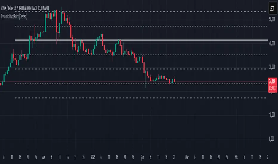
Dynamic Pivot PointsDynamic Pivot Point Indicator
The Dynamic Pivot Point is an indicator used on the TradingView platform that dynamically calculates pivot points and displays them on the chart. This indicator provides automatically adjustable support and resistance levels for different timeframes. By visualizing dynamic levels that match current market conditions, traders can plan their strategies more effectively.
Features
Adapts to Timeframes
The indicator automatically selects the appropriate pivot calculation method based on the user's current timeframe. For example:
For short timeframes such as 1, 3, or 5 minutes, it uses daily (1D) data.
For medium timeframes like 15, 30, or 60 minutes, it uses weekly (1W) data.
For longer timeframes such as 120, 180, or 240 minutes, it uses monthly (1M) data.
For very long timeframes like 360, 480 minutes, daily (D), or weekly (1W), it uses 12-month (12M) data.
Dynamic Pivot Levels
The indicator automatically calculates pivot levels based on the specified high and low values.
Flexible Line Style Options
Users can choose different line styles (Dashed, Dotted, Solid) to improve visual clarity on the chart.
Clean and Clear Visualization
The indicator automatically removes previous lines and displays the latest levels clearly on the chart, preventing clutter and allowing traders to focus more efficiently.
How It Works
Identifying High and Low Levels
The indicator retrieves previous and current high and low levels based on the selected timeframe.
New high and low levels are updated by comparing them with previous levels.
Calculating Pivot Levels
Pivot points are calculated using Fibonacci ratios between high and low levels.
These levels represent dynamic support and resistance zones.
Drawing Lines
The calculated levels are displayed as lines on the chart, each represented with different colors and styles.
Use Cases
Support and Resistance Levels
The indicator dynamically calculates and displays support and resistance levels, serving as reference points for buy and sell decisions.
Trend Analysis
Fibonacci levels help identify trend strength and potential reversal points.
Risk Management
Pivot points assist in setting stop-loss and take-profit levels.
Multi-Timeframe Analysis
Since the indicator adapts to different timeframes, it can be used for both short-term and long-term analysis.
Advantages
✅ Automatic Calculation: No manual calculations are required, as it updates dynamically.
✅ Flexible Timeframe Support: Adapts to different timeframes.
✅ Visual Clarity: Line styles and colors make it easy to distinguish levels on the chart.
✅ Fibonacci Integration: Adds depth to technical analysis.
Conclusion
The Dynamic Pivot Point indicator is a useful tool for both beginners and experienced traders. By dynamically calculating pivot points and Fibonacci levels, it simplifies market analysis and aids in strategy development. With its flexible structure and clear visualization, it can be effectively used across all timeframes.
6 dakika önce
Sürüm Notları
This indicator is written for Support Resistance Traders
EMA POD Indicator #gangesThis script is a technical analysis indicator that uses multiple Exponential Moving Averages (EMAs) to identify trends and track price changes in the market. Here's a breakdown:
EMA Calculation: It calculates six different EMAs (for periods 5, 10, 20, 50, 100, and 150) to track short- and long-term trends.
Trend Identification:
Uptrend: The script identifies an uptrend when the EMAs are in ascending order (EMA5 > EMA10 > EMA20 > EMA50 > EMA100 > EMA150).
Downtrend: A downtrend is identified when the EMAs are not in ascending order.
Trend Change Tracking: It tracks when an uptrend starts and ends, displaying the duration of the trend and the percentage price change during the trend.
Visuals:
It plots the EMAs on the chart with different colors.
It adds green and red lines to represent the ongoing uptrend and downtrend.
Labels are displayed showing when the uptrend starts and ends, along with the trend's duration and price change percentage.
In short, this indicator helps visualize trends, track their changes, and measure the impact of those trends on price.

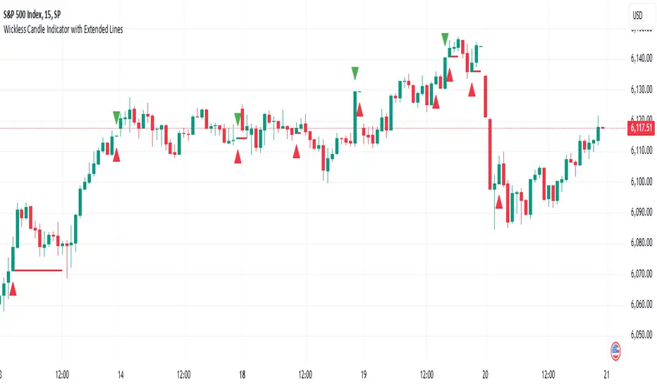
Wickless Candle Indicator with Extended Lines (final)This Pine Script indicator identifies “wickless” candles—those with no upper wick (when the close equals the high) or no lower wick (when the open equals the low)—and marks these events on the chart. When such a candle is detected, it:
Records the Level and Bar Index:
Saves the price level (high for wickless tops, low for wickless bottoms) and the bar index where the condition occurred.
Draws an Extended Horizontal Line:
Creates a green horizontal line for a wickless top or a red line for a wickless bottom, starting at the detection bar and extending across subsequent bars as long as the price remains below (for tops) or above (for bottoms) the recorded level.
Resets When the Price Breaks the Level:
If a future bar’s price moves beyond the saved level (i.e., a high above a wickless top or a low below a wickless bottom), the indicator resets that level, ending the extension of the line.
Visual Markers:
Additionally, it plots a small triangle above a wickless top and below a wickless bottom for easy identification on the chart.
Overall, this script helps traders visualize potential support or resistance levels created by candles that close at their highs or open at their lows, with lines that dynamically adjust as price evolves.
Window Seasonality IndicatorThis is a time window seasonal returns indicator. That is, it will provide the mean returns for a given time window based on a given number of lookbacks set by the user. The script finds matching time windows, e.g., 1st week of March going back 5 years or 9:00-10:00 window of every day going 50 days, and then calculates an average return for that window close price with respect to the close price in the immediately preceding time window, e.g. last week of February or 8:00-9:00 close price, respectively.
There are 4 input options:
1) Historical Periods to Average: Set the number of matching historical windows with which to calculate an average price. The max is 730 lookback windows. Note: for monthly or weekly windows, setting too large a number will cause the script to error out.
2) Use Open Price: calculates the seasonal returns using the open price rather than close price.
3) Show Bands: select from 1 Gaussian standard deviation or a nonparamateric ranked confidence interval. As a rough heuristic, the Gaussian band requires at least 30 lookback periods, and the ranked confidence interval requires 50 or more.
4) Upper Percentile: set the upper cutoff for ranked confidence interval.
5) Lower Percentile: set the lower cutoff for ranked confidence interval.
Please be aware, this indicator does not use rigorous statistical methodology and does not imply predictive power. You'll notice the range bands are very wide. Do not trade solely based on this indicator! Certain time windows, such as weekly and monthly, will make more sense applied to commodities, where annual cycles play a role in its supply and demand dynamics. Hourly windows are more useful in looking at equities markets. I like to look at equities with 1-hr windows to see if there is some pattern to overnight behavior or for market open and close.

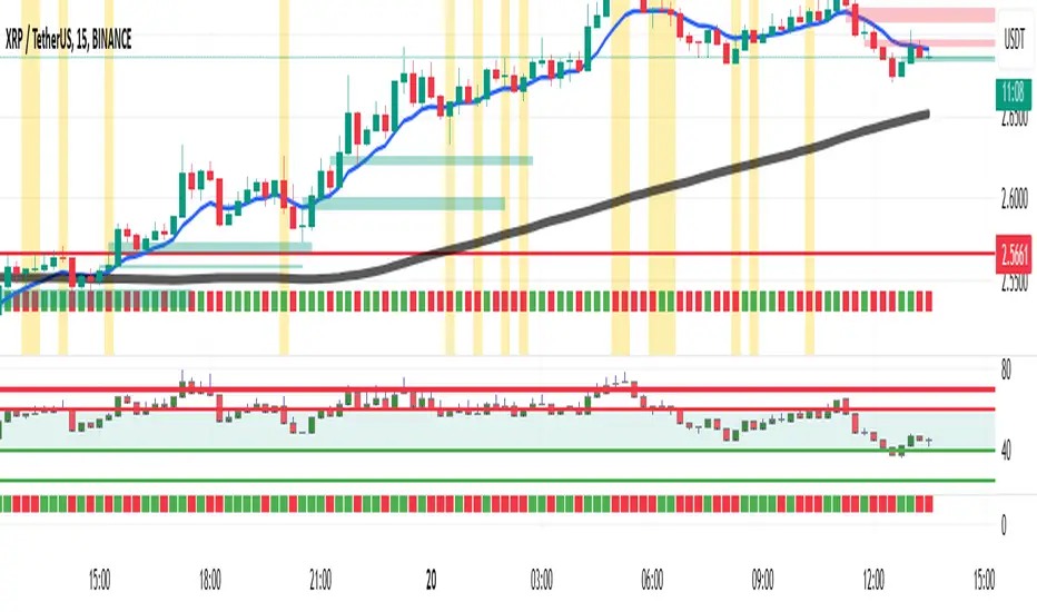
Opposite Delta Candle Highlighter with EMAs & Delta Boxes**Description:**
This indicator is designed to enhance market analysis by highlighting **candles with opposite-colored delta**, plotting **Exponential Moving Averages (EMAs)**, and displaying **delta volume as small boxes below the chart**.
🔹 **Key Features:**
✅ **Opposite Delta Candle Highlighting** – Candles where delta volume contradicts the price direction are highlighted with a **yellow background** and a **blue triangle** above the bar.
✅ **Three Exponential Moving Averages (EMAs)** – Includes **EMA (9, 21, 50)** to help identify trends and dynamic support/resistance levels.
✅ **Delta Volume Display** – Instead of large volume columns, delta is plotted as **small square boxes below the chart**, ensuring clear visibility without overlapping price candles.
✅ **Optimized for Lower Timeframes** – The indicator **automatically selects an appropriate lower timeframe** for more precise delta calculations.
🔹 **How It Works:**
- **Green Candle + Red Delta** → Opposite delta signal (Bearish Sign).
- **Red Candle + Green Delta** → Opposite delta signal (Bullish Sign).
- **Delta bars below the chart** indicate the strength of buying/selling pressure.
- **EMAs help identify the market trend** and potential trade entry zones.
🔹 **Use Cases:**
✔ **Scalping & Day Trading** – Identify potential reversals and trend continuation setups.
✔ **Volume Analysis** – Understand market participation and possible absorption.
✔ **Trend Confirmation** – Use EMAs to confirm trend direction alongside delta volume.
📌 *Best used with lower timeframes (1m, 5m, 15m) for detailed volume analysis.*
🚀 **Enhance your trading with real-time delta insights and price action analysis!**
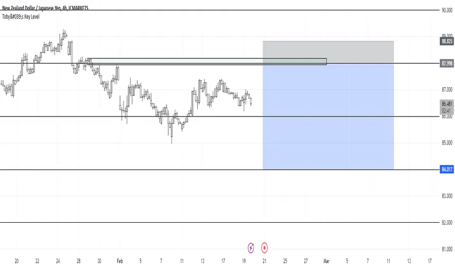
Toby's Key LevelsAn Indicator that helps determine Key Areas on the chart. You set the values you want the horizontal lines to update. They horizontal lines will be used for exits and entries of trade. My recommendation for these Key Areas are as follows ( These recommendations are mostly for day trading and swing trading ):
XAU: Value distance of 50 ex. XAUUSD.
NAS: Value distance of 250 ex. NAS100/USTEC.
ETH: Value distance of 100 ex. ETHUSD.
AUD pairs: Value distance of 0.0200 ex. GBPAUD, EURAUD.
CAD pairs: Value distance of 0.0100 ex. NZDCAD, EURCAD.
CHF pairs: Value distance of 0.0100 ex. CADCHF, GBPCHF.
GBP pairs: Value distance of 0.00350 ex. EURGBP.
JPY pairs: Value distance of 2.00 ex. EURJPY, GBPJPY.
NZD pairs: Value distance of 0.015 ex. GBPNZD, AUDNZD.
Note:
These are subject to change and you can alter the lines anyhow you want to suit your trading style. These are what I recommend. Remember, Market is King.
Safe Trading!
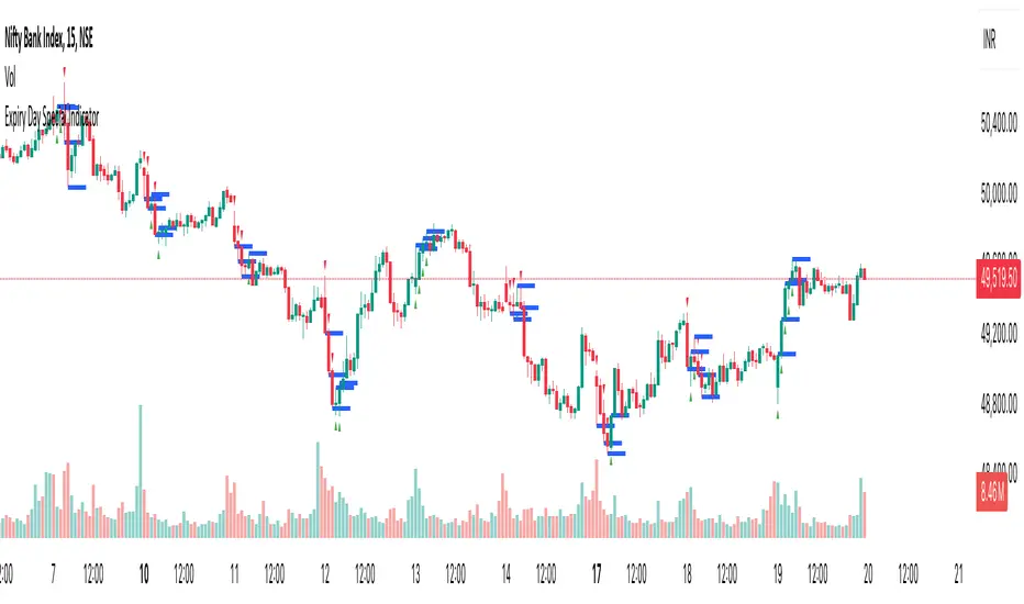
Expiry Day Special IndicatorExpiry Day Special Indicator
The Expiry Day Special Indicator is designed to detect catalytic price action patterns that commonly occur between 9:15 AM to 10:15 AM (IST) in the Nifty & Bank Nifty markets but not limited to these specific markets. While these patterns are particularly useful on expiry days, they are not limited to expiry trading alone. They can also be applied on other trading days when similar conditions arise, making them versatile for intraday traders.
How It Works
This indicator scans for bullish and bearish price action patterns within the first trading hour and plots potential buy and sell signals based on key market structures.
• Bearish Patterns: Identifies strong rejection zones and weakness in price action to signal potential short trades.
• Bullish Patterns: Recognizes reversal formations that indicate potential long trade opportunities.
• Time Filter: The setup is valid only between 9:15 AM - 10:15 AM (IST) to focus on high-impact market moves.
Why This Indicator?
1. Specialized for Nifty & Bank Nifty – Designed specifically for Indian markets.
2. Early Trend Identification – Helps traders capture moves early in the session.
3. Works Beyond Expiry Days – Although optimized for expiry trading, it can also detect similar patterns on regular days.
📌 Note: This indicator does not provide trading advice; always use proper risk management.
Smart Adaptive Signal SystemSmart Adaptive Signal System
Description: The Smart Adaptive Signal System is a sophisticated indicator that generates intelligent buy/sell signals by dynamically adapting to market conditions. It predicts target prices based on momentum and volatility, providing more accurate and reliable trading opportunities.
How It Works:
Dynamic Signal Generation: The system predicts target prices by considering factors such as volatility and momentum. This allows it to react instantly to trend changes and market fluctuations.
Adaptive Thresholds: Buy and sell signals are triggered with adaptive thresholds, adjusting according to market volatility. This ensures flexibility in the face of sudden market changes.
Trend-Based Reset: Users can choose to reset threshold values based on a time interval or trend change. This feature helps the system re-adapt to current market conditions for greater accuracy.
Target Price Prediction: Target prices are calculated using momentum and volatility, helping the system predict future price movements.
How to Use:
Buy/Sell Signals: The indicator generates buy and sell signals based on market conditions. Look for a "down arrow" for a buy signal and an "up arrow" for a sell signal on the chart.
Target Price Lines: Along with buy and sell signals, the system draws target price lines. This helps you visualize potential future price levels.
Flexible Settings: Users can customize analysis periods, minimum change percentages, and other parameters to fit their needs.
Features:
Dynamic buy and sell signals
Target price predictions
Volatility and momentum-based analysis
User-friendly and flexible settings
Trend-based adaptive resetting
Alerts: The Smart Adaptive Signal System responds quickly to sudden market changes, but always use it in conjunction with other indicators like support and resistance levels. Signal accuracy may vary depending on market conditions.
Candle Bias ForecastCandle Bias Forecast Indicator
Description:
The Candle Bias Forecast Indicator is an original multi‐timeframe analysis tool that generates price forecast levels based on the difference between candle biases on two different timeframes. It uses innovative calculations to provide potential forecast levels that align with current price action.
How It Works:
1. Candle Bias Calculation:
For each candle, the indicator computes a “candle bias” using the formula:
candleBias = (((open + close)/2 - (high + low)/2) + ((close - open)/(high - low)))/2
This measure captures both the positioning of the candle’s body within its range and the normalized move from open to close.
2. Multi-Timeframe Analysis:
The script uses multiple timeframe pairs (e.g., 5-minute vs. 30-minute, 10-minute vs. 60-minute, etc.). For each pair, the bias is computed on the lower timeframe and on the higher timeframe.
3. Normalization with ATR:
To translate the dimensionless bias difference into price terms, the indicator multiplies the difference by the lower timeframe’s Average True Range (ATR). This scales the forecast adjustment to current market volatility.
4. Forecast Computation:
The forecast level for each pair is then calculated as:
forecast = close + (lowerTF_ATR * (lowerTF_bias - higherTF_bias))
This yields forecast levels that are plotted on the chart and connected by lines for a visual guide.
How to Use:
- Visual Confirmation: Add the indicator to your 1 to 15 minute chart to see forecast levels overlaid on the price.
- Supplementary Analysis: Use these forecast levels as an additional tool alongside your other analysis methods. They can help indicate potential support/resistance areas or directional bias.
Important Notes:
- Not a Standalone Signal: This indicator is intended to supplement your analysis. Always combine it with other tools and sound risk management practices.
- For Educational & Research Use: The indicator is provided “as is” without any guarantee of performance. It is designed to illustrate an innovative approach to multi-timeframe analysis.
- Disclaimer: Past performance is not indicative of future results. Use this tool at your own risk.
By combining candle bias with ATR-based normalization and multi-timeframe analysis, this indicator offers a unique perspective on market dynamics that can enrich your trading strategy.
---
*This is an original script designed to add value to the TradingView community. Please test and validate its outputs thoroughly before using it in live trading.*

Midnight Range Standard DeviationsCredit to Lex Fx for the basic framework of this script
This indicator is designed to assist traders in identifying potential trading opportunities based on the Intraday Concurrency Technique (ICT) concepts, specifically the midnight range deviations and their relationship to Fibonacci levels. It builds upon the work of Lex-FX, whom we gratefully acknowledge for the original concept and inspiration for this indicator.
Core Concept: ICT Midnight Range
The core of this indicator revolves around the concept of the midnight range. According to ICT, the high and low formed in a specific time window (typically the first 30 minutes after midnight, New York Time) can serve as a key reference point for intraday price action. The indicator identifies this range and projects potential support and resistance levels based on deviations from this range, combined with Fibonacci ratios.
How ICT Uses Midnight Range Deviations
ICT methodology often involves looking for price to move away from the initial midnight range, then return to it, or deviate beyond it, as key areas for potential entries.
Range Identification: The indicator automatically identifies the high and low of the midnight range (00:00 - 00:30 NY Time).
Deviation Levels: The indicator calculates and displays deviation levels based on multiples of the initial midnight range. These levels are often used to identify potential areas of support and resistance, as well as potential targets for price movement. These levels can be set in the additional fib levels section, which can be configured in increments of .5 deviations all the way up to 12 deviations.
Fibonacci Confluence: ICT often emphasizes the confluence of multiple factors. This indicator adds Fibonacci levels to the midnight range deviations. This allows traders to identify areas where Fibonacci retracements or extensions align with the deviation levels, potentially creating stronger areas of support or resistance.
Looking for Sweeps: ICT often uses these levels to look for times that the high and low are swept as potential areas of liquidity, indicating the start of potential continuations.
Time-Based Analysis: The time at which price interacts with these levels can also be significant in ICT. The indicator provides options to extend the range lines to specific times (e.g., 3 hours, 6 hours, 10 hours, 12 hours, or a custom defined time) after midnight, allowing traders to focus on specific periods of the trading day.
Indicator Settings Explained:
Time Zone (TZ): Defines the time zone used for calculating the midnight range. The default is "America/New_York".
Range High Color, Range Low Color, Range Mid Color: Customize the colors of the high, low, and mid-range lines.
Range Fill Color: Sets the fill color for the area between the range high and low.
Line Style: Choose the style of the range lines (solid, dashed, dotted).
Range Line Thickness: Adjust the thickness of the range lines for better visibility.
Show Fibonacci Levels: Enable or disable the display of Fibonacci deviation levels.
Fib Up Color, Fib Down Color: Customize the colors of the Fibonacci levels above (up) and below (down) the midnight range.
Show Trendline: Enables a trendline that plots the close price, colored according to whether the price is above the high, below the low, or within the midnight range.
Show Range Lines, Show Range Labels: Toggles the visibility of the range lines and their associated labels.
Label Size: Adjust the size of the labels for better readability.
Hide Prices: Option to display only the deviation values on labels, hiding price values.
Place Fibonacci Labels on Left Side: Option to switch label position from right side to left side.
Extend Range To (Hours from Midnight): This section gives you a wide variety of options on how far you want to extend the range to, you can do 3,6,10,12, and 23 hours. Alternatively, you can select the "Use Custom Length" and set a specific time in hours.
Additional Fib Levels: This section allows the trader to set additional deviation points in increments of .5 deviations from .5 all the way up to 12 deviations
TradingView Community Guidelines Compliance:
This indicator description adheres to the TradingView community guidelines by:
Being educational: It explains the ICT methodology and how the indicator can be used in trading.
Being transparent: It clearly describes all the indicator's settings and their purpose.
Providing credit: It acknowledges Lex-FX as the original author of the concept.
Avoiding misleading claims: It does not guarantee profits or imply that the indicator is a "holy grail."
Disclaimer: Usage of this indicator and the information provided is at your own risk. The author is not responsible for any losses incurred as a result of using this indicator.
Important Considerations:
This indicator is intended for educational purposes and to assist in applying the ICT methodology.
It should not be used as a standalone trading system.
Always combine this indicator with other forms of technical analysis and risk management techniques.
Backtest thoroughly on your chosen market and timeframe before using in live trading.
Trading involves risk. Only trade with capital you can afford to lose.

Half Candle RetraceThis custom indicator draws a horizontal line at the 50% retracement level of each candlestick on the chart. It calculates the midpoint between the high and low of each candle, which is often used by traders to identify potential entry, exit and take-profit levels. Once price action returns to an untouched level, the line will be removed, leaving only the levels where price action is still missing.
Key Features:
Timeframe: Works on all timeframes.
Line Color: Customize the line color to suit your charting preferences.
Line Width: Adjust the thickness of the retracement line for better visibility.
Line Style: Choose between solid, dotted, or dashed lines.
Up/Down Candle Selection: Option to only display retracement lines for up (bullish) candles, down (bearish) candles, or both.
Full Customization: Control the transparency (opacity) of the line for enhanced visual clarity.
Simple Setup: No complicated settings – simply choose your preferred color, line style, and visibility options.
This indicator is perfect for traders who prefer to use price action and retracement levels to identify potential trade opportunities.
How It Works:
The indicator automatically calculates the 50% level (midpoint) for each candlestick, drawing a line at this level. It will only draw lines for candles that match your chosen criteria (up or down candles), ensuring the chart remains clean and relevant to your trading strategy. Lines are automatically removed as soon as price crosses them.