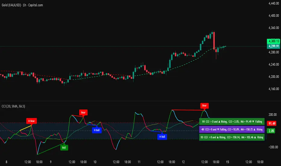
Commodity Channel IndexThe Commodity Channel Index (CCI) is a technical indicator that measures the strength of the momentum in the market, it is calculated using a Moving average (default 20 SMA, users can change the legth and the type of the MA from dashboard) using formula: cci = (src - ma) / (0.015 * ta.dev(src, ccilength)).
When CCI is under -100 that indicates a strong downtrend, and above +100 level a strong uptrend, above 0 level a bullish trend start and bellow 0 level bearish momentum.
Crossing back above -100 and bellow + 100 levels not means it is a reversal of the trend, could be just a pullback or a bounce before trend continuation.
The indicator display on the main chart a color coded moving average with the length and type selected by users for CCI calculation.
The CCI Moving average and the CCI lines in oscillator are both color coded :
1. CCI and MA both red = > Bearish trend
2. CCI and MA both green = > Bullish trend
3. MA color turn yellow or the CCI turn blue that means a possible consolidation will be next or trend change.
4 type of Divergences are detected by the script Bullish, Bearish, Hidden Bullish and Hidden bearish divergences, users can setup alarms for them, by default the divergences ae not displayed, users need to select them to be displayed on the oscillator.
A table displaying the vurrent timeframe and 2 higher timeframes of the stats of CCI and its MA.
There are 13 alerts that users can setup akarms:
Alert for Regular Bullish Divergence
Alert for Hidden Bullish Divergence
Alert for Regular Bearish Divergence
Alert for Hidden Bearish Divergence
Alert for CCI Back Above -100
Alert for CCI Back Bellow 100
Alert for CCI Extreme Overbought
Alert for CCI Extreme Oversold
Alert for trend change by CCI MA => Moving Average Color turned to yellow, that means sideways or possible trend change
Alert for CCI Crossing Above CCI MA
Alert for CCI Crossing Bellow CCI MA
Alert for cci Crossing Above 0
Alert for CCI Crossing Bellow 0
Ortalanmış Osilatörler
3SPC Three Candle Price Action Setup3SPC (Three Candle Price Action Setup) is an open-source indicator designed to detect
a simple and clearly defined three-candle price action pattern.
The logic is based on the following structure:
• The first two candles move in the same direction (bullish or bearish).
• The third candle interacts with the real bodies of both previous candles,
which may indicate a short-term liquidity sweep or price reaction.
• A bullish setup is confirmed when price holds above the open of the first candle.
• A bearish setup is confirmed when price holds below the open of the first candle.
This script does not use oscillators or lagging indicators.
It is intended as a visual aid for discretionary traders and should be used
together with market context, risk management and higher timeframe analysis.
The script is published as open-source for educational and transparency purposes.
UI Labels Translation:
- نمایش ستاپ صعودی: Show bullish setups
- نمایش ستاپ نزولی: Show bearish setups

MTF Trend DashboardThe Multi-Timeframe Trend Dashboard PRO is an advanced technical analysis tool that consolidates trend signals across six configurable timeframes into a single, intuitive heat-map dashboard. Designed for traders who need instant market clarity without switching between charts.
Core Features
🌊 Multi-Timeframe Analysis
Analyzes up to 6 customizable timeframes simultaneously (5m, 15m, 1H, 4H, Daily, Weekly)
Each timeframe independently evaluated for trend direction and strength
Weighted scoring system prioritizes higher timeframe signals
📈 Four-Pillar Technical Confluence
EMA Crossover (20/50) - Trend direction indicator (🟢 Bullish / 🔴 Bearish)
RSI (14) - Momentum analysis with exact values and overbought/oversold zones
MACD (12,26,9) - Momentum confirmation (🟢 Positive / 🔴 Negative)
Volume Analysis - Confirms move validity (🔥 High / ❄️ Low / ⚪ Normal)
🎯 Smart Signal System
🚀 STRONG BUY - All indicators strongly bullish (Score ≥2.5)
📈 BUY - Multiple bullish confirmations (Score 1.5-2.5)
🟢 Bullish - Mild uptrend (Score 0-1.5)
⚪ NEUTRAL - Sideways market (Score = 0)
🔴 Bearish - Mild downtrend (Score -1.5 to 0)
📉 SELL - Multiple bearish confirmations (Score -2.5 to -1.5)
💥 STRONG SELL - All indicators strongly bearish (Score ≤-2.5)
🎨 Heat-Map Color Coding
Bright Green = Strong uptrend with high conviction
Yellow = Neutral/Choppy conditions
Bright Red = Strong downtrend with high conviction
Color intensity reflects signal strength
💪 Strength Meter
Visual bar showing average trend strength across all timeframes (0-100%)
Helps identify powerful moves vs weak consolidations
🎯 Overall Bias
Weighted composite score emphasizing higher timeframes
Daily/Weekly signals carry 4-5x more weight than intraday
Provides "big picture" directional bias
🚨 Built-in Alert System
Strong Bullish/Bearish Confluence detected
Major trend changes across multiple timeframes
Customizable alert messages
How to Use
Trend Confirmation - Look for alignment (all rows showing same color = strong trend)
Divergence Detection - Lower timeframes differ from higher = potential reversal
Entry Timing - Wait for Overall Bias + multiple green signals with 🔥 volume
Risk Management - Avoid trades when Overall Bias shows ⚪ NEUTRAL
Customization
Adjustable EMA, RSI, MACD, Volume parameters
Flexible timeframe selection (enable/disable any TF)
Dark/Light theme support
Position and size controls
© | Built on TradingView
Precision tools for precision traders.

VEGA (Velocity of Efficient Gain Adaptation)VEGA (Velocity of Efficient Gain Adaptation)
VEGA is a momentum oscillator that measures the velocity of an efficiency-weighted adaptive moving average. Unlike traditional momentum indicators that react uniformly to all price movements, VEGA intelligently adapts its sensitivity based on market conditions—responding quickly during trending periods and filtering noise during consolidation.
--------------------------------
What Makes VEGA Different
Efficiency-Driven Adaptation
At its core, VEGA uses the Efficiency Ratio (ER) to distinguish between trending and choppy markets. When price moves efficiently in one direction, VEGA's underlying adaptive MA speeds up to capture the move. When price chops sideways, it slows down to avoid whipsaws. This creates a momentum reading that's inherently cleaner than fixed-period alternatives.
Linear Regression Smoothed Source
VEGA offers an optional LinReg-smoothed price source that blends regular candles with linear regression values. This pre-smoothing reduces noise before it ever enters the calculation, resulting in a histogram that's easier to read without sacrificing responsiveness. The mix ratio lets you dial in exactly how much smoothing you want.
Z-Score Normalization with Dead Zone
Rather than arbitrary oscillator bounds, VEGA normalizes output as standard deviations from the mean. This gives statistically meaningful levels: readings above +2σ or below -2σ represent genuinely extreme momentum. The configurable dead zone (with Snap, Soft Fade, or None modes) filters out insignificant movements near zero, keeping you focused on signals that matter.
--------------------------------
How It Works
1. Source Preparation — Price is smoothed via a LinReg/regular candle blend
2. Efficiency Ratio — Measures directional movement vs total movement over the lookback period
3. Adaptive MA — Applies variable smoothing based on efficiency (fast during trends, slow during chop)
4. Velocity — Calculates the rate of change of the adaptive MA
5. Normalization — Converts to Z-Score (standard deviations) or ATR-normalized percentage
6. Dead Zone — Optionally filters near-zero values to reduce noise
--------------------------------
How To Read VEGA
Signal and Interpretation
Histogram above zero | Bullish momentum
Histogram below zero | Bearish momentum
Bright color | Momentum accelerating
Faded color | Momentum decelerating
Beyond ±1σ bands | Above-average momentum
Beyond ±2σ bands | Extreme momentum (potential reversal zone)
Zero line cross*| Momentum shift
--------------------------------
Key Settings
ER Length — Lookback for efficiency ratio calculation. Higher = smoother, slower adaptation.
Fast/Slow Smoothing — Controls the adaptive MA's responsiveness range. The MA blends between these based on efficiency.
LinReg Settings — Enable smoothed candles and adjust the blend ratio (0 = regular candles, 1 = full LinReg, 0.5 = 50/50 mix).
Z-Score Lookback — Period for calculating mean and standard deviation. Shorter = more reactive normalization.
Dead Zone Type — How to handle near-zero values:
Snap — Hard cutoff to zero
Soft Fade — Gradual reduction toward zero
None — No filtering
Dead Zone Threshold — Values within this Z-Score range are affected by the dead zone setting.
VEGA works on any timeframe and any market. For best results, adjust the ER Length and LinReg settings to match your trading style and the volatility characteristics of your instrument.

Beast Mode PRO v4.0# Beast Mode PRO v4.0 - Advanced Multi-Regime Trading System
## Overview
Beast Mode PRO v4.0 is a sophisticated technical analysis indicator designed for active traders seeking high-probability setups across multiple timeframes. This system combines machine learning-inspired clustering algorithms with traditional technical analysis to identify market regimes and generate precision entry signals. The indicator adapts to different trading styles through intelligent preset configurations and multiple trading modes.
---
## Core Methodology
### Signal Generation Framework
The indicator employs a **multi-component voting system** that analyzes market conditions through several independent technical perspectives:
**Technical Components:**
- **RSI (Relative Strength Index)**: Momentum oscillator measuring overbought/oversold conditions
- **Fisher Transform**: Price transformation technique that normalizes price distributions for clearer turning points
- **DMI (Directional Movement Index)**: Trend strength indicator measuring directional pressure
- **Z-Score Analysis**: Statistical measure identifying price deviations from historical norms
- **Moving Average Ratio**: Price relationship to its moving average baseline
- **MFI (Money Flow Index)**: Volume-weighted momentum indicator
- **Stochastic Oscillator**: Momentum indicator comparing closing price to price range
- **CCI (Commodity Channel Index)**: Measures current price level relative to average price level
### Clustering Engine
The system utilizes a **k-means inspired clustering algorithm** that categorizes each technical indicator's normalized values into distinct market regimes (bullish, bearish, neutral). This approach:
1. **Normalizes** all indicators using z-score transformation over a historical lookback window
2. **Clusters** normalized values using percentile-based thresholds
3. **Aggregates** individual votes into a composite score ranging from -100 to +100
4. **Smooths** the composite score using selectable methods (SMA, EMA, WMA, HMA, TEMA, DEMA)
The clustering percentiles adapt dynamically based on current market volatility (ATR-normalized), ensuring the system remains responsive across different market conditions.
---
## Trading Modes
### 1. Normal Mode
Standard crossover-based signals using fixed thresholds (+10/-10). Suitable for balanced trading with moderate signal frequency.
### 2. Scalper Mode
Dynamic threshold adjustment based on recent score volatility. Generates more frequent signals by adapting to short-term price movements.
### 3. Aggressive Mode
Reversal-focused approach that triggers signals when the composite score crosses extreme levels (+80/-80), targeting major trend reversals.
### 4. Hybrid Mode
Combines Normal and Aggressive signals, capturing both standard crossovers and extreme reversals for comprehensive market coverage.
### 5. Super Scalper Mode
Ultra-responsive mode using signal line crossovers (14-period HMA of composite score) for maximum trade frequency.
### 6. Sniper Mode (Premium Feature)
Multi-confirmation system requiring alignment of:
- Composite score threshold breach
- Positive fast momentum (10-period SMI)
- Positive trend momentum (200-period SMI)
- Price above/below smart trend filter MA
This mode prioritizes precision over frequency, filtering out low-probability setups.
---
## Timeframe Presets
Pre-optimized configurations for common trading timeframes:
### 1 Minute Preset
- Fast smoothing (10-period WMA)
- Tight chop filter (61.8 threshold)
- Optimized for rapid scalping with minimal lag
### 2 Minute Preset
- Balanced smoothing (12-period EMA)
- Enhanced volume filtering
- Moderate cooling period (5 bars)
### 3 Minute Preset
- HMA smoothing for reduced lag
- Stochastic and CCI enabled
- Balanced approach for intraday trading
### 5 Minute Preset
- TEMA smoothing for trend following
- Stronger filters to reduce noise
- Extended lookback (1000 bars)
### 15 Minute Preset
- DEMA smoothing for swing positions
- Maximum filtering configuration
- All technical indicators enabled
- Suitable for swing trading and position building
Users can also select "Custom" to manually configure all parameters.
---
## Advanced Filtering System
### 1. Choppy Market Filter
Uses Choppiness Index calculation to identify consolidating markets. When CI exceeds the threshold, signals are suppressed to avoid whipsaw trades.
### 2. Smart Trend Filter
Configurable moving average (SMA/EMA/WMA/HMA/TEMA/DEMA/VWMA/RMA) that prevents counter-trend signals. Long signals require price above the MA, shorts require price below.
### 3. Volume Filter
Compares current volume to its moving average. Signals are suppressed when volume falls below the specified multiplier of average volume.
### 4. ATR Volatility Filter
Prevents trading during low volatility periods when ATR falls below its moving average multiplied by the specified factor.
### 5. Session Filter
Time-based filtering for Asia, London, New York, or combined sessions. Ensures trading only during preferred market hours.
### 6. Multi-Timeframe Confirmation
Optionally requires higher timeframe alignment before generating signals, adding confluence for higher probability trades.
### 7. Cooling Off Period
Prevents signal clustering by enforcing a minimum number of bars between consecutive signals.
---
## Smart Money Concepts Integration
### Order Block Detection
Identifies institutional supply/demand zones using multi-timeframe analysis:
- Detects strong directional candles followed by breakout moves
- Volume confirmation ensures significance
- Customizable timeframe selection (current TF or higher TF: 5m, 15m, 30m, 1H, Daily)
- Visual boxes mark active order blocks with automatic expiration after lookback period
- Price interaction alerts when touching active zones
### Liquidity Zones
Marks equal highs (EQH) and equal lows (EQL) where stop losses typically cluster, indicating potential reversal or breakout points.
---
## Momentum Analysis
### Fast Momentum (Default: 10-period)
Short-term momentum oscillator using Stochastic Momentum Index (SMI) calculation. Provides early warning of momentum shifts.
### Trend Momentum (Default: 200-period)
Long-term momentum gauge confirming overall trend direction. Used in Sniper Mode for multi-confirmation.
### Momentum Divergence Detection
Automatically identifies:
- **Regular Divergence**: Price makes new high/low but momentum doesn't (reversal signal)
- **Hidden Divergence**: Price makes higher low/lower high but momentum doesn't (continuation signal)
---
## Visual Components
### Price Chart Overlay
- **Smart Trend MA**: Dynamically colored moving average based on price position
- **EMA Cloud**: 50/200 EMA cloud showing long-term trend (background shading)
- **Trend Background**: Subtle background coloring based on composite score
- **Order Block Boxes**: Institutional supply/demand zones
- **Entry/Exit Markers**: Clear visual signals with emoji labels
- **Liquidity Markers**: EQH/EQL identification
### Bar Coloring
Bars change color based on active mode and market regime:
- **Sniper Mode**: Purple (bull) / Pink (bear)
- **Aggressive Mode**: Bright Green / Bright Red
- **Super Scalper**: Neon Green / Neon Red
- **Timeframe Presets**: Unique color schemes per preset
- **Choppy/Neutral**: Always gray regardless of mode
### Oscillator Pane
- **Composite Score Line**: Gradient-colored stepline showing current regime strength
- **Fast/Trend Momentum**: Optional overlays (gold/cyan colors)
- **Divergence Markers**: Visual alerts for regular, hidden, and momentum divergences
- **Power Zones**: Overbought/oversold regions (80/-80 levels)
- **Dynamic/Fixed Thresholds**: Visual reference lines based on active mode
### Interactive Dashboards
**Main Dashboard** displays:
- Active preset/mode configuration
- Real-time indicator values and votes
- Current market status (active/choppy/counter-trend/low volume/low ATR/MTF misalignment)
- Regime classification (Strong Long/Long/Neutral/Short/Strong Short)
- Smart Trend MA status
**Performance Dashboard** shows:
- Exit strategy (Fixed TP/SL, Trailing Stop, Opposite Signal)
- Total trades and win rate
- Total points and average per NY session
- Profit factor and recovery factor
- Best/worst trades and max drawdown
- Maximum winning/losing streaks
- Sharpe ratio and average risk:reward
**TP Optimizer** (33 variations tested):
- Tests take profit levels from 40 to 200 ticks (5-tick increments)
- Sortable by: Profit Factor, Win Rate, Total Points, Sharpe Ratio
- Displays top 5 configurations with full metrics
- Real-time optimization during backtesting
---
## Backtest Engine
### Exit Strategies
**1. Fixed TP/SL**
- Configurable in Ticks, ATR multiples, or Percentage
- Precise risk management with predefined targets
**2. Exit on Opposite Signal**
- Closes position when counter-signal appears
- Adapts to changing market conditions
- Useful for trend-following approaches
**3. Trailing Stop**
- Dynamic stop loss that follows profitable moves
- Configurable trailing offset percentage
- Locks in profits while allowing trends to develop
### Risk Management
- Optional minimum risk:reward filter
- Prevents trades below specified R:R threshold
- Date range filtering for historical analysis
- Session-based performance tracking
### Performance Metrics
- Win rate, profit factor, Sharpe ratio
- Maximum drawdown and recovery factor
- Consecutive win/loss streaks
- Average win/loss analysis
- Gross profit vs gross loss breakdown
---
## Alert System
Comprehensive alert conditions for:
- Entry signals (Long/Short)
- Exit events (TP/SL/Opposite/Trailing)
- Trend signals (Strong bullish/bearish)
- Divergences (Regular/Hidden/Momentum)
- Order block detection and touches
- Multi-condition strong signals (all confirmations aligned)
---
## How to Use
### Quick Start
1. Select your preferred timeframe preset (1m, 2m, 3m, 5m, 15m, or Custom)
2. Choose a trading mode (Normal, Scalper, Aggressive, Hybrid, Super Scalper, or Sniper)
3. Configure session filter to match your trading hours
4. Enable desired filters (choppy, trend, volume, ATR, MTF)
5. Set your exit strategy and TP/SL levels
6. Monitor signals on price chart and oscillator pane
### Optimization Workflow
1. Enable "Run TP Optimizer" in backtest settings
2. Run backtest on historical data
3. Review Optimizer Dashboard for best TP levels
4. Sort by preferred metric (Profit Factor, Win Rate, Total Points, Sharpe)
5. Apply winning configuration to live trading
### Advanced Configuration
- Customize individual indicator lengths and enable/disable specific components
- Adjust clustering parameters (lookback window, percentiles, cluster count)
- Fine-tune smoothing methods and lengths
- Configure order block detection timeframe and sensitivity
- Set cooling off period to control signal frequency
---
## Unique Features
1. **Adaptive Clustering**: Volatility-adjusted percentiles ensure consistent performance across market conditions
2. **Multi-Mode Architecture**: Six distinct trading modes from conservative to ultra-aggressive
3. **Timeframe Intelligence**: Pre-optimized presets eliminate guesswork for common timeframes
4. **Smart Money Integration**: Order block detection and liquidity zone marking
5. **Comprehensive Backtesting**: Three exit strategies with 33-variation TP optimization
6. **Visual Clarity**: Mode-specific bar coloring and clean chart presentation
7. **Filter Stack**: Seven-layer filtering system prevents low-quality signals
8. **Real-Time Metrics**: Live performance tracking with advanced statistics
---
## Benefits
- **Reduced False Signals**: Multi-confirmation clustering approach filters noise
- **Adaptability**: Works across timeframes and market conditions through preset system
- **Transparency**: Open visualization of all component votes and filtering status
- **Risk Management**: Built-in TP/SL optimization and R:R filtering
- **Time Efficiency**: Preset configurations save hours of manual optimization
- **Educational Value**: Dashboard shows exactly why signals trigger or get filtered
- **Professional Tools**: Institutional concepts (order blocks, liquidity zones) accessible to retail traders
---
## Best Practices
- Use Sniper Mode for high-probability setups during volatile markets
- Enable choppy filter during consolidation periods
- Combine Smart Trend Filter with MTF confirmation for swing trades
- Run TP Optimizer monthly to adapt to changing market dynamics
- Monitor Sharpe Ratio in addition to win rate for risk-adjusted performance
- Use session filters to avoid low-liquidity hours
- Start with preset configurations before custom optimization
---
## Technical Requirements
- TradingView Premium/Pro/Pro+ for full feature access
- Minimum chart history: 500 bars (adjustable in clustering settings)
- Works on all instruments (stocks, forex, crypto, futures)
- Compatible with standard candles (Heikin Ashi optional but not recommended for backtesting)
---
## Disclaimer
This indicator is a technical analysis tool designed to assist trading decisions. It does not guarantee profits and should be used in conjunction with proper risk management, fundamental analysis, and personal trading experience. Past performance does not indicate future results. Users should thoroughly test the indicator on demo accounts before live trading.
---
**Version**: 4.0
**Language**: Pine Script v6
**Type**: Overlay Indicator with Oscillator Pane
**Calculation**: On bar close (default) or real-time (configurable)

SB - RSI EW OscillatorAdd EW with RSI.
Makes sense take a call if RSI is above 50 and EW turns green and vice versa.


Take Profit XTake Profit X
Take Profit X solves the #1 problem in trading: knowing when to exit. Instead of guessing or using single indicators, it aggregates 8 technical signals to identify high-probability exit points through multi-confirmation consensus. This eliminates premature exits and emotional decision-making.
The indicator counts confirmations from your chosen technical tools:
Green dot = Multiple signals say "take profit on longs/exit shorts"
Red dot = Multiple signals say "take profit on shorts/exit longs"
Signals appear when you reach the minimum confirmations threshold you set.
Possible Settings:
Conservative (Swing Trading)
pine
Minimum Confirmations: 4
Use: RSI, MACD, CCI, Supertrend, Price Action
Disable: Stochastic, Bollinger Bands, EMA Cross
Look Back Bars: 10
Aggressive (Day Trading)
pine
Minimum Confirmations: 2
Use: All indicators ON
Look Back Bars: 3-5
RSI OB/OS: 75/25
Balanced (Most Markets)
pine
Minimum Confirmations: 3
Use: RSI, MACD, CCI, Supertrend
Price Action: ON
Look Back Bars: 5-7

Ultimate Adaptive RSIUltimate Adaptive RSI
RSI That Adapts to Any Market
This isn't your grandpa's RSI. It dynamically adjusts its sensitivity based on market conditions—smoother in trends, responsive in ranges.
Traditional RSI fails in strong trends and changing volatility. UA-RSI fixes both by adapting its sensitivity in real-time, giving you reliable signals whether the market is trending, ranging, or transitioning between regimes.
How It Adapts:
Smart Pre-Smoothing: Uses Efficiency Ratio to detect trend strength and automatically lengthens/shortens its smoothing window.
Dominant Cycle Detection: Matches its internal period to the market's actual rhythm.
Dynamic Bands: RMS-based overbought/oversold levels that expand/contract with volatility.
Smoothing Stack: ALMA pre-smoothing → Ultimate Smoother → Jurik filter creates the cleanest RSI you've ever seen.
Trade Signals:
Buy: RSI crosses above lower band or midline + price confirms
Sell: RSI crosses below upper band or midline + price confirms
Bands expand in high volatility → wait for deeper extremes
Bands contract in low volatility → take earlier signals
Signal line for crossover entries
Adaptive smoothing = fewer false signals in trends
Day trading: Use 1.0 band multiplier
Swing trading: Use 1.2-1.5 multiplier
Ranging markets: Lower multiplier to 0.8
Trending markets: Raise multiplier to 1.5+
Bands widen in volatility = wait for deeper extremes
Bands tighten in calm markets = take earlier signals
Never trade RSI alone - always wait for price confirmation

Hybrid Confluence (RSI,MFI,StochRSI) Two-Tier Momentum Framework
Many traders explore multi-oscillator hybrid confluence approaches that combine momentum and volume signals—most commonly RSI, Money Flow Index (MFI), and Stochastic RSI—to study stretched market conditions. These hybrid concepts are widely used to analyze potential exhaustion zones, cycle extremes, and periods of sustained buying or selling pressure across different timeframes.
This script does not replicate, reverse-engineer, or replace any paid or closed-source indicator.
Instead, it provides a fully transparent framework built exclusively from standard, well-documented technical indicators. All calculations are explicit and configurable, allowing traders to study hybrid momentum behavior without relying on proprietary logic or black-box tools.
What the Script Does
1. Builds a hybrid momentum confluence model
The script combines three widely used oscillators:
• RSI (Relative Strength Index) — price momentum
• MFI (Money Flow Index) — volume-weighted momentum
• Stochastic RSI — momentum relative to its own recent range
Each component operates on a normalized 0–100 scale, allowing meaningful comparison and aggregation.
2. Implements a clear two-tier signal structure
Instead of producing a single binary buy/sell output, the script separates early pressure from extreme conditions:
2-of-3 Confluence (Setups)
When any two of the three oscillators reach oversold or overbought levels:
• Displayed as semi-transparent circles
• Indicates building pressure or a developing condition
• Designed as a heads-up, not a trade signal
3-of-3 Confluence (Signals)
When all three oscillators reach oversold or overbought levels:
• Displayed as prominent vertical bars spanning the oscillator range
• Represents extreme momentum alignment
• Intended to highlight potential exhaustion zones
3. Visualizes sustained pressure using consecutive signal intensity
When 3-of-3 conditions persist across multiple bars:
• Each consecutive bar becomes progressively darker
• Up to six discrete intensity levels
• Darkness reflects duration and persistence, not prediction
This helps visualize scenarios where markets continue pushing higher or lower before a major turning point, rather than assuming a single signal marks the exact top or bottom.
4. Works across markets and timeframes
Because all inputs rely on standard technical indicators:
• Works on crypto, equities, futures, and FX
• Scales naturally from intraday to higher timeframes
• Can be used on Daily and multi-day charts for macro context
Why This Script Is Useful
Traditional oscillators often produce isolated signals that lack context. This framework adds clarity by:
1. Requiring multi-indicator agreement instead of single-signal triggers
2. Separating early pressure from extreme conditions
3. Showing how momentum can persist before a reversal
4. Avoiding binary “buy now / sell now” outputs
5. Remaining transparent and configurable
This makes the tool especially useful for:
• Swing traders
• Macro and cycle-focused traders
• Crypto traders studying extended momentum phases
• Analysts who prefer contextual signals over rigid rules
How to Use
1. Adjust RSI, MFI, and StochRSI lengths to suit your timeframe
2. Observe 2-of-3 circles as early warnings of building pressure
3. Watch 3-of-3 bars for extreme momentum alignment
4. Note increasing bar intensity as pressure persists
5. Combine with structure, trend, volume, or price action for decisions
This script is best used as a contextual tool, not a standalone trading system.
What This Script Is Not
• Not a recreation of any paid or proprietary indicator
• Not affiliated with any trading educator or platform
• Not intended as a predictive or standalone trading system
• Does not claim to identify exact tops or bottoms
All signals are derived solely from openly documented RSI, MFI, and Stochastic RSI calculations.
Important Notes
• This script is original, with a transparent methodology
• All calculations use standard, well-known technical formulas
• No hidden logic or undisclosed weighting is used
• Signal visuals are descriptive, not predictive
Disclaimer
This tool is provided for educational and analytical purposes only.
It does not constitute financial advice or a recommendation to trade.
Always validate settings, test on multiple assets and timeframes, and use proper risk management before trading live.

VixTrixVixTrix - Because markets move in both directions.
VixTrix was born from a fundamental limitation in traditional volatility indicators: they only measure downside panic, completely missing the greed-driven extremes that form market tops.
How It Works:
Dual-Component Analysis:
vixBear = Panic selling intensity (distance from recent highs)
vixBull = FOMO buying intensity (distance from recent lows)
Oscillator = vixBear - vixBull = Net fear/greed imbalance
When the oscillator is positive, fear dominates (potential bottom forming). When negative, greed dominates (potential top forming).
Professional-Grade Filtering:
The magic happens with the symmetric RMS (Root Mean Square) bands. Unlike fixed percentage bands or standard deviation, RMS:
Creates mathematically symmetric positive/negative thresholds
Naturally adapts to changing volatility regimes
Provides statistical significance to extremes
VixTrix also adds selectable MA smoothing for the RMS calculation:
WMA (default): Balanced – middle-ground approach
VWMA: Volume-weighted – filters low-volume noise
EMA: Responsive – catches quick reversals
SMA: Stable – for swing trading
HMA: Fast and smooth – ideal for day trading
Signals require triple confirmation:
Statistical Extreme: Oscillator beyond RMS band
Price Action Confirmation: Correct candle color (bullish for bottoms, bearish for tops)
Momentum Continuation: Oscillator still moving toward extreme (exhaustion)
This multi-filter approach reduces premature entries and false signals while maintaining early positioning at potential reversal points.
Why This Matters for Your Trading:
In bull markets, traditional fear indicators sit near zero, giving no warning of impending tops.
VixTrix identifies when greed becomes excessive – when FOMO buying reaches statistical extremes that often precede corrections.
In range-bound markets, VixTrix excels at identifying overreactions in both directions, providing high-probability mean reversion opportunities.
During crashes, it captures the panic selling with the same precision as VixFix, but with better timing through its momentum confirmation.
VixTrix spots continuations through:
"No Signal" = Healthy Trend – Oscillator stays between RMS bands (no exhaustion)
Failed Extremes – Touches band but no triple confirmation = trend likely continues
Hidden Divergence – Price makes higher low while oscillator makes shallower low = uptrend continues
Controlled Emotions – Oscillator negative but not extreme in uptrends (greed present but not excessive)
Key Insight: When VixTrix doesn't give a signal during a pullback, institutions aren't panicking – they're just pausing before resuming the trend.
Green columns = Bullish exhaustion (potential bottoms)
Red columns = Bearish exhaustion (potential tops)
Golden RMS bands = Dynamic thresholds adapting to current volatility
Background highlights = Active signal conditions
The Result: A professional-grade oscillator that works in all market conditions – trending up, trending down, or ranging – by measuring the complete emotional spectrum driving price action.
DeltaPulseDeltaPulse: Professional Cumulative Volume Delta Indicator
DeltaPulse is a free cumulative volume delta (CVD) indicator engineered for modern traders who demand precision, adaptability, and visual clarity. Unlike traditional CVD tools that often suffer from scaling issues, excessive noise, or poor responsiveness across timeframes, DeltaPulse delivers a streamlined, professional-grade solution that "just works" – providing actionable insights into buying and selling pressure with minimal setup.
This indicator accumulates the net difference between buying and selling volume (inferred from candle direction), normalizes it intelligently for consistent readability, and applies advanced smoothing to filter out market noise while preserving momentum signals. The result is a clean, momentum-colored line in a dedicated pane, enhanced by subtle visual cues that highlight key market dynamics.
Whether you're a day trader scalping intraday moves, a swing trader analyzing weekly trends, or an institutional analyst reviewing futures contracts, DeltaPulse adapts seamlessly to your workflow. It's designed to be your go-to tool for confirming trends, spotting divergences, and identifying order flow imbalances – all without the bloat of overcomplicated features.
Key Features
Intelligent Normalization for Universal Compatibility
Automatically adjusts scaling based on chart timeframe and symbol volume profile.
Intraday (1-5 min): Uses a 100-period volume average for responsive, lively signals.
Intraday (15+ min): 50-period average for balanced sensitivity.
Daily/Weekly+: 20-period average for clean, long-term perspective.
Ensures the indicator remains visually meaningful and non-flat on any asset – from low-volume penny stocks to high-liquidity indices like ES or NQ.
Advanced Smoothing Options
Six moving averages to match your trading style:
EMA - Quick reactions to recent delta shifts
SMA - Simple Moving Average - Stable, noise-resistant baseline
WMA - Weighted Moving Average - Emphasizes recent data with linear weighting
HMA - Hull Moving Average - Ultra-smooth yet lag-free – ideal for momentum trading
RMA - Running Moving Average (Wilder's) - Trend-following with minimal whipsaws
VWMA - Volume-Weighted Moving Average - Highlights high-volume delta moves
Lower values increase reactivity; higher values enhance smoothness.
Flexible Reset Mechanisms
Session Reset: Clears CVD at the first regular trading bar each day – perfect for intraday analysis.
Weekly Reset: Resets at the start of each new week – suited for swing and position trading.
No manual intervention required; the indicator handles resets reliably across all timeframes.
Background Shading:
Light green tint above zero; light red below.
Extreme highlights when smoothed CVD exceeds 90% of its 80-bar high/low – flags potential exhaustion or absorption zones.
How It Works
DeltaPulse calculates a simple yet effective volume delta on each bar:
Bullish Bar (close ≥ open): Adds full volume as positive delta.
Bearish Bar (close < open): Subtracts full volume as negative delta.
This raw delta accumulates into a running total (CVD), resetting based on your chosen mode. The total is then:
Normalized against a timeframe-adaptive volume average to ensure consistent scaling.
Smoothed using your selected MA type for noise reduction and trend clarity.
Plotted with momentum-based coloring and visual enhancements.
The output is a single, intuitive line that reveals the underlying battle between buyers and sellers – far more reliably than raw volume bars or basic oscillators.
Trading Applications
DeltaPulse shines in revealing order flow dynamics that price action alone often conceals. Here are proven ways to integrate it:
Trend Confirmation & Momentum Trading
Bullish Setup: Rising green line above zero confirms buyer control – enter longs on pullbacks to support.
Bearish Setup: Falling red line below zero signals seller dominance – short on rallies to resistance.
Zero Line Crosses as Reversal Signals
A crossover from negative to positive territory often marks a sentiment shift – use for entry triggers.
Combine with volume spikes or key levels for high-probability setups.
Enhancement: VWMA mode amplifies signals on high-volume breakouts.
Absorption & Exhaustion Zones
Watch for extreme background highlights: A spike to highs followed by reversal suggests large players absorbing supply.
Ideal for fade trades near overextended levels (e.g., after news events).
Avoid low-volume or illiquid symbols, as delta inference relies on reliable candle data.
Timeframe-Agnostic: Solves the common CVD pitfall of being "dead" on intraday charts or erratic on daily ones through smart, automatic normalization.
Lag-Free Responsiveness: The default HMA smoothing strikes a rare balance – smoother than EMA, faster than SMA – without the computational overhead of exotic filters.
Zero Clutter: No histograms, no extraneous plots, no overwhelming alerts. Just pure, distilled order flow intelligence.

MACD Nexus Pro [OXE]MACD Nexus Pro
Institutional-Grade Momentum Intelligence System
Transform How You Read Market Momentum
Standard MACD indicators show you what happened. MACD Nexus Pro shows you what's about to happen.
Built for serious traders who demand more than basic crossovers, this indicator combines 8 proprietary analysis engines into one powerful momentum intelligence system. Whether you trade forex, crypto, stocks, or commodities — MACD Nexus Pro gives you the institutional edge.
What Makes This Different?
Most MACD indicators are stuck in the 1970s. They show you two lines, a histogram, and leave you guessing. MACD Nexus Pro was engineered from the ground up to answer the questions professional traders actually ask:
"Is this signal confirmed across multiple timeframes?"
"Is this momentum move real or a fake-out?"
"Are smart money players accumulating or distributing?"
"Is this trend exhausted or just getting started?"
Core Benefits for Traders
🎯 Eliminate False Signals with MTF Confluence
Stop getting chopped up by single-timeframe noise. The Multi-Timeframe Confluence Matrix scans 4 timeframes simultaneously and calculates a unified alignment score from -5 to +5.
How it helps you:
Only take trades when multiple timeframes agree
See instantly if higher timeframes support your entry
Avoid counter-trend trades that fail 80% of the time
Build confidence knowing the "big picture" backs your trade
📊 Know Your Market Regime Instantly
Markets behave differently in trending vs ranging conditions. The Regime Detection Engine automatically classifies current conditions as TRENDING, VOLATILE, RANGING, or NEUTRAL.
How it helps you:
Adjust your strategy to match market conditions
Avoid momentum trades in choppy, ranging markets
Capitalize on trending markets with confidence
Stop forcing trades when conditions don't favor your style
🔄 Catch Reversals Early with Smart Divergence Detection
Divergences signal potential reversals before they happen — but spotting them manually is tedious and error-prone. The Divergence Engine automatically detects both Regular and Hidden divergences, then rates their strength.
How it helps you:
Get early warning of trend exhaustion
Find high-probability reversal entries
Use Hidden divergences for trend continuation trades
Prioritize strong divergences (★★★★) over weak ones
🏦 Trade Alongside Smart Money
Institutional players leave footprints. The Smart Money Momentum Zones detect when volume-weighted momentum enters extreme territory — signaling potential accumulation (buying) or distribution (selling) by large players.
How it helps you:
Identify where institutions are likely positioning
Buy in accumulation zones with smart money
Sell or short in distribution zones
Avoid buying into institutional selling
⚡ Distinguish Impulse Moves from Corrections
Not all momentum is created equal. The Impulse Wave Detection system identifies whether current momentum is an impulse (strong, directional) or a correction (weak, counter-trend).
How it helps you:
Enter on impulses, not corrections
Hold winners through corrections without panic
Recognize when a trend is resuming
Time entries at the start of new momentum waves
📍 Never Miss True Equilibrium
Static zero lines are outdated. The Dynamic Zero Line adapts to the market's true momentum equilibrium, shifting based on long-term bias.
How it helps you:
Understand the market's real neutral point
Recognize bullish/bearish bias at a glance
Better time zero-line crossover trades
Filter signals based on positioning above/below equilibrium
⚠️ Get Warned Before Momentum Dies
Chasing extended moves is how traders lose money. The Momentum Exhaustion Detector calculates the thrust-to-follow-through ratio and warns you when momentum is overextended.
How it helps you:
Avoid late entries into tired trends
Take profits before reversals hit
Spot when bulls/bears are running out of steam
Stay patient for better entries after exhaustion
🌈 Read Momentum Strength at a Glance
The Gradient Histogram Heatmap shows momentum acceleration through color intensity — brighter colors mean momentum is building, faded colors mean it's dying.
How it helps you:
Instantly see if momentum is accelerating or fading
Confirm breakouts with strengthening momentum
Spot weakening moves before price confirms
Make faster decisions with visual clarity
The Signal System You Can Trust
Every buy/sell signal comes with a Star Rating (★ to ★★★★★) based on:
Multi-timeframe alignment
Position relative to dynamic zero
Market regime confirmation
Volume confirmation
Exhaustion status
Choose your signal mode:
Standard: Classic MACD crossovers
Confluence: Only signals with MTF agreement (recommended)
Aggressive: Early entries with directional confluence
All signals are 100% non-repainting — what you see is what happened, permanently.
Two Professional Dashboards
MTF Confluence Panel (Top-Right)
TimeframeTrendAbove ZeroCurrent▲/▼✓/✗15min▲/▼✓/✗1H▲/▼✓/✗4H▲/▼✓/✗Daily▲/▼✓/✗
Nexus Status Panel (Bottom-Right)
Regime: TRENDING / VOLATILE / RANGING / NEUTRAL
Confluence: Net score (-5 to +5)
Zone: ACCUMULATION / DISTRIBUTION / NEUTRAL
Momentum: IMPULSE / CORRECTION / NORMAL
Exhaustion: BULL TIRED / BEAR TIRED / OK
Built-In Alerts
Never miss a trade. Set alerts for:
✅ Buy/Sell signals
✅ High-confluence signals (4+ stars)
✅ Momentum exhaustion warnings
✅ Impulse wave starts
✅ Zero line crosses
✅ Bullish/Bearish divergences
Who Is This For?
✓ Day Traders — Filter noise with MTF confluence, catch impulse moves early
✓ Swing Traders — Ride trends confidently with regime detection and exhaustion warnings
✓ Scalpers — Use aggressive mode with volume-confirmed signals
✓ Position Traders — Align with smart money accumulation/distribution zones
✓ Crypto Traders — Essential for volatile markets where exhaustion detection saves accounts
✓ Forex Traders — Multi-session momentum tracking across timeframes
What Traders Are Saying
"Finally, a MACD that tells me more than just 'line crossed line.' The exhaustion warnings alone have saved me from so many bad trades."
"The MTF confluence is a game-changer. I only trade 4+ star setups now and my win rate has never been better."
"I love how the regime detection stops me from forcing momentum trades in ranging markets. Should have had this years ago."
Summary: Your Edge in 8 Features
FeatureWhat It DoesYour BenefitMTF ConfluenceScans 4 timeframesHigher probability entriesRegime DetectionClassifies market conditionsRight strategy, right timeDivergence EngineFinds reversal signalsCatch turns earlySmart Money ZonesDetects institutional activityTrade with the big playersImpulse DetectionIdentifies momentum qualityEnter on strength, not weaknessDynamic Zero LineAdapts to market biasTrue equilibrium referenceExhaustion DetectorWarns of tired momentumAvoid late, losing tradesGradient HistogramShows acceleration visuallyInstant momentum read
Settings Overview
Fully customizable for any trading style:
MACD lengths (Fast/Slow/Signal)
4 MTF timeframes
Divergence sensitivity
Regime detection parameters
Signal mode selection
Minimum confluence threshold
Zone thresholds
Visual colors and toggles
Risk Disclaimer
No indicator guarantees profits. MACD Nexus Pro is a decision-support tool designed to improve your analysis — not replace sound risk management. Always use stop losses and never risk more than you can afford to lose.
Upgrade Your Momentum Analysis Today
Stop guessing. Start trading with institutional-grade momentum intelligence.
MACD Nexus Pro — See Momentum Differently.

Session Range Control [PointAlgo]Session Range Control (SRC)
The Session Range Control (SRC) indicator provides a structured view of intraday price behavior by tracking where the current price sits within the session’s high–low range and how today’s volatility compares to the Average Daily Range (ADR). It combines range analytics, momentum context, volatility interpretation, and visual cues to help traders understand session strength and shifts in intraday conditions.
Core Concept
Every trading session forms a unique high and low. SRC continuously reads these values and calculates the Position in Range, expressed on a scale from 0% to 100%:
0% → Price at Day Low
100% → Price at Day High
50% → Mid-range equilibrium
By normalizing price into a percentage, traders can quickly interpret where market pressure is concentrated during the session.
Trend Zones and Market State
SRC divides the range into logical zones to show the likely sentiment of the session:
1. Strong Uptrend Zone (Above Threshold)
When price consistently holds above the user-defined upper threshold (e.g., 60%), the indicator marks a Strong Uptrend.
This typically reflects:
Persistent intraday buying pressure
Price acceptance near the upper part of the range
Reduced likelihood of deep pullbacks
2. Strong Downtrend Zone (Below Threshold)
When price remains below the lower threshold (e.g., 40%), SRC signals a Strong Downtrend, indicating:
Dominant intraday selling
Consistent pressure keeping price near session lows
3. Bullish / Bearish Zones
Between the midline and strong thresholds, SRC displays softer trend zones:
Above 50% = Bullish Zone
Below 50% = Bearish Zone
These zones help classify whether price is trending, balanced, or drifting.
4. Neutral Territory
When price hovers around the mid-level without conviction, the indicator treats it as a neutral or undecided phase.
Signal Logic :
SRC includes built-in momentum shift signals based on range transitions:
Long Signal
Triggered when price crosses upward through 50%, often showing:
A shift from intraday weakness to strength
Buyers gaining control of the session
Short Signal
Triggered when price crosses downward through 50%, suggesting:
Loss of intraday strength
Sellers taking control
These signals help highlight potential turning points inside the session.
Extreme Levels :
SRC highlights the top and bottom 10% of the range:
> 90% = Extreme High (Overbought intraday condition)
< 10% = Extreme Low (Oversold intraday condition)
These conditions can be useful for identifying overextended movements or potential reaction zones.
ADR Comparison and Volatility Context :
The indicator also measures how today’s price range compares to the Average Daily Range (ADR):
Range Expanding: Today’s range is significantly larger than the ADR
Indicates heightened volatility
Often associated with trending or breakout environments
Range Compressing: Today’s range is much smaller
Suggests low volatility
Common before breakout phases
Characteristic of consolidation or balanced markets
This volatility context helps traders assess whether the session is behaving within normal boundaries or deviating significantly.
Dashboard Overview :
When enabled, the dashboard summarizes key intraday metrics in a structured table:
Trend status (Strong Uptrend, Strong Downtrend, Bullish, Bearish, Neutral)
Range position (%)
Signal status (Long Cross, Short Cross, Extreme High/Low, or None)
Day range calculation
Range vs ADR (%)
Day High / Day Low
Current price level
Simplified action label based on current conditions
This provides a quick reference system to interpret both trend and volatility at a glance without analyzing the full chart visually.
Visual Elements
SRC includes:
Colored dynamic plot for easy trend recognition
Horizontal reference lines at key levels (0%, 50%, 100%, strong-trend thresholds)
Background shading during extreme zone conditions
A separate ADR comparison plot
These visuals ensure the indicator remains intuitive regardless of chart style or timeframe.
Alerts
The script includes alert conditions for:
Long cross
Short cross
Strong trend detection
Extreme high / extreme low
These allow users to automate notifications during key market events without manually monitoring the chart.
Customization Options
Users can configure:
ADR length
Strong trend thresholds
Dashboard visibility
Dashboard position on chart
This makes SRC adaptable to different trading instruments and intraday styles.
Usage Notes
Works best on intraday timeframes where session boundaries are clearly defined.
Designed for analytical interpretation—trend bias, volatility phase, and range structure.
Can complement other tools such as moving averages, volume, or market structure analysis.
Disclaimer :
This indicator is intended for chart analysis and educational purposes only.
It does not generate financial, investment, or trading advice.
Users should validate signals with additional research and apply proper risk management.

Trade TableDisplays a trade table for a given account size and risk percentage for long or short trades along with a calculated stop loss and number of shares to purchase. An optional table showing the PSC calculations is also available.

Oscillation filterDescription: This is a customized technical indicator designed to assist traders in analyzing overbought and oversold conditions in volatile or trending markets. It plots overbought and oversold conditions of different colors as distinctions for multiple periods.
Working principle: This indicator calculates the oscillation index value of the given parameter and projects it onto a chart to visualize the fluctuation limit. It helps identify oscillations, trend reversals and manage risks under various market conditions.
Access: This is an invitation-only script. To request access or permission, please refer to X: @Dev0x_AI for communication.
震荡过滤器

PivotX# PivotX - TradingView Description
## Title
PivotX - Exhaustion & Pivot Detection
## Description
**PivotX** is a powerful visual indicator that helps traders identify when major buying or selling pressure has exhausted and when significant market reversals are likely to occur. Think of it as your market "exhaustion detector" that spots the exact moments when one side of the market runs out of steam.
### What Does PivotX Do?
PivotX watches for three critical market conditions:
1. **Selling Exhaustion** - When sellers have pushed price down aggressively but can't push it lower anymore. This is when buyers step in and price often reverses upward.
2. **Buying Exhaustion** - When buyers have pushed price up aggressively but can't push it higher anymore. This is when sellers step in and price often reverses downward.
3. **Major Pivot Points** - Key price levels where the market has made significant turns, marking important support (bottoms) and resistance (tops).
### How It Works (Simple Explanation)
Imagine a tug-of-war between buyers and sellers:
- When sellers are winning (price dropping), PivotX watches for when they get tired
- When buyers are winning (price rising), PivotX watches for when they get tired
- When one side gets exhausted, the other side usually takes over - that's when reversals happen!
PivotX uses multiple signals to confirm exhaustion:
- Volume patterns (when trading activity slows down after a big move)
- Price stabilization (when price stops moving in one direction)
- Absorption patterns (when high volume doesn't move price much - someone is absorbing the pressure)
- Support/Resistance levels (when price bounces off key levels)
### Visual Signals
**Green X Markers** (Below Price)
- Appears when selling has exhausted
- Buyers are stepping in
- Potential upward reversal signal
**Red X Markers** (Above Price)
- Appears when buying has exhausted
- Sellers are stepping in
- Potential downward reversal signal
**Yellow Diamonds**
- Marks major pivot points (support/resistance)
- Shows where significant price turns occurred
- Helps identify key levels for future trades
**Neon Green/Red Lines**
- Support lines (green) - where price found a bottom
- Resistance lines (red) - where price found a top
- These levels often act as future support/resistance
### Best Use Cases
✅ **Swing Trading** - Catch reversals at major pivot points
✅ **Scalping** - Enter trades when exhaustion is confirmed
✅ **Trend Following** - Identify when trends are losing steam
✅ **Support/Resistance Trading** - Use pivot lines as key levels
✅ **Reversal Trading** - Enter counter-trend trades at exhaustion points
### Settings Explained
**Detection Settings:**
- **Lookback Period** - How many bars to analyze (default: 20)
- **Volume Threshold** - Minimum volume spike to consider (default: 1.5x average)
- **Exhaustion Periods** - Bars to check for exhaustion signals (default: 3)
- **Min Price Move %** - Minimum price movement to trigger analysis (default: 2%)
**Pivot Detection:**
- **Pivot Strength** - Bars on each side for pivot confirmation (default: 3)
- Higher = fewer but stronger pivots
- Lower = more but weaker pivots
**Visual Settings:**
- Toggle exhaustion markers, pivot points, and support/resistance lines
- Customize colors to match your chart theme
### Pro Tips
1. **Wait for Confirmation** - PivotX requires multiple signals before showing exhaustion. This reduces false signals but means you might miss some early entries.
2. **Combine with Price Action** - Use PivotX signals with candlestick patterns for stronger confirmation.
3. **Watch the Pivot Lines** - The support/resistance lines often act as key levels. Price bouncing off these lines can be strong reversal signals.
4. **Volume Matters** - The indicator is more reliable when volume patterns confirm the exhaustion signals.
5. **Timeframe Flexibility** - Works on all timeframes, but signals on higher timeframes (4H, Daily) tend to be more reliable.
### What Makes PivotX Unique?
Unlike simple pivot indicators, PivotX combines:
- Volume exhaustion analysis
- Price action confirmation
- Multi-signal validation
- Clean, non-intrusive visualization
- Automatic support/resistance line drawing
This multi-layered approach helps filter out noise and focus on high-probability reversal setups.
### Important Notes
⚠️ **Not Financial Advice** - This indicator is a tool, not a guarantee. Always use proper risk management.
⚠️ **No Indicator is Perfect** - PivotX helps identify potential reversals, but markets can be unpredictable. Always use stop losses.
⚠️ **Combine with Other Analysis** - For best results, use PivotX alongside other technical analysis tools and your trading strategy.
### Support
If you find PivotX helpful, please consider leaving a like and sharing your feedback. Your support helps improve the indicator for everyone!
---
**Happy Trading! 🚀**
*Remember: The best traders don't just follow signals - they understand what the signals mean and how to use them in their overall trading strategy.*

Trend Change ScannerTrend Change Scanner
Focused on detecting trend reversals:
Shows reversal status: BULL REV, BEAR REV, BULL SETUP, BEAR SETUP, or Neutral
Displays: Trend direction, RSI, ADX, EMA Gap %, Bull/Bear scores
Yellow highlight when EMA gap < 0.5% (EMAs converging - potential cross)
Overall signal with action recommendation

King OscillatorKing Oscillator is a streamlined, non-overlay indicator designed to capture bullish momentum and bear-pressure via:
A normalized Heikin-Ashi-based tradeable trend filter
A fast-reacting custom MA variant
EMA oscillators, each scaled for cross-timeframe consistency
A bear-pressure line (blend of intrabar and group-range bears)
Combined Volume Flow and Price vs. VWAP oscillators

Hybrid Trend | Auto-Adaptive | MTF | + Signal🔥 Hybrid Trend — Auto-Adaptive MTF Trend System + Smart Signals
Hybrid Trend is a fast, lightweight, and adaptive trend-tracking system that combines MTF SuperTrend structure with MA-based shift signals to deliver clean, reliable entries for both scalpers and trend traders.
🚀 Key Features
Multi-Timeframe SuperTrend Engine for stable directional bias
Hybrid MA Slope Signals filtered by higher-timeframe trend
Precise Bull/Bear reversal markers
Ideal for scalping, intraday, and trend continuation setups
Clean visuals, minimal lag, high adaptability in volatile markets
🎯 Best For
Scalpers • Day Traders • Algorithmic Traders • Trend Followers
© Copyright & Author
Author: Nariman Pourtalaei
Powered by: Real Company Bio Information Helpline Directory
Brand: RCO TradingHelpline
Website: trading.rco.ae

Beast Mode PRO v3 Oscillator and SignalsConcept and Underlying Logic
This indicator is a "Composite Regime Filter" designed to solve the problem of single-indicator noise. In standard trading, an RSI might signal "Overbought" while a MACD signals "Bullish," leading to conflicting bias. Beast Mode PRO solves this by normalizing multiple momentum and volatility metrics into a single, unified "Regime Score."
Instead of using raw values (which vary wildly between indicators), this script utilizes Z-Score Normalization. It calculates the statistical mean and standard deviation of six distinct inputs (RSI, CCI, Fisher Transform, DMI, Z-Score, and MA Ratio) over a lookback period. This converts all inputs into a standardized scale (Standard Deviations from the mean), allowing them to be compared mathematically "apples-to-apples."
The Clustering Engine
Once normalized, the script employs a custom Clustering algorithm. It analyzes the distribution of the normalized values to determine the statistical "center" of Bullish, Bearish, and Neutral sentiment.
Vote Aggregation: Each of the six components casts a "vote" based on its position relative to the cluster centers.
Composite Scoring: These votes are averaged to create the "Composite Score" (0-100 scale).
Adaptive Thresholds: Rather than using fixed levels (like RSI 70/30), this script uses dynamic Bollinger Band-based thresholds on the Composite Score to identify significant regime shifts based on current market volatility.
Key Features & Components
1. The Composite Oscillator (Bottom Pane)
This is the heartbeat of the system. It visualizes the aggregated score.
Step Line: Represents the smoothed consensus of the underlying six indicators.
Dynamic Bands: The gray bands expand and contract. Signals are only generated when the consensus score breaks out of these volatility bands, reducing fake-outs during consolidation.
2. Signal Filtering (The "Why" behind the Mashup)
A raw signal is rarely enough. This script integrates three specific filters to prevent trading in low-probability environments:
Chop Filter: Uses an ATR-based Chop Index to detect sideways ranging markets. If the market is chopping, signals are suppressed.
Session Filter: Allows the user to exclude low-volume times (e.g., the gap between NY close and Asia open).
Trend Filter: An optional EMA filter ensures that Bullish regime signals are only valid if price is above the trend baseline, aligning momentum with the macro trend.
3. Cycle & Momentum (CyMo) Toggles
To provide secondary confirmation, the script includes toggles for:
STC (Schaff Trend Cycle): A cycle indicator to detect market tops and bottoms.
SMI (Stochastic Momentum Index): For faster entry timing within the established regime.
4. The Dashboard
A customizable table provides a real-time health check of the asset. It displays the raw values of the six inputs, their current "Vote" (Bull/Bear), and the overall system status (Active, Chop, or Low Vol).
How to Use
This tool is intended for trend-following and swing trading.
Trend Entry: Wait for the candles to turn Green (Bullish Regime) or Red (Bearish Regime) and ensure the Dashboard status is "ACTIVE".
Pullbacks: The small triangle shapes indicate "Trend Re-entries." These occur when the internal oscillator reaches an extreme and snaps back in the direction of the main trend.
Exits: The "TP" circles appear when momentum begins to diverge from price, suggesting a potential exhaustion of the current move.
Settings
Heikin Ashi Source: The script calculates based on Heikin Ashi data to smooth out price noise before processing.
Dashboard: Fully customizable size and location to fit your workspace.
Sensitivity: Users can adjust the "Cluster Count" and "Lookback Window" to tune the responsiveness of the regime detection.

SCOTTGO Advanced MACD🌟 Custom MACD: Enhanced Visuals & Crossover Signals
This indicator is a highly customized version of the traditional Moving Average Convergence Divergence (MACD) oscillator, designed to provide clear, immediate visual confirmation of signal line crossovers and zero-line crossings.
Core Features:
MACD Crossover Shadow Fill: The area between the MACD line and the Signal line is filled with a customizable shadow. This instantly visualizes whether the MACD is above (bullish crossover) or below (bearish crossover) the Signal line.
Signal Crossover Markers (Arrows & Dots):
Crossover Dot: A small, configurable solid dot is plotted exactly at the point where the MACD and Signal lines intersect, providing pinpoint accuracy for the crossover event.
Crossover Arrows: Customizable up (green) and down (red) arrows are plotted using a small numerical offset from the crossover point, ensuring visibility without cluttering the indicator lines.
Zero-Line Crossing Markers: Distinct, small markers (circles/diamonds) are used to signal when the MACD line crosses the zero line, indicating a shift in momentum relative to the baseline.
Customizable MA Type: The user can select either Exponential Moving Average (EMA) or Simple Moving Average (SMA) for both the MACD oscillator calculation and the signal line calculation.
This indicator is ideal for traders who rely on MACD crossovers and require precise, configurable visual feedback directly on the chart.

BIG Options Strategy Regime Scanner═══════════════════════════════════════════════════════════════════════════════
BIG OPTIONS STRATEGY REGIME SCANNER
═══════════════════════════════════════════════════════════════════════════════
OVERVIEW
The BIG Options Strategy Regime Scanner is a quantitative regime detection framework designed to identify optimal entry conditions for directional and convexity-based options strategies. This indicator analyzes market structure (trend), volatility environment (VIX), and momentum (RSI) to classify markets into distinct trading regimes and signal appropriate options deployment strategies.
The indicator was developed specifically for systematic options traders who require objective, rule-based regime identification rather than discretionary interpretation. It integrates institutional volatility metrics with technical momentum filters to produce high-probability entry signals for three core strategies: Call Tail Convexity , Put Tail Convexity , and Bull Put Income .
═══════════════════════════════════════════════════════════════════════════════
CORE METHODOLOGY
═══════════════════════════════════════════════════════════════════════════════
• Regime Detection Logic
The indicator operates on a three-factor regime classification system:
1. Trend Filter – Identifies directional bias using SMA 200 as the primary trend delimiter. Position relative to this level determines bull/bear regime classification.
2. Volatility Environment – Uses VIX (CBOE Volatility Index) thresholds to categorize market conditions:
• Low Vol: VIX < 17 (favors premium buying / convexity strategies)
• Mid Vol: VIX 17-22 (transition zone, tactical income strategies)
• High Vol: VIX ≥ 22 (risk-off, defensive positioning)
3. Momentum Confirmation – RSI(14) provides tactical entry timing to avoid premature signals and improve entry quality.
• Strategy Deployment Rules
Call Tail Entry (Bull Convexity)
Triggers when:
- Close > SMA 200 (bull trend confirmed)
- VIX < 17 (low volatility, cheap premium)
- RSI < 45 (tactical pullback for entry)
Context : This regime identifies periods where upside convexity is underpriced. Appropriate for OTM call buying or call spreads designed to capture trend acceleration during low-vol environments.
Put Tail Entry (Bear Convexity)
Triggers when:
- Close < SMA 200 (bear trend confirmed)
- VIX < 17 (low volatility, cheap premium)
- RSI > 65 (tactical bounce for entry)
Context : Signals opportunities to buy downside protection or OTM puts during complacent market conditions. Designed for convexity-seeking traders anticipating volatility expansion in bearish structures.
Bull Put Income
Triggers when:
- Close > SMA 200 (bull trend confirmed)
- VIX 17-20 (mid-range volatility, elevated premium)
- Close > SMA 50 (short-term strength)
Context : Identifies favorable conditions for selling OTM put spreads or cash-secured puts. Targets premium collection in constructive markets with sufficient volatility to generate income but not excessive tail risk.
═══════════════════════════════════════════════════════════════════════════════
VISUAL COMPONENTS
═══════════════════════════════════════════════════════════════════════════════
• Chart Signals
- Purple Triangle (below bar) = Call Tail Entry
- Red Triangle (above bar) = Put Tail Entry
- Green Triangle (below bar) = Bull Put Income
• Background Coloring
Chart background dynamically highlights active signals with semi-transparent overlays:
- Purple = Call Tail active
- Red = Put Tail active
- Green = Bull Put Income active
• Strategy Table
Top-right table displays real-time strategy status:
- Strategy name
- Condition Met (✅/❌)
- Color-coded for quick visual scan
• Moving Averages
- SMA 50 (Orange) – Short-term trend filter
- SMA 200 (Blue) – Primary trend delimiter
═══════════════════════════════════════════════════════════════════════════════
KEY FEATURES
═══════════════════════════════════════════════════════════════════════════════
- Multi-timeframe flexibility – Works on Daily, 4H, 1H timeframes for different deployment horizons
- No repainting – All signals confirm on bar close
- Institutional volatility integration – Uses VIX directly from CBOE data feed
- Clean visual hierarchy – Minimal clutter, maximum signal clarity
- Regime-aware strategy allocation – Matches strategy type to market environment
═══════════════════════════════════════════════════════════════════════════════
HOW TO USE
═══════════════════════════════════════════════════════════════════════════════
1. Apply to target underlying – Works on indices (SPX, NDX, RUT), equity ETFs (SPY, QQQ, IWM), or individual equities with liquid options markets.
2. Monitor regime table – Top-right table shows which strategies are currently valid based on real-time conditions.
3. Execute on signal confirmation – When triangle appears + table shows ✅, deploy corresponding options strategy.
4. Timeframe considerations :
• Daily = Swing options (30-60 DTE typical)
• 4H = Shorter-duration tactical (14-30 DTE)
• 1H = Ultra-short-term (0-7 DTE, requires precision execution)
5. Combine with position sizing rules – This indicator identifies when to deploy strategies, not how much . Use appropriate risk management and position sizing frameworks.
═══════════════════════════════════════════════════════════════════════════════
LIMITATIONS
═══════════════════════════════════════════════════════════════════════════════
- VIX dependency – Signals are calibrated for US equity volatility regimes. May require recalibration for other asset classes.
- No options-specific calculations – This indicator identifies favorable regimes but does not calculate Greeks, IV percentile, or specific strike selection. Traders must perform their own options analysis.
- Trend-following bias – The 200-day SMA filter creates a structural bias toward trend-following systems. May underperform in mean-reverting, range-bound markets.
- Signal frequency – Depending on market conditions, signals may be infrequent. This is by design to maintain signal quality over quantity.
═══════════════════════════════════════════════════════════════════════════════
TECHNICAL SPECIFICATIONS
═══════════════════════════════════════════════════════════════════════════════
- Pine Script v5
- Non-repainting (signals confirmed on close)
- Multi-security data feed (VIX via request.security() )
- Maximum 500 labels supported
- Real-time table updates with color-coded status indicators
═══════════════════════════════════════════════════════════════════════════════
NOTES
═══════════════════════════════════════════════════════════════════════════════
This indicator is designed as a decision-support tool for experienced options traders. It provides objective regime classification and timing signals but does not constitute financial advice or a complete trading system. Always perform independent analysis and risk assessment before deploying options strategies.
Appropriate for traders familiar with:
- Volatility term structure
- Options Greeks and pricing dynamics
- Position construction (spreads, naked positions, hedged structures)
- Capital allocation and risk management
═══════════════════════════════════════════════════════════════════════════════
Developed for systematic options deployment based on quantitative regime detection.
