OPEN-SOURCE SCRIPT
Madrid Sinewave
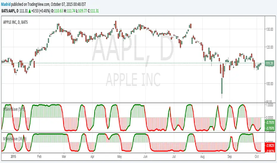
This implements the Even Better Sinewave indicator as described in the book Cycle Analysis for Traders by John F. Ehlers.
In the example I used 36 as the cycle to be analyzed and a second cycle with a shorter period, 9, the larger period tells where the dominant cycle is heading, and the faster cycle signals entry/exit points and reversals.
In the example I used 36 as the cycle to be analyzed and a second cycle with a shorter period, 9, the larger period tells where the dominant cycle is heading, and the faster cycle signals entry/exit points and reversals.
Açık kaynak kodlu komut dosyası
Gerçek TradingView ruhuna uygun olarak, bu komut dosyasının oluşturucusu bunu açık kaynaklı hale getirmiştir, böylece yatırımcılar betiğin işlevselliğini inceleyip doğrulayabilir. Yazara saygı! Ücretsiz olarak kullanabilirsiniz, ancak kodu yeniden yayınlamanın Site Kurallarımıza tabi olduğunu unutmayın.
Feragatname
Bilgiler ve yayınlar, TradingView tarafından sağlanan veya onaylanan finansal, yatırım, işlem veya diğer türden tavsiye veya tavsiyeler anlamına gelmez ve teşkil etmez. Kullanım Şartları'nda daha fazlasını okuyun.