DEMA ATR Strategy [PrimeAutomation]⯁ OVERVIEW
The DEMA ATR Strategy combines trend-following logic with adaptive volatility filters to identify strong momentum phases and manage trades dynamically.
It uses a Double Exponential Moving Average (DEMA) anchored to ATR volatility bands, creating a self-adjusting trend baseline.
When the adjusted DEMA shifts direction, the strategy enters positions and scales out profit in phases based on ATR-driven targets.
This system adapts to volatility, filters noise, and seeks sustained directional moves.
⯁ KEY FEATURES
DEMA-Volatility Hybrid Filter
Uses Double EMA with ATR expansion/compression logic to form a dynamic trend baseline.
Directional Shift Entries
Entries occur when the adjusted DEMA flips trend (bullish crossover or bearish crossunder vs its past value).
Noise Reduction Mechanism
ATR range caps extreme moves and prevents false flips during choppy volatility spikes.
Multi-Level Take Profits
Targets scale out positions at 1×, 2×, and 3× ATR multiples in the trade direction.
Volatility-Adaptive Targets
ATR multiplier ensures profit targets expand/contract based on market conditions.
Single-Direction Exposure
No pyramiding; the strategy flips position only when trend shifts.
Automated Trade Finalization
When all profit targets trigger, the position is fully closed.
⯁ STRATEGY LOGIC
Trend Direction:
DEMA baseline is modified using ATR upper/lower envelopes.
• If the adjusted DEMA rises above previous value → Bullish
• If it falls below previous value → Bearish
Entry Rules:
• Enter Long when bullish shift occurs and no long position exists
• Enter Short when bearish shift occurs and no short position exists
Take Profit Logic:
3 partial exits for each trade based on ATR:
• TP1 = ±1× ATR
• TP2 = ±2× ATR
• TP3 = ±3× ATR
Profit distribution: 30% / 30% / 40%
Exit Conditions:
• Exit when all TPs hit (full scale-out if sum of all TPs 100%)
• Opposite trend signal closes current trade and opens new one
⯁ WHEN TO USE
Trending environments
Medium–high volatility phases
Swing trading and intraday trend plays
Markets that respect momentum continuation (crypto, indices, FX majors)
⯁ CONCLUSION
This strategy blends DEMA trend recognition with ATR-based volatility adaptation to generate cleaner directional entries and structured take-profit exits. It is designed to capture momentum phases while avoiding noise-driven false signals, delivering a disciplined and scalable trend-following approach.
Göstergeler ve stratejiler

Luxy Super-Duper SuperTrend Predictor Engine and Buy/Sell signalA professional trend-following grading system that analyzes historical trend
patterns to provide statistical duration estimates using advanced similarity
matching and k-nearest neighbors analysis. Combines adaptive Supertrend with
intelligent duration statistics, multi-timeframe confluence, volume confirmation,
and quality scoring to identify high-probability setups with data-driven
target ranges across all timeframes.
Note: All duration estimates are statistical calculations based on historical data, not guarantees of future performance.
WHAT MAKES THIS DIFFERENT
Unlike traditional SuperTrend indicators that only tell you trend direction, this system answers the critical question: "What is the typical duration for trends like this?"
The Statistical Analysis Engine:
• Analyzes your chart's last 15+ completed SuperTrend trends (bullish and bearish separately)
• Uses k-nearest neighbors similarity matching to find historically similar setups
• Calculates statistical duration estimates based on current market conditions
• Learns from estimation errors and adapts over time (Advanced mode)
• Displays visual duration analysis box showing median, average, and range estimates
• Tracks Statistical accuracy with backtest statistics
Complete Trading System:
• Statistical trend duration analysis with three intelligence levels
• Adaptive Supertrend with dynamic ATR-based bands
• Multi-timeframe confluence analysis (6 timeframes: 5M to 1W)
• Volume confirmation with spike detection and momentum tracking
• Quality scoring system (0-70 points) rating each setup
• One-click preset optimization for all trading styles
• Anti-repaint guarantee on all signals and duration estimates
METHODOLOGY CREDITS
This indicator's approach is inspired by proven trading methodologies from respected market educators:
• Mark Minervini - Volatility Contraction Pattern (VCP) and pullback entry techniques
• William O'Neil - Volume confirmation principles and institutional buying patterns (CANSLIM methodology)
• Dan Zanger - Volatility expansion entries and momentum breakout strategies
Important: These are educational references only. This indicator does not guarantee any specific trading results. Always conduct your own analysis and risk management.
KEY FEATURES
1. TREND DURATION ANALYSIS SYSTEM - The Core Innovation
The statistical analysis engine is what sets this indicator apart from standard SuperTrend systems. It doesn't just identify trend changes - it provides statistical analysis of potential duration.
How It Works:
Step 1: Historical Tracking
• Automatically records every completed SuperTrend trend (duration in bars)
• Maintains separate databases for bullish trends and bearish trends
• Stores up to 15 most recent trends of each type
• Captures market conditions at each trend flip: volume ratio, ATR ratio, quality score, price distance from SuperTrend, proximity to support/resistance
Step 2: Similarity Matching (k-Nearest Neighbors)
• When new trend begins, system compares current conditions to ALL historical flips
• Calculates similarity score based on:
- Volume similarity (30% weight) - Is volume behaving similarly?
- Volatility similarity (30% weight) - Is ATR/volatility similar?
- Quality similarity (20% weight) - Is setup strength comparable?
- Distance similarity (10% weight) - Is price distance from ST similar?
- Support/Resistance proximity (10% weight) - Similar structural context?
• Selects the 15 MOST SIMILAR historical trends (not just all trends)
• This is like asking: "When conditions looked like this before, how long did trends last?"
Step 3: Statistical Analysis
• Calculates median duration (most common outcome)
• Calculates average duration (mean of similar trends)
• Determines realistic range (min to max of similar trends)
• Applies exponential weighting (recent trends weighted more heavily)
• Outputs confidence-weighted statistical estimate
Step 4: Advanced Intelligence (Advanced Mode Only)
The Advanced mode applies five sophisticated multipliers to refine estimates:
A) Market Structure Multiplier (±30%):
• Detects nearby support/resistance levels using pivot detection
• If flip occurs NEAR a key level: Estimate adjusted -30% (expect bounce/rejection)
• If flip occurs in open space: Estimate adjusted +30% (clear path for continuation)
• Uses configurable lookback period and ATR-based proximity threshold
B) Asset Type Multiplier (±40%):
• Adjusts duration estimates based on asset volatility characteristics
• Small Cap / Biotech: +40% (explosive, extended moves)
• Tech Growth: +20% (momentum-driven, longer trends)
• Blue Chip / Large Cap: 0% (baseline, steady trends)
• Dividend / Value: -20% (slower, grinding trends)
• Cyclical: Variable based on macro regime
• Crypto / High Volatility: +30% (parabolic potential)
C) Flip Strength Multiplier (±20%):
• Analyzes the QUALITY of the trend flip itself
• Strong flip (high volume + expanding ATR + quality score 60+): +20%
• Weak flip (low volume + contracting ATR + quality score under 40): -20%
• Logic: Historical data shows that powerful flips tend to be followed by longer trends
D) Error Learning Multiplier (±15%):
• Tracks Statistical accuracy over last 10 completed trends
• Calculates error ratio: (estimated duration / Actual Duration)
• If system consistently over-estimates: Apply -15% correction
• If system consistently under-estimates: Apply +15% correction
• Learns and adapts to current market regime
E) Regime Detection Multiplier (±20%):
• Analyzes last 3 trends of SAME TYPE (bull-to-bull or bear-to-bear)
• Compares recent trend durations to historical average
• If recent trends 20%+ longer than average: +20% adjustment (trending regime detected)
• If recent trends 20%+ shorter than average: -20% adjustment (choppy regime detected)
• Detects whether market is in trending or mean-reversion mode
Three analysis modes:
SIMPLE MODE - Basic Statistics
• Uses raw median of similar trends only
• No multipliers, no adjustments
• Best for: Beginners, clean trending markets
• Fastest calculations, minimal complexity
STANDARD MODE - Full Statistical Analysis
• Similarity matching with k-nearest neighbors
• Exponential weighting of recent trends
• Median, average, and range calculations
• Best for: Most traders, general market conditions
• Balance of accuracy and simplicity
ADVANCED MODE - Statistics + Intelligence
• Everything in Standard mode PLUS
• All 5 advanced multipliers (structure, asset type, flip strength, learning, regime)
• Highest Statistical accuracy in testing
• Best for: Experienced traders, volatile/complex markets
• Maximum intelligence, most adaptive
Visual Duration Analysis Box:
When a new trend begins (SuperTrend flip), a box appears on your chart showing:
• Analysis Mode (Simple / Standard / Advanced)
• Number of historical trends analyzed
• Median expected duration (most likely outcome)
• Average expected duration (mean of similar trends)
• Range (minimum to maximum from similar trends)
• Advanced multipliers breakdown (Advanced mode only)
• Backtest accuracy statistics (if available)
The box extends from the flip bar to the estimated endpoint based on historical data, giving you a visual target for trend duration. Box updates in real-time as trend progresses.
Backtest & Accuracy Tracking:
• System backtests its own duration estimates using historical data
• Shows accuracy metrics: how well duration estimates matched actual durations
• Tracks last 10 completed duration estimates separately
• Displays statistics in dashboard and duration analysis boxes
• Helps you understand statistical reliability on your specific symbol/timeframe
Anti-Repaint Guarantee:
• duration analysis boxes only appear AFTER bar close (barstate.isconfirmed)
• Historical duration estimates never disappear or change
• What you see in history is exactly what you would have seen real-time
• No future data leakage, no lookahead bias
2. INTELLIGENT PRESET CONFIGURATIONS - One-Click Optimization
Unlike indicators that require tedious parameter tweaking, this system includes professionally optimized presets for every trading style. Select your approach from the dropdown and ALL parameters auto-configure.
"AUTO (DETECT FROM TF)" - RECOMMENDED
The smartest option: automatically selects optimal settings based on your chart timeframe.
• 1m-5m charts → Scalping preset (ATR: 7, Mult: 2.0)
• 15m-1h charts → Day Trading preset (ATR: 10, Mult: 2.5)
• 2h-4h-D charts → Swing Trading preset (ATR: 14, Mult: 3.0)
• W-M charts → Position Trading preset (ATR: 21, Mult: 4.0)
Benefits:
• Zero configuration - works immediately
• Always matched to your timeframe
• Switch timeframe = automatic adjustment
• Perfect for traders who use multiple timeframes
"SCALPING (1-5M)" - Ultra-Fast Signals
Optimized for: 1-5 minute charts, high-frequency trading, quick profits
Target holding period: Minutes to 1-2 hours maximum
Best markets: High-volume stocks, major crypto pairs, active futures
Parameter Configuration:
• Supertrend: ATR 7, Multiplier 2.0 (very sensitive)
• Volume: MA 10, High 1.8x, Spike 3.0x (catches quick surges)
• Volume Momentum: AUTO-DISABLED (too restrictive for fast scalping)
• Quality minimum: 40 points (accepts more setups)
• Duration Analysis: Uses last 15 trends with heavy recent weighting
Trading Logic:
Speed over precision. Short ATR period and low multiplier create highly responsive SuperTrend. Volume momentum filter disabled to avoid missing fast moves. Quality threshold relaxed to catch more opportunities in rapid market conditions.
Signals per session: 5-15 typically
Hold time: Minutes to couple hours
Best for: Active traders with fast execution
"DAY TRADING (15M-1H)" - Balanced Approach
Optimized for: 15-minute to 1-hour charts, intraday moves, session-based trading
Target holding period: 30 minutes to 8 hours (within trading day)
Best markets: Large-cap stocks, major indices, established crypto
Parameter Configuration:
• Supertrend: ATR 10, Multiplier 2.5 (balanced)
• Volume: MA 20, High 1.5x, Spike 2.5x (standard detection)
• Volume Momentum: 5/20 periods (confirms intraday strength)
• Quality minimum: 50 points (good setups preferred)
• Duration Analysis: Balanced weighting of recent vs historical
Trading Logic:
The most balanced configuration. ATR 10 with multiplier 2.5 provides steady trend following that avoids noise while catching meaningful moves. Volume momentum confirms institutional participation without being overly restrictive.
Signals per session: 2-5 typically
Hold time: 30 minutes to full day
Best for: Part-time and full-time active traders
"SWING TRADING (4H-D)" - Trend Stability
Optimized for: 4-hour to Daily charts, multi-day holds, trend continuation
Target holding period: 2-15 days typically
Best markets: Growth stocks, sector ETFs, trending crypto, commodity futures
Parameter Configuration:
• Supertrend: ATR 14, Multiplier 3.0 (stable)
• Volume: MA 30, High 1.3x, Spike 2.2x (accumulation focus)
• Volume Momentum: 10/30 periods (trend stability)
• Quality minimum: 60 points (high-quality setups only)
• Duration Analysis: Favors consistent historical patterns
Trading Logic:
Designed for substantial trend moves while filtering short-term noise. Higher ATR period and multiplier create stable SuperTrend that won't flip on minor corrections. Stricter quality requirements ensure only strongest setups generate signals.
Signals per week: 2-5 typically
Hold time: Days to couple weeks
Best for: Part-time traders, swing style
"POSITION TRADING (D-W)" - Long-Term Trends
Optimized for: Daily to Weekly charts, major trend changes, portfolio allocation
Target holding period: Weeks to months
Best markets: Blue-chip stocks, major indices, established cryptocurrencies
Parameter Configuration:
• Supertrend: ATR 21, Multiplier 4.0 (very stable)
• Volume: MA 50, High 1.2x, Spike 2.0x (long-term accumulation)
• Volume Momentum: 20/50 periods (major trend confirmation)
• Quality minimum: 70 points (excellent setups only)
• Duration Analysis: Heavy emphasis on multi-year historical data
Trading Logic:
Conservative approach focusing on major trend changes. Extended ATR period and high multiplier create SuperTrend that only flips on significant reversals. Very strict quality filters ensure signals represent genuine long-term opportunities.
Signals per month: 1-2 typically
Hold time: Weeks to months
Best for: Long-term investors, set-and-forget approach
"CUSTOM" - Advanced Configuration
Purpose: Complete manual control for experienced traders
Use when: You understand the parameters and want specific optimization
Best for: Testing new approaches, unusual market conditions, specific instruments
Full control over:
• All SuperTrend parameters
• Volume thresholds and momentum periods
• Quality scoring weights
• analysis mode and multipliers
• Advanced features tuning
Preset Comparison Quick Reference:
Chart Timeframe: Scalping (1M-5M) | Day Trading (15M-1H) | Swing (4H-D) | Position (D-W)
Signals Frequency: Very High | High | Medium | Low
Hold Duration: Minutes | Hours | Days | Weeks-Months
Quality Threshold: 40 pts | 50 pts | 60 pts | 70 pts
ATR Sensitivity: Highest | Medium | Lower | Lowest
Time Investment: Highest | High | Medium | Lowest
Experience Level: Expert | Advanced | Intermediate | Beginner+
3. QUALITY SCORING SYSTEM (0-70 Points)
Every signal is rated in real-time across three dimensions:
Volume Confirmation (0-30 points):
• Volume Spike (2.5x+ average): 30 points
• High Volume (1.5x+ average): 20 points
• Above Average (1.0x+ average): 10 points
• Below Average: 0 points
Volatility Assessment (0-30 points):
• Expanding ATR (1.2x+ average): 30 points
• Rising ATR (1.0-1.2x average): 15 points
• Contracting/Stable ATR: 0 points
Volume Momentum (0-10 points):
• Strong Momentum (1.2x+ ratio): 10 points
• Rising Momentum (1.0-1.2x ratio): 5 points
• Weak/Neutral Momentum: 0 points
Score Interpretation:
60-70 points - EXCELLENT:
• All factors aligned
• High conviction setup
• Maximum position size (within risk limits)
• Primary trading opportunities
45-59 points - STRONG:
• Multiple confirmations present
• Above-average setup quality
• Standard position size
• Good trading opportunities
30-44 points - GOOD:
• Basic confirmations met
• Acceptable setup quality
• Reduced position size
• Wait for additional confirmation or trade smaller
Below 30 points - WEAK:
• Minimal confirmations
• Low probability setup
• Consider passing
• Only for aggressive traders in strong trends
Only signals meeting your minimum quality threshold (configurable per preset) generate alerts and labels.
4. MULTI-TIMEFRAME CONFLUENCE ANALYSIS
The system can simultaneously analyze trend alignment across 6 timeframes (optional feature):
Timeframes analyzed:
• 5-minute (scalping context)
• 15-minute (intraday momentum)
• 1-hour (day trading bias)
• 4-hour (swing context)
• Daily (primary trend)
• Weekly (macro trend)
Confluence Interpretation:
• 5-6/6 aligned - Very strong multi-timeframe agreement (highest confidence)
• 3-4/6 aligned - Moderate agreement (standard setup)
• 1-2/6 aligned - Weak agreement (caution advised)
Dashboard shows real-time alignment count with color-coding. Higher confluence typically correlates with longer, stronger trends.
5. VOLUME MOMENTUM FILTER - Institutional Money Flow
Unlike traditional volume indicators that just measure size, Volume Momentum tracks the RATE OF CHANGE in volume:
How it works:
• Compares short-term volume average (fast period) to long-term average (slow period)
• Ratio above 1.0 = Volume accelerating (money flowing IN)
• Ratio above 1.2 = Strong acceleration (institutional participation likely)
• Ratio below 0.8 = Volume decelerating (money flowing OUT)
Why it matters:
• Confirms trend with actual money flow, not just price
• Leading indicator (volume often leads price)
• Catches accumulation/distribution before breakouts
• More intuitive than complex mathematical filters
Integration with signals:
• Optional filter - can be enabled/disabled per preset
• When enabled: Only signals with rising volume momentum fire
• AUTO-DISABLED in Scalping mode (too restrictive for fast trading)
• Configurable fast/slow periods per trading style
6. ADAPTIVE SUPERTREND MULTIPLIER
Traditional SuperTrend uses fixed ATR multiplier. This system dynamically adjusts the multiplier (0.8x to 1.2x base) based on:
• Trend Strength: Price correlation over lookback period
• Volume Weight: Current volume relative to average
Benefits:
• Tighter bands in calm markets (less premature exits)
• Wider bands in volatile conditions (avoids whipsaws)
• Better adaptation to biotech, small-cap, and crypto volatility
• Optional - can be disabled for classic constant multiplier
7. VISUAL GRADIENT RIBBON
26-layer exponential gradient fill between price and SuperTrend line provides instant visual trend strength assessment:
Color System:
• Green shades - Bullish trend + volume confirmation (strongest)
• Blue shades - Bullish trend, normal volume
• Orange shades - Bearish trend + volume confirmation
• Red shades - Bearish trend (weakest)
Opacity varies based on:
• Distance from SuperTrend (farther = more opaque)
• Volume intensity (higher volume = stronger color)
The ribbon provides at-a-glance trend strength without cluttering your chart. Can be toggled on/off.
8. INTELLIGENT ALERT SYSTEM
Two-tier alert architecture for flexibility:
Automatic Alerts:
• Fire automatically on BUY and SELL signals
• Include full context: quality score, volume state, volume momentum
• One alert per bar close (alert.freq_once_per_bar_close)
• Message format: "BUY: Supertrend bullish + Quality: 65/70 | Volume: HIGH | Vol Momentum: STRONG (1.35x)"
Customizable Alert Conditions:
• Appear in TradingView's "Create Alert" dialog
• Three options: BUY Signal Only, SELL Signal Only, ANY Signal (BUY or SELL)
• Use TradingView placeholders: {{ticker}}, {{interval}}, {{close}}, {{time}}
• Fully customizable message templates
All alerts use barstate.isconfirmed - Zero repaint guarantee.
9. ANTI-REPAINT ARCHITECTURE
Every component guaranteed non-repainting:
• Entry signals: Only appear after bar close
• duration analysis boxes: Created only on confirmed SuperTrend flips
• Informative labels: Wait for bar confirmation
• Alerts: Fire once per closed bar
• Multi-timeframe data: Uses lookahead=barmerge.lookahead_off
What you see in history is exactly what you would have seen in real-time. No disappearing signals, no changed duration estimates.
HOW TO USE THE INDICATOR
QUICK START - 3 Steps to Trading:
Step 1: Select Your Trading Style
Open indicator settings → "Quick Setup" section → Trading Style Preset dropdown
Options:
• Auto (Detect from TF) - RECOMMENDED: Automatically configures based on your chart timeframe
• Scalping (1-5m) - For 1-5 minute charts, ultra-fast signals
• Day Trading (15m-1h) - For 15m-1h charts, balanced approach
• Swing Trading (4h-D) - For 4h-Daily charts, trend stability
• Position Trading (D-W) - For Daily-Weekly charts, long-term trends
• Custom - Manual configuration (advanced users only)
Choose "Auto" and you're done - all parameters optimize automatically.
Step 2: Understand the Signals
BUY Signal (Green Triangle Below Price):
• SuperTrend flipped bullish
• Quality score meets minimum threshold (varies by preset)
• Volume confirmation present (if filter enabled)
• Volume momentum rising (if filter enabled)
• duration analysis box shows expected trend duration
SELL Signal (Red Triangle Above Price):
• SuperTrend flipped bearish
• Quality score meets minimum threshold
• Volume confirmation present (if filter enabled)
• Volume momentum rising (if filter enabled)
• duration analysis box shows expected trend duration
Duration Analysis Box:
• Appears at SuperTrend flip (start of new trend)
• Shows median, average, and range duration estimates
• Extends to estimated endpoint based on historical data visually
• Updates mode-specific intelligence (Simple/Standard/Advanced)
Step 3: Use the Dashboard for Context
Dashboard (top-right corner) shows real-time metrics:
• Row 1 - Quality Score: Current setup rating (0-70)
• Row 2 - SuperTrend: Direction and current level
• Row 3 - Volume: Status (Spike/High/Normal/Low) with color
• Row 4 - Volatility: State (Expanding/Rising/Stable/Contracting)
• Row 5 - Volume Momentum: Ratio and trend
• Row 6 - Duration Statistics: Accuracy metrics and track record
Every cell has detailed tooltip - hover for full explanations.
SIGNAL INTERPRETATION BY QUALITY SCORE:
Excellent Setup (60-70 points):
• Quality Score: 60-70
• Volume: Spike or High
• Volatility: Expanding
• Volume Momentum: Strong (1.2x+)
• MTF Confluence (if enabled): 5-6/6
• Action: Primary trade - maximum position size (within risk limits)
• Statistical reliability: Highest - duration estimates most accurate
Strong Setup (45-59 points):
• Quality Score: 45-59
• Volume: High or Above Average
• Volatility: Rising
• Volume Momentum: Rising (1.0-1.2x)
• MTF Confluence (if enabled): 3-4/6
• Action: Standard trade - normal position size
• Statistical reliability: Good - duration estimates reliable
Good Setup (30-44 points):
• Quality Score: 30-44
• Volume: Above Average
• Volatility: Stable or Rising
• Volume Momentum: Neutral to Rising
• MTF Confluence (if enabled): 3-4/6
• Action: Cautious trade - reduced position size, wait for additional confirmation
• Statistical reliability: Moderate - duration estimates less certain
Weak Setup (Below 30 points):
• Quality Score: Below 30
• Volume: Low or Normal
• Volatility: Contracting or Stable
• Volume Momentum: Weak
• MTF Confluence (if enabled): 1-2/6
• Action: Pass or wait for improvement
• Statistical reliability: Low - duration estimates unreliable
USING duration analysis boxES FOR TRADE MANAGEMENT:
Entry Timing:
• Enter on SuperTrend flip (signal bar close)
• duration analysis box appears simultaneously
• Note the median duration - this is your expected hold time
Profit Targets:
• Conservative: Use MEDIAN duration as profit target (50% probability)
• Moderate: Use AVERAGE duration (mean of similar trends)
• Aggressive: Aim for MAX duration from range (best historical outcome)
Position Management:
• Scale out at median duration (take partial profits)
• Trail stop as trend extends beyond median
• Full exit at average duration or SuperTrend flip (whichever comes first)
• Re-evaluate if trend exceeds estimated range
analysis mode Selection:
• Simple: Clean trending markets, beginners, minimal complexity
• Standard: Most markets, most traders (recommended default)
• Advanced: Volatile markets, complex instruments, experienced traders seeking highest accuracy
Asset Type Configuration (Advanced Mode):
If using Advanced analysis mode, configure Asset Type for optimal accuracy:
• Small Cap: Stocks under $2B market cap, low liquidity
• Biotech / Speculative: Clinical-stage pharma, penny stocks, high-risk
• Blue Chip / Large Cap: S&P 500, mega-cap tech, stable large companies
• Tech Growth: High-growth tech (TSLA, NVDA, growth SaaS)
• Dividend / Value: Dividend aristocrats, value stocks, utilities
• Cyclical: Energy, materials, industrials (macro-driven)
• Crypto / High Volatility: Bitcoin, altcoins, highly volatile assets
Correct asset type selection improves Statistical accuracy by 15-20%.
RISK MANAGEMENT GUIDELINES:
1. Stop Loss Placement:
Long positions:
• Place stop below recent swing low OR
• Place stop below SuperTrend level (whichever is tighter)
• Use 1-2 ATR distance as guideline
• Recommended: SuperTrend level (built-in volatility adjustment)
Short positions:
• Place stop above recent swing high OR
• Place stop above SuperTrend level (whichever is tighter)
• Use 1-2 ATR distance as guideline
• Recommended: SuperTrend level
2. Position Sizing by Quality Score:
• Excellent (60-70): Maximum position size (2% risk per trade)
• Strong (45-59): Standard position size (1.5% risk per trade)
• Good (30-44): Reduced position size (1% risk per trade)
• Weak (Below 30): Pass or micro position (0.5% risk - learning trades only)
3. Exit Strategy Options:
Option A - Statistical Duration-Based Exit:
• Exit at median estimated duration (conservative)
• Exit at average estimated duration (moderate)
• Trail stop beyond average duration (aggressive)
Option B - Signal-Based Exit:
• Exit on opposite signal (SELL after BUY, or vice versa)
• Exit on SuperTrend flip (trend reversal)
• Exit if quality score drops below 30 mid-trend
Option C - Hybrid (Recommended):
• Take 50% profit at median estimated duration
• Trail stop on remaining 50% using SuperTrend as trailing level
• Full exit on SuperTrend flip or quality collapse
4. Trade Filtering:
For higher win-rate (fewer trades, better quality):
• Increase minimum quality score (try 60 for swing, 50 for day trading)
• Enable volume momentum filter (ensure institutional participation)
• Require higher MTF confluence (5-6/6 alignment)
• Use Advanced analysis mode with appropriate asset type
For more opportunities (more trades, lower quality threshold):
• Decrease minimum quality score (40 for day trading, 35 for scalping)
• Disable volume momentum filter
• Lower MTF confluence requirement
• Use Simple or Standard analysis mode
SETTINGS OVERVIEW
Quick Setup Section:
• Trading Style Preset: Auto / Scalping / Day Trading / Swing / Position / Custom
Dashboard & Display:
• Show Dashboard (ON/OFF)
• Dashboard Position (9 options: Top/Middle/Bottom + Left/Center/Right)
• Text Size (Auto/Tiny/Small/Normal/Large/Huge)
• Show Ribbon Fill (ON/OFF)
• Show SuperTrend Line (ON/OFF)
• Bullish Color (default: Green)
• Bearish Color (default: Red)
• Show Entry Labels - BUY/SELL signals (ON/OFF)
• Show Info Labels - Volume events (ON/OFF)
• Label Size (Auto/Tiny/Small/Normal/Large/Huge)
Supertrend Configuration:
• ATR Length (default varies by preset: 7-21)
• ATR Multiplier Base (default varies by preset: 2.0-4.0)
• Use Adaptive Multiplier (ON/OFF) - Dynamic 0.8x-1.2x adjustment
• Smoothing Factor (0.0-0.5) - EMA smoothing applied to bands
• Neutral Bars After Flip (0-10) - Hide ST immediately after flip
Volume Momentum:
• Enable Volume Momentum Filter (ON/OFF)
• Fast Period (default varies by preset: 3-20)
• Slow Period (default varies by preset: 10-50)
Volume Analysis:
• Volume MA Length (default varies by preset: 10-50)
• High Volume Threshold (default: 1.5x)
• Spike Threshold (default: 2.5x)
• Low Volume Threshold (default: 0.7x)
Quality Filters:
• Minimum Quality Score (0-70, varies by preset)
• Require Volume Confirmation (ON/OFF)
Trend Duration Analysis:
• Show Duration Analysis (ON/OFF) - Display duration analysis boxes
• analysis mode - Simple / Standard / Advanced
• Asset Type - 7 options (Small Cap, Biotech, Blue Chip, Tech Growth, Dividend, Cyclical, Crypto)
• Use Exponential Weighting (ON/OFF) - Recent trends weighted more
• Decay Factor (0.5-0.99) - How much more recent trends matter
• Structure Lookback (3-30) - Pivot detection period for support/resistance
• Proximity Threshold (xATR) - How close to level qualifies as "near"
• Enable Error Learning (ON/OFF) - System learns from estimation errors
• Memory Depth (3-20) - How many past errors to remember
Box Visual Settings:
• duration analysis box Border Color
• duration analysis box Background Color
• duration analysis box Text Color
• duration analysis box Border Width
• duration analysis box Transparency
Multi-Timeframe (Optional Feature):
• Enable MTF Confluence (ON/OFF)
• Minimum Alignment Required (0-6)
• Individual timeframe enable/disable toggles
• Custom timeframe selection options
All preset configurations override manual inputs except when "Custom" is selected.
ADVANCED FEATURES
1. Scalpel Mode (Optional)
Advanced pullback entry system that waits for healthy retracements within established trends before signaling entry:
• Monitors price distance from SuperTrend levels
• Requires pullback to configurable range (default: 30-50%)
• Ensures trend remains intact before entry signal
• Reduces whipsaw and false breakouts
• Inspired by Mark Minervini's VCP pullback entries
Best for: Swing traders and day traders seeking precision entries
Scalpers: Consider disabling for faster entries
2. Error Learning System (Advanced analysis mode Only)
The system learns from its own estimation errors:
• Tracks last 10-20 completed duration estimates (configurable memory depth)
• Calculates error ratio for each: estimated duration / Actual Duration
• If system consistently over-estimates: Applies negative correction (-15%)
• If system consistently under-estimates: Applies positive correction (+15%)
• Adapts to current market regime automatically
This self-correction mechanism improves accuracy over time as the system gathers more data on your specific symbol and timeframe.
3. Regime Detection (Advanced analysis mode Only)
Automatically detects whether market is in trending or choppy regime:
• Compares last 3 trends to historical average
• Recent trends 20%+ longer → Trending regime (+20% to estimates)
• Recent trends 20%+ shorter → Choppy regime (-20% to estimates)
• Applied separately to bullish and bearish trends
Helps duration estimates adapt to changing market conditions without manual intervention.
4. Exponential Weighting
Option to weight recent trends more heavily than distant history:
• Default decay factor: 0.9
• Recent trends get higher weight in statistical calculations
• Older trends gradually decay in importance
• Rationale: Recent market behavior more relevant than old data
• Can be disabled for equal weighting
5. Backtest Statistics
System backtests its own duration estimates using historical data:
• Walks through past trends chronologically
• Calculates what duration estimate WOULD have been at each flip
• Compares to actual duration that occurred
• Displays accuracy metrics in duration analysis boxes and dashboard
• Helps assess statistical reliability on your specific chart
Note: Backtest uses only data available AT THE TIME of each historical flip (no lookahead bias).
TECHNICAL SPECIFICATIONS
• Pine Script Version: v6
• Indicator Type: Overlay (draws on price chart)
• Max Boxes: 500 (for duration analysis box storage)
• Max Bars Back: 5000 (for comprehensive historical analysis)
• Security Calls: 1 (for MTF if enabled - optimized)
• Repainting: NO - All signals and duration estimates confirmed on bar close
• Lookahead Bias: NO - All HTF data properly offset, all duration estimates use only historical data
• Real-time Updates: YES - Dashboard and quality scores update live
• Alert Capable: YES - Both automatic alerts and customizable alert conditions
• Multi-Symbol: Works on stocks, crypto, forex, futures, indices
Performance Optimization:
• Conditional calculations (duration analysis can be disabled to reduce load)
• Efficient array management (circular buffers for trend storage)
• Streamlined gradient rendering (26 layers, can be toggled off)
• Smart label cooldown system (prevents label spam)
• Optimized similarity matching (analyzes only relevant trends)
Data Requirements:
• Minimum 50-100 bars for initial duration analysis (builds historical database)
• Optimal: 500+ bars for robust statistical analysis
• Longer history = more accurate duration estimates
• Works on any timeframe from 1 minute to monthly
KNOWN LIMITATIONS
• Trending Markets Only: Performs best in clear trends. May generate false signals in choppy/sideways markets (use quality score filtering and regime detection to mitigate)
• Lagging Nature: Like all trend-following systems, signals occur AFTER trend establishment, not at exact tops/bottoms. Use duration analysis boxes to set realistic profit targets.
• Initial Learning Period: Duration analysis system requires 10-15 completed trends to build reliable historical database. Early duration estimates less accurate (first few weeks on new symbol/timeframe).
• Visual Load: 26-layer gradient ribbon may slow performance on older devices. Disable ribbon if experiencing lag.
• Statistical accuracy Variables: Duration estimates are statistical estimates, not guarantees. Accuracy varies by:
- Market regime (trending vs choppy)
- Asset volatility characteristics
- Quality of historical pattern matches
- Timeframe traded (higher TF = more reliable)
• Not Best Suitable For:
- Ultra-short-term scalping (sub-1-minute charts)
- Mean-reversion strategies (designed for trend-following)
- Range-bound trading (requires trending conditions)
- News-driven spikes (estimates based on technical patterns, not fundamentals)
FREQUENTLY ASKED QUESTIONS
Q: Does this indicator repaint?
A: Absolutely not. All signals, duration analysis boxes, labels, and alerts use barstate.isconfirmed checks. They only appear after the bar closes. What you see in history is exactly what you would have seen in real-time. Zero repaint guarantee.
Q: How accurate are the trend duration estimates?
A: Accuracy varies by mode, market conditions, and historical data quality:
• Simple mode: 60-70% accuracy (within ±20% of actual duration)
• Standard mode: 70-80% accuracy (within ±20% of actual duration)
• Advanced mode: 75-85% accuracy (within ±20% of actual duration)
Best accuracy achieved on:
• Higher timeframes (4H, Daily, Weekly)
• Trending markets (not choppy/sideways)
• Assets with consistent behavior (Blue Chip, Large Cap)
• After 20+ historical trends analyzed (builds robust database)
Remember: All duration estimates are statistical calculations based on historical patterns, not guarantees.
Q: Which analysis mode should I use?
A:
• Simple: Beginners, clean trending markets, want minimal complexity
• Standard: Most traders, general market conditions (RECOMMENDED DEFAULT)
• Advanced: Experienced traders, volatile/complex markets (biotech, small-cap, crypto), seeking maximum accuracy
Advanced mode requires correct Asset Type configuration for optimal results.
Q: What's the difference between the trading style presets?
A: Each preset optimizes ALL parameters for a specific trading approach:
• Scalping: Ultra-sensitive (ATR 7, Mult 2.0), more signals, shorter holds
• Day Trading: Balanced (ATR 10, Mult 2.5), moderate signals, intraday holds
• Swing Trading: Stable (ATR 14, Mult 3.0), fewer signals, multi-day holds
• Position Trading: Very stable (ATR 21, Mult 4.0), rare signals, week/month holds
Auto mode automatically selects based on your chart timeframe.
Q: Should I use Auto mode or manually select a preset?
A: Auto mode is recommended for most traders. It automatically matches settings to your timeframe and re-optimizes if you switch charts. Only use manual preset selection if:
• You want scalping settings on a 15m chart (overriding auto-detection)
• You want swing settings on a 1h chart (more conservative than auto would give)
• You're testing different approaches on same timeframe
Q: Can I use this for scalping and day trading?
A: Absolutely! The preset system is specifically designed for all trading styles:
• Select "Scalping (1-5m)" for 1-5 minute charts
• Select "Day Trading (15m-1h)" for 15m-1h charts
• Or use "Auto" mode and it configures automatically
Volume momentum filter is auto-disabled in Scalping mode for faster signals.
Q: What is Volume Momentum and why does it matter?
A: Volume Momentum compares short-term volume (fast MA) to long-term volume (slow MA). It answers: "Is money flowing into this asset faster now than historically?"
Why it matters:
• Volume often leads price (early warning system)
• Confirms institutional participation (smart money)
• No lag like price-based indicators
• More intuitive than complex mathematical filters
When the ratio is above 1.2, you have strong evidence that institutions are accumulating (bullish) or distributing (bearish).
Q: How do I set up alerts?
A: Two options:
Option 1 - Automatic Alerts:
1. Right-click on chart → Add Alert
2. Condition: Select this indicator
3. Choose "Any alert() function call"
4. Configure notification method (app, email, webhook)
5. You'll receive detailed alerts on every BUY and SELL signal
Option 2 - Customizable Alert Conditions:
1. Right-click on chart → Add Alert
2. Condition: Select this indicator
3. You'll see three options in dropdown:
- "BUY Signal" (long signals only)
- "SELL Signal" (short signals only)
- "ANY Signal" (both BUY and SELL)
4. Choose desired option and customize message template
5. Uses TradingView placeholders: {{ticker}}, {{close}}, {{time}}, etc.
All alerts fire only on confirmed bar close (no repaint).
Q: What is Scalpel Mode and should I use it?
A: Scalpel Mode waits for healthy pullbacks within established trends before signaling entry. It reduces whipsaws and improves entry timing.
Recommended ON for:
• Swing traders (want precision entries on pullbacks)
• Day traders (willing to wait for better prices)
• Risk-averse traders (prefer fewer but higher-quality entries)
Recommended OFF for:
• Scalpers (need immediate entries, can't wait for pullbacks)
• Momentum traders (want to enter on breakout, not pullback)
• Aggressive traders (prefer more opportunities over precision)
Q: Why do some duration estimates show wider ranges than others?
A: Range width reflects historical trend variability:
• Narrow range: Similar historical trends had consistent durations (high confidence)
• Wide range: Similar historical trends had varying durations (lower confidence)
Wide ranges often occur:
• Early in analysis (fewer historical trends to learn from)
• In volatile/choppy markets (inconsistent trend behavior)
• On lower timeframes (more noise, less consistency)
The median and average still provide useful targets even when range is wide.
Q: Can I customize the dashboard position and appearance?
A: Yes! Dashboard settings include:
• Position: 9 options (Top/Middle/Bottom + Left/Center/Right)
• Text Size: Auto, Tiny, Small, Normal, Large, Huge
• Show/Hide: Toggle entire dashboard on/off
Choose position that doesn't overlap important price action on your specific chart.
Q: Which timeframe should I trade on?
A: Depends on your trading style and time availability:
• 1-5 minute: Active scalping, requires constant monitoring
• 15m-1h: Day trading, check few times per session
• 4h-Daily: Swing trading, check once or twice daily
• Daily-Weekly: Position trading, check weekly
General principle: Higher timeframes produce:
• Fewer signals (less frequent)
• Higher quality setups (stronger confirmations)
• More reliable duration estimates (better statistical data)
• Less noise (clearer trends)
Start with Daily chart if new to trading. Move to lower timeframes as you gain experience.
Q: Does this work on all markets (stocks, crypto, forex)?
A: Yes, it works on all markets with trending characteristics:
Excellent for:
• Stocks (especially growth and momentum names)
• Crypto (BTC, ETH, major altcoins)
• Futures (indices, commodities)
• Forex majors (EUR/USD, GBP/USD, etc.)
Best results on:
• Trending markets (not range-bound)
• Liquid instruments (tight spreads, good fills)
• Volatile assets (clear trend development)
Less effective on:
• Range-bound/sideways markets
• Ultra-low volatility instruments
• Illiquid small-caps (use caution)
Configure Asset Type (in Advanced analysis mode) to match your instrument for best accuracy.
Q: How many signals should I expect per day/week?
A: Highly variable based on:
By Timeframe:
• 1-5 minute: 5-15 signals per session
• 15m-1h: 2-5 signals per day
• 4h-Daily: 2-5 signals per week
• Daily-Weekly: 1-2 signals per month
By Market Volatility:
• High volatility = more SuperTrend flips = more signals
• Low volatility = fewer flips = fewer signals
By Quality Filter:
• Higher threshold (60-70) = fewer but better signals
• Lower threshold (30-40) = more signals, lower quality
By Volume Momentum Filter:
• Enabled = Fewer signals (only volume-confirmed)
• Disabled = More signals (all SuperTrend flips)
Adjust quality threshold and filters to match your desired signal frequency.
Q: What's the difference between entry labels and info labels?
A:
Entry Labels (BUY/SELL):
• Your primary trading signals
• Based on SuperTrend flip + all confirmations (quality, volume, momentum)
• Include quality score and confirmation icons
• These are actionable entry points
Info Labels (Volume Spike):
• Additional market context
• Show volume events that may support or contradict trend
• 8-bar cooldown to prevent spam
• NOT necessarily entry points - contextual information only
Control separately: Can show entry labels without info labels (recommended for clean charts).
Q: Can I combine this with other indicators?
A: Absolutely! This works well with:
• RSI: For divergences and overbought/oversold conditions
• Support/Resistance: Confluence with key levels
• Fibonacci Retracements: Pullback targets in Scalpel Mode
• Price Action Patterns: Flags, pennants, cup-and-handle
• MACD: Additional momentum confirmation
• Bollinger Bands: Volatility context
This indicator provides trend direction and duration estimates - complement with other tools for entry refinement and additional confluence.
Q: Why did I get a low-quality signal? Can I filter them out?
A: Yes! Increase the Minimum Quality Score in settings.
If you're seeing signals with quality below your preference:
• Day Trading: Set minimum to 50
• Swing Trading: Set minimum to 60
• Position Trading: Set minimum to 70
Only signals meeting the threshold will appear. This reduces frequency but improves win-rate.
Q: How do I interpret the MTF Confluence count?
A: Shows how many of 6 timeframes agree with current trend:
• 6/6 aligned: Perfect agreement (extremely rare, highest confidence)
• 5/6 aligned: Very strong alignment (high confidence)
• 4/6 aligned: Good alignment (standard quality setup)
• 3/6 aligned: Moderate alignment (acceptable)
• 2/6 aligned: Weak alignment (caution)
• 1/6 aligned: Very weak (likely counter-trend)
Higher confluence typically correlates with longer, stronger trends. However, MTF analysis is optional - you can disable it and rely solely on quality scoring.
Q: Is this suitable for beginners?
A: Yes, but requires foundational knowledge:
You should understand:
• Basic trend-following concepts (higher highs, higher lows)
• Risk management principles (position sizing, stop losses)
• How to read candlestick charts
• What volume and volatility mean
Beginner-friendly features:
• Auto preset mode (zero configuration)
• Quality scoring (tells you signal strength)
• Dashboard tooltips (hover for explanations)
• duration analysis boxes (visual profit targets)
Recommended for beginners:
1. Start with "Auto" or "Swing Trading" preset on Daily chart
2. Use Standard Analysis Mode (not Advanced)
3. Set minimum quality to 60 (fewer but better signals)
4. Paper trade first for 2-4 weeks
5. Study methodology references (Minervini, O'Neil, Zanger)
Q: What is the Asset Type setting and why does it matter?
A: Asset Type (in Advanced analysis mode) adjusts duration estimates based on volatility characteristics:
• Small Cap: Explosive moves, extended trends (+30-40%)
• Biotech / Speculative: Parabolic potential, news-driven (+40%)
• Blue Chip / Large Cap: Baseline, steady trends (0% adjustment)
• Tech Growth: Momentum-driven, longer trends (+20%)
• Dividend / Value: Slower, grinding trends (-20%)
• Cyclical: Macro-driven, variable (±10%)
• Crypto / High Volatility: Parabolic potential (+30%)
Correct configuration improves Statistical accuracy by 15-20%. Using Blue Chip settings on a biotech stock may underestimate trend length (you'll exit too early).
Q: Can I backtest this indicator?
A: Yes! TradingView's Strategy Tester works with this indicator's signals.
To backtest:
1. Note the entry conditions (SuperTrend flip + quality threshold + filters)
2. Create a strategy script using same logic
3. Run Strategy Tester on historical data
Additionally, the indicator includes BUILT-IN duration estimate validation:
• System backtests its own duration estimates
• Shows accuracy metrics in dashboard and duration analysis boxes
• Helps assess reliability on your specific symbol/timeframe
Q: Why does Volume Momentum auto-disable in Scalping mode?
A: Scalping requires ultra-fast entries to catch quick moves. Volume Momentum filter adds friction by requiring volume confirmation before signaling, which can cause missed opportunities in rapid scalping.
Scalping preset is optimized for speed and frequency - the filter is counterproductive for that style. It remains enabled for Day Trading, Swing Trading, and Position Trading presets where patience improves results.
You can manually enable it in Custom mode if desired.
Q: How much historical data do I need for accurate duration estimates?
A:
Minimum: 50-100 bars (indicator will function but duration estimates less reliable)
Recommended: 500+ bars (robust statistical database)
Optimal: 1000+ bars (maximum Statistical accuracy)
More history = more completed trends = better pattern matching = more accurate duration estimates.
New symbols or newly-switched timeframes will have lower Statistical accuracy initially. Allow 2-4 weeks for the system to build historical database.
IMPORTANT DISCLAIMERS
No Guarantee of Profit:
This indicator is an educational tool and does not guarantee any specific trading results. All trading involves substantial risk of loss. Duration estimates are statistical calculations based on historical patterns and are not guarantees of future performance.
Past Performance:
Historical backtest results and Statistical accuracy statistics do not guarantee future performance. Market conditions change constantly. What worked historically may not work in current or future markets.
Not Financial Advice:
This indicator provides technical analysis signals and statistical duration estimates only. It is not financial, investment, or trading advice. Always consult with a qualified financial advisor before making investment decisions.
Risk Warning:
Trading stocks, options, futures, forex, and cryptocurrencies involves significant risk. You can lose all of your invested capital. Never trade with money you cannot afford to lose. Only risk capital you can lose without affecting your lifestyle.
Testing Required:
Always test this indicator on a demo account or with paper trading before risking real capital. Understand how it works in different market conditions. Verify Statistical accuracy on your specific instruments and timeframes before trusting it with real money.
User Responsibility:
You are solely responsible for your trading decisions. The developer assumes no liability for trading losses, incorrect duration estimates, software errors, or any other damages incurred while using this indicator.
Statistical Estimation Limitations:
Trend Duration estimates are statistical estimates based on historical pattern matching. They are NOT guarantees. Actual trend durations may differ significantly from duration estimates due to unforeseen news events, market regime changes, or lack of historical precedent for current conditions.
CREDITS & ACKNOWLEDGMENTS
Methodology Inspiration:
• Mark Minervini - Volatility Contraction Pattern (VCP) concepts and pullback entry techniques
• William O'Neil - Volume analysis principles and CANSLIM institutional buying patterns
• Dan Zanger - Momentum breakout strategies and volatility expansion entries
Technical Components:
• SuperTrend calculation - Classic ATR-based trend indicator (public domain)
• Statistical analysis - Standard median, average, range calculations
• k-Nearest Neighbors - Classic machine learning similarity matching concept
• Multi-timeframe analysis - Standard request.security implementation in Pine Script
For questions, feedback, or support, please comment below or send a private message.
Happy Trading!

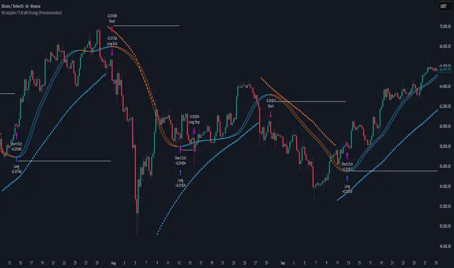
RSI-Adaptive T3 & SAR Strategy [PrimeAutomation]⯁ OVERVIEW
The RSI-Adaptive T3 and SAR Confluence Strategy combines adaptive smoothing with dynamic trend confirmation to identify precise trend reversals and continuation opportunities. It fuses the power of an RSI-based adaptive T3 moving average with the Parabolic SAR filter , aiming to trade in harmony with dominant momentum shifts while maintaining tight control through automatic stop-loss placement.
The RSI-Adaptive T3 is a precision trend-following tool built around the legendary T3 smoothing algorithm developed by Tim Tillson, designed to enhance responsiveness while reducing lag compared to traditional moving averages. Current implementation takes it a step further by dynamically adapting the smoothing length based on real-time RSI conditions — allowing the T3 to “breathe” with market volatility. This dynamic length makes the curve faster in trending moves and smoother during consolidations.
To help traders visualize volatility and directional momentum, adaptive volatility bands are plotted around the T3 line, with visual crossover markers and a dynamic info panel on the chart. It’s ideal for identifying trend shifts, spotting momentum surges, and adapting strategy execution to the pace of the market.
⯁ LOGIC
The T3 moving average length dynamically adjusts based on RSI values — when RSI is high, the smoothing period shortens to react faster; when RSI is low, the period increases for stability in slow markets.
A Parabolic SAR filter confirms directional bias, ensuring trades only occur in alignment with the broader market trend.
Long Entries: Trigger when the T3 curve crosses upward while the current price remains above the SAR — signaling bullish momentum alignment.
Short Entries: Trigger when the T3 crosses downward while the price remains below the SAR — confirming bearish trend alignment.
Stops: Dynamic stops are placed using the highest or lowest price over a set lookback period, adapting automatically to market volatility.
⯁ FEATURES
RSI-Adaptive T3 Filter: Adjusts smoothing in real time to market conditions, blending responsiveness with noise reduction.
SAR Confluence Check: Prevents counter-trend entries by confirming momentum direction via the Parabolic SAR.
Automatic Stop Placement: Uses recent highs or lows as stop-loss anchors, minimizing risk exposure.
Color-coded Visualization: The T3 line dynamically changes color based on slope direction, making momentum shifts visually intuitive.
Smoothed Trend Structure: Reduces market noise, allowing cleaner, more reliable trend recognition across different assets.
⯁ CONCLUSION
The RSI-Adaptive T3 and SAR Confluence Strategy delivers an advanced fusion of adaptive smoothing and structural confirmation. By combining RSI-driven reactivity with Parabolic SAR trend validation, this strategy offers a balanced approach to identifying sustainable momentum reversals while maintaining strong risk management through automatic stop levels. Ideal for traders who seek precision entries aligned with adaptive trend dynamics.
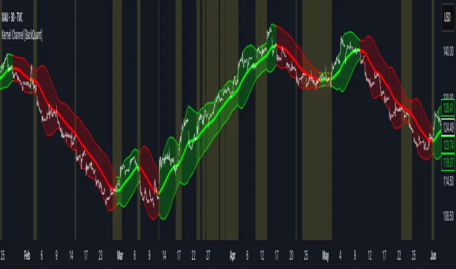
Kernel Channel [BackQuant]Kernel Channel
A non-parametric, kernel-weighted trend channel that adapts to local structure, smooths noise without lagging like moving averages, and highlights volatility compressions, expansions, and directional bias through a flexible choice of kernels, band types, and squeeze logic.
What this is
This indicator builds a full trend channel using kernel regression rather than classical averaging. Instead of a simple moving average or exponential weighting, the midline is computed as a kernel-weighted expectation of past values. This allows it to adapt to local shape, give more weight to nearby bars, and reduce distortion from outliers.
You can think of it as a sliding local smoother where you define both the “window” of influence (Window Length) and the “locality strength” (Bandwidth). The result is a flexible midline with optional upper and lower bands derived from kernel-weighted ATR or kernel-weighted standard deviation, letting you visualize volatility in a structurally consistent way.
Three plotting modes help demonstrate this difference:
When the midline is shown alone, you get a smooth, adaptive baseline that behaves almost like a regression moving average, as shown in this view:
When full channels are enabled, you see how standard deviation reacts to local structure with dynamically widening and tightening bands, a mode illustrated here:
When ATR mode is chosen instead of StdDev, band width reflects breadth of movement rather than variance, creating a volatility-aware envelope like the example here:
Why kernels
Classical moving averages allocate fixed weights. Kernels let the user define weighting shape:
Epanechnikov — emphasizes bars near the current bar, fades fast, stable and smooth.
Triangular — linear decay, simple and responsive.
Laplacian — exponential decay from the current point, sharper reactivity.
Cosine — gentle periodic decay, balanced smoothness for trend filters.
Using these in combination with a bandwidth parameter gives fine control over smoothness vs responsiveness. Smaller bandwidths give sharper local sensitivity, larger bandwidths give smoother curvature.
How it works (core logic)
The indicator computes three building blocks:
1) Kernel-weighted midline
For every bar, a sliding window looks back Window Length bars. Each bar in this window receives a kernel weight depending on:
its index distance from the present
the chosen kernel shape
the bandwidth parameter (locality)
Weights form the denominator, weighted values form the numerator, and the resulting ratio is the kernel regression mean. This midline is the central trend.
2) Kernel-based width
You choose one of two band types:
Kernel ATR — ATR values are kernel-averaged, producing a smooth, volatility-based width that is not dependent on variance. Ideal for directional trend channels and regime separation.
Kernel StdDev — local variance around the midline is computed through kernel weighting. This produces a true statistical envelope that narrows in quiet periods and widens in noisy areas.
Width is scaled using Band Multiplier , controlling how far the envelope extends.
3) Upper and lower channels
Provided midline and width exist, the channel edges are:
Upper = midline + bandMult × width
Lower = midline − bandMult × width
These create smooth structures around price that adapt continuously.
Plotting modes
The indicator supports multiple visual styles depending on what you want to emphasize.
When only the midline is displayed, you get a pure kernel trend: a smooth regression-like curve that reacts to local structure while filtering noise, demonstrated here: This provides a clean read on direction and slope.
With full channels enabled, the behavior of the bands becomes visible. Standard deviation mode creates elastic boundaries that tighten during compressions and widen during turbulence, which you can see in the band-focused demonstration: This helps identify expansion events, volatility clusters, and breakouts.
ATR mode shifts interpretation from statistical variance to raw movement amplitude. This makes channels less sensitive to outliers and more consistent across trend phases, as shown in this ATR variation example: This mode is particularly useful for breakout systems and bar-range regimes.
Regime detection and bar coloring
The slope of the midline defines directional bias:
Up-slope → green
Down-slope → red
Flat → gray
A secondary regime filter compares close to the channel:
Trend Up Strong — close above upper band and midline rising.
Trend Down Strong — close below lower band and midline falling.
Trend Up Weak — close between midline and upper band with rising slope.
Trend Down Weak — close between lower band and midline with falling slope.
Compression mode — squeeze conditions.
Bar coloring is optional and can be toggled for cleaner charts.
Squeeze logic
The indicator includes non-standard squeeze detection based on relative width , defined as:
width / |midline|
This gives a dimensionless measure of how “tight” or “loose” the channel is, normalized for trend level.
A rolling window evaluates the percentile rank of current width relative to past behavior. If the width is in the lowest X% of its last N observations, the script flags a squeeze environment. This highlights compression regions that may precede breakouts or regime shifts.
Deviation highlighting
When using Kernel StdDev mode, you may enable deviation flags that highlight bars where price moves outside the channel:
Above upper band → bullish momentum overextension
Below lower band → bearish momentum overextension
This is turned off in ATR mode because ATR widths do not represent distributional variance.
Alerts included
Kernel Channel Long — midline turns up.
Kernel Channel Short — midline turns down.
Price Crossed Midline — crossover or crossunder of the midline.
Price Above Upper — early momentum expansion.
Price Below Lower — downward volatility expansion.
These help automate regime changes and breakout detection.
How to use it
Trend identification
The midline acts as a bias filter. Rising midline means trend strength upward, falling midline means downward behavior. The channel width contextualizes confidence.
Breakout anticipation
Kernel StdDev compressions highlight areas where price is coiling. Breakouts often follow narrow relative width. ATR mode provides structural expansion cues that are smooth and robust.
Mean reversion
StdDev mode is suitable for fade setups. Moves to outer bands during low volatility often revert to the midline.
Continuation logic
If price breaks above the upper band while midline is rising, the indicator flags strong directional expansion. Same logic for breakdowns on the lower band.
Volatility characterization
Kernel ATR maps raw bar movements and is excellent for identifying regime shifts in markets where variance is unstable.
Tuning guidance
For smoother long-term trend tracking
Larger window (150–300).
Moderate bandwidth (1.0–2.0).
Epanechnikov or Cosine kernel.
ATR mode for stable envelopes.
For swing trading / short-term structure
Window length around 50–100.
Bandwidth 0.6–1.2.
Triangular for speed, Laplacian for sharper reactions.
StdDev bands for precise volatility compression.
For breakout systems
Smaller bandwidth for sharp local detection.
ATR mode for stable envelopes.
Enable squeeze highlighting for identifying setups early.
For mean-reversion systems
Use StdDev bands.
Moderate window length.
Highlight deviations to locate overextended bars.
Settings overview
Kernel Settings
Source
Window Length
Bandwidth
Kernel Type (Epanechnikov, Triangular, Laplacian, Cosine)
Channel Width
Band Type (Kernel ATR or Kernel StdDev)
Band Multiplier
Visuals
Show Bands
Color Bars By Regime
Highlight Squeeze Periods
Highlight Deviation
Lookback and Percentile settings
Colors for uptrend, downtrend, squeeze, flat
Trading applications
Trend filtering — trade only in direction of the midline slope.
Breakout confirmation — expansion outside the bands while slope agrees.
Squeeze timing — compression periods often precede the next directional leg.
Volatility-aware stops — ATR mode makes channel edges suitable for adaptive stop placement.
Structural swing mapping — StdDev bands help locate midline pullbacks vs distributional extremes.
Bias rotation — bar coloring highlights when regime shifts occur.
Notes
The Kernel Channel is not a signal generator by itself, but a structural map. It helps classify trend direction, volatility environment, distribution shape, and compression cycles. Combine it with your entry and exit framework, risk parameters, and higher-timeframe confirmation.
It is designed to behave consistently across markets, to avoid the bluntness of classical averages, and to reveal subtle curvature in price that traditional channels miss. Adjust kernel type, bandwidth, and band source to match the noise profile of your instrument, then use squeeze logic and deviation highlighting to guide timing.
RSI Driven ATR Trend [NeuraAlgo]
RSI Driven ATR Trend
Dynamic Trend Detection and Strength Analysis
Unlock the market’s hidden rhythm with the RSI Driven ATR Trend , a sophisticated tool designed to measure trend direction and strength using a combination of RSI momentum and ATR-based volatility . This indicator provides real-time insights into bullish and bearish phases, helping traders identify potential turning points and optimize entry and exit decisions.
1.Core In Logic:
Dynamically calculates trend levels based on RSI and ATR interactions.
Highlights trend direction with intuitive color coding: green for bullish, red for bearish.
Displays trend strength as a percentage to quantify momentum intensity.
Automatic visual cues for potential trend reversals with “Turn Up” and “Turn Down” labels.
Advanced smoothing and dynamic gating ensure responsive yet stable trend detection.
Compatible with all timeframes and instruments.
2.Inputs Explained:
Rsi Factor: Adjusts the sensitivity of the RSI in trend calculation. Higher values make the trend detection more responsive to momentum changes.
Multiplier: Multiplies the effect of Rsi Factor to fine-tune trend responsiveness.
Bar Back: Number of bars used for peak and dip calculations, determining how far back the indicator looks for trend changes.
Period: Lookback period used in trend gating and ATR calculations.
Source: Price source for calculations (default is close).
Main Colors: Customize bullish and bearish trend colors.
3.How it Works:
The indicator calculates RSI values and ATR-based dynamic ranges to determine upper and lower trend levels.
Trend direction is determined by price crossing above (bullish) or below (bearish) the dynamic trend line.
Trend strength is expressed as a percentage relative to the trend line, helping you assess momentum intensity.
Visual cues like "Turn Up" and "Turn Down" labels indicate potential trend reversals.
Bars are colored dynamically based on trend direction for quick interpretation.
Ideal for traders seeking a clear, actionable view of market trends without the clutter of multiple indicators. RSI Driven ATR Trend translates complex price behavior into an easy-to-read visual guide, helping you make smarter trading decisions.
Happy Trading!

Accumulation And Distribution Zones (Zeiierman)█ Overview
Accumulation And Distribution Zones (Zeiierman) is a structural zone indicator that highlights where the market has recently been absorbing sell pressure (Accumulation) or releasing buy pressure (Distribution).
The indicator tracks a refined sequence of swing highs and lows and measures how these swings tighten, expand, or step directionally. When they form staircase-style structures such as higher lows with compressing highs for Accumulation or lower highs with compressing lows for Distribution, the script marks these areas as shifts in market control.
Once the full pattern completes, the indicator converts it into an Accumulation or Distribution zone. Each zone is based on a confirmed structural sequence rather than a single point, making it more reliable and reflective of actual market behavior.
The indicator can also display a mini-volume profile within each zone and extend POC levels forward, showing where trading activity clustered most. Combined, these features reveal areas where price has recently shown acceptance, absorption, or rejection, helping you understand whether current price action is reacting to, breaking from, or retesting these important structural regions.
█ How It Works
⚪ Swing Structure
The indicator builds its foundation by detecting swing highs and lows using a configurable Swing Detection Window. Each confirmed swing is stored with its price, time, bar index, and direction. If two consecutive swings share the same direction, only the more extreme one is kept. This produces a clean structural sequence that removes noise and keeps only meaningful turning points.
⚪ Accumulation vs Distribution Pattern Logic
Using the refined swing sequence, the script looks for staircase-style formations that signal shifts in control:
Accumulation (bottoming): higher lows combined with compressing highs.
Distribution (topping): lower highs combined with compressing lows.
Two detection modes are available:
Quick for compact 4-swing formations
Slow for broader 6-swing structures
When a full structural pattern completes, the indicator marks the zone and resets the swing buffer for the next formation.
⚪ Volume Profile Construction
The price range between the zone’s upper and lower boundary is divided into several Rows. For every bar within the zone’s swing range, the bar’s volume is added to the appropriate price row.
Volume is classified as:
Bullish volume when close > open
Bearish volume when close < open
Each row is drawn as two horizontal segments (bull and bear), colored with smooth gradients based on your bull/bear color settings. This creates a compact profile that reveals where trading activity is concentrated inside the zone and whether buyers or sellers dominate those price levels.
█ How to Use
The indicator is designed to provide context and confluence, not raw buy/sell signals.
⚪ Spot Fresh Accumulation & Distribution
Use newly printed zones as a map of where the market has recently:
Absorbed selling and formed a floor (Accumulation below price).
Absorbed buying and formed a cap (Distribution above price).
In a trending environment, fresh accumulation zones below price are often areas to watch for pullbacks, while distribution zones above price can act as sell zones or targets.
⚪ Volume Profile
Longer horizontal bars show where the market traded the most volume inside the zone.
Bull-leaning rows inside an accumulation zone often signal strong buying interest during the formation.
Bear-leaning rows inside a distribution zone highlight concentrated selling pressure.
By combining this volume distribution with the zone label and the broader trend context, you can judge whether the structure is more likely to hold, break, or retest as the price approaches it again.
⚪ POC (Point of Control) Trading
Extended POC zones (Regular or Faded) can be treated as dynamic support/resistance rails:
When price revisits a prior accumulation POC and rejects it from above, the level may act as support. When price retests a distribution POC from below and fails to break through, it can act as resistance.
⚪ Combine with Your Own Strategy
The script does not decide direction for you. You get the most value by combining it with:
Your own trend filters (moving averages, higher timeframe structure, volatility measures).
Your preferred entry models (reversal candles, momentum breaks, liquidity grabs, etc.).
Higher-timeframe mapping.
Think of this tool as a map of where the market did meaningful business. You decide how to trade around those areas.
█ Settings
Acc/Dist Ranges – Master switch for drawing all Accumulation and Distribution zones. Turn this off to temporarily hide boxes while leaving supporting logic active.
Pattern – Shows or hides the swing-based pattern outline that formed each zone. Good for structural debugging and education.
Pattern Sensitivity
Quick – more responsive, detects smaller compact structures.
Slow – stricter, focuses on wider and more established zones.
Swing Detection Window – Pivot width used to confirm swing highs and lows. Larger values filter noise and produce bigger zones; smaller values pick up more minor structures.
Volume Profile – Enables the embedded volume profile inside each zone.
Rows – Number of price slices used to aggregate volume in the zone. Higher values give more detail but increase visual density.
Switch Order – Flips the horizontal order of bull vs bear volume segments within each row.
Extend Zones – Behaviour of POC and zone extension:
None – No forward extension.
Faded Zones – Store and draw up to four past POC zones as faded horizontal levels.
Regular Zones – Extend POC boxes forward until price breaks out.
-----------------
Disclaimer
The content provided in my scripts, indicators, ideas, algorithms, and systems is for educational and informational purposes only. It does not constitute financial advice, investment recommendations, or a solicitation to buy or sell any financial instruments. I will not accept liability for any loss or damage, including without limitation any loss of profit, which may arise directly or indirectly from the use of or reliance on such information.
All investments involve risk, and the past performance of a security, industry, sector, market, financial product, trading strategy, backtest, or individual's trading does not guarantee future results or returns. Investors are fully responsible for any investment decisions they make. Such decisions should be based solely on an evaluation of their financial circumstances, investment objectives, risk tolerance, and liquidity needs.

Fractals Trend [BigBeluga]🔵 OVERVIEW
Fractals Trend is a trend-following overlay that leverages fractal swing points to define dynamic support and resistance zones. By storing and averaging recent high and low fractals, it determines trend direction and plots a smooth band that flips depending on market bias—displaying support during uptrends and resistance during downtrends .
🔵 CONCEPTS
Fractal Swings: Fractals are identified using a customizable length. A high fractal forms when the current high is the highest in a range; a low fractal when the current low is the lowest.
Fractal Memory: The indicator keeps a rolling window of recent high and low fractals inside arrays, limited by the user-defined storage quantity.
switch
upperF => FracrtalsUpper.push(high )
lowerF => FracrtalsLower.push(low )
FracrtalsUpper.size() > fCount => FracrtalsUpper.shift()
FracrtalsLower.size() > fCount => FracrtalsLower.shift()
Trend Detection: Price crossing above the average, min/max or median high fractals signals an uptrend; crossing below average, min/max or median low fractals signals a downtrend.
Dynamic Band Plotting: Depending on the trend, the script plots the average of either the upper or lower fractals as a trailing support or resistance line.
Visual Confirmation: Fractal labels appear as triangle markers at highs and lows, providing additional structural context.
🔵 FEATURES
Automatically detects high and low fractals using customizable length.
Stores a defined number of fractals to smooth out noise and reduce false signals.
Flips trend bias dynamically with colored band and smooth transitions.
Plots fractal-based support in bullish trends, resistance in bearish trends.
Triangle markers show real-time fractal highs and lows.
Fully configurable visuals, color themes, and fractal detection logic.
Clean, non-intrusive overlay that works on any market or timeframe.
🔵 HOW TO USE
Use the colored band as a directional filter: green = uptrend (support), orange = downtrend (resistance).
Combine with entry signals or break/retest strategies when price approaches the band.
Use triangle markers to confirm structural swing points.
Adjust Fractals Length to tune sensitivity—shorter values detect quicker shifts, longer values reduce noise.
Change the fractal bands type to adapt trend detection to different market conditions.
Use in conjunction with momentum or volume tools for confluence.
🔵 CONCLUSION
Fractals Trend offers a lightweight, intuitive way to track market bias using price structure alone. Its smart switching logic and clean visuals make it a powerful tool for trend traders seeking structure-based dynamic S/R—without laggy moving averages or overcomplicated signals.

Support & Resistance Zone Hunter [BOSWaves]Support & Resistance Zone Hunter - Dynamic Structural Zones with Real-Time Breakout Intelligence
Overview
The Support & Resistance Zone Hunter is a professional-grade structural mapping framework designed to automatically detect high-probability support and resistance areas in real time. Unlike traditional static levels or manually drawn zones, this system leverages pivot detection, range thresholds, and optional volume validation to create dynamic zones that reflect the true structural architecture of the market.
Zones evolve as price interacts with their boundaries. The first touch of a zone determines its bias - bullish, bearish, or neutral - and the system tracks the full lifecycle of each zone from formation, testing, and bias establishment to potential breakout events. Diamond-shaped breakout signals highlight structurally significant price expansions while filtering noise using a configurable cooldown period.
By visualizing market structure in this way, traders gain a deeper understanding of price behavior, trend momentum, and areas where liquidity and reactive forces are concentrated.
Theoretical Foundation
The Support & Resistance Zone Hunter is built on the premise that meaningful structural zones arise from two core principles:
Pivot-Based Turning Points : Only significant highs and lows that represent actual swings in price are considered.
Contextual Validation : Zones must pass minimum range criteria and optional volume thresholds to ensure their relevance.
Markets naturally generate numerous micro-pivots that do not carry predictive significance. By filtering out minor swings and validating zones against volume and range, the system isolates levels that are more likely to attract future price interaction or act as catalysts for breakout moves.
This framework captures not only where price is likely to react but also the direction of potential pressure, providing a statistically grounded, visually intuitive representation of market structure.
How It Works
The Support & Resistance Zone Hunter constructs zones through a multi-layered process that blends pivot logic, range validation, and real-time bias determination:
1. Pivot Detection Core
The indicator identifies pivot highs and pivot lows using a configurable lookback period. Zones are only considered valid when both a top and bottom pivot are present.
2. Zone Qualification Engine
Prospective zones must satisfy two conditions:
Range Threshold : The distance between pivot high and low must exceed the minimum percentage set by the user.
Volume Requirement : If enabled, the current volume must exceed the 50-period moving average.
Only zones meeting these criteria are drawn, reducing noise and emphasizing high-probability structural levels.
3. Zone Lifecycle
Once a valid top and bottom pivot exist:
The zone is created starting from the pivot formation bar.
Zones remain active until both boundaries have been touched by price.
The first boundary touched establishes bias: resistance first → bullish bias ,support first → bearish bias, neither → neutral.
Inactive zones stop expanding but remain visible historically to maintain a clear structural context.
4. Visual Rendering
Active zones are displayed as filled boxes with color corresponding to their bias. Top, bottom, and midpoint lines are drawn for reference. Once a zone becomes inactive, its lines are removed while the filled box remains as a historical footprint.
5. Breakout Detection
Breakout signals occur when price closes above the top boundary or below the bottom boundary of an active zone. The system applies a cooldown period and requires price to return to the zone since the previous breakout to prevent signal spam. Bullish and bearish breakouts are visually represented by diamond-shaped markers with configurable colors.
Interpretation
The Support & Resistance Zone Hunter provides a structural view of market balance:
Bullish Zones : Form when resistance is tested first, indicating upward pressure and potential continuation.
Bearish Zones : Form when support is tested first, reflecting downward pressure and continuation risk.
Neutral Zones : Fresh zones that have not yet been interacted with, representing undiscovered liquidity.
Breakout Diamonds : Highlight significant structural price expansions, helping traders identify confirmed continuation moves while filtering noise.
Zones do not simply indicate past levels; they dynamically reflect the evolving battle between buyers and sellers, providing actionable context for both trend continuation and reversion strategies.
Strategy Integration
The Support & Resistance Zone Hunter is versatile and can be applied across multiple trading approaches:
Trend Continuation : Use bullish and bearish zones to confirm directional bias. Breakout diamonds indicate structural continuation opportunities.
Reversion Entries : Neutral zones often act as magnets in ranging markets, allowing for high-probability mean-reversion setups.
Breakout Trading : Diamonds mark true structural expansions, reducing false breakout risk and guiding stop placement or momentum entries.
Liquidity Zone Alignment : Combining the indicator with order block, breaker, or volume-based tools helps validate zones against broader market participation.
Technical Implementation Details
Pivot Engine : Two-sided pivot detection based on configurable lookback.
Zone Qualification : Minimum range requirement and optional volume filter.
Bias Logic : Determined by the first boundary touched.
Zone Lifecycle : Active until both boundaries are touched, historical visibility retained.
Breakout Signals : Diamond markers with cooldown filtering and price-return validation.
Visuals : Transparent filled zones with live top, bottom, and midpoint lines.
Suggested Optimal Parameters
Pivot Lookback : 10 - 30 for intraday, 20 - 50 for swing trading.
Minimum Range % : 0.5 - 2% for crypto or indices, 1 - 3% for metals or forex.
Volume Filter : Enable for assets with inconsistent liquidity; disable for consistently liquid markets.
Breakout Cooldown : 5 - 20 bars depending on volatility.
These suggested parameters should be used as a baseline; their effectiveness depends on the asset and timeframe, so fine-tuning is expected for optimal performance.
Performance Characteristics
High Effectiveness:
Markets with clear pivot structure and reliable volume.
Trending symbols with consistent retests.
Assets where zones attract repeated price interaction.
Reduced Effectiveness:
Random walk markets lacking structural pivots.
Low-volatility periods with minimal price reaction.
Assets with irregular volume distribution or erratic price action.
Integration Guidelines
Use zone color as contextual bias rather than a standalone signal.
Combine with structural tools, order blocks, or volume-based indicators for confluence.
Validate zones on higher timeframes to refine lower timeframe entries.
Treat breakout diamonds as confirmation of continuation rather than independent triggers.
Disclaimer
The Support & Resistance Zone Hunter provides structural zone mapping and breakout analytics. It does not predict price movement or guarantee profitability. Success requires disciplined risk management, proper parameter calibration, and integration into a comprehensive trading strategy.
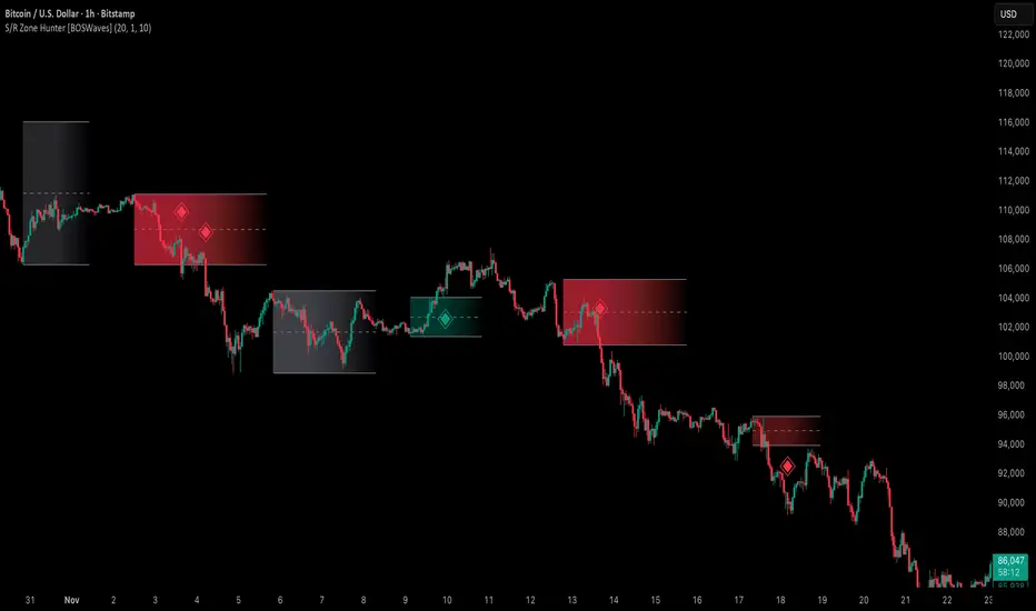
Trend TraderMost trend indicators don’t offer continuation signals or accurate bounce points, so I created this indicator that uses one of the most common trading levels (EMAs). This indicator uses the 50, 100, and 200 EMAs along with WaveTrend signals to trade trends. Buy Signals are filtered so that they only show up when the 100 EMA is above the 200. And Inverse for Sell Signals.
This indicator works well with both Stocks and Crypto. Default settings work best on 15 min, 1H, 2H, and 4H.
(Chart examples are using Heikin Ashi Candles, on Log Scale.)
*Buy and Sell Signals do not repaint.
Settings:
- Ability to show all buy and sell signals regardless of trend.
- To change the sensitivity of the buy and sell signals, change the “Average Length”
- (The lower the number the more sensitive, the higher the number the less they pop up)
- Ability to change EMA Lengths
imgur.com
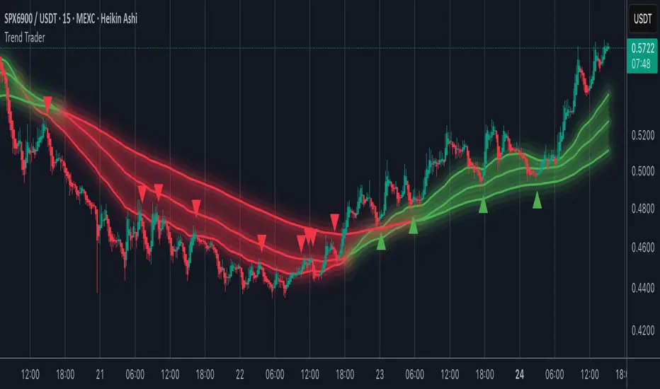
The 'Qualified' POI Scorer [PhenLabs]📊 The “Qualified” POI Scorer (Q-POI)
Version: PineScript™ v6
📌 Description
The “Qualified” POI Scorer helps intermediate traders overcome "analysis paralysis" by filtering Smart Money Concepts (SMC) structures based on their probability. Instead of flooding your chart with every possible Order Block, this script assigns a proprietary “Quality Score” (0-100) to each zone. It analyzes the strength of the displacement, the presence of imbalances (FVG), and liquidity mechanics to determine which zones are worth your attention. It is designed to clean up your charts and enforce discipline by visually fading out low-quality setups.
🚀 Points of Innovation
Dynamic “Glass UI” Transparency that automatically fades weak zones based on their score.
Proprietary Scoring Algorithm (0-100) based on three distinct institutional factors.
Visual Icon System that prints analytical context (💧— 🚀/🐌—🧱) directly on the chart.
Automated Mitigation Tracking that changes the visual state of zones after they are tested.
Displacement Velocity calculation using ATR to verify institutional intent.
🔧 Core Components
Liquidity Sweep Engine: Detects if a pivot point grabbed liquidity from the previous X bars before reversing.
FVG Validator: Checks if the move away from the zone created a valid Fair Value Gap.
Momentum Scorer: Calculates the size of the displacement candle relative to the Average True Range (ATR).
🔥 Key Features
Quality Filtering: Automatically hides or dims zones that score below 50 (user configurable).
State Management: Zones turn grey when mitigated and delete themselves when invalidated.
Visual Scorecard: Displays the exact numeric score on the zone for quick decision-making.
Time-Decay Logic: Keeps the chart clean by managing the lifespan of old zones.
🎨 Visualization
High Score Zones (80-100): Display as bright, semi-solid boxes indicating high probability.
Medium Score Zones (50-79): Display as translucent “glass” boxes.
Low Score Zones (<50): Display as faint “ghost” boxes or are completely hidden.
Rocket Icon (🚀): Indicates high momentum displacement.
Snail Icon (🐌): Indicates low momentum displacement.
Drop Icon (💧): Indicates the zone swept liquidity.
Brick Icon (🧱): Indicates the zone is supported by an FVG.
📖 Usage Guidelines
Swing Structure Length (Default: 5): Controls the sensitivity of the pivot detection; lower numbers create more zones, higher numbers find major swing points.
ATR Length (Default: 14): Determines the lookback period for calculating relative momentum.
Minimum Quality Score (Default: 50): The threshold for which zones are considered “valid” enough to be fully visible.
Bullish/Bearish Colors: Fully customizable colors that adapt their own transparency based on the score.
Show Weak Zones (Default: False): Toggles the visibility of zones that failed the quality check.
✅ Best Use Cases
Filtering noise during high-volatility sessions by focusing only on Score 80+ zones.
Confirming trend continuation entries by looking for the Rocket (🚀) momentum icon.
Avoiding “stale” zones by ignoring any box that has turned grey (Mitigated).
⚠️ Limitations
The indicator is reactive to closed candles and cannot predict news-driven spikes.
Scoring is based on technical structure and does not account for fundamental drivers.
In extremely choppy markets, the ATR filter may produce lower scores due to lack of displacement.
💡 What Makes This Unique
It transforms subjective SMC analysis into an objective, quantifiable score.
The visual hierarchy allows traders to assess chart quality in milliseconds without reading data.
It integrates three separate SMC concepts (Liquidity, Imbalance, Structure) into a single tool.
🔬 How It Works
Step 1: The script identifies a Swing High or Low based on your length input.
Step 2: It looks backward to see if that swing swept liquidity, and looks forward to check for an FVG and displacement.
Step 3: It calculates a weighted score (30pts for Sweep, 30pts for FVG, 40pts for Momentum).
Step 4: It draws the zone with a transparency level designated by the score and appends the relevant icons.
💡 Note:
For the best results, use this indicator on the timeframe you execute trades on (e.g., 15m or 1h). Do not use it to find entries on the 1m chart if your analysis is based on the 4h chart.

Volume Divergence(FULLAUTO)MINHPHUOCKBVolume Divergence( 5 COLOR)
BB50
AUTO TIME
bullishDivergence = color.lime
bearishDivergence =color.red
volSpike =color.rgb
volContraction = color.aqua
incVolTrend =color.new
decVolTrend =color.new
color.rgb

Ultimate Multi-Asset Correlation System by able eiei Ultimate Multi-Asset Correlation System - User Guide
Overview
This advanced TradingView indicator combines WaveTrend oscillator analysis with comprehensive multi-asset correlation tracking. It helps traders understand market relationships, identify regime changes, and spot high-probability trading opportunities across different asset classes.
Key Features
1. WaveTrend Oscillator
Main Signal Lines: WT1 (blue) and WT2 (red) plot momentum and its moving average
Overbought/Oversold Zones: Default levels at +60/-60
Cross Signals:
🟢 Bullish: WT1 crosses above WT2 in oversold territory
🔴 Bearish: WT1 crosses below WT2 in overbought territory
Higher Timeframe (HTF) Analysis: Shows WT1 from 4H, Daily, and Weekly timeframes for trend confirmation
2. Multi-Asset Correlation Tracking
Monitors relationships between:
Major Assets: Gold (XAUUSD), Dollar Index (DXY), US 10-Year Yield, S&P 500
Crypto Assets: Bitcoin, Ethereum, Solana, BNB
Cross-Asset Analysis: Correlation between traditional markets and crypto
3. Market Regime Detection
Automatically identifies market conditions:
Risk-On: High correlation + positive sentiment (🟢 Green background)
Risk-Off: High correlation + negative sentiment (🔴 Red background)
Crypto-Risk-On: Strong crypto correlations (🟠 Orange background)
Low-Correlation: Divergent market behavior (⚪ Gray background)
Neutral: Mixed signals (🟡 Yellow background)
How to Use
Basic Setup
Add to Chart: Apply the indicator to any chart (works on all timeframes)
Choose Display Mode (Display Options):
All: Shows everything (recommended for comprehensive analysis)
WaveTrend Only: Focus on momentum signals
Correlation Only: View market relationships
Heatmap Only: Simplified correlation view
Enable Asset Groups:
✅ Major Assets: Traditional markets (stocks, bonds, commodities)
✅ Crypto Assets: Digital currencies
Mix and match based on your trading focus
Reading the Charts
WaveTrend Section (Bottom Panel)
Above 0 = Bullish momentum
Below 0 = Bearish momentum
Above +60 = Overbought (potential reversal)
Below -60 = Oversold (potential bounce)
Lighter lines = Higher timeframe trends
Correlation Histogram (Colored Bars)
Blue bars: Major asset correlations
Orange bars: Crypto correlations
Purple bars: Cross-asset correlations
Bar height: Correlation strength (-50 to +50 scale)
Background Color
Intensity reflects correlation strength
Color shows market regime
Dashboard Elements
🎯 Market Regime Analysis (Top Left)
Current Regime: Overall market condition
Average Correlation: Strength of relationships (0-1 scale)
Risk Sentiment: -100% (risk-off) to +100% (risk-on)
HTF Alignment: Multi-timeframe trend agreement
Signal Quality: Confidence level for current signals
📊 Correlation Matrix (Top Right)
Shows correlation values between asset pairs:
1.00: Perfect positive correlation
0.75+: Strong correlation (🟢 Green)
0.50+: Medium correlation (🟡 Yellow)
0.25+: Weak correlation (🟠 Orange)
Below 0.25: Negative/no correlation (🔴 Red)
🔥 Correlation Heatmap (Bottom Right)
Visual matrix showing:
Gold vs. DXY, BTC, ETH
DXY vs. BTC, ETH
BTC vs. ETH
Color-coded strength
📈 Performance Tracker (Bottom Left)
Tracks individual asset momentum:
WT1 Values: Current momentum reading
Status: OB (overbought) / OS (oversold) / Normal
Trading Strategies
1. High-Probability Trend Following
✅ Entry Conditions:
WaveTrend bullish/bearish cross
HTF Alignment matches signal direction
Signal Quality > 70%
Correlation supports direction
2. Regime Change Trading
🎯 Watch for regime shifts:
Risk-Off → Risk-On = Consider long positions
High correlation → Low correlation = Reduce position size
Crypto-Risk-On = Focus on crypto longs
3. Divergence Trading
🔍 Look for:
Strong correlation breakdown = Potential volatility
Cross-asset correlation surge = Follow the leader
Volume-price correlation extremes = Trend confirmation
4. Overbought/Oversold Reversals
⚡ Trade reversals when:
WT crosses in extreme zones (-60/+60)
HTF alignment shows opposite trend weakening
Correlation confirms mean reversion setup
Customization Tips
Fine-Tuning Parameters
WaveTrend Core:
Channel Length (10): Lower = more sensitive, Higher = smoother
Average Length (21): Adjust for your timeframe
Correlation Settings:
Length (50): Longer = more stable, Shorter = more responsive
Smoothing (5): Reduce noise in correlation readings
Market Regime:
Risk-On Threshold (0.6): Lower = earlier regime signals
High Correlation Threshold (0.75): Adjust sensitivity
Custom Asset Selection
Replace default symbols with your preferred markets:
Major Assets: Any forex, indices, bonds
Crypto: Any digital currencies
Must use correct exchange prefix (e.g., BINANCE:BTCUSDT)
Alert System
Enable "Advanced Alerts" to receive notifications for:
✅ Market regime changes
✅ Correlation breakdowns/surges
✅ Strong signals with high correlation
✅ Extreme volume-price correlation
✅ Complete HTF alignment
Correlation Interpretation Guide
ValueMeaningTrading Implication+0.75 to +1.0Strong positiveAssets move together+0.5 to +0.75Moderate positiveGenerally aligned+0.25 to +0.5Weak positiveLoose relationship-0.25 to +0.25No correlationIndependent movements-0.5 to -0.25Weak negativeSlight inverse relationship-0.75 to -0.5Moderate negativeTend to move opposite-1.0 to -0.75Strong negativeStrongly inversely correlated
Best Practices
Use Multiple Timeframes: Check HTF alignment before trading
Confirm with Correlation: Strong signals work best with supportive correlations
Watch Regime Changes: Adjust strategy based on market conditions
Volume Matters: Enable volume-price correlation for confirmation
Quality Over Quantity: Trade only high-quality setups (>70% signal quality)
Common Patterns to Watch
🔵 Risk-On Environment:
Gold-BTC positive correlation
DXY negative correlation with risk assets
High crypto correlations
🔴 Risk-Off Environment:
Flight to safety (Gold up, stocks down)
DXY strength
Correlation breakdowns
🟡 Transition Periods:
Low correlation across assets
Mixed HTF signals
Use caution, reduce position sizes
Technical Notes
Calculation Period: Uses HLC3 (average of high, low, close)
Correlation Window: Rolling correlation over specified length
HTF Data: Accurately calculated using security() function
Performance: Optimized for real-time calculation on all timeframes
Support
For optimal performance:
Use on 15-minute to daily timeframes
Enable only needed asset groups
Adjust correlation length based on trading style
Combine with your existing strategy for confirmation
Enjoy comprehensive multi-asset analysis! 🚀

PanjiAlgo V1 [Alpha]PanjjAlgo V1 is a price–action based signal toolkit designed for traders who want clean entries and structured risk management right on the chart.
The script combines engulfing candle patterns, RSI filters, ATR-based volatility and a candle-stability check to highlight high–conviction BUY and SELL zones only when the move is confirmed. To reduce noise, you can optionally disable repeating signals so clusters of overlapping arrows are filtered out.
Each signal automatically generates TP & SL levels based on ATR, with a configurable Risk:Reward ratio (1:1, 2:3, 1:2, 1:4) and a TP/SL multiplier to match your personal risk profile. TP & SL prices are plotted directly on the chart for quick decision-making.
Cosmetic controls allow you to customize label style (text bubble / triangle / arrow), label size and colors so PanjjiAlgo fits seamlessly into your chart layout, whether you are scalping intraday or swing trading higher timeframes.
This script is an experimental alpha version and is intended as a decision-support tool only. It does not guarantee profits and should always be used together with your own analysis and risk management.

Grok/Claude MoneyLine Fusion → Grok/Claude X SeriesMoneyLine Fusion - Quick Description
MoneyLine Fusion is a complete trading system for swing traders and trend followers, designed for volatile assets like Bitcoin, Ethereum, forex pairs, and actively traded stocks across 5-minute to daily timeframes.
How It Works
The indicator combines four technical tools into one system. The MoneyLine (smoothed trend line) shows market direction - green for uptrends, red for downtrends, yellow for choppy markets. Dynamic Bands expand and contract based on volatility, marking support and resistance zones. The Fisher Transform identifies extreme momentum - below -2.0 signals oversold (buy potential), above +2.0 signals overbought (sell potential). The Aroon indicator confirms trend strength.
Signal Generation with TA Score Filter
Buy signals appear when: Fisher drops below -2.0, Aroon Up is below 15%, Aroon Down is above 85%, and the TA Score is ≥+2 (when filter enabled). Sell signals trigger when: Fisher rises above +2.0, Aroon Up exceeds 85%, Aroon Down falls below 15%, and the TA Score is ≤-2 (when filter enabled). Signals display as bright blue candles with BUY or SELL labels showing entry price.
The TA Score (default: OFF) combines MACD, DMI, MFI, and RSI into a composite score from -7 to +7. When enabled with the default ±2 threshold, it requires moderate multi-indicator agreement before signals fire, dramatically reducing false signals in choppy markets. Toggle it on for conservative high-probability trades, or leave it off for more frequent signals. Adjust the threshold from 0-7 to control signal quality versus quantity.
Trading Tips
Trade with the MoneyLine color direction. Check the Info Panel for volatility levels (affects stop placement) and TA Score status. The score displays as colored squares (green=bullish, red=bearish, yellow=mixed, gray=neutral) and in the Info Panel with descriptive text. Customize settings: disable/enable TA Score filter, adjust thresholds, or modify Fisher and Aroon levels. Works best during high-liquidity sessions in trending markets.
Bottom line: Multi-layered confirmation system that signals only when genuine market confluence exists, letting you focus on execution and risk management.
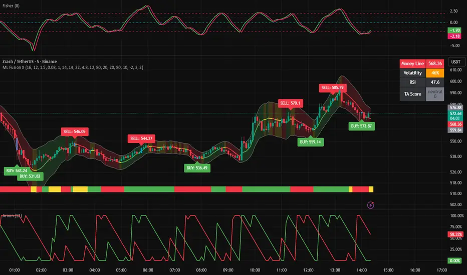
Ultimate Std Dev Channel • 4 Zones • 100% WORKINGStandard-deviation channel — fully customizable (band width, line style, colors, opacity, thickness, and labels).

PanjiAlgo V2 [Alpha]PanjiAlgo V2 is a confluence-based toolkit that combines EMA trend, institutional order blocks, and smart zone visualization in a single indicator.
Core logic:
• Trend Filter – 9-period EMA with optional smoothing (SMA / EMA / RMA / WMA / VWMA) and EMA-based Bollinger Bands to track dynamic structure and volatility.
• Order Blocks – integrated LuxAlgo Order Block Detector logic (used under CC BY-NC-SA 4.0 license) to highlight bullish and bearish institutional zones with extendable boxes and average lines.
• Smart BUY Triggers – BUY labels only appear when price is:
1) Trading above the EMA (trend up),
2) Retracing back into the most recent bullish order block, and
3) Touching or interacting with the EMA at that zone.
This design helps you focus on high-probability pullbacks into institutional demand areas instead of chasing price. PanjiAlgo V2 is a decision-support tool only and does not gu

Filter Ribbon1. Indicator Name
Filter Ribbon
2. One-line Introduction
A trend visualization ribbon that uses linear regression and directional scoring to highlight bullish and bearish strength with intuitive color gradients.
3. General Overview
Filter Ribbon is a minimalistic yet powerful trend visualization tool that leverages linear regression slope ordering to determine directional momentum. It analyzes the ordering of regression values over a defined lookback period and quantifies how consistently the price has been trending upward or downward.
Using a pairwise comparison system, it calculates a trend "score" and compares this to a configurable threshold to determine if a bullish, bearish, or neutral condition exists.
The result is a color-coded ribbon that sits over the chart, changing hue and opacity based on both the direction and strength of the trend. The stronger the directional alignment, the more opaque the ribbon becomes, offering traders a fast, intuitive way to assess market sentiment at a glance.
It also includes an optional linear regression line to further help visualize the central trend.
This indicator is best used in trend-following systems or as a dynamic background layer when combined with signal-based strategies.
Thanks to its efficient design and protected logic, Filter Ribbon offers high-performance visualization without compromising strategy integrity.
4. Key Advantages
🌈 Visual Trend Heatmap
Dynamic color ribbon gives real-time visual feedback on both trend direction and strength.
🔢 Quantified Trend Scoring
Calculates a mathematically sound trend score using pairwise linear regression comparisons.
⚖️ Adjustable Sensitivity
Users can tune lookback and threshold parameters to fit different asset classes and timeframes.
📉 Smooth Ribbon Effect
Plots upper/lower bands around regression line with smooth filling for a professional chart look.
🎯 Precise Trend Confirmation
Acts as a confidence layer for other entry/exit signals by confirming broader trend bias.
🔒 Secure and Minimal Codebase
Core logic is embedded securely with minimal exposure, reducing risk of replication or misuse.
📘 Indicator User Guide
📌 Basic Concept
Filter Ribbon determines trend direction and intensity by comparing the order of linear regression values over time.
It forms a ribbon on the chart that changes color based on trend direction and opacity based on trend strength.
This makes it ideal for identifying clear trending periods vs. uncertain consolidations.
⚙️ Settings Explained
Lookback Period: Number of bars for scoring the trend direction (higher = smoother trend)
Range Tolerance (%): Determines how aggressive the trend classification is (lower = stricter)
Regression Length: Period for calculating the base linear regression line
Ribbon Colors: Customize colors for bullish and bearish conditions
📈 Bullish Timing Example
Ribbon color is green and becomes increasingly opaque
Regression line slopes upward and price remains above it
Can be used as trend confirmation for long trades
📉 Bearish Timing Example
Ribbon color is red with higher opacity
Price consistently below the regression line
Useful for confirming short trade setups or avoiding long entries
🧪 Recommended Use Cases
Combine with breakout indicators to validate if the breakout aligns with broader trend
Use in swing or trend-following strategies as a background filter
Helps filter out trades during unclear, sideways market conditions
🔒 Precautions
Not a signal generator on its own — meant for trend context only
Ribbon may lag slightly during sudden trend reversals; best used with reactive entry tools
Always test ribbon parameters on your specific market/timeframe before applying live
Avoid using solely in low-volatility or flat markets — sensitivity may require tuning
+++
SHIVAJI 1:2 SIMPLE BREAKOUT SETUP - CLEANManage risk reward and use this indicator
Breakout structure auto correct
Volume consider in break out
PanjjiAlgo V1 [Alpha]PanjjAlgo V1 is a price–action based signal toolkit designed for traders who want clean entries and structured risk management right on the chart.
The script combines engulfing candle patterns, RSI filters, ATR-based volatility and a candle-stability check to highlight high–conviction BUY and SELL zones only when the move is confirmed. To reduce noise, you can optionally disable repeating signals so clusters of overlapping arrows are filtered out.
Each signal automatically generates TP & SL levels based on ATR, with a configurable Risk:Reward ratio (1:1, 2:3, 1:2, 1:4) and a TP/SL multiplier to match your personal risk profile. TP & SL prices are plotted directly on the chart for quick decision-making.
Cosmetic controls allow you to customize label style (text bubble / triangle / arrow), label size and colors so PanjjiAlgo fits seamlessly into your chart layout, whether you are scalping intraday or swing trading higher timeframes.
This script is an experimental alpha version and is intended as a decision-support tool only. It does not guarantee profits and should always be used together with your own analysis and risk management.

Bollinger Band with Clouds, MA, and Selectable Buy/Sell AlertsBollinger Bands + Clouds + Multi-TF Signals — All in One Open-Source Indicator
This open-source indicator combines multiple technical tools into a single, flexible charting solution — giving traders clear context and the ability to customize or build upon the code. Perfect for intraday, swing, or longer-term analysis.
What it includes:
NMA (Normalized Moving Average): Adaptive, multi-length moving average for trend visualization.
VWAP: Volume-weighted average price for intraday anchoring.
Bollinger Bands: Customizable upper/lower bands with baseline and fill, providing dynamic volatility context.
Hull Moving Average + Kalman Filter: Smoothed trend detection with optional buy/sell shapes on crossovers.
Multi-Timeframe EMAs: Short, medium, and long-term EMAs from multiple timeframes, all in one view.
RSI & ATR: Optional visibility to track momentum and volatility.
Customizable Colors & Transparency: Every line, fill, and shape can be adjusted independently.
Selectable Buy/Sell Alerts: Configurable shapes and TradingView alert conditions for strategy observation.
Why you’ll love it:
Fully open-source: inspect, modify, and adapt the code for your own analysis.
Clean, informative visualizations that consolidate multiple indicators without cluttering your chart.
Flexible for intraday, swing, or longer-term timeframes.
Team Player Friendly:
This script is intentionally published as open-source to support the TradingView community. All code is fully visible — no proprietary sections — so anyone can learn from, modify, and contribute to the indicator.
Disclaimer:
This indicator is for informational purposes only. It does not constitute financial, trading, or investment advice. Users should conduct their own analysis before making trading decisions.

EMA Trend Pro v5.0 5M ONLY — 策略版(1:1出30%+保本)Here is a clear, professional English description you can copy-paste directly (suitable for sharing with friends, investors, brokers, or posting on TradingView):
EMA Trend Pro v5.0 – Strategy Overview
This is a trend-following strategy designed for 15-minute charts on assets like XAUUSD, NASDAQ, BTC, and ETH.
Entry Rules
Buy when the 7, 14, and 21-period EMAs are aligned upward and the 14-period EMA crosses above the 144-period EMA (with ADX > 20 and volume confirmation).
Sell short when the EMAs are aligned downward and the 14-period EMA crosses below the 144-period EMA.
Risk Management
Initial stop-loss is placed at 1.8 × ATR below (long) or above (short) the entry price.
Position size is calculated to risk a fixed percentage of equity per trade.
Profit-Taking & Trade Management
When price reaches 1:1 reward-to-risk, 30% of the position is closed.
At the same moment, the stop-loss for the remaining 70% is moved to the entry price (breakeven).
The remaining position is split:
50% targets 1:2 reward-to-risk
50% targets 1:3 reward-to-risk (allowing big wins during strong trends)
Visualization
Clean colored bars extend to the right showing entry, stop-loss, and three take-profit levels.
Price labels clearly display "Entry", "SL", "TP1 1:1", "TP2 1:2", and "TP3 1:3".
Only the current trade is displayed for a clean chart.
Key Advantages
High win rate due to breakeven protection after 1R
Excellent reward-to-risk ratio that lets winners run
Fully automated, works on any market with clear trends
Professional look, easy to understand and explain
Perfect for swing traders who want consistent profits with limited downside risk.
Feel free to use this description on TradingView, in your trading journal, or when explaining the strategy to others!
If you want a shorter version (e.g., for TradingView description box) or a Chinese version, just let me know — I’ll give it to you right away! 😊

Market Sentiment [NeuraAlgo]
Market Sentiment
This indicator provides a real-time view of market momentum and sentiment by analyzing bullish and bearish impulses using price and volatility-based calculations. It visualizes trends on the chart and offers a dashboard with key statistics.
1.Status Calculation
The Status measures bullish momentum by identifying strong upward impulses.
Equation:
Status Source = Average of lows where(Low - High ) > ATR
For each bar, it checks if the current low minus the high from two bars ago exceeds the Average True Range (ATR) .
All lows that satisfy this condition are collected.
The average of these lows forms the Status Source , representing the level of strong buying pressure.
This helps traders visualize where significant bullish activity is concentrated and gauge upward momentum.
2.Status Source Calculation
Similarly, bearish impulses are detected by checking if highs fall below lows from two bars ago beyond ATR thresholds. The corresponding levels form the reference for selling pressure.
3. Trend Strength and States
Strength is Quantifies how far the price is from bullish or bearish reference levels as a percentage.
Trend States
Stability Phase (Gray): Market is quiet, minimal momentum.
Positive Flow (Green): Bullish pressure dominates; buyers are in control.
Negative Flow (Red): Bearish pressure dominates; sellers lead.
State Transition: Market is shifting; momentum is building.
4. Visuals
Bar colors indicate trend state: green for bullish, red for bearish, gray for neutral.
Filled zones highlight bullish and bearish reference levels for intuitive trend analysis.
5. Dashboard
An optional dashboard displays:
Sentiment: Visual gradient representing bullish or bearish dominance.
Status: Current trend state in concise, human-readable terms.
6. Purpose:
This indicator is designed to identify the current market status and the behavior of the asset by analyzing bullish and bearish impulses. It helps traders understand whether the market shows signs of stability, growth, or decline based on the asset’s price action and volatility.
Understand the asset behavior
Healthy asset behavior
Weak asset behavior
Market Sentiment combines price action, ATR-based volatility, and impulse tracking to provide a clear and actionable view of market conditions. The BullLine equation ensures that only meaningful bullish moves are highlighted, giving traders a reliable reference for momentum and potential entry points.

ATR STRUCTURESTATIC LINES SET BY ATR VALUES AND MULTIPLED OBSE$RVED EPERCENTAGES more of a tool I use for me then it is for anyone else.