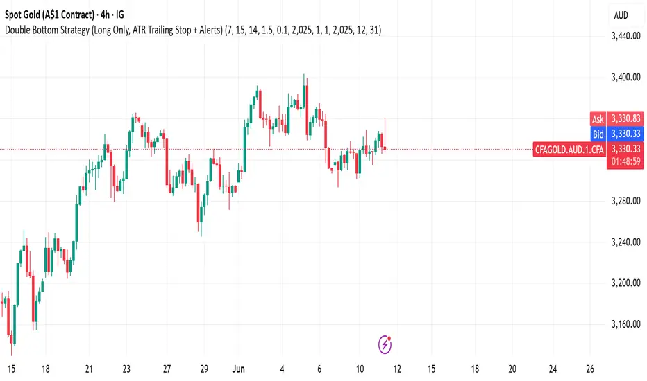
Backtesting ModuleDo you often find yourself creating new 'strategy()' scripts for each trading system? Are you unable to focus on generating new systems due to fatigue and time loss incurred in the process? Here's a potential solution: the 'Backtesting Module' :)
INTRODUCTION
Every trading system is based on four basic conditions: long entry, long exit, short entry and short exit (which are typically defined as boolean series in Pine Script).
If you can define the conditions generated by your trading system as a series of integers, it becomes possible to use these variables in different scripts in efficient ways. (Pine Script is a convenient language that allows you to use the integer output of one indicator as a source in another.)
The 'Backtesting Module' is a dynamic strategy script designed to adapt to your signals. It boasts two notable features:
⮞ It produces a backtest report using the entry and exit variables you define.
⮞ It not only serves for system testing but also to combine independent signals into a single system. (This functionality enables to create complex strategies and report on their success!)
The module tests Golden and Death cross signals by default, when you enter your own conditions the default signals will be neutralized. The methodology is described below.
PREPARATION
There are three simple steps to connect your own indicator to the Module.
STEP 1
Firstly, you must define entry and exit variables in your own script. Let's elucidate it with a straightforward example. Consider a system generating long and short signals based on the intersections of two moving averages. Consequently, our conditions would be as follows:
// Signals
long = ta.crossover(ta.sma(close, 14), ta.sma(close, 28))
short = ta.crossunder(ta.sma(close, 14), ta.sma(close, 28))
Now, the question is: How can we convert boolean variables into integer variables? The answer is conditional ternary block, defined as follows:
// Entry & Exit
long_entry = long ? 1 : 0
long_exit = short ? 1 : 0
short_entry = short ? 1 : 0
short_exit = long ? 1 : 0
The mechanics of the Entry & Exit variables are simple. The variable takes on a value of 1 when your trading system generates the signal and if your system does not produce any signal, variable returns 0. In this example, you see how exit signals can be generated in a trading system that only contains entry signals. If you have a system with original exit signals, you can also use them directly. (Please mind the NOTES section below).
STEP 2
To utilize the Entry & Exit variables as source in another script, they must be plotted on the chart. Therefore, the final detail to include in the script containing your trading system would be as follows:
// Plot The Output
plot(long_entry, "Long Entry", display=display.data_window, editable=false)
plot(long_exit, "Long Exit", display=display.data_window, editable=false)
plot(short_entry, "Short Entry", display=display.data_window, editable=false)
plot(short_exit, "Short Exit", display=display.data_window, editable=false)
STEP 3
Now, we are ready to test the system! Load the Backtesting Module indicator onto the chart along with your trading system/indicator. Then set the outputs of your system (Long Entry, Long Exit, Short Entry, Short Exit) as source in the module. That's it.
FEATURES & ORIGINALITY
⮞ Primarily, this script has been created to provide you with an easy and practical method when testing your trading system.
⮞ I thought it might be nice to visualize a few useful results. The Backtesting Module provides insights into the outcomes of both long and short trades by computing the number of trades and the success percentage.
⮞ Through the 'Trade' parameter, users can specify the market direction in which the indicator is permitted to initiate positions.
⮞ Users have the flexibility to define the date range for the test.
⮞ There are optional features allowing users to plot entry prices on the chart and customize bar colors.
⮞ The report and the test date range are presented in a table on the chart screen. The entry price can be monitored in the data window.
⮞ Note that results are based on realized returns, and the open trade is not included in the displayed results. (The only exception is the 'Unrealized PNL' result in the table.)
STRATEGY SETTINGS
The default parameters are as follows:
⮞ Initial Balance : 10000 (in units of currency)
⮞ Quantity : 10% of equity
⮞ Commission : 0.04%
⮞ Slippage : 0
⮞ Dataset : All bars in the chart
For a realistic backtest result, you should size trades to only risk sustainable amounts of equity. Do not risk more than 5-10% on a trade. And ALWAYS configure your commission and slippage parameters according to pessimistic scenarios!
NOTES
⮞ This script is intended solely for development purposes. And it'll will be available for all the indicators I publish.
⮞ In this version of the module, all order types are designed as market orders. The exit size is the sum of the entry size.
⮞ As your trading conditions grow more intricate, you might need to define the outputs of your system in alternative ways. The method outlined in this description is tailored for straightforward signal structures.
⮞ Additionally, depending on the structure of your trading system, the backtest module may require further development. This encompasses stop-loss, take-profit, specific exit orders, quantity, margin and risk management calculations. I am considering releasing improvements that consider these options in future versions.
⮞ An example of how complex trading signals can be generated is the OTT Collection. If you're interested in seeing how the signals are constructed, you can use the link below.
THANKS
Special thanks to PineCoders for their valuable moderation efforts.
I hope this will be a useful example for the TradingView community...
DISCLAIMER
This is just an indicator, nothing more. It is provided for informational and educational purposes exclusively. The utilization of this script does not constitute professional or financial advice. The user solely bears the responsibility for risks associated with script usage. Do not forget to manage your risk. And trade as safely as possible. Best of luck!
Strategy!
RMI Trend Sync - Strategy [presentTrading]█ Introduction and How It Is Different
The "RMI Trend Sync - Strategy " combines the strength of the Relative Momentum Index (RMI) with the dynamic nature of the Supertrend indicator. This strategy diverges from traditional methodologies by incorporating a dual analytical framework, leveraging both momentum and trend indicators to offer a more holistic market perspective. The integration of the RMI provides an enhanced understanding of market momentum, while the Super Trend indicator offers clear insights into the end of market trends, making this strategy particularly effective in diverse market conditions.
BTC 4h long/short performance
█ Strategy: How It Works - Detailed Explanation
- Understanding the Relative Momentum Index (RMI)
The Relative Momentum Index (RMI) is an adaptation of the traditional Relative Strength Index (RSI), designed to measure the momentum of price movements over a specified period. While RSI focuses on the speed and change of price movements, RMI incorporates the direction and magnitude of those movements, offering a more nuanced view of market momentum.
- Principle of RMI
Calculation Method: RMI is calculated by first determining the average gain and average loss over a given period (Length). It differs from RSI in that it uses the price change (close-to-close) rather than absolute gains or losses. The average gain is divided by the average loss, and this ratio is then normalized to fit within a 0-100 scale.
- Momentum Analysis in the Strategy
Thresholds for Decision Making: The strategy uses predetermined thresholds (pmom for positive momentum and nmom for negative momentum) to trigger trading decisions. When RMI crosses above the positive threshold and other conditions align (e.g., a bullish trend), it signals a potential long entry. Similarly, crossing below the negative threshold in a bearish trend may trigger a short entry.
- Super Trend and Trend Analysis
The Super Trend indicator is calculated based on a higher time frame, providing a broader view of the market trend. This indicator uses the Average True Range (ATR) to adapt to market volatility, making it an effective tool for identifying trend reversals.
The strategy employs a Volume Weighted Moving Average (VWMA) alongside the Super Trend, enhancing its capability to identify significant trend shifts.
ETH 4hr long/short performance
█ Trade Direction
The strategy offers flexibility in selecting the trading direction: long, short, or both. This versatility allows traders to adapt to their market outlook and risk tolerance, whether looking to capitalize on bullish trends, bearish trends, or a combination of both.
█ Usage
To effectively use the "RMI Trend Sync" strategy, traders should first set their preferred trading direction and adjust the RMI and Super Trend parameters according to their risk appetite and trading goals.
The strategy is designed to adapt to various market conditions, making it suitable for different asset classes and time frames.
█ Default Settings
RMI Settings: Length: 21, Positive Momentum Threshold: 70, Negative Momentum Threshold: 30
Super Trend Settings: Length: 10, Higher Time Frame: 480 minutes, Super Trend Factor: 3.5, MA Source: WMA
Visual Settings: Display Range MA: True, Bullish Color: #00bcd4, Bearish Color: #ff5252
Additional Settings: Band Length: 30, RWMA Length: 20
Captain Backtest Model [TFO]Created by @imjesstwoone and @mickey1984, this trade model attempts to capture the expansion from the 10:00-14:00 EST 4h candle using just 3 simple steps. All of the information presented in this description has been outlined by its creators, all I did was translate it to Pine Script. All core settings of the trade model may be edited so that users can test several variations, however this description will cover its default, intended behavior using NQ 5m as an example.
Step 1 is to identify our Price Range. In this case, we are concerned with the highest high and the lowest low created from 6:00-10:00 EST.
Step 2 is to wait for either the high or low of said range to be taken out. Whichever side gets taken first determines the long/short bias for the remainder of the Trade Window (i.e. if price takes the range high, bias is long, and vice versa). Bias must be determined by 11:15 EST, otherwise no trades will be taken. This filter is intended to weed out "choppy" trading days.
Step 3 is to wait for a retracement and enter with a close through the previous candle's high (if long biased) or low (if short biased). There are a couple toggleable criteria that we use to define a retracement; one is checking for opposite close candles that indicate a pullback; another is checking if price took the previous candle's low (if long biased) or high (if short biased).
This trade model was initially tested for index futures, particularly ES and NQ, using a 5m chart, however this indicator allows us to backtest any symbol on any timeframe. Creators @imjesstwoone and @mickey1984 specified a 5 point stop loss on ES and a 25 point stop loss on NQ with their testing.
I've personally found some success in backtesting NQ 5m using a 25 point stop loss and 75 point profit target (3:1 R). Enabling the Use Fixed R:R parameter will ensure that these stops and targets are utilized, otherwise it will enter and hold the position until the close of the Trade Window.
Martingale + Grid DCA Strategy [YinYangAlgorithms]This Strategy focuses on strategically Martingaling when the price has dropped X% from your current Dollar Cost Average (DCA). When it does Martingale, it will create a Purchase Grid around this location to likewise attempt to get you a better DCA. Likewise following the Martingale strategy, it will sell when your Profit has hit your target of X%.
Martingale may be an effective way to lower your DCA. This is due to the fact that if your initial purchase; or in our case, initial Grid, all went through and the price kept going down afterwards, that you may purchase more to help lower your DCA even more. By doing so, you may bring your DCA down and effectively may make it easier and quicker to reach your target profit %.
Grid trading may be an effective way of reducing risk and lowering your DCA as you are spreading your purchases out over multiple different locations. Likewise we offer the ability to ‘Stack Grids’. What this means, is that if a single bar was to go through 20 grids, the purchase amount would be 20x what each grid is valued at. This may help get you a lower DCA as rather than creating 20 purchase orders at each grid location, we create a single purchase order at the lowest grid location, but for 20x the amount.
By combining both Martingale and Grid DCA techniques we attempt to lower your DCA strategically until you have reached your target profit %.
Before we start, we just want to make it known that first off, this Strategy features 8% Commission Fees, you may change this in the Settings to better reflect the Commission Fees of your exchange. On a similar note, due to Commission Fees being one of the number one profit killers in fast swing trade strategies, this strategy doesn’t focus on low trades, but the ideology of it may result in low amounts of trades. Please keep in mind this is not a bad thing. Since it has the ability to ‘Stack Grid Purchases’ it may purchase more for less and result in more profit, less commission fees, and likewise less # of trades.
Tutorial:
In this example above, we have it set so we Martingale twice, and we use 100 grids between the upper and lower level of each martingale; for a total of 200 Grids. This strategy will take total capital (initial capital + net profit) and divide it by the amount of grids. This will result in the $ amount purchased per grid. For instance, say you started with $10,000 and you’ve made $2000 from this Strategy so far, your total capital is $12,000. If you likewise are implementing 200 grids within your Strategy, this will result in $12,000 / 200 = $60 per grid. However, please note, that the further down the grid / martingale is, the more volume it is able to purchase for $60.
The white line within the Strategy represents your DCA. As the Strategy makes purchases, this will continue to get lower as will your Target Profit price (Blue Line). When the Close goes above your Target Profit price, the Strategy will close all open positions and claim the profit. This profit is then reinvested back into the Strategy, which may exponentially help the Strategy become more profitable the longer it runs for.
In the example above, we’ve zoomed in on the first example. In this we want to focus on how the Strategy got back into the trades shortly after it sold. Currently within the Settings we have it set so our entry is when the Lowest with a length of 3 is less than the previous Lowest with a length of 3. This is 100% customizable and there are multiple different entry options you can choose from and customize such as:
EMA 7 Crossover EMA 21
EMA 7 Crossunder EMA 21
RSI 14 Crossover RSI MA 14
RSI 14 Crossunder RSI MA 14
MFI 14 Crossover MFI MA 14
MFI 14 Crossunder MFI MA 14
Lowest of X Length < Previous Lowest of X Length
Highest of X Length > Previous Highest of X Length
All of these entry options may be tailored to be checked for on a different Time Frame than the one you are currently using the Strategy on. For instance, you may be running the Strategy on the 15 minute Time Frame yet decide you want the RSI to cross over the RSI MA on the 1 Day to be a valid entry location.
Please keep in mind, this Strategy focuses on DCA, this means you may not want the initial purchase to be the best location. You may want to buy when others think it is a good time to sell. This is because there may be strong bearish momentum which drives the price down drastically and potentially getting you a good DCA before it corrects back up.
We will continue to add more Entry options as time goes on, and if you have any in mind please don’t hesitate to let us know.
Now, back to the example above, if we refer to the Yellow circle, you may see that the Lowest of a length of 3 was less than its previous lowest, this triggered the martingales to create their grids. Only a few bars later, the price went into the first grid and went a little lower than its midpoint (Yellow line). This caused about 60% of the first grid to be purchased. Shortly after the price went even lower into this grid and caused the entire first martingale grid to be purchased. However, if you notice, the white line (your DCA) is lower than the midpoint of the first grid. This is due to the fact that we have ‘Stack Grid Purchases’ enabled. This allows the Strategy to purchase more when a single bar crosses through multiple grid locations; and effectively may lower your average more than if it simply executed a purchase order at each grid.
Still looking at the same location within our next example, if we simply increase the Martingale amount from 2 to 3 we can see something strange happens. What happened is our Target Profit price was reached, then our entry condition was met, which caused all of the martingale grids to be formed; however, the price continued to increase afterwards. This may not be a good thing, sure the price could correct back down to these grid locations, but what if it didn’t and it just kept increasing? This would result in this Strategy being stuck and unable to make any trades. For this reason we have implemented a Failsafe in the Settings called ‘Reset Grids if no purchase happens after X bars’.
We have enabled our Failsafe ‘Reset Grids if no purchase happens after X bars’ in this example above. By default it is set to 100 bars, but you can change this to whatever works best for you. If you set it to 0, this Failsafe will be disabled and act like the example prior where it is possible to be stuck with no trades executing.
This Failsafe may be an important way to ensure the Strategy is able to make purchases, however it may also mean the Grids increase in price when it is used, and if a massive correction were to occur afterwards, you may lose out on potential profit.
This Strategy was designed with WebHooks in mind. WebHooks allow you to send signals from the Strategy to your exchange. Simply set up a Custom TradingView Bot within the OKX exchange or 3Commas platform (which has your exchange API), enter the data required from the bot into the settings here, select your bot type in ‘Webhook Alert Type’, and then set up the alert. After that you’re good to go and this Strategy will fully automate all of its trades within your exchange for you. You need to format the Alert a certain way for it to work, which we will go over in the next example.
Add an alert for this Strategy and simply modify the alert message so all it says is:
{{strategy.order.alert_message}}
Likewise change from the Alert ‘Settings’ to Alert ‘Notifications’ at the top of the alert popup. Within the Notifications we will enable ‘Webhook URL’ and then we will pass the URL we are sending the Webhook to. In this example we’ve put OKX exchange Webhook URL, however if you are using 3Commas you’ll need to change this to theirs.
OKX Webhook URL:
www.okx.com
3Commas Webhook URL:
app.3commas.io
Make sure you click ‘Create’ to actually create this alert. After that you’re all set! There are many Tutorials videos you can watch if you are still a little confused as to how Webhook trading works.
Due to the nature of this Strategy and how it is designed to work, it has the ability to never sell unless there it will make profit. However, because of this it also may be stuck waiting in trades for quite a long period of time (usually a few months); especially when your Target Profit % is 15% like in the example above. However, this example above may be a good indication that it may maintain profitability for a long period of time; considering this ‘Deep Backtest’ is from 2017-8-17.
We will conclude the tutorial here. Hopefully you understand how this Strategy has the potential to make calculated and strategic DCA Grid purchases for you and then based on a traditional Martingale fashion, bulk sell at the desired Target Profit Percent.
Settings:
Purchase Settings:
Only Purchase if its lower than DCA: Generally speaking, we want to lower our Average, and therefore it makes sense to only buy when the close is lower than our current DCA and a Purchase Condition is met.
Purchase Condition: When creating the initial buy location you must remember, you want to Buy when others are Fearful and Sell when others are Greedy. Therefore, many of the Buy conditions involve times many would likewise Sell. This is one of the bonuses to using a Strategy like this as it will attempt to get you a good entry location at times people are selling.
Lower / Upper Change Length: This Lower / Upper Length is only used if the Purchase Condition is set to 'Lower Changed' or 'Upper Changed'. This is when the Lowest or Highest of this length changes. Lowest would become lower or Highest would become higher.
Purchase Resolution: Purchase Resolution is the Time Frame that the Purchase Condition is calculated on. For instance, you may only want to start a new Purchase Order when the RSI Crosses RSI MA on the 1 Day, but yet you run this Strategy on the 15 minutes.
Sell Settings:
Trailing Take Profit: Trailing Take Profit is where once your Target Profit Percent has been hit, this will trail up to attempt to claim even more profit.
Target Profit Percent: What is your Target Profit Percent? The Strategy will close all positions when the close price is greater than your DCA * this Target Profit Percent.
Grid Settings:
Stack Grid Purchases: If a close goes through multiple Buy Grids in one bar, should we amplify its purchase amount based on how many grids it went through?
Reset Grids if no purchase happens after X Bars: Set this to 0 if you never want to reset. This is very useful in case the price is very bullish and continues to increase after our Target Profit location is hit. What may happen is, Target Profit location is hit, then the Entry condition is met but the price just keeps increasing afterwards. We may not want to be sitting waiting for the price to drop, which may never happen. This is more of a failsafe if anything. You may set it very large, like 500+ if you only want to use it in extreme situations.
Grid % Less than Initial Purchase Price: How big should our Buy Grid be? For instance if we bought at 0.25 and this value is set to 20%, that means our Buy Grid spans from 0.2 - 0.25.
Grid Amounts: How many Grids should we create within our Buy location?
Martingale Settings:
Amount of Times 'Planned' to Martingale: The more Grids + the More Martingales = the less $ spent per grid, however the less risk. Remember it may be better to be right and take your time than risk too much and be stuck too long.
Martingale Percent: When the current price is this percent less than our DCA, lets create another Buy Grid so we can lower our average more. This will make our profit location less.
Webhook Alerts:
Webhook Alert Type: How should we format this Alert? 3Commas and OKX take their alerts differently, so please select the proper one or your webhooks won't work.
3Commas Webhook Alerts:
3Commas Bot ID: The 3Commas Bot ID is needed so we know which BOT ID we are sending this webhook too.
3Commas Email Token: The 3Commas Email Token is needed for your webhooks to work properly as it is linked to your account.
OKX Webhook Alerts:
OKX Signal Token: This Signal Token is attached to your OKX bot and will be used to access it within OKX.
If you have any questions, comments, ideas or concerns please don't hesitate to contact us.
HAPPY TRADING!
Machine Learning: Donchian DCA Grid Strategy [YinYangAlgorithms]This strategy uses a Machine Learning approach on the Donchian Channels with a DCA and Grid purchase/sell Strategy. Not only that, but it uses a custom Bollinger calculation to determine its Basis which is used as a mild sell location. This strategy is a pure DCA strategy in the sense that no shorts are used and theoretically it can be used in webhooks on most exchanges as it’s only using Spot Orders. The idea behind this strategy is we utilize both the Highest Highs and Lowest Lows within a Machine Learning standpoint to create Buy and Sell zones. We then fraction these zones off into pieces to create Grids. This allows us to ‘micro’ purchase as it enters these zones and likewise ‘micro’ sell as it goes up into the upper (sell) zones.
You have the option to set how many grids are used, by default we use 100 with max 1000. These grids can be ‘stacked’ together if a single bar is to go through multiple at the same time. For instance, if a bar goes through 30 grids in one bar, it will have a buy/sell power of 30x. Stacking Grid Buy and (sometimes) Sells is a very crucial part of this strategy that allows it to purchase multitudes during crashes and capitalize on sales during massive pumps.
With the grids, you’ll notice there is a middle line within the upper and lower part that makes the grid. As a Purchase Type within our Settings this is identified as ‘Middle of Zone Purchase Amount In USDT’. The middle of the grid may act as the strongest grid location (aside from maybe the bottom). Therefore there is a specific purchase amount for this Grid location.
This DCA Strategy also features two other purchase methods. Most importantly is its ‘Purchase More’ type. Essentially it will attempt to purchase when the Highest High or Lowest Low moves outside of the Outer band. For instance, the Lowest Low becomes Lower or the Higher High becomes Higher. When this happens may be a good time to buy as it is featuring a new High or Low over an extended period.
The last but not least Purchase type within this Strategy is what we call a ‘Strong Buy’. The reason for this is its verified by the following:
The outer bounds have been pushed (what causes a ‘Purchase More’)
The Price has crossed over the EMA 21
It has been verified through MACD, RSI or MACD Historical (Delta) using Regular and Hidden Divergence (Note, only 1 of these verifications is required and it can be any).
By default we don’t have Purchase Amount for ‘Strong Buy’ set, but that doesn’t mean it can’t be viable, it simply means we have only seen a few pairs where it actually proved more profitable allocating money there rather than just increasing the purchase amount for ‘Purchase More’ or ‘Grids’.
Now that you understand where we BUY, we should discuss when we SELL.
This Strategy features 3 crucial sell locations, and we will discuss each individually as they are very important.
1. ‘Sell Some At’: Here there are 4 different options, by default its set to ‘Both’ but you can change it around if you want. Your options are:
‘Both’ - You will sell some at both locations. The amount sold is the % used at ‘Sell Some %’.
‘Basis Line’ - You will sell some when the price crosses over the Basis Line. The amount sold is the % used at ‘Sell Some %’.
‘Percent’ - You will sell some when the Close is >= X% between the Lower Inner and Upper Inner Zone.
‘None’ - This simply means don’t ever Sell Some.
2. Sell Grids. Sell Grids are exactly like purchase grids and feature the same amount of grids. You also have the ability to ‘Stack Grid Sells’, which basically means if a bar moves multiple grids, it will stack the amount % wise you will sell, rather than just selling the default amount. Sell Grids use a DCA logic but for selling, which we deem may help adjust risk/reward ratio for selling, especially if there is slow but consistent bullish movement. It causes these grids to constantly push up and therefore when the close is greater than them, accrue more profit.
3. Take Profit. Take profit occurs when the close first goes above the Take Profit location (Teal Line) and then Closes below it. When Take Profit occurs, ALL POSITIONS WILL BE SOLD. What may happen is the price enters the Sell Grid, doesn’t go all the way to the top ‘Exiting it’ and then crashes back down and closes below the Take Profit. Take Profit is a strong location which generally represents a strong profit location, and that a strong momentum has changed which may cause the price to revert back to the buy grid zone.
Keep in mind, if you have (by default) ‘Only Sell If Profit’ toggled, all sell locations will only create sell orders when it is profitable to do so. Just cause it may be a good time to sell, doesn’t mean based on your DCA it is. In our opinion, only selling when it is profitable to do so is a key part of the DCA purchase strategy.
You likewise have the ability to ‘Only Buy If Lower than DCA’, which is likewise by default. These two help keep the Yin and Yang by balancing each other out where you’re only purchasing and selling when it makes logical sense too, even if that involves ignoring a signal and waiting for a better opportunity.
Tutorial:
Like most of our Strategies, we try to capitalize on lower Time Frames, generally the 15 minutes so we may find optimal entry and exit locations while still maintaining a strong correlation to trend patterns.
First off, let’s discuss examples of how this Strategy works prior to applying Machine Learning (enabled by default).
In this example above we have disabled the showing of ‘Potential Buy and Sell Signals’ so as to declutter the example. In here you can see where actual trades had gone through for both buying and selling and get an idea of how the strategy works. We also have disabled Machine Learning for this example so you can see the hard lines created by the Donchian Channel. You can also see how the Basis line ‘white line’ may act as a good location to ‘Sell Some’ and that it moves quite irregularly compared to the Donchian Channel. This is due to the fact that it is based on two custom Bollinger Bands to create the basis line.
Here we zoomed out even further and moved back a bit to where there were dense clusters of buy and sell orders. Sometimes when the price is rather volatile you’ll see it ‘Ping Pong’ back and forth between the buy and sell zones quite quickly. This may be very good for your trades and profit as a whole, especially if ‘Only Buy If Lower Than DCA’ and ‘Only Sell If Profit’ are both enabled; as these toggles will ensure you are:
Always lowering your Average when buying
Always making profit when selling
By default 8% commission is added to the Strategy as well, to simulate the cost effects of if these trades were taking place on an actual exchange.
In this example we also turned on the visuals for our ‘Purchase More’ (orange line) and ‘Take Profit’ (teal line) locations. These are crucial locations. The Purchase More makes purchases when the bottom of the grid has been moved (may dictate strong price movement has occurred and may be potential for correction). Our Take Profit may help secure profit when a momentum change is happening and all of the Sell Grids weren’t able to be used.
In the example above we’ve enabled Buy and Sell Signals so that you can see where the Take Profit and Purchase More signals have occurred. The white circle demonstrates that not all of the Position Size was sold within the Sell Grids, and therefore it was ALL CLOSED when the price closed below the Take Profit Line (Teal).
Then, when the bottom of the Donchian Channel was pushed further down due to the close (within the yellow circle), a Purchase More Signal was triggered.
When the close keeps pushing the bottom of the Buy Grid lower, it can cause multiple Purchase More Signals to occur. This is normal and also a crucial part of this strategy to help lower your DCA. Please note, the Purchase More won’t trigger a Buy if the Close is greater than the DCA and you have ‘Only Purchase If Lower Than DCA’ activated.
By turning on Machine Learning (default settings) the Buy and Sell Grid Zones are smoothed out more. It may cause it to look quite a bit different. Machine Learning although it looks much worse, may help increase the profit this Strategy can produce. Previous results DO NOT mean future results, but in this example, prior to turning on Machine Learning it had produced 37% Profit in ~5 months and with Machine Learning activated it is now up to 57% Profit in ~5 months.
Machine Learning causes the Strategy to focus less on Grids and more on Purchase More when it comes to getting its entries. However, if you likewise attempt to focus on Purchase More within non Machine Learning, the locations are different and therefore the results may not be as profitable.
PLEASE NOTE:
By default this strategy uses 1,000,000 as its initial capital. The amount it purchases in its Settings is relevant to this Initial capital. Considering this is a DCA Strategy, we only want to ‘Micro’ Buy and ‘Micro’ Sell whenever conditions are met.
Therefore, if you increase the Initial Capital, you’ll likewise want to increase the Purchase Amounts within the Settings and Vice Versa. For instance, if you wish to set the Initial Capital to 10,000, you should likewise can the amounts in the Settings to 1% of what they are to account for this.
We may change the Purchase Amounts to be based on %’s in a later update if it is requested.
We will conclude this Tutorial here, hopefully you can see how a DCA Grid Purchase Model applied to Machine Learning Donchian Channels may be useful for making strategic purchases in low and high zones.
Settings:
Display Data:
Show Potential Buy Locations: These locations are where 'Potentially' orders can be placed. Placement of orders is dependant on if you have 'Only Buy If Lower Than DCA' toggled and the Price is lower than DCA. It also is effected by if you actually have any money left to purchase with; you can't buy if you have no money left!
Show Potential Sell Locations: These locations are where 'Potentially' orders will be sold. If 'Only Sell If Profit' is toggled, the sell will only happen if you'll make profit from it!
Show Grid Locations: Displaying won't affect your trades but it can be useful to see where trades will be placed, as well as which have gone through and which are left to be purchased. Max 100 Grids, but visuals will only be shown if its 20 or less.
Purchase Settings:
Only Buy if its lower than DCA: Generally speaking, we want to lower our Average, and therefore it makes sense to only buy when the close is lower than our current DCA and a Purchase Condition is met.
Compound Purchases: Compounding Purchases means reinvesting profit back into your trades right away. It drastically increases profits, but it also increases risk too. It will adjust your Purchase Amounts for the Purchase Type you have set at the same % rate of strategy initial_capital to the amounts you have set.
Adjust Purchase Amount Ratio to Maintain Risk level: By adjusting purchase levels we generally help maintain a safe risk level. Basically we generally want to reserve X amount of % for each purchase type being used and relocate money when there is too much in one type. This helps balance out purchase amounts and ensure the types selected have a correct ratio to ensure they can place the right amount of orders.
Stack Grid Buys: Stacking Buy Grids is when the Close crosses multiple Buy Grids within the same bar. Should we still only purchase the value of 1 Buy Grid OR stack the grid buys based on how many buy grids it went through.
Purchase Type: Where do you want to make Purchases? We recommend lowering your risk by combining All purchase types, but you may also customize your trading strategy however you wish.
Strong Buy Purchase Amount In USDT: How much do you want to purchase when the 'Strong Buy' signal appears? This signal only occurs after it has at least entered the Buy Zone and there have been other verifications saying it's now a good time to buy. Our Strong Buy Signal is a very strong indicator that a large price movement towards the Sell Zone will likely occur. It almost always results in it leaving the Buy Zone and usually will go to at least the White Basis line where you can 'Sell Some'.
Buy More Purchase Amount In USDT: How much should you purchase when the 'Purchase More' signal appears? This 'Purchase More' signal occurs when the lowest level of the Buy Zone moves lower. This is a great time to buy as you're buying the dip and generally there is a correction that will allow you to 'Sell Some' for some profit.
Amount of Grid Buy and Sells: How many Grid Purchases do you want to make? We recommend having it at the max of 10, as it will essentially get you a better Average Purchase Price, but you may adjust it to whatever you wish. This amount also only matters if your Purchase Type above incorporates Grid Purchases. Max 100 Grids, but visuals will only be shown if it's 20 or less.
Each Grid Purchase Amount In USDT: How much should you purchase after closing under a grid location? Keep in mind, if you have 10 grids and it goes through each, it will be this amount * 10. Grid purchasing is a great way to get a good entry, lower risk and also lower your average.
Middle Of Zone Purchase Amount In USDT: The Middle Of Zone is the strongest grid location within the Buy Zone. This is why we have a unique Purchase Amount for this Grid specifically. Please note you need to have 'Middle of Zone is a Grid' enabled for this Purchase Amount to be used.
Sell:
Only Sell if its Profit: There is a chance that during a dump, all your grid buys when through, and a few Purchase More Signals have appeared. You likely got a good entry. A Strong Buy may also appear before it starts to pump to the Sell Zone. The issue that may occur is your Average Purchase Price is greater than the 'Sell Some' price and/or the Grids in the Sell Zone and/or the Strong Sell Signal. When this happens, you can either take a loss and sell it, or you can hold on to it and wait for more purchase signals to therefore lower your average more so you can take profit at the next sell location. Please backtest this yourself within our YinYang Purchase Strategy on the pair and timeframe you are wanting to trade on. Please also note, that previous results will not always reflect future results. Please assess the risk yourself. Don't trade what you can't afford to lose. Sometimes it is better to strategically take a loss and continue on making profit than to stay in a bad trade for a long period of time.
Stack Grid Sells: Stacking Sell Grids is when the Close crosses multiple Sell Grids within the same bar. Should we still only sell the value of 1 Sell Grid OR stack the grid sells based on how many sell grids it went through.
Stop Loss Type: This is when the Close has pushed the Bottom of the Buy Grid More. Do we Stop Loss or Purchase More?? By default we recommend you stay true to the DCA part of this strategy by Purchasing More, but this is up to you.
Sell Some At: Where if selected should we 'Sell Some', this may be an important way to sell a little bit at a good time before the price may correct. Also, we don't want to sell too much incase it doesn't correct though, so its a 'Sell Some' location. Basis Line refers to our Moving Basis Line created from 2 Bollinger Bands and Percent refers to a Percent difference between the Lower Inner and Upper Inner bands.
Sell Some At Percent Amount: This refers to how much % between the Lower Inner and Upper Inner bands we should well at if we chose to 'Sell Some'.
Sell Some Min %: This refers to the Minimum amount between the Lower Inner band and Close that qualifies a 'Sell Some'. This acts as a failsafe so we don't 'Sell Some' for too little.
Sell % At Strong Sell Signal: How much do we sell at the 'Strong Sell' Signal? It may act as a strong location to sell, but likewise Grid Sells could be better.
Grid and Donchian Settings:
Donchian Channel Length: How far back are we looking back to determine our Donchian Channel.
Extra Outer Buy Width %: How much extra should we push the Outer Buy (Low) Width by?
Extra Inner Buy Width %: How much extra should we push the Inner Buy (Low) Width by?
Extra Inner Sell Width %: How much extra should we push the Inner Sell (High) Width by?
Extra Outer Sell Width %: How much extra should we push the Outer Sell (High) Width by?
Machine Learning:
Rationalized Source Type: Donchians usually use High/Low. What Source is our Rationalized Source using?
Machine Learning Type: Are we using a Simple ML Average, KNN Mean Average, KNN Exponential Average or None?
Machine Learning Length: How far back is our Machine Learning going to keep data for.
k-Nearest Neighbour (KNN) Length: How many k-Nearest Neighbours will we account for?
Fast ML Data Length: What is our Fast ML Length?? This is used with our Slow Length to create our KNN Distance.
Slow ML Data Length: What is our Slow ML Length?? This is used with our Fast Length to create our KNN Distance.
If you have any questions, comments, ideas or concerns please don't hesitate to contact us.
HAPPY TRADING!
RSI Box Strategy (pseudo- Grid Bot)This is a strategy intended primarily for algorithmic traders. It's a pseudo-grid bot that uses a dynamic, volume-weighted grid that only updates when the RSI meets certain conditions. It's also a breakout strategy, whereas normal grid bots are not (typical grid bots sell when a higher grid is reached, whereas this strategy sells when a lower grid is breached under specific conditions). This strategy also sells 100% of pyramiding orders on close.
In a nutshell, the strategy updates its grid to the volume-weighted highest/lowest values of your given source ("src" in the settings) each time that there is a RSI crossunder/crossover. From this range it produces an evenly-spaced grid of five lines, and uses the current source to determine which grid line is closest to the source. Then, if the source crosses over the line directly above the current line, it enters a buy order. If the source crosses under the line directly below the current line, it enters a sell order.
You can configure shorts, source, RSI length, and overbought/oversold levels in the settings.
For the strategy results below: fees are at 0.1% per trade, with order size 1% of equity and a max pyramiding value of 33. For a greater R/R profile, you can increase the order size, which will increase drawdown but potentially yield better results.
Double AI Super Trend Trading - Strategy [PresentTrading]█ Introduction and How It is Different
The Double AI Super Trend Trading Strategy is a cutting-edge approach that leverages the power of not one, but two AI algorithms, in tandem with the SuperTrend technical indicator. The strategy aims to provide traders with enhanced precision in market entry and exit points. It is designed to adapt to market conditions dynamically, offering the flexibility to trade in both bullish and bearish markets.
*The KNN part is mainly referred from @Zeiierman.
BTCUSD 8hr performance
ETHUSD 8hr performance
█ Strategy, How It Works: Detailed Explanation
1. SuperTrend Calculation
The SuperTrend is a popular indicator that captures market trends through a combination of the Volume-Weighted Moving Average (VWMA) and the Average True Range (ATR). This strategy utilizes two sets of SuperTrend calculations with varying lengths and factors to capture both short-term and long-term market trends.
2. KNN Algorithm
The strategy employs k-Nearest Neighbors (KNN) algorithms, which are supervised machine learning models. Two sets of KNN algorithms are used, each focused on different lengths of historical data and number of neighbors. The KNN algorithms classify the current SuperTrend data point as bullish or bearish based on the weighted sum of the labels of the k closest historical data points.
3. Signal Generation
Based on the KNN classifications and the SuperTrend indicator, the strategy generates signals for the start of a new trend and the continuation of an existing trend.
4. Trading Logic
The strategy uses these signals to enter long or short positions. It also incorporates dynamic trailing stops for exit conditions.
Local picture
█ Trade Direction
The strategy allows traders to specify their trading direction: long, short, or both. This enables the strategy to be versatile and adapt to various market conditions.
█ Usage
ToolTips: Comprehensive tooltips are provided for each parameter to guide the user through the customization process.
Inputs: Traders can customize numerous parameters including the number of neighbors in KNN, ATR multiplier, and types of moving averages.
Plotting: The strategy also provides visual cues on the chart to indicate bullish or bearish trends.
Order Execution: Based on the generated signals, the strategy will execute buy or sell orders automatically.
█ Default Settings
The default settings are configured to offer a balanced approach suitable for most scenarios:
Initial Capital: $10,000
Default Quantity Type: 10% of equity
Commission: 0.1%
Slippage: 1
Currency: USD
These settings can be modified to suit various trading styles and asset classes.
Bonsai BX (Backtester)In today's trading landscape, traders need precision and deep analytical tools to navigate the sea of strategies. The Bonsai Backtester is one such tool, meticulously designed to evaluate multiple trading strategies in an integrated manner.
═════════════════════════════════════════════════════════════════════════
🌳 Bonsai BX 🌳 Universal Strategy Testing
📘 Overview
A product of collaboration with the Bonsai community, this backtester is both a reflection of collective insights and a means to provide traders with data-driven insights on TradingView.
📌 Current Backtest
• Dataset: BTCUSD daily candles from Coinbase, starting from March 2015.
• Source Signals: The Bonsai indicator signals are employed for both long and short entries. These are directly visible on the publication chart.
• Trading Assumptions:
• Initial Capital: $1,000
• Maximum Position Size: 10% of equity per trade
• Stop Loss: 10% per position
• Commission: 0.1%
• Slippage: 100 ticks (1.00)
🛠 Key Features
The Bonsai BX is equipped with a range of features aimed at providing traders with a more comprehensive analysis environment:
Features on Chart
• External Indicator Adaptability: Easily incorporate signals from both built-in and custom TradingView indicators.
• Snapshot Table: Delivers on-the-spot insights into crucial strategy performance metrics, including equity, open profit, position size, and entry price. While these details are available in TradingView's 'Performance Summary' panel, we've integrated them directly onto the chart for a more streamlined and accessible viewing experience.
• Trade Labels: Visualize profit metrics for individual trades directly on the chart, allowing for a more immediate grasp of trade outcomes.
• Long & Short Behaviors: Modify long behaviors to either open new long positions while closing short ones, or simply to close short positions. Conversely, for short behaviors, opt to either initiate new short positions while closing any active long ones or simply close long positions.
• Multiple Signals Integration: The tool can currently handle up to three different external signals for long and short trades.
• Condition-based Initiation: Define whether longs and shorts are triggered when 'All Conditions Met' or just 'Any Single Condition Met'. This flexibility allows for a more nuanced trading approach. For example, if you're using a trade signal alongside the RSI, you can specify that a long position should only open when the trade signal is active and the RSI is below 30 at the same time. This lets you combine multiple signals or conditions for more precise trade initiation.
• TP & SL Customization:
• Single TP: Set a specific Take Profit percentage.
• SL: Define a Stop Loss percentage and choose between a standard or trailing stop.
• Trail From: Specify the starting point of the trailing stop, be it the breakeven point or a certain percentage.
• Interface Theme: Users can select between light and dark themes for their interface.
Performance and Trailing
🎛 Using Bonsai BX
1. Add it to your TradingView chart.
2. Adjust script parameters and settings. Integrate external indicator signals as needed.
3. Activate the backtester to refine trading strategies.
Backtester Settings Menu
🪝 Webhook (Beta)
The Webhook functionality, now in beta, augments the Bonsai BX utility. This feature offers a more intuitive method for users to direct webhooks to trading bots, exchanges, and brokers. It simplifies the process by eliminating the need to adjust JSON structures or other payload formats, making alert automation more accessible.
📜 Feedback & Community
The feedback from the Bonsai community has been instrumental in the tool's development and will continue to shape its evolution. As part of our commitment to adaptive, smart trading, this script will continually be updated to meet the ever-changing requirements of traders.
❗️ Disclaimer
Backtesting tools, including the Bonsai BX , simulate trading strategies based on historical data. The following key points should be kept in mind:
1. Past Performance is Not Predictive: While backtesting can offer insights, it's essential to understand that past performance does not guarantee or predict future results. Historical data might not account for future market changes or unforeseen events.
2. External Influences: Market outcomes can be significantly influenced by various external factors like geopolitical events, economic announcements, and sudden shifts in market sentiment. Such factors are often not considered in backtesting simulations.
3. Market Dynamics: Elements like market volatility, liquidity constraints, and slippage can drastically alter expected outcomes. These dynamics might not always be accurately represented in backtest simulations.
4. Limitations of Simulated Trades: Backtesting operates under the assumption that historical trends and patterns will replicate. However, market conditions evolve, and what worked in the past might not necessarily be viable in the future.
5. Informed Decisions: Always base your trading decisions on a mix of comprehensive research, current market analysis, and risk assessment. Relying solely on backtested results can lead to misconstrued perceptions and potential pitfalls.
Trading involves risks, and it's crucial to be fully informed and cautious before making any investment decisions. Always consider seeking advice from financial experts or professionals when in doubt.
OKX: MA CrossoverEXAMPLE Scripte from my stream , how to use OKX webhooks for create strategy on Pine with real\demo trading on your OKX account. This strategy only for test the functional forward orders to OKX. The backtest not included commisions and other.
OKX MA Crossover. This strategy generate JSONs for place orders on the exchange by alerts and webhooks.
In the script 2 function to generate entry and exit orders, and input parameters that needed for setup exchange.
Use it for test this stack and to write you own strategy for trade on the OKX Exchange.
SOFEX Strong Volatility Trend Follower + BacktestingWhat is the SOFEX Strong Volatility Trend Follower + Backtesting script?
🔬 Trading Philosophy
This script is trend-following, attempting to avoid choppy markets.
It has been developed for Bitcoin and Ethereum trading, on 1H timeframe.
The strategy does not aim to make a lot of trades, or to always remain in a position and switch from long to short. Many times there is no direction and the market is in "random walk mode", and chasing trades is futile.
Expectations of performance should be realistic.
The script focuses on a balanced take-profit to stop-loss ratio. In the default set-up of the script, that is a 2% : 2% (1:1) ratio. A relatively low stop loss and take profit build onto the idea that positions should be exited promptly. There are many options to edit these values, including enabling trailing take profit and stop loss. Traders can also completely turn off TP and SL levels, and rely on opposing signals to exit and enter new trades.
Extreme scenarios can happen on the cryptocurrency markets, and disabling stop-loss levels completely is not recommended. The position size should be monitored since all of it is at risk with no stop-loss.
⚙️ Logic of the indicator
The Strong Volatility Trend Follower indicator aims at evading ranging market conditions. It does not seek to chase volatile, yet choppy markets. It aims at aggressively following confirmed trends. The indicator works best during strong, volatile trends, however, it has the downside of entering trades at trend tops or bottoms.
This indicator also leverages proprietary adaptive moving averages to identify and follow strong trend volatility effectively. Furthermore, it uses the Average Directional Index, Awesome Oscillator, ATR and a modified version of VWAP, to categorize trends into weak or strong ones. The VWAP indicator is used to identify the monetary (volume) inflow into a given trend, further helping to avoid short-term manipulations. It also helps to distinguish choppy-market volatility with a trending market one.
📟 Parameters Menu
The script has a comprehensive parameter menu:
Preset Selection : Choose between Bitcoin or Ethereum presets to tailor the indicator to your preferred cryptocurrency market.
Indicator Sensitivity Parameter : Adjust the sensitivity to adapt the indicator, particularly to make it seek higher-strength trends.
Indicator Signal Direction : Set the signal direction as Long, Short, or Both, depending on your preference.
Exit of Signals : You have options regarding Take-Profit (TP) and Stop-Loss (SL) levels. Enable TP/SL levels to exit trades at predetermined levels, or disable them to rely on direction changes for exits. Be aware that removing stop losses can introduce additional risk, and position sizing should be carefully monitored.
By enabling Trailing TP/SL, the system switches to a trailing approach, allowing you to:
- Place an initial customizable SL.
- Specify a level (%) for the Trailing SL to become active.
- When the activation level is reached, the system moves the trailing stop by a given Offset (%).
Additionally, you can enable exit at break-even, where the system places an exit order when the trail activation level is reached, accounting for fees and slippage.
Alert Messages : Define the fields for alert messages based on specific conditions. You can set up alerts to receive email, SMS, and in-app notifications. If you use webhooks for alerts, exercise caution, as these alerts can potentially execute trades without human supervision.
Backtesting : Default backtesting parameters are set to provide realistic backtesting performance:
- 0.04% Commission per trade (for both entries and exits)
- 3 ticks Slippage (highly dependent on exchange)
- Initial capital of $1000
- Order size of $1000
While the order size is equal to the initial capital, the script employs a 2% stop-loss order to limit losses and attempts to prevent risky trades from creating big losses. The order size is a set dollar value, so that the backtesting performance is linear, instead of using % of capital which may result in unrealistic backtesting performance.
Risk Disclaimer
Please be aware that backtesting results, while valuable for statistical overview, do not guarantee future performance in any way. Cryptocurrency markets are inherently volatile and risky. Always trade responsibly and do not risk more than you can afford to lose.
AI SuperTrend - Strategy [presentTrading]
█ Introduction and How it is Different
The AI Supertrend Strategy is a unique hybrid approach that employs both traditional technical indicators and machine learning techniques. Unlike standard strategies that rely solely on traditional indicators or mathematical models, this strategy integrates the power of k-Nearest Neighbors (KNN), a machine learning algorithm, with the tried-and-true SuperTrend indicator. This blend aims to provide traders with more accurate, responsive, and context-aware trading signals.
*The KNN part is mainly referred from @Zeiierman.
BTCUSD 8hr performance
ETHUSD 8hr performance
█ Strategy, How it Works: Detailed Explanation
SuperTrend Calculation
Volume-Weighted Moving Average (VWMA): A VWMA of the close price is calculated based on the user-defined length (len). This serves as the central line around which the upper and lower bands are calculated.
Average True Range (ATR): ATR is calculated over a period defined by len. It measures the market's volatility.
Upper and Lower Bands: The upper band is calculated as VWMA + (factor * ATR) and the lower band as VWMA - (factor * ATR). The factor is a user-defined multiplier that decides how wide the bands should be.
KNN Algorithm
Data Collection: An array (data) is populated with recent n SuperTrend values. Corresponding labels (labels) are determined by whether the weighted moving average price (price) is greater than the weighted moving average of the SuperTrend (sT).
Distance Calculation: The absolute distance between each data point and the current SuperTrend value is calculated.
Sorting & Weighting: The distances are sorted in ascending order, and the closest k points are selected. Each point is weighted by the inverse of its distance to the current point.
Classification: A weighted sum of the labels of the k closest points is calculated. If the sum is closer to 1, the trend is predicted as bullish; if closer to 0, bearish.
Signal Generation
Start of Trend: A new bullish trend (Start_TrendUp) is considered to have started if the current trend color is bullish and the previous was not bullish. Similarly for bearish trends (Start_TrendDn).
Trend Continuation: A bullish trend (TrendUp) is considered to be continuing if the direction is negative and the KNN prediction is 1. Similarly for bearish trends (TrendDn).
Trading Logic
Long Condition: If Start_TrendUp or TrendUp is true, a long position is entered.
Short Condition: If Start_TrendDn or TrendDn is true, a short position is entered.
Exit Condition: Dynamic trailing stops are used for exits. If the trend does not continue as indicated by the KNN prediction and SuperTrend direction, an exit signal is generated.
The synergy between SuperTrend and KNN aims to filter out noise and produce more reliable trading signals. While SuperTrend provides a broad sense of the market direction, KNN refines this by predicting short-term price movements, leading to a more nuanced trading strategy.
Local picture
█ Trade Direction
The strategy allows traders to choose between taking only long positions, only short positions, or both. This is particularly useful for adapting to different market conditions.
█ Usage
ToolTips: Explains what each parameter does and how to adjust them.
Inputs: Customize values like the number of neighbors in KNN, ATR multiplier, and moving average type.
Plotting: Visual cues on the chart to indicate bullish or bearish trends.
Order Execution: Based on the generated signals, the strategy will execute buy/sell orders.
█ Default Settings
The default settings are selected to provide a balanced approach, but they can be modified for different trading styles and asset classes.
Initial Capital: $10,000
Default Quantity Type: 10% of equity
Commission: 0.1%
Slippage: 1
Currency: USD
By combining both machine learning and traditional technical analysis, this strategy offers a sophisticated and adaptive trading solution.
YinYang RSI Volume Trend StrategyThere are many strategies that use RSI or Volume but very few that take advantage of how useful and important the two of them combined are. This strategy uses the Highs and Lows with Volume and RSI weighted calculations on top of them. You may be wondering how much of an impact Volume and RSI can have on the prices; the answer is a lot and we will discuss those with plenty of examples below, but first…
How does this strategy work?
It’s simple really, when the purchase source crosses above the inner low band (red) it creates a Buy or Long. This long has a Trailing Stop Loss band (the outer low band that's also red) that can be adjusted in the Settings. The Stop Loss is based on a % of the inner low band’s price and by default it is 0.1% lower than the inner band’s price. This Stop Loss is not only a stop loss but it can also act as a Purchase Available location.
You can get back into a trade after a stop loss / take profit has been hit when your Reset Purchase Availability After condition has been met. This can either be at Stop Loss, Entry or None.
It is advised to allow it to reset in case the stop loss was a fake out but the call was right. Sometimes it may trigger stop loss multiple times in a row, but you don’t lose much on stop loss and you gain lots when the call is right.
The Take Profit location is the basis line (white). Take Profit occurs when the Exit Source (close, open, high, low or other) crosses the basis line and then on a different bar the Exit Source crosses back over the basis line. For example, if it was a Long and the bar’s Exit Source closed above the basis line, and then 2 bars later its Exit Source closed below the basis line, Take Profit would occur. You can disable Take Profit in Settings, but it is very useful as many times the price will cross the Basis and then correct back rather than making it all the way to the opposing zone.
Longs:
If for instance your Long doesn’t need to Take Profit and instead reaches the top zone, it will close the position when it crosses above the inner top line (green).
Please note you can change the Exit Source too which is what source (close, open, high, low) it uses to end the trades.
The Shorts work the same way as the Long but just opposite, they start when the purchase source crosses under the inner upper band (green).
Shorts:
Shorts take profit when it crosses under the basis line and then crosses back.
Shorts will Stop loss when their outer upper band (green) is crossed with the Exit Source.
Short trades are completed and closed when its Exit Source crosses under the inner low red band.
So, now that you understand how the strategy works, let’s discuss why this strategy works and how it is profitable.
First we will discuss Volume as we deem it plays a much bigger role overall and in our strategy:
As I’m sure many of you know, Volume plays a huge factor in how much something moves, but it also plays a role in the strength of the movement. For instance, let’s look at two scenarios:
Bitcoin’s price goes up $1000 in 1 Day but the Volume was only 10 million
Bitcoin’s price goes up $200 in 1 Day but the Volume was 40 million
If you were to only look at the price, you’d say #1 was more important because the price moved x5 the amount as #2, but once you factor in the volume, you know this is not true. The reason why Volume plays such a huge role in Price movement is because it shows there is a large Limit Order battle going on. It means that both Bears and Bulls believe that price is a good time to Buy and Sell. This creates a strong Support and Resistance price point in this location. If we look at scenario #2, when there is high volume, especially if it is drastically larger than the average volume Bitcoin was displaying recently, what can we decipher from this? Well, the biggest take away is that the Bull’s won the battle, and that likely when that happens we will see bullish movement continuing to happen as most of the Bears Limit Orders have been fulfilled. Whereas with #2, when large price movement happens and Bitcoin goes up $1000 with low volume what can we deduce? The main takeaway is that Bull’s pressured the price up with Market Orders where they purchased the best available price, also what this means is there were very few people who were wanting to sell. This generally dictates that Whale Limit orders for Sells/Shorts are much higher up and theres room for movement, but it also means there is likely a whale that is ready to dump and crash it back down.
You may be wondering, what did this example have to do with YinYang RSI Volume Trend Strategy? Well the reason we’ve discussed this is because we use Volume multiple times to apply multiplications in our calculations to add large weight to the price when there is lots of volume (this is applied both positively and negatively). For instance, if the price drops a little and there is high volume, our strategy will move its bounds MUCH lower than the price actually dropped, and if there was low volume but the price dropped A LOT, our strategy will only move its bounds a little. We believe this reflects higher levels of price accuracy than just price alone based on the examples described above.
Don’t believe us?
Here is with Volume NOT factored in (VWMA = SMA and we remove our Volume Filter calculation):
Which produced -$2880 Profit
Here is with our Volume factored in:
Which produced $553,000 (55.3%)
As you can see, we wen’t from $-2800 profit with volume not factored to $553,000 with volume factored. That's quite a big difference! (Please note previous success does not predict future success we are simply displaying the $ amounts as example).
Now how about RSI and why does it matter in this strategy?
As I’m sure most of you are aware, RSI is one of the leading indicators used in trading. For this reason we figured it would only make sense to incorporate it into our calculations. We fiddled with RSI for quite awhile and sometimes what logically seems to be the right way to use it isn’t. Now, because of this, our RSI calculation is a little odd, but basically what we’re doing is we calculate the RSI, then turn it into a percentage (between 0-1) that can easily be multiplied to the price point we need. The price point we use is the difference between our high purchase zone and our low purchase zone. This allows us to see how much price movement there is between zones. We multiply our zone size with our RSI multiplication and we get the amount we will add +/- to our basis line (white line). This officially creates the NEW high and low purchase zones that we are actually using and displaying in our trades.
If you found that confusing, here are some examples to why it is an important calculation for this strategy:
Before RSI factored in:
Which produced 27.8% Profit
After RSI factored in:
Which produced 553% Profit
As you can see, the RSI makes not only the purchase zones more accurate, but it also greatly increases the profit the strategy is able to make. It also helps ensure an relatively linear profit slope so you know it is reliable with its trades.
This strategy can work on pretty much anything, but you should tweak the values a bit for each pair you are trading it with for best results.
We hope you can find some use out of this simple but effective strategy, if you have any questions, comments or concerns please let us know.
HAPPY TRADING!
MMI Auto Backtesting StrategyDescription:
A strategy based on ATR with auto-backtesting capabilities, Take Profit and Stop Loss (either Normal or Trailing). It allows you to select ranges of values and step for each parameter, and backtest the strategy on a multitude of input combinations at once. You can alternatively use a constant value for each parameter. The backtesting results strive to be as close as possible to those given by Tradingview Strategy Tester.
The strategy displays a table with results for different input combinations. This has columns showing current input combination as well as the following stats: Net Profit, Number of trades, % of Profitable trades, Profit Factor, Max Drawdown, Max Runup, Average Trade and Average number of bars in a trade.
You can sort the table by any column (including sorting by multiple columns at the same time) to find, for example, input combination that gives highest Net Profit (or, if sorting by multiple columns, to find input combination with the best balance of Net Profit and % of Profitable trades). You can filter by any column as well (or multiple columns at the same time), using logical expressions like "< value", "> value", "<= value", ">= value". And you can use logical expressions like "< value%" for Net Profit, Max Drawdown, Max Runup and Average trade to filter by percentage value. You will see a "↓" symbol in column's header if that column is sorted from Highest to Lowest, a "↑" symbol if it's sorted from Lowest to Highest and a "𐕢" symbol if that column is being filtered.
The table has customisable styles (like text color, background color of cells, etc.), and can show the total number of backtested combinations with the time taken to test them. You can also change Initial Capital and Position Size (either Contracts, Currency or % of Equity).
Parameters:
The following parameters are located in the "INPUTS (USUAL STRATEGY)" group, and control the behaviour of strategy itself (not the auto-backtesting functionality):
- Period: ATR Length
- Multiplier: ATR Multiplier
- DPO: length of the filtering moving average
- SL: stop loss
- TP: take profit
- Use Stop Loss: enable stop loss
- Stop Loss Mode: stop loss mode (either Normal or Trailing)
- Use Take Profit: enable take profit
- Wicks: use high & low price, or close price
The strategy also has various parameters separated by different groups:
- INPUTS (AUTO-BACKTESTING): has the same parameters as the "INPUTS (USUAL STRATEGY)" group, but controls the input combinations for auto-backtesting; all the numeric parameters have 3 values: F/V (from), T (to) and S (step); if the checkbox to the left of F/V parameter is off, the value of F/V will indicate the constant value used for that parameter (if the checkbox is on, the values will be from F/V to T using step S)
- STRATEGY: contains strategy related parameters like Initial Capital and Position Size
- BACKTESTING: allows you to display either Percentage, Absolute or Both values in the table and has checkboxes that allow you to exclude certain columns from the table
- SORTING: allows you to select sorting mode (Highest to Lowest or vice versa) and has checkboxes in case you want to sort by multiple columns at the same time
- FILTERING: has a text field for each column of the strategy where you can type logical expressions to filter the values
- TABLE: contains styling parameters
Many parameters have the "(i)" description marker, so hover over it to see more details.
Problems:
- The script works best on lower timeframes and continuous markets (trades 24/7), in other cases the backtesting results may vary from those that Tradingview shows
- The script shows closest results when Take Profit and Stop Loss are not used
- Max Runup percentage value is often wrong
Limitations:
- As we are limited by the maximum time a script can be running (which is 20s for Free plan and 40s for Paid plans), we can only backtest several hundreds of combinations within that timeframe (though it depends on the parameters, market and timeframe of the chart you use)
Strategy Gaussian Anomaly DerivativeConcept behind this Strategy :
Considering a normal "buy/sell" situation, an asset would be bought in average at the median price following a Gaussian like concept. A higher or lower average trend would significate that the current perceived value is respectively higher or lower than the current median price, which mean that the buyers are evaluating the price underpriced or overpriced.
This behaviour would be even more relevent depending on its derivative evolution.
Therefore, this Strategy setup is based on this Gaussian like concept anomaly of average close positionning compare to high-low average derivative, such as the derivative of the following ploted basic signal : 1-(high+low)/(2*close).
This Strategy can actually be used like a trend change and continuation strength indicator aswell.
In the Setup Signal part :
You can define the filtering of the basis signal "1-(high+low)/(2*close)" on EMA or SMA as you wish.
You can define the corresponding period and the threathold as a mutiply of the average 1/3 of all time value of the basis signal.
You can define the SMA filtering period of the Derivative signal and the corresponding threathold on the same mutiply of the average 1/3 of all time value of the derivative.
In the Setup Strategy part :
You can set up your strategy assesment based on Long and/or Short. You can also define the considered period.
The most successful tuned strategies I did were based on the derivative indicator with periods on the basis signal and the derivative under 30, can be 1 to 3 of te derivative and 7 to 21 for the basis signal. The threathold depends on the asset volatility aswell, 1 is usually the most efficient but 0 to 10 can be relevent depending on the situation I met. You can find an example of tuning for this strategy based on Kering's case hereafter.
I hoping that you will enjoy using this Strategy, don't hesitate to comment, to question, to correct or complete it ! I would be very curious about similar famous approaches that would have already been made.
Thank to you !
SOFEX High-End Indicators + BacktestingBINANCE:BTCUSDT.P BINANCE:ETHUSDT.P
Introducing the first publicly available suite of indicators for Bitcoin and Ethereum by Sofex - the High-End Indicators & Backtesting System.
🔬 Trading Philosophy
The High-End Indicators & Backtesting system offers both trend-following and mean-reversal algorithms to provide traders with a deep insight into the highly volatile cryptocurrency markets, known for their market noise and vulnerability to manipulation.
With these factors in mind, our indicators are designed to sidestep most potentially false signals. This is facilitated further by the "middle-ground" time frame (1 Hour) we use. Our focus is on the two largest cryptocurrencies: Bitcoin and Ethereum , which provide high liquidity, necessary for reliable trading.
Therefore, we recommend using our suite on these markets.
The backtesting version of the Sofex High-End Indicators includes mainly trend-following indicators. This is because our trading vision is that volatility in cryptocurrency markets is a tool that should be used carefully, and many times avoided. Furthermore, mean-reversal trading can lead to short-term profits, but we have found it less than ideal for long-term trading.
The script does not aim to make a lot of trades, or to always remain in a position and switch from long to short. Many times there is no direction and the market is in "random walk mode", and chasing trades is futile.
Based on our experience, it is preferable if traders remain neutral the majority of the time and only enter trades that can be exited in the foreseeable future. Trading just for the sake of it ultimately leads to loss in the long-run.
Expectations of performance should be realistic.
We also focus on a balanced take-profit to stop-loss ratio. In the default set-up of the script, that is a 2% : 2% (1:1) ratio. A relatively low stop loss and take profit build onto our idea that positions should be exited promptly. There are many options to edit these values, including enabling trailing take profit and stop loss. Traders can also completely turn off TP and SL levels, and rely on opposing signals to exit and enter new trades.
Extreme scenarios can happen on the cryptocurrency markets, and disabling stop-loss levels completely is not recommended. The position size should be monitored since all of it is at risk with no stop-loss.
We take pride in presenting this comprehensive suite of trading indicators, designed for both manual and automated use. Although automated use leads to increased efficiency, traders are free to incorporate any of our indicators into their own manual trading strategy.
⚙️ Indicators
By default, all indicators are enabled for both Long and Short trades.
Extreme Trend Breakouts
The Extreme Trend Breakouts indicator seeks to follow breakouts of support and resistance levels, while also accounting for the unfortunate fact that false signals can be generated on these levels. The indicator combines trend-breakout strategies with various other volatility and direction measurements. It works best in the beginning of trends.
Underpinning this indicator are renowned Perry Kaufman's Adaptive Moving Averages (PKAMA) alongside our proprietary adaptive moving averages. These dynamic indicators adjust their parameters based on recent price movements, attempting to catch trends while maintaining consistent performance in the long run.
In addition, our modification of the TTM Squeeze indicator further enhances the Extreme Trend Breakouts indicator, making it more responsive, especially during the initial stages of trends and filtering of "flat" markets.
High-Volatility Trend Follower
The High-Volatility Trend Follower indicator is based around the logic of evading market conditions where volatility is low (choppy markets) and aggressively following confirmed trends. The indicator works best during strong trends, however, it has the downside of entering trades at trend tops or bottoms.
This indicator also leverages our proprietary adaptive moving averages to identify and follow high-volatility trends effectively. Furthermore, it uses the Average Directional Index, Aroon Oscillator, ATR and a modified version of VWAP, to categorize trends into weak or strong ones. The VWAP indicator is used to identify the monetary (volume) inflow into a given trend, further helping to avoid short-term manipulations.
Low-Volatility Reversal
The Low-Volatility Reversal aims at plugging the holes that trend-following indicators ignore. It specifically looks for choppy markets. Using proven concepts such as Relative Strength Index and volume measurements, among others, this indicator finds local tops and bottoms with good accuracy. It works best in choppy markets with low to medium volatility. It has a downside that all reversals have, losing trades at the end of choppy markets and in the beginning of big trends.
This indicator, like the others, employs PKAMA in conjunction with our proprietary adaptive moving averages, and an Average PSAR indicator to seek out "sideways" markets. Furthermore, Bollinger Bands with an adaptive basis line is used, with the idea of trading against the short-term trends by looking at big deviations in price movement. The above mentioned indicators attempt to catch local tops and bottoms in markets.
Adaptive Trend Convergence
The Adaptive Trend Convergence aims at following trends while avoiding entering positions at local bottoms and tops. It does so by comparing a number of adaptive moving averages and looking for convergence among them. Adaptive filtering techniques for avoiding choppy markets are also used.
This indicator utilizes our proprietary adaptive moving averages, and an Average Price Range indicator to identify trend convergence and divergence effectively, preventing false signals during volatile market phases. It also makes use of Bollinger Bands with an adaptive moving average basis line and price-action adjusted deviation. Contrasting to the Low-Volatility Reversal condition described above, the Bollinger Bands used here attempt to follow breakouts outside of the lower and upper bands.
Double-Filtered Channel Breakouts
The Double-Filtered Channel Breakouts indicator is made out of adaptive channel-identifying indicators. The indicator then follows trends that significantly diverge from the established channels. This aims at following extreme trends, where rapid, continuous movements in either direction occur. This indicator works best in very strong trends and follows them relentlessly. However, these strong trends can end in strong reversals, and the indicator can be stopped out on the last trade.
Our Double-Filtered Channel Breakouts indicator is built on a foundation of adaptive channel indicators. We've harnessed the power of Keltner Channels and Bollinger Band Channels, with a similar approach used in the Adaptive Trend Convergence indicator. The basis and upper/lower bands of the channels do not rely on fixed deviation parameters, rather on adaptive ones, based on price action and volatility. This combination seeks to identify and follows extreme trends.
Direction Tracker
The Direction Tracker indicator is made out of a central slower, adaptive moving average that clearly recognizes global, long-term trends. Combined with direction and range indicators, among others, this indicator excels at finding the long-term trend and ignoring temporary pullbacks in the opposite direction. It works best at the beginning and middle of long and strong trends. It can fail at the end of trends and on very strong historical resistance lines (where sharp reversals are common).
Our Direction Tracker indicator integrates an adaptive SuperTrend indicator into its core, alongside our proprietary adaptive moving averages, to accurately identify and track long-term trends while mitigating temporary pullbacks. Furthermore, it uses Average True Range, ADX and other volatility indicators to attempt to catch unusual moves on the market early-on.
📟 Parameters Menu
To offer traders flexibility, our system comes with a comprehensive parameter menu:
Preset Selection : Choose between Bitcoin or Ethereum presets to tailor the indicators to your preferred cryptocurrency market.
Global Signal Direction: Set the global signal direction as Long, Short, or Both, depending on your trading strategy.
Global Sensitivity Parameter : Adjust the system's sensitivity to adapt to different trend-following conditions, particularly beneficial during higher-strength trends.
Source of Signals : Toggle individual indicators on or off according to your preference. By default, all indicators are enabled. Customize the indicators to trade Long, Short, or Both, aligning them with your desired market exposure.
Confirmation of Signals : Set the minimum number of confirmed signals on the same bar, ensuring signals are generated only when specific confirmation criteria are met. The default value is one, and it can be adjusted for both Long and Short signals.
Exit of Signals : You have options regarding Take-Profit (TP) and Stop-Loss (SL) levels. Enable TP/SL levels to exit trades at predetermined levels, or disable them to rely on direction changes for exits. Be aware that removing stop losses can introduce additional risk, and position sizing should be carefully monitored.
By enabling Trailing TP/SL, the system switches to a trailing approach, allowing you to:
- Place an initial customizable SL.
- Specify a level (%) for the Trailing SL to become active.
- When the activation level is reached, the system moves the trailing stop by a given Offset (%).
Additionally, you can enable exit at break-even, where the system places an exit order when the trail activation level is reached, accounting for fees and slippage.
Alert Messages : Define the fields for alert messages based on specific conditions. You can set up alerts to receive email, SMS, and in-app notifications. If you use webhooks for alerts, exercise caution, as these alerts can potentially execute trades without human supervision.
Backtesting : Default backtesting parameters are set to provide realistic backtesting performance:
- 0.04% Commission per trade (for both entries and exits)
- 3 ticks Slippage (highly dependent on exchange)
- Initial capital of $1000
- Order size of $1000
While the order size is equal to the initial capital, the script employs a 2% stop-loss order to limit losses and attempts to prevent risky trades from creating big losses. The order size is a set dollar value, so that the backtesting performance is linear, instead of using % of capital which may result in unrealistic backtesting performance.
Risk Disclaimer
Please be aware that backtesting results, while valuable for statistical overview, do not guarantee future performance in any way. Cryptocurrency markets are inherently volatile and risky. Always trade responsibly and do not risk more than you can afford to lose.
Dual-Supertrend with MACD - Strategy [presentTrading]## Introduction and How it is Different
The Dual-Supertrend with MACD strategy offers an amalgamation of two trend-following indicators (Supertrend 1 & 2) with a momentum oscillator (MACD). It aims to provide a cohesive and systematic approach to trading, eliminating the need for discretionary decision-making.
Key advantages over traditional single-indicator strategies:
- Dual Supertrend Validation: Utilizes two Supertrend indicators with different ATR periods and factors to confirm the trend direction. This double-check mechanism minimizes false signals.
- Momentum Confirmation: The MACD histogram acts as a momentum filter, confirming entries and exits, thus adding an extra layer of validation.
- Objective Entry and Exit: The strategy generates buy and sell signals based on a combination of trend direction and momentum, leaving no room for subjective interpretation.
- Automated Trade Management: The strategy includes built-in settings for commission, slippage, and initial capital, automating the trade execution process.
- Adaptability: The strategy allows for easy customization of all its parameters, adapting to a trader's specific needs and varying market conditions.
BTCUSD 8hr chart Long Condition
BTCUSD 6hr chart Long Short Condition
## Strategy, How it Works
The strategy operates on a set of clearly defined rules, primarily focusing on the trend direction confirmed by the Dual-Supertrend and the momentum as indicated by the MACD histogram.
### Entry Rules
- Long Entry: When both Supertrend indicators are bullish and the MACD histogram is above zero.
- Short Entry: When both Supertrend indicators are bearish and the MACD histogram is below zero.
### Exit Rules
- Exit long positions when either of the Supertrends turn bearish or the MACD histogram drops below zero.
- Exit short positions when either of the Supertrends turn bullish or the MACD histogram rises above zero.
### Trade Management
- The strategy uses a fixed commission rate and slippage in its calculations.
- Automated risk management features are integrated to avoid overexposure.
## Trade Direction
The strategy allows for trading in both bullish and bearish markets. Users can select their preferred trading direction ("long", "short", or "both") to align with their market outlook and trading objectives.
## Usage
- The strategy is best applied on timeframes where the trend is evident.
- Users can modify the ATR periods, factors for Supertrends, and MACD settings to suit their trading needs.
## Default Settings
- ATR Period for Supertrend 1: 10
- Factor for Supertrend 1: 3.0
- ATR Period for Supertrend 2: 20
- Factor for Supertrend 2: 5.0
- MACD Fast Length: 12
- MACD Slow Length: 26
- MACD Signal Smoothing: 9
- Commission: 0.1%
- Slippage: 1 point
- Trading Direction: Both
The strategy comes with these default settings to offer a balanced trading approach but can be customized according to individual trading preferences.
Strategy:Reversal-CatcherWhat
This is a plain and vanilla reversal based strategy for intraday (15m) timeframe on Futures prices of the assets.
Now what all it comprises of?
It finds out the dynamic support & resistance from Bollinger Band (20 period, 1.5 std dev).
It finds out the potential divergence of price deviation from 5 period exponential moving average (EMA).
If the previous candle (N-1) shows a divergence it confirms the reversal by checking the present candle (N) to be closed inside the Bollinger Band.
It confirms the momentum by checking RSI shows a crossover/crossunder to oversold (30) / overbought (70) region.
It also confirms whether the trend is up (then only reversal trade to short) or down (then only reversal trade to long). The trend is checked with EMA-21 and EMA-50.
Re-affirmation Condition : It re-affirms the position of two successive candles called as `hhLLong` and `hhLLShort` in the script.
Why
In Indian context, retail participants are pre-dominantly (yes- 80% of Indian daily volume) Options buyers mainly in weekly indices (Nifty, BankNifty, FinNifty, CNXMidcap, Sensex, Bankx .. well everyday is expiry now in India, except -- Thank God -- Saturday & Sunday).
And in Index Options the momentum plays a big role.
If one can catch a good reversal point the potential of high Risk-to-Reward trade (hence earn handsomely) is very likely (please note: there is no holy grail in trading. Nothing works 100%).
So this is the attempt to catch a reversal.
Re-affirmation of Reversal
hhLLong : It's a reversal point after an uptrend. It checks the relative positioning of current candle compared to that of previous candle. [The details are in the script. Check for variable hhLLong in script.
hhLLShort : It's a reversal point after a downtrend. It checks the relative positioning of current candle compared to that of previous candle. [The details are in the script. Check for variable hhLLShort in script.
Unique-ness
What's unique in it? Why we decided to publicly share this:
Already given the context of The Great Indian Options Buyers community. It should be helpful to them, we believe.
It takes Very Less Number of Trades with High Accuracy . Please check the result in NSE:NIFTY1! in 15m timeframe. 71% accuracy with roughly a trade in a month.
There is no point giving brokers' the brokerages taking 10 trades a day and ending not-so-good EoD. Better lets take less trades with better result possibility. .
Mention
There are many people uses this variation of Bolling Band, 5EMA
Many people use RSI, trends and relative positioning of candles.
--> We are grateful to all of them. It's really difficult to mention everyone's name. But all people somehow influence the thought process. Thanks for all of them.
Statutory Disclaimer
There is no silver bullet / holy grail in trading. Nothing works 100% time. One has to be careful about the loss (s)he can bear in case of the trade goes against.
We, as the author of this script, is not responsible for any trading or position decision one is taken based on the outcome of this.
It is our sole discretion to change, add, delete the portion or withdraw the whole script without any prior notice or intimation.
In Indian Context : We are not SEBI registered, will never be SEBI registered.
Broadview Algorithmic StudioWelcome! This is the writeup for the Broadview Algorithmic Studio.
There are many unique features in this script.
- Broadview Underpriced & Overpriced
- Broadview Blackout Bollinger Bands
- Trailing Take Profit Suite
- Algorithmic Weights
- VSA Score
- Pip Change Log
- Activation Panel
- Weight Scanner
There are 116 primary inputs that allow users to algorithmically output unique DCA signal-sets. There are 85 inputs that allow users to control individual lengths, levels, thresholds, and multiplicative weights of the script. You will not find any other script with this many inputs, properly strung together for you to produce unlimited strategies for any market. The entire premise for the Broadview Algorithmic Studio is for users to be able to have extensive-cutting-edge features that allow them to produce more strategies, having control over every element that outputs a signal set. The number of unique strategies you can output with this script is VAST, and each continues to follow a safe DCA methodology.
This script is ready for use with 3Commas, interactive brokers, and other means of automation. It provides detailed information on Base Orders and Safety Orders, giving the number, cumulative spending, position average, and remaining balance for each SO in the series. Using this script we will explore the depths of strategic volume scaling, and the algorithms we use to determine spending.
Let me first start by saying the number of safe DCA-friendly signal-sets this script can output is absolutely staggering.
Let's limit the scope just to the Broadview Underpriced & Overpriced and Broadview Dominance indicators.
Each band of the Dominance Suite can be controlled individually with unique lengths, levels, and weights. This means the Dominance Suite can establish Bearish or Bullish dominance, in any market condition, and give it a unique overloading weight. The Broadview Underpriced & Overpriced indicator finally gives us the ability to establish these "market conditions" first with cycles. Of all the cycles this indicator establishes, the two primary are Underpriced & Overpriced. We determine this using a composite Overbought & Oversold with an Exponential Moving Average. So the script can now know, what cycle it is in, who is dominant during that cycle, and exactly how much weight in volume scaling the order should have.
Brand new is the ability for indicators of this level to be able to talk together in a single script. The Broadview Underpriced & Overpriced indicator and the Broadview Dominance indicator can inform one another across multiple vectors, create a unique market snapshot, and give that snapshot a unique weight every bar. The unique weight is compiled in the volume scaling math, thus giving us an automated-strategic-safe and quite efficient volume scaling for every order. In our coming updates we will explore this synergy to its very deepest layers. These indicators can be laced together in many ways, called vectors.
Only in the Algorithmic Studio do we explore these depths and yield those findings, features, and inputs to the user.
Let me take a quick break to explain another area-of-opportunity for our research and development.
The VSA Score is something we've tried before, but until the creation of the Broadview Blackout Bollinger Bands Auto Indicator it was not possible. The concept we want to explore is "Positional Honing". Over time we want users and the script itself to be able to understand the difference between a script-config that produces a high number of Hits, from a configuration that produces a high number of "Misses". The Volume Scaling Accuracy Score uses the BBB Auto Indicator as a heavily reliable, non-repainting, method of determining what the very-best signals for increased volume-scaling are.
Increased volume scaling is denoted by the near-white highlighter line running vertically. This line will either fall inside the BBB Auto Indicator bands (which are hidden), or, they will fall below and outside the BBB Auto bands. If increased spending happens inside the bands it's a "Miss". If increased spending happens below and outside the bands, it's a Hit. Oftentimes misses are actually pretty good spots for extra spending, which helps lower your position average, but Hits are always better. The Hits that the BBB Auto Indicator provides are extremely good.
Let's talk about the Trailing Take Profit Suite. This suite allows us to set a trailing take profit which is a feature that lets one maximize their profits. If the trailing take profit is engaged, then when the regular take profit is hit, it will trigger, denoted in red vertical lines, and the trailing take profit will look for a specified rate of change before it actually takes profit. This usually helps traders in those times when their regular take profit was set too low, allowing them to maximize their profits with a Trailing Take Profit.
For the moment, let's think about our scores. In the dashboard you'll notice a score beginning the Pip Change Log, the VSA Score, and the Activation Panel.
These scores use a new kind of logistic correlation formula where 4 digits are given to activation, rather than 1. This is to allow room for a future concept in AI we call "Deadzones" or you can think of it as impedance. This is not a bias in logistic regression. It's an entirely different concept. A neuron, which a perceptron attempts to mimic, has a bias.. but it also has a sort of electrical resistance. This is because a neuron is individually-alive entity. So a perceptron, as it were, would need to have both a bias and a natural resistance, or deadzone.
It is a lot of fun to watch the scores and how they react during playback. They tend to smooth trends but are also quite quick to correct to accuracy. In the future we will add the deadzones and biases to the scores. This should help both users and the script produce better signal sets. The Pip Change Log is an indicator that measures Rate of Change in Pips. This is one that I am particularly excited to study, as I am a huge fan of ROC. The Activation Panel shows these scores for 4 primary indicators: On Balance Volume, Relative Strength Index, Average Directional Index, and Average True Range.
Having the Pip Change Log, VSA Score, and Activation Panel up on the dashboard with their logistic correlation scores allows traders to study markets and setups quite intimately. The weight scanner at the bottom allows users to track the cumulative applied multiplicative weights during playback. The massive number of inputs, connected vectors of indicators, input-weights, lengths, levels, and thresholds sets up all the algorithmic infrastructure for powerusers to explore every idea and strategy output they could imagine. Also with the connected vector infrastructure we can deepen our indicators in a way where, "How they talk to each other.", comes first in every development conversation.
The Algorithmic Studio is for the Power-user.
These are not basic equations coming together to determine spending. This is a massive multi-layered-perceptron with everything from Trailing-Take-Profits to strategic-automatic algorithmic downscaling. The Broadview Algorithmic Studio gives a home to the poweruser who wants access to everything in a trading and investing AI, right up until the backpropagation. The Broadview Algorithmic Studio, gives users the ability to sit in the chair of the would-be AI.
Thank you.
Financial Ratios Fundamental StrategyWhat are financial ratios?
Financial ratios are basic calculations using quantitative data from a company’s financial statements. They are used to get insights and important information on the company’s performance, profitability, and financial health.
Common financial ratios come from a company’s balance sheet, income statement, and cash flow statement.
Businesses use financial ratios to determine liquidity, debt concentration, growth, profitability, and market value.
The common financial ratios every business should track are
1) liquidity ratios
2) leverage ratios
3)efficiency ratio
4) profitability ratios
5) market value ratios.
Initially I had a big list of 20 different ratios for testing, but in the end I decided to stick for the strategy with these ones :
Current ratio: Current Assets / Current Liabilities
The current ratio measures how a business’s current assets, such as cash, cash equivalents, accounts receivable, and inventories, are used to settle current liabilities such as accounts payable.
Interest coverage ratio: EBIT / Interest expenses
Companies generally pay interest on corporate debt. The interest coverage ratio shows if a company’s revenue after operating expenses can cover interest liabilities.
Payables turnover ratio: Cost of Goods sold (or net credit purchases) / Average Accounts Payable
The payables turnover ratio calculates how quickly a business pays its suppliers and creditors.
Gross margin: Gross profit / Net sales
The gross margin ratio measures how much profit a business makes after the cost of goods and services compared to net sales.
With this data, I have created the long and long exit strategy:
For long, if any of the 4 listed ratios,such as current ratio or interest coverage ratio or payable turn ratio or gross margin ratio is ascending after a quarter, its a potential long entry.
For example in january the gross margin ratio is at 10% and in april is at 15%, this is an increase from a quarter to another, so it will get a long entry trigger.
The same could happen if any of the 4 listed ratios follow the ascending condition since they are all treated equally as important
For exit, if any of the 4 listed ratios are descending after a quarter, such as current ratio or interest coverage ratio or payable turn ratio or gross margin ratio is descending after a quarter, its a potential long exit.
For example in april we entered a long trade, and in july data from gross margin comes as 12% .
In this case it fell down from 15% to 12%, triggering an exit for our trade.
However there is a special case with this strategy, in order to make it more re active and make use of the compound effect:
So lets say on july 1 when the data came in, the gross margin data came descending (indicating an exit for the long trade), however at the same the interest coverage ratio came as positive, or any of the other 3 left ratios left . In that case the next day after the trade closed, it will enter a new long position and wait again until a new quarter data for the financial is being published.
Regarding the guidelines of tradingview, they recommend to have more than 100 trades.
With this type of strategy, using Daily timeframe and data from financials coming each quarter(4 times a year), we only have the financial data available since 2016, so that makes 28 quarters of data, making a maximum potential of 28 trades.
This can however be "bypassed" to check the integrity of the strategy and its edge, by taking for example multiple stocks and test them in a row, for example, appl, msft, goog, brk and so on, and you can see the correlation between them all.
At the same time I have to say that this strategy is more as an educational one since it miss a risk management and other additional filters to make it more adapted for real live trading, and instead serves as a guiding tool for those that want to make use of fundamentals in their trades
If you have any questions, please let me know !
Elliott Wave with Supertrend Exit - Strategy [presentTrading]## Introduction and How it is Different
The Elliott Wave with Supertrend Exit provides automated detection and validation of Elliott Wave patterns for algorithmic trading. It is designed to objectively identify high-probability wave formations and signal entries based on confirmed impulsive and corrective patterns.
* The Elliott part is mostly referenced from Elliott Wave by @LuxAlgo
Key advantages compared to discretionary Elliott Wave analysis:
- Wave Labeling and Counting: The strategy programmatically identifies swing pivot highs/lows with the Zigzag indicator and analyzes the waves between them. It labels the potential impulsive and corrective patterns as they form. This removes the subjectivity of manual wave counting.
- Pattern Validation: A rules-based engine confirms valid impulsive and corrective patterns by checking relative size relationships and fib ratios. Only confirmed wave counts are plotted and traded.
- Objective Entry Signals: Trades are entered systematically on the start of new impulsive waves in the direction of the trend. Pattern failures invalidate setups and stop out positions.
- Automated Trade Management: The strategy defines specific rules for profit targets at fib extensions, trailing stops at swing points, and exits on Supertrend reversals. This automates the entire trade lifecycle.
- Adaptability: The waveform recognition engine can be tuned by adjusting parameters like Zigzag depth and Supertrend settings. It adapts to evolving market conditions.
ETH 1hr chart
In summary, the strategy brings automation, objectivity and adaptability to Elliott Wave trading - removing subjective interpretation errors and emotional trading biases. It implements a rules-based, algorithmic approach for systematically trading Elliott Wave patterns across markets and timeframes.
## Trading Logic and Rules
The strategy follows specific trading rules based on the detected and validated Elliott Wave patterns.
Entry Rules
- Long entry when a new impulsive bullish (5-wave) pattern forms
- Short entry when a new impulsive bearish (5-wave) pattern forms
The key is entering on the start of a new potential trend wave rather than chasing.
Exit Rules
- Invalidation of wave pattern stops out the trade
- Close long trades on Supertrend downturn
- Close short trades on Supertrend upturn
- Use a stop loss of 10% of entry price (configurable)
Trade Management
- Scale out partial profits at Fibonacci levels
- Move stop to breakeven when price reaches 1.618 extension
- Trail stops below key swing points
- Target exits at next Fibonacci projection level
Risk Management
- Use stop losses on all trades
- Trade only highest probability setups
- Size positions according to chart timeframe
- Avoid overtrading when no clear patterns emerge
## Strategy - How it Works
The core logic follows these steps:
1. Find swing highs/lows with Zigzag indicator
2. Analyze pivot points to detect impulsive 5-wave patterns:
- Waves 1, 3, and 5 should not overlap
- Waves 3 and 5 must be longer than wave 1
- Confirm relative size relationships between waves
3. Validate corrective 3-wave patterns:
- Look for overlapping, choppy waves that retrace the prior impulsive wave
4. Plot validated waves and Fibonacci retracement levels
5. Signal entries when a new impulsive wave pattern forms
6. Manage exits based on pattern failures and Supertrend reversals
Impulsive Wave Validation
The strategy checks relative size relationships to confirm valid impulsive waves.
For uptrends, it ensures:
```
Copy code- Wave 3 is longer than wave 1
- Wave 5 is longer than wave 2
- Waves do not overlap
```
Corrective Wave Validation
The strategy identifies overlapping corrective patterns that retrace the prior impulsive wave within Fibonacci levels.
Pattern Failure Invalidation
If waves fail validation tests, the strategy invalidates the pattern and stops signaling trades.
## Trade Direction
The strategy detects impulsive and corrective patterns in both uptrends and downtrends. Entries are signaled in the direction of the validated wave pattern.
## Usage
- Use on charts showing clear Elliott Wave patterns
- Start with daily or weekly timeframes to gauge overall trend
- Optimize Zigzag and Supertrend settings as needed
- Consider combining with other indicators for confirmation
## Default Settings
- Zigzag Length: 4 bars
- Supertrend Length: 10 bars
- Supertrend Multiplier: 3
- Stop Loss: 10% of entry price
- Trading Direction: Both
TrendGuard Flag Finder - Strategy [presentTrading]
Introduction and How It Is Different
In the vast world of trading strategies, the TrendGuard Flag Finder stands out as a unique blend of traditional flag pattern detection and the renowned SuperTrend indicator.
- A significant portion of the Flag Pattern detection is inspired by the "Flag Finder" code by @Amphibiantrading, which serves as one of foundational element of this strategy.
- While many strategies focus on either trend-following or pattern recognition, this strategy harmoniously combines both, offering traders a more holistic view of the market.
- The integration of the SuperTrend indicator not only provides a clear direction of the prevailing trend but also offers potential stop-loss levels, enhancing the strategy's risk management capabilities.
AAPL 1D chart
ETHBTC 6hr chart
Strategy: How It Works
The TrendGuard Flag Finder is primarily built on two pillars:
1. Flag Pattern Detection : At its core, the strategy identifies flag patterns, which are continuation patterns suggesting that the prevailing trend will resume after a brief consolidation. The strategy meticulously detects both bullish and bearish flags, ensuring traders can capitalize on opportunities in both rising and falling markets.
What is a Flag Pattern? A flag pattern consists of two main components:
1.1 The Pole : This is the initial strong price move, which can be either upwards (for bullish flags) or downwards (for bearish flags). The pole represents a strong surge in price in a particular direction, driven by significant buying or selling momentum.
1.2 The Flag : Following the pole, the price starts consolidating, moving against the initial trend. This consolidation forms a rectangular shape and is characterized by parallel trendlines. In a bullish flag, the consolidation will have a slight downward tilt, while in a bearish flag, it will have a slight upward tilt.
How the Strategy Detects Flags:
Identifying the Pole: The strategy first identifies a strong price movement over a user-defined number of bars. This movement should meet a certain percentage change to qualify as a pole.
Spotting the Flag: After the pole is identified, the strategy looks for a consolidation phase. The consolidation should be counter to the prevailing trend and should be contained within parallel lines. The depth (for bullish flags) or rally (for bearish flags) of this consolidation is calculated to ensure it meets user-defined criteria.
2. SuperTrend Integration : The SuperTrend indicator, known for its simplicity and effectiveness, is integrated into the strategy. It provides a dynamic line on the chart, signaling the prevailing trend. When prices are above the SuperTrend line, it's an indication of an uptrend, and vice versa. This not only confirms the flag pattern's direction but also offers a potential stop-loss level for trades.
When combined, these components allow traders to identify potential breakout (for bullish flags) or breakdown (for bearish flags) scenarios, backed by the momentum indicated by the SuperTrend.
Usage
To use the SuperTrend Enhanced Flag Finder:
- Inputs : Begin by setting the desired parameters. The strategy offers a range of user-controlled settings, allowing for customization based on individual trading preferences and risk tolerance.
- Visualization : Once the parameters are set, the strategy will identify and visually represent flag patterns on the chart. Bullish flags are represented in green, while bearish flags are in red.
- Trade Execution : When a breakout or breakdown is identified, the strategy provides entry signals. It also offers exit signals based on the SuperTrend, ensuring that traders can capitalize on the momentum while managing risk.
Default Settings
The strategy comes with a set of default settings optimized for general use:
- SuperTrend Parameters: Length set to 10 and Factor set to 5.0.
- Bull Flag Criteria: Max Flag Depth at 7, Max Flag Length at 10 bars, Min Flag Length at 3 bars, Prior Uptrend Minimum at 9%, and Flag Pole Length between 7 to 13 bars.
- Bear Flag Criteria: Similar settings adjusted for bearish patterns.
- Display Options: By default, both bullish and bearish flags are displayed, with breakout and breakdown points highlighted.
Liquidity Breakout - Strategy [presentTrading]- Introduction and How It Is Different
The Liquidity Breakout Strategy is a unique trading strategy that focuses on identifying and leveraging patterns in market price data. This strategy, mainly inspired by the script "Master Pattern" by LuxAlgo, takes a different approach from many traditional strategies that rely on technical indicators or fundamental analysis. Instead, the Liquidity Breakout is based on the concept of contraction detection and liquidity levels. This approach allows traders to identify potential trading opportunities that other strategies might miss.
BTCUSDT 6h
The strategy is different from other trading strategies because it uses a unique combination of pattern detection, liquidity levels, and user-defined trading direction. This combination allows the strategy to adapt to various market conditions and trading styles, making it a versatile tool for traders.
- Strategy: How It Works
1. Contraction Detection: The strategy uses a lookback period defined by the user (default is 10 bars) to identify contractions in the market. A contraction is a period where the market is consolidating, often followed by a significant price movement. The strategy identifies contractions by finding pivot highs and pivot lows within the lookback period. If a pivot high is lower than the previous pivot high and a pivot low is higher than the previous pivot low, a contraction is detected.
2. liquidity Levels:
What are Liquidity levels? Liquidity levels, also known as liquidity pools or zones, are price levels at which there is a significant amount of trading activity. They are often areas where large institutional traders (like banks or hedge funds) have placed orders. These levels are important because they can act as support or resistance levels, and price often reacts at these levels.
In the context of this strategy, liquidity levels are used to identify potential entry and exit points for trades. When the price reaches a liquidity level, it could indicate a potential trading opportunity. For example, if the price breaks through a liquidity level, it could signal the start of a new trend. On the other hand, if the price approaches a liquidity level and then reverses, it could signal a potential reversal.
The strategy uses these two elements to identify potential trading opportunities. When a contraction is detected, the strategy will look for a breakout in the direction of the trend. If the breakout occurs at a liquidity level, the strategy will execute a trade.
The strategy also allows traders to set their stop loss based on either the Average True Range (ATR) or a fixed percentage. This flexibility allows traders to manage their risk according to their personal risk tolerance and trading style.
- Trade Direction
One of the unique features of the Master Pattern Strategy is the ability to choose the trading direction. Traders can choose to trade in the "Long" direction, the "Short" direction, or "Both". This feature allows traders to adapt the strategy to their personal trading style and market outlook.
For example, if a trader believes that the market is in an uptrend, they can choose to trade only in the "Long" direction. Conversely, if the market is in a downtrend, they can choose to trade only in the "Short" direction. If the trader believes that the market is volatile and there are opportunities in both directions, they can choose to trade in "Both" directions.
- Usage
To use the strategy, traders need to input their preferred settings, including the contraction detection lookback period, liquidity levels, stop loss type, and trading direction. Once these settings are input, the strategy will automatically detect potential trading opportunities and execute trades according to the defined parameters.
- Default Settings
The default settings for the Master Pattern Strategy are as follows:
Contraction Detection Lookback: 10
Liquidity Levels: 20
Stop Loss Type: ATR
ATR Length: 20
ATR Multiplier: 3.0
Fixed Percentage: 0.01
Trading Direction: Both
These settings can be adjusted according to the trader's personal preferences and market conditions. It's recommended that traders experiment with different settings to find the ones that work best for their trading style and goals.
CCI+EMA Strategy with Percentage or ATR TP/SL [Alifer]This is a momentum strategy based on the Commodity Channel Index (CCI), with the aim of entering long trades in oversold conditions and short trades in overbought conditions.
Optionally, you can enable an Exponential Moving Average (EMA) to only allow trading in the direction of the larger trend. Please note that the strategy will not plot the EMA. If you want, for visual confirmation, you can add to the chart an Exponential Moving Average as a second indicator, with the same settings used in the strategy’s built-in EMA.
The strategy also allows you to set internal Stop Loss and Take Profit levels, with the option to choose between Percentage-based TP/SL or ATR-based TP/SL.
The strategy can be adapted to multiple assets and timeframes:
Pick an asset and a timeframe
Zoom back as far as possible to identify meaningful positive and negative peaks of the CCI
Set Overbought and Oversold at a rough average of the peaks you identified
Adjust TP/SL according to your risk management strategy
Like the strategy? Give it a boost!
Have any questions? Leave a comment or drop me a message.
CAUTIONARY WARNING
Please note that this is a complex trading strategy that involves several inputs and conditions. Before using it in live trading, it is highly recommended to thoroughly test it on historical data and use risk management techniques to safeguard your capital. After backtesting, it's also highly recommended to perform a first live test with a small amount. Additionally, it's essential to have a good understanding of the strategy's behavior and potential risks. Only risk what you can afford to lose .
USED INDICATORS
1 — COMMODITY CHANNEL INDEX (CCI)
The Commodity Channel Index (CCI) is a technical analysis indicator used to measure the momentum of an asset. It was developed by Donald Lambert and first published in Commodities magazine (now Futures) in 1980. Despite its name, the CCI can be used in any market and is not just for commodities. The CCI compares current price to average price over a specific time period. The indicator fluctuates above or below zero, moving into positive or negative territory. While most values, approximately 75%, fall between -100 and +100, about 25% of the values fall outside this range, indicating a lot of weakness or strength in the price movement.
The CCI was originally developed to spot long-term trend changes but has been adapted by traders for use on all markets or timeframes. Trading with multiple timeframes provides more buy or sell signals for active traders. Traders often use the CCI on the longer-term chart to establish the dominant trend and on the shorter-term chart to isolate pullbacks and generate trade signals.
CCI is calculated with the following formula:
(Typical Price - Simple Moving Average) / (0.015 x Mean Deviation)
Some trading strategies based on CCI can produce multiple false signals or losing trades when conditions turn choppy. Implementing a stop-loss strategy can help cap risk, and testing the CCI strategy for profitability on your market and timeframe is a worthy first step before initiating trades.
2 — AVERAGE TRUE RANGE (ATR)
The Average True Range (ATR) is a technical analysis indicator that measures market volatility by calculating the average range of price movements in a financial asset over a specific period of time. The ATR was developed by J. Welles Wilder Jr. and introduced in his book “New Concepts in Technical Trading Systems” in 1978.
The ATR is calculated by taking the average of the true range over a specified period. The true range is the greatest of the following:
The difference between the current high and the current low.
The difference between the previous close and the current high.
The difference between the previous close and the current low.
The ATR can be used to set stop-loss orders. One way to use ATR for stop-loss orders is to multiply the ATR by a factor (such as 2 or 3) and subtract it from the entry price for long positions or add it to the entry price for short positions. This can help traders set stop-loss orders that are more adaptive to market volatility.
3 — EXPONENTIAL MOVING AVERAGE (EMA)
The Exponential Moving Average (EMA) is a type of moving average (MA) that places a greater weight and significance on the most recent data points.
The EMA is calculated by taking the average of the true range over a specified period. The true range is the greatest of the following:
The difference between the current high and the current low.
The difference between the previous close and the current high.
The difference between the previous close and the current low.
The EMA can be used by traders to produce buy and sell signals based on crossovers and divergences from the historical average. Traders often use several different EMA lengths, such as 10-day, 50-day, and 200-day moving averages.
The formula for calculating EMA is as follows:
Compute the Simple Moving Average (SMA).
Calculate the multiplier for weighting the EMA.
Calculate the current EMA using the following formula:
EMA = Closing price x multiplier + EMA (previous day) x (1-multiplier)
STRATEGY EXPLANATION
1 — INPUTS AND PARAMETERS
The strategy uses the Commodity Channel Index (CCI) with additional options for an Exponential Moving Average (EMA), Take Profit (TP) and Stop Loss (SL).
length : The period length for the CCI calculation.
overbought : The overbought level for the CCI. When CCI crosses above this level, it may signal a potential short entry.
oversold : The oversold level for the CCI. When CCI crosses below this level, it may signal a potential long entry.
useEMA : A boolean input to enable or disable the use of Exponential Moving Average (EMA) as a filter for long and short entries.
emaLength : The period length for the EMA if it is used.
2 — CCI CALCULATION
The CCI indicator is calculated using the following formula:
(src - ma) / (0.015 * ta.dev(src, length))
src is the typical price (average of high, low, and close) and ma is the Simple Moving Average (SMA) of src over the specified length.
3 — EMA CALCULATION
If the useEMA option is enabled, an EMA is calculated with the given emaLength .
4 — TAKE PROFIT AND STOP LOSS METHODS
The strategy offers two methods for TP and SL calculations: percentage-based and ATR-based.
tpSlMethod_percentage : A boolean input to choose the percentage-based method.
tpSlMethod_atr : A boolean input to choose the ATR-based method.
5 — PERCENTAGE-BASED TP AND SL
If tpSlMethod_percentage is chosen, the strategy calculates the TP and SL levels based on a percentage of the average entry price.
tp_percentage : The percentage value for Take Profit.
sl_percentage : The percentage value for Stop Loss.
6 — ATR-BASED TP AND SL
If tpSlMethod_atr is chosen, the strategy calculates the TP and SL levels based on Average True Range (ATR).
atrLength : The period length for the ATR calculation.
atrMultiplier : A multiplier applied to the ATR to set the SL level.
riskRewardRatio : The risk-reward ratio used to calculate the TP level.
7 — ENTRY CONDITIONS
The strategy defines two conditions for entering long and short positions based on CCI and, optionally, EMA.
Long Entry: CCI crosses below the oversold level, and if useEMA is enabled, the closing price should be above the EMA.
Short Entry: CCI crosses above the overbought level, and if useEMA is enabled, the closing price should be below the EMA.
8 — TP AND SL LEVELS
The strategy calculates the TP and SL levels based on the chosen method and updates them dynamically.
For the percentage-based method, the TP and SL levels are calculated as a percentage of the average entry price.
For the ATR-based method, the TP and SL levels are calculated using the ATR value and the specified multipliers.
9 — EXIT CONDITIONS
The strategy defines exit conditions for both long and short positions.
If there is a long position, it will be closed either at TP or SL levels based on the chosen method.
If there is a short position, it will be closed either at TP or SL levels based on the chosen method.
Additionally, positions will be closed if CCI crosses back above oversold in long positions or below overbought in short positions.
10 — PLOTTING
The script plots the CCI line along with overbought and oversold levels as horizontal lines.
The CCI line is colored red when above the overbought level, green when below the oversold level, and white otherwise.
The shaded region between the overbought and oversold levels is plotted as well.