Multi Channel GRID & DCA LTF [trade_lexx]Multi Channel GRID & DCA LTF
Usage Guide
Part 1: The concept and general possibilities of the "Multi Channel GRID & DCA LTF" strategy
Introduction
Welcome to the guide to "Multi Channel GRID & DCA LTF", a powerful and versatile automated trading strategy for the TradingView platform. This tool was developed for traders who are looking for flexibility, control and a high degree of adaptability to various market conditions.
The strategy is based on a hybrid approach that combines two popular and time-tested techniques.:
1. GRID (grid trading): The classic method of averaging a position is by placing a grid of limit orders.
2. DCA (Dollar Cost averaging): Smart position averaging based on signals from external indicators.
However, "Multi Channel GRID & DCA LTF" goes far beyond the simple combination of these two techniques. The strategy includes a number of unique and innovative features, such as cascading MultiGRID grids for dealing with extreme volatility, Channel Mode range trading mode for profiting from sideways movement, and Low Time Frame analysis (LTF) to achieve surgical accuracy in backtesting. Deep customization options for risk management, capital, take profits, and stop losses allow you to configure a strategy for almost any trading style, asset, and timeframe.
The basic idea: How does it work?
Let's take a detailed look at each of the key concepts embedded in the logic of the strategy.
1. GRID — Automatic placement of buy and sell orders at certain price intervals.
This is a fundamental mode of operation. Its main goal is to systematically improve the average entry price for a position if the market is going against you.
* The principle of operation: After opening the base (first) order (`BO`), the strategy automatically places a series of pending limit orders (here they are called "safety orders" or "SO") at certain price intervals. For a long position, orders are placed below the entry price, and for a short position, orders are placed higher.
* Target: When the price moves against an open position, it consistently hits and executes safety orders. Each such execution adds additional volume to the position at a more favorable price, thereby shifting the overall average entry price (`position_avg_price') closer to the current market price. This means that a much smaller corrective movement will be required to gain ground.
* Flexibility: You have full control over the geometry of the grid: the number of safety orders, the percentage distance between them (`SO Step`), and you can even set a coefficient that will increase this step for each subsequent order (`SO Multiplier`), creating an expanding grid.
2. DCA (Signal Averaging) — Smart Averaging
This mode adds an additional layer of analysis to the averaging process. Instead of just buying/selling at the set price levels, the strategy waits for a confirmation signal.
* Working principle: You can connect any external indicator (for example, RSI, CCI, or even your own complex signal system) to the strategy, which outputs numerical values. As standard, 1 is used for a long signal, and -1 is used for a short signal. The strategy will place the next averaging order only at the moment when it receives the appropriate signal.
* Goal: To average a position not just during a fall (or a rise for a short), but at the moments that your main trading system considers the most favorable for this. This allows you to avoid "catching falling knives" and enter only if there are good reasons.
3. Hybrid Mode (GRID+DCA) is the best of the previous two modes
This mode is designed for maximum filtering and control. It requires two conditions to be fulfilled simultaneously.
* Working principle: The safety order will be executed only if the price has reached the calculated grid level and a confirmation signal has been received from your external indicator. If a confirmation signal is received from an external indicator, the next calculated grid level activates the limit order.
* Goal: To create the most reliable averaging system that protects against premature entries and requires double confirmation (both by price and indicator) before increasing the position size.
4. MultiGRID — Adaptation to extreme volatility
This is one of the most powerful and unique features of a strategy designed to survive and make a profit in the face of strong, protracted trends or "black swans".
* The problem it solves: The usual grid of orders has a limited depth. If the price goes beyond the last safety order, the strategy loses the opportunity to average and becomes vulnerable.
* The principle of operation: The MultiGRID function allows you to create "cascades" — several grids following one another. When all the orders of the first grid are executed, the strategy does not stop. Instead, she can activate the second, third (and so on) a grid of orders. The new grid can be activated by one of two triggers:
1. Offset: The new grid is activated when the price passes another set percentage deviation from the last executed order.
2. Signal: The new grid is activated when a signal is received from an external indicator.
* Goal: To significantly expand the working range of the strategy. This allows it to adapt to strong market movements that would "break" the usual grid, and continue to effectively average a position at a much greater depth of decline or growth.
5. Channel Mode — Trading in the range
This feature turns a standard averaging strategy into a machine for "farming" profits within a price channel that is formed during a sideways market movement.
* The problem it solves: In the standard grid strategy, after partially closing a take profit position, the volume of this part "leaves" the trade until the deal is fully closed. You are missing the opportunity to reuse this capital.
* Operating principle: When Channel Mode is enabled, the following happens. Suppose the price went against you, executed several safety orders, and then turned around and reached one of the partial take profits. At this point, the strategy is:
1. Fixes the profit, as it should be.
2. Instantly places a new limit order to buy (or sell for a short) at exactly the same price level where the last triggered safety order was executed. The volume of this order is equal to the volume of the part that was just closed for take profit.
3. If the price goes down again and executes this "repeat" order, the strategy immediately sets a corresponding take profit for it at the level where the previous profit was taken.
* Goal: To create a continuous buy-sell cycle within the local range (channel). The lower limit of the channel is the price of the last averaging, and the upper limit is the price of a partial take profit. This allows you to repeatedly profit from sideways price fluctuations, without waiting for the full closure of the main, large transaction.
6. LTF (Lower Timeframe Analysis) — Surgical precision of backtesting
This feature is critically important for obtaining reliable results during historical testing (backtesting) of grid strategies.
* The problem it solves: The standard testing mechanism in TradingView has a serious limitation. Working, for example, on a 4-hour chart, he sees only 4 candle points: Open, High, Low and Close. He does not know in what order the price moved within these 4 hours. He could have touched High first and then Low, or vice versa. For grid strategies, this is fatal — the engine can show that a take profit has been executed, although in reality the price first went down, collected the entire grid of orders and only then turned around.
* How it works: When you turn on the LTF mode, the strategy for each candle on your main chart (for example, 4H) requests and analyzes all candles from the lower timeframe you specified (for example, 1-minute). Then it virtually trades the entire price path for these minute candles, executing orders, take profits and stop losses in the sequence in which they would occur in reality. It works in the single take profit mode of the Grid strategy.
* Goal: To provide the most realistic and reliable backtest that reflects the real dynamics of the market. This allows you to avoid false expectations and accurately assess the potential performance of the strategy.
// ------------------------
Part 2: Detailed description of the strategy settings
This section is your main guide to all the switches and options available in the strategy. Understanding each setting is the key to unlocking the full potential of this powerful tool.
1. 🛡️ Risk Management 🛡️
This group contains fundamental parameters that determine the basic logic of risk management and the geometry of grid orders.
* Strategy type: Determines the direction of transactions.
* Long: The strategy will only open long positions (buy).
* Short: The strategy will only open short positions (sell).
* Both: The strategy will work both ways, opening long or short depending on the incoming signal.
* SO Count: Sets the maximum number of Safety (averaging) Orders (SO) that the strategy will place within the same grid. If you have MultiGRID enabled, this number applies to each individual grid.
* SO Step (%): This is the base percentage deviation from the entry price at which the first safety order will be placed. For example, at a value of 0.5, the first SO in a long trade will be placed 0.5% lower than the opening price of the base order.
* SO Multiplier: A coefficient that exponentially increases the step for each subsequent safety order. This allows you to create an expanding grid where averaging orders are placed further and further apart, which is effective with strong and accelerating price movements.
* *The step formula for the nth order*: Step(N) = (SO Step) * (SO Multiplier ^(N-1)).
* If the value is 1, all steps will be the same.
* With a value of 1.6, the step of the second SO will be 1.6 times larger than the first, the step of the third will be 1.6 times larger than the second, and so on.
* 1️⃣ TP/SL: These are simplified settings for quick configuration. They allow you to turn on/off the main take profit and stop loss and set basic percentage values for them. More detailed settings for these parameters can be found in the relevant sections below.
// ------------------------
2. 💰 Money Management 💰
Everything related to position size, leverage, and capital is configured here.
* Volume BO (Base Order): Determines the size of the trade's opening order.
* Volume BO: A fixed amount in the quote currency (for example, in USDT).
* USDT (check mark): Manages the information in the comments to the orders. If enabled, the volume of orders in USDT will be displayed in the comments. This is convenient for visual analysis and for sending the amount of USDT by the placeholder {{strategy.order.comment}} via webhooks when connecting the strategy to the exchange or trading terminals.
* or % of deposit: The amount calculated as a percentage of the available capital of the strategy. The check mark to the right of this field enables this mode. Important: using a percentage activates the effect of compounding (compound interest), as the amount of each new transaction will be automatically recalculated based on the current capital (initial capital + profit/loss). If enabled, the percentage of orders will be displayed in the comments. This is convenient for visual analysis and for sending percentages on the placeholder {{strategy.order.comment}} via webhooks when connecting the strategy to the stock exchange, trading terminals, or creating Copy trading.
* Martingale: The coefficient applied to the volume of orders. It increases the size of each subsequent insurance order compared to the base one.
* Volume formula for the nth SO: Volume SO (N) = (Volume BO) * (Martingale^N).
* With a value of 1.2, the volume of the first SO will be 1.2 times greater than the base, the second — 1.44 times (`1.2 * 1.2`) and so on.
* Leverage: Specify the size of your leverage. This parameter is used exclusively for calculating and displaying the approximate liquidation price. It does not affect the size of positions, but it helps to visually assess the risks.
* Liquidation: Enables or disables the calculation and display of the liquidation line on the chart.
* Margin type: Allows you to select a method for calculating the liquidation price, simulating the logic of exchanges:
* Isolated: The liquidation price is calculated based on the size and leverage of the current open position only.
* Cross: The calculation simulates using the entire available balance to maintain a position. In the strategy, the liquidation price is calculated as the level at which the loss on the current transaction is equal to the current capital.
* Commission (%): Specify the percentage of your exchange's commission per transaction. The correct value of this parameter is crucial for obtaining realistic backtest results.
// ------------------------
3. 🕸️ Grid Management 🕸️
This group is responsible for the logic of safety orders and advanced mechanics such as Channel Mode and MultiGRID.
* SO Type: Defines the logic of placing averaging orders.
* GRID: Classic grid. All safety orders are placed in advance as limit orders.
* DCA: Signal averaging. The strategy is waiting for a signal from an external indicator to place a market averaging order.
* GRID+DCA: Hybrid. The strategy waits for a signal, and if it arrives, places a limit order at the appropriate price level of the grid or executes a market order if the signal has arrived below the limit order level.
* Signal for SO: A data source (indicator) that will be used for signals in DCA and GRID+DCA modes.
* ↔️ Channel Mode: When this option is enabled, the strategy tries to trade in a sideways range. After partially closing a take profit position, it immediately places a limit order for re-entry at the price of the last triggered safety order. This creates a buy-sell cycle within the local channel.
* Best Price Only: This filter adds an additional condition for averaging in DCA and MultiGRID modes (when it operates on a signal). The next averaging order or a new grid will be activated only if the current price is more favorable (lower for long, higher for short) than the price of the previous entry.
* 🧩 MultiGRID ⮕ Enables cascading grid mode.
* Grid Count: The total number of grids that can be activated sequentially.
* Offset: Percentage deviation from the price of the last order of the previous grid. When this margin is reached, the following grid of orders is activated (this mode does not require a signal).
* Or signal: Allows you to use the signal from an external indicator as a trigger to activate the next grid. The checkmark on the right turns on this mode.
// ------------------------
4. 🎯 Entry and Stop 🎯
This group of settings allows you to fine-tune the conditions for starting a new trade and all aspects related to protective stop orders, including the complex mechanics of trailing and managing SL after partial take profits.
* 🎯 Signal: A data source (indicator) that will be used to determine when to enter a trade. The strategy expects a value of 1 for the start of a long trade and -1 for a short trade.
* Min Bars: Sets the minimum number of candles that must pass from the moment of opening the previous trade to the moment of opening the next one. A value of 0 disables this filter. This is a useful tool to prevent overly frequent entries in a "noisy" market.
* Non-stop: If this option is enabled, the strategy ignores the Entry Signal and opens a new trade immediately after closing the previous one (taking into account the Min Bars filter, if it is set). This turns the strategy into a constantly working mechanism that is always on the market.
* 🛑 SL Type: Defines the base price from which the stop loss percentage will be calculated. The stop loss in the first section must be enabled for this block of settings to work.
* From the entry point: SL is always calculated from the opening price of the very first base order. It remains static throughout the entire transaction unless it is moved by other functions.
* From breakeven line: SL is dynamically recalculated and shifted each time a safety order is executed. It always follows the average price of the position, being at a given percentage distance from it.
* From last executed SO: SL is recalculated from the price of the last executed order, whether it is a base or a safety order.
* From last SO: SL is calculated from the price of the most recent possible safety order in the grid. This is usually the most remote and conservative type of SL.
* Trailing SL Type: Defines the algorithm by which the stop loss will move after its activation.
* Standard: Classic trailing. After activation, SL will follow the price at a fixed distance.
* ATR: SL will follow the price at a distance equal to the value of the ATR indicator multiplied by the specified multiplier.
* External Source: SL will follow any selected line of the third-party indicator.
* Period and Multiplier: Common parameters for all types of trailing.
* Source: The source of the line for the trailing SL of the third-party indicator.
* Trailing SL after entry: The mode of activation of the trailing SL after entering the transaction
* SL management after TP (sections 1️⃣, 2️⃣, 3️⃣): These three blocks allow you to create a complex stop loss management logic as profits are recorded.
For each take profit level (TP1, TP2, TP3), you can configure:
* SL BE / SL TP1 / SL TP2: When the corresponding TP is reached, the stop loss will be moved to the breakeven point (for TP1), to the TP1 price level (for TP2) or to the TP2 price level (for TP3).
* Trailing SL: When the corresponding TP is reached, the trailing stop loss is activated according to the settings above.
* By ↔️ Signal: A very powerful option. If it is enabled, the above action (SL transfer or trailing activation) will occur when the opposite trading signal is received from an external indicator. This allows you to protect profits or reduce losses if the market turns sharply, even before reaching the target.
* SL Delay ⮕ Allows you to delay the activation of the stop loss.
* Number of Bars: The Stop loss will be physically placed on the market only after the specified number of candles has passed since entering the trade. This can help to avoid "taking out" the stop with a random short movement (squiz) immediately after opening a position.
* SL Block: Unique defensive mechanics for trading both ways (`Strategy Type: Both`).
* Number of SL: If the strategy receives the specified number of stop losses in a row in one direction (for example, 2 stops long), it temporarily blocks the opportunity to open new trades in that direction.
* Lock Reset mode:
* By direction: The lock is lifted if a profitable trade is closed in the allowed direction or if a stop loss is triggered in the opposite direction.
* First profit: The lock is lifted after closing any profitable transaction, regardless of its direction.
// ------------------------
5. ✅ Take Profit ✅
This group of settings provides comprehensive control over profit taking, from a simple take profit to a complex system of partial closures and trailing.
* ✅ TP Type: Defines the base price for calculating the percentage deviation of the take profit.
* From entry point: TP is calculated from the base order price.
* From breakeven line: TP dynamically follows the average position price.
* From last executed SO: TP is calculated from the price of the last executed order.
* Filters for closing on signal
* Only ➕: If TP is triggered by a signal, the deal will be closed only if it is in the black relative to the average price.
* Or >TP: If TP is triggered by a signal, the trade will be closed only if the closing price is better than (or equal to) the estimated price of this TP.
* TP type of trailing: Yes, take profit has a trailing too! It works differently than the SL trailing.
* Standard / ATR: After the price touches the "virtual" TP level, the trailing is activated. He does not place a stop order, but begins to move away from the price, dynamically moving the limit order to close further and further in the profitable direction, allowing him to collect the maximum from the impulse movement.
* External Source: TP will follow any selected line of the third-party indicator.
* Period and Multiplier: Parameters for calculating the trailing margin TP.
* Source: The source of the line for the trailing TP of the third-party indicator.
* TP level settings (sections 1️⃣, 2️⃣, 3️⃣, 4️⃣): The strategy supports up to four independent take profit levels, which allows for a flexible system of partial commits.
For each level, you can set:
* TP: Enable the level and set its percentage deviation from the base price.
* Size: What percentage of the current position will be closed when this level is reached. For the last active TP, this parameter is ignored, and 100% of the remaining position is closed.
* Trailing TP: Enable the above-described trailing mechanism for this particular level.
* Signal: Enable closing based on the signal from the external indicator for this level.
* Or take: If both the closing on the signal and the limit order are enabled, then whatever comes first will work.
* After SO: Activate this TP level only after the specified number of safety orders has been executed. This allows you to set closer targets for riskier (deeply averaged) positions.
// ------------------------
6. 🔬 GRID and MultiGrid Analysis on Lower TFs (LTF) 🔬
This group activates one of the most important functions for accurate testing of grid strategies.
* Enable LTF Calculation ⮕ The main switch of the analysis mode on the lower timeframes.
* Timeframe selection: A drop-down list where you can select a timeframe for detailed analysis. For example, if your main schedule is 1 hour, you can select 1 minute here. The strategy will emulate the trading of minute candles within each hour candle.
❗️Important: As mentioned in the first part, the use of this mode is critically necessary to obtain realistic backtest results, especially for strategies with a dense grid of orders. Without it, the results may be overly optimistic and not reflect the real dynamics of the market. It should be remembered that TradingView imposes a limit on the number of intra-bars (minor TF bars) that can be requested. This is usually about 100,000 bars.
// ------------------------
7. 🕘 Backtest Date Range 🕘
This group allows you to focus testing on a specific historical period.
* Limit Date Range: Enables date filtering.
* Start time: The date and time when the strategy will start analyzing and opening deals.
* End time: The date and time after which the strategy will stop opening new deals and complete testing.
// ------------------------
8. 🎨 Visualization 🎨
All the options responsible for the appearance and information content of the chart are collected here.
* Show PnL labels: Enables/disables the display of text labels with the result (profit/loss) after closing each trade.
* Statistics Table: Enables/disables the main dashboard with detailed statistics on the results of the backtest.
* Strategy Settings Table: Enables/disables an additional panel that summarizes all the key parameters of the current configuration.
* Monthly Profit Table: Enables/disables a table with a breakdown of percentage returns by month and year.
* Table settings: For each of the three tables, you can individually adjust the Text size and Table Position on the screen to position them as conveniently as possible.
* Decimal places: Defines how many decimal places will be displayed in numeric values in tables and on labels.
// ------------------------
9. ✉️ Webhook Settings ✉️
This group is intended for traders who want to automate trading on strategy signals using third-party services and exchanges (for example, 3Commas, WunderTrading, Cryptorobotics, Cryptohopper, Bitsgap, Binance, ByBit, OKX, Pionex, Bitget or proprietary solutions).
For each key event in the strategy, there is a separate switch and a text field:
* Webhook for Open: Enable and set a message for the webhook that will be sent when the base order is opened.
* Webhook for Averaging: A message sent when executing any insurance order.
* Webhook for Take Profit: A message sent when closing on take profit (including partial ones).
* Webhook for Stop-Loss: A message sent when a stop loss is closed.
You can insert a JSON code or any other message format that your service requires for automation into the text fields. The strategy supports special placeholders (for example, `{{strategy.order.alert_message}}`), which allow you to dynamically insert the necessary data into the message, such as the amount of USDT or the percentage of the deposit for entry, averaging and take profit orders.
Strategy!

TrendBreaks & MA Divergence v1.3 — couleurs perso (panel)clean and easy predictive mouvements and swing stratagy
FREEDOM - TJR Model\ FREEDOM – TJR Model\ 🚀
\ Automates TJR’s well-known NQ playbook with clean visuals, filters, and alerts—so you can focus on execution.\
\ Core idea\
1. Trade \ NQ\ in the \ New York session\ 🗽
2. Wait for a \ liquidity sweep\ of a \ prior session\ High/Low (Asia or London) ✂️
3. Confirm with \ SMT (NQ vs ES) divergence\ 🔀
4. Act on a \ proprietary entry signal\ 🔒
5. Risk at the swing 🛡️, target \ untapped internal/session liquidity\ 🎯
This indicator draws those session levels for you, tracks sweeps, detects SMT, applies higher-timeframe confluence, and fires alerts that respect your time window and filters.
---
\ What it draws & detects\
\ • Sessions & Liquidity Sweeps\ 🕒
* Plots \ Asia / London / New York\ session bands.
* On session close, it freezes the session’s \ High/Low\ as dotted “previous-session levels” and \ extends them forward\ until price \ crosses\ (choose \ Wicks\ or \ Close\ ).
* When price takes a previous-session \ High\ → \ Buyside sweep\ ; takes a \ Low\ → \ Sellside sweep\ .
* Optional \ Sweep Zones\ expand around the swept level using an \ ATR(21)\ margin; can auto-fade “fake” sweeps.
\ Tip: Keep “Extend previous session High/Low until cross” ON to maintain a clean roadmap into NY open.\
\ • SMT Divergence (NQ vs ES)\ 🔀
* Classic pivot-to-pivot SMT:
* \ Bearish SMT\ = NQ makes a \ higher high\ while ES does \ not\ .
* \ Bullish SMT\ = NQ makes a \ lower low\ while ES does \ not\ .
* Draws \ lines\ from pivot to pivot (no chart spam), with optional inline “SMT” label and optional confidence \ score\ (0–100) based on strength + recency.
* Context aware:
* Only shows \ Bearish SMT\ after a \ buy-side sweep\ (previous-session High taken).
* Only shows \ Bullish SMT\ after a \ sell-side sweep\ (previous-session Low taken).
* Respects your \ NY time window\ if enabled.
\ • Proprietary Entry Signals\ 🔒
* Prints entry lines + arrows only when your rules align (proprietary detection under the hood).
* Respects:
* \ Session-sweep bias\ (optional): Sells only after buy-side sweep; Buys only after sell-side sweep.
* \ Monotonic filter\ : new Sell must be \ higher\ than last Sell; new Buy must be \ lower\ than last Buy (resets each session).
* \ Minimum distance\ to nearest previous-session dotted level (in ticks).
* \ NY time filter\ window.
* \ HTF confluence\ (see below).
---
\ HTF Confluence (optional)\ 📈
* Choose \ MA slope\ (\ EMA/SMA/RMA/WMA\ ) or \ HH/HL structure\ on a higher timeframe (e.g., 60m/240m).
* Entry arrows and alerts can be gated so they only print when HTF bias agrees with the setup.
\ Tip: Start with EMA 50 on 60m for a smooth directional filter; add HH/HL only if you want stricter structure confirmation.\
---
\ Dashboard (bottom-right)\ 🧩
* \ VWAP state\ :
* \ Overbought\ (🔴) if close > VWAP + (mult × stdev)
* \ Oversold\ (🟢) if close < VWAP − (mult × stdev)
* Otherwise \ Neutral\ (⚪️)
* \ Premium / Discount\ vs previous-session 50% midline: Premium = above (red bias), Discount = below (green bias).
* \ SMT row\ : Bullish / Bearish / Neutral with optional score.
---
\ How to use the settings (quick tour)\
\ ENTRY\
* \ Entry Swing Length\ : lower = more signals.
* \ Confirmation\ : \ Candle Close\ or \ Wicks\ for breakout.
* \ Filter entry by session sweeps\ : enforces “sell after buy-side sweep, buy after sell-side sweep.”
* \ Minimum distance (ticks)\ : blocks entries too close to previous-session dotted levels.
* \ Replay mode\ : keeps entries visible in Bar Replay.
* \ NY Time filter\ : default \ 08:00–14:00 NY\ ; arrows/alerts respect the window.
* \ Arrow offset (ticks)\ : how far above/below the candle to plot the arrow.
\ SESSION SWEEPS\
* Toggle \ Buyside/Sellside zones\ , adjust \ ATR(21)\ margin & length.
* \ Hide Fake Sweep Zones\ (default ON).
* \ Extend H/L until cross\ (Wicks/Close).
* Optional \ daily reset\ for unswept dotted lines.
\ SESSIONS\
* Enable/disable \ Asia, London, NY AM, NY PM\ ; set start/end; choose color; extend midline if desired.
* DST toggles for NY/London.
\ HTF Confluence\
* Turn it ON/OFF; pick timeframe & method (MA slope or HH/HL); set MA type/length or swing length.
\ Dashboard\
* Show/hide table; set VWAP stdev length/multiplier.
* SMT settings: comparison symbol (\ default ES1!\ ), pivot length, show score/labels, recency window, etc.
\ Alerts\ (always last) 🔔
* \ Session line cross\ : choose Highs/Lows and crossing mode (\ Same as extension / Wicks / Close\ ).
* \ Entry alerts\ : \ Filtered / Unfiltered / Both\ .
* \ Filtered\ = respects sweep bias, HTF confluence, minimum distance, monotonic rule, and time window.
* \ Unfiltered\ = ignores sweep bias/HTF/monotonic (still respects minimum distance + time window).
* All entry alerts also respect the \ NY time window\ when enabled.
---
\ Suggested workflow\
* Open NQ on a 1–5m chart.
* Let the dotted \ previous-session H/L\ extend into NY; wait for a \ sweep\ .
* Check \ SMT\ : after buy-side sweep → look for \ bearish SMT\ ; after sell-side sweep → look for \ bullish SMT\ .
* Take the \ proprietary entry\ when filters agree.
* Stop at the swing; aim for \ untapped internal/session liquidity\ .
* Let \ alerts\ handle the monitoring.
---
\ Why traders like it\
* It mirrors the model popularized by \ TJR\ while removing the chart admin: sessions, sweeps, SMT, HTF gating, distances, monotonic sequencing, time windows, and ready-to-use alerts—so your execution stays consistent. ✨
---
\ Disclaimer\ ⚠️
\ This tool is for educational purposes only and does not constitute financial advice. Markets involve risk; always do your own research and test in replay/paper before trading live. FREEDOM – TJR Model is inspired by TJR’s publicly known framework but is not affiliated with, endorsed by, or sponsored by TJR. You are solely responsible for your trading decisions and outcomes.\

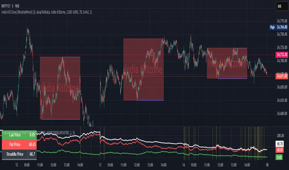
Straddle Charts - Live (Enhanced)Track options straddles with ease using the Straddle Charts - Live (Enhanced) indicator! Originally inspired by @mudraminer, this Pine Script v5 tool visualizes live call, put, and straddle prices for instruments like BANKNIFTY. Plotting call (green), put (red), and straddle (black) prices in a separate pane, it offers real-time insights for straddle strategy traders.
Key Features:
Live Data: Fetches 1-minute (customizable) option prices with error handling for invalid symbols.
Price Table: Displays call, put, straddle prices, and percentage change in a top-left table.
Volatility Alerts: Highlights bars with straddle price changes above a user-defined threshold (default 5%) with a yellow background and concise % labels.
Robust Design: Prevents plot errors with na checks and provides clear error messages.
How to Use: Input your call/put option symbols (e.g., NSE:NIFTY250814C24700), set the timeframe, and adjust the volatility threshold. Monitor straddle costs and volatility for informed trading decisions.
Perfect for options traders seeking a simple, reliable tool to track straddle performance. Check it out and share your feedback!
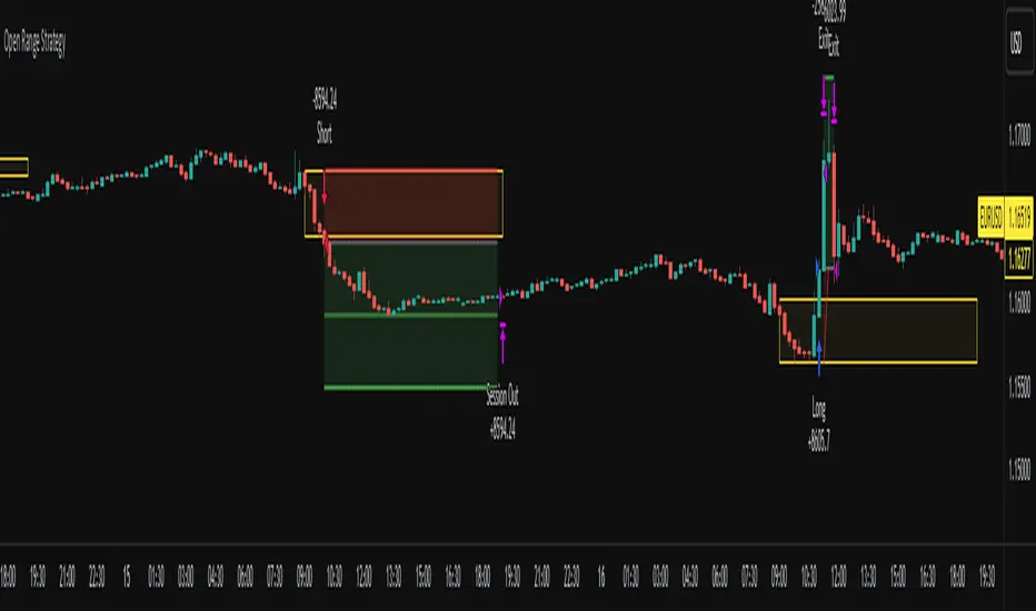
Open Range Breakout Strategy With Multi TakeProfitHello everyone,
For a while, I’ve been wanting to develop new scripts, but I couldn’t decide what to create. Eventually, I came up with the idea of coding traditional and well-known trading strategies—while adding modern features such as multi–take profit options. For the first strategy in this series, I chose the Open Range Strategy .
For those unfamiliar with it, the Open Range Strategy is a trading approach where you define a specific time period at the beginning of a trading session—such as the first 15 minutes, 30 minutes, or 1 hour—and mark the highest and lowest prices within that range. These levels then act as reference points for potential breakouts: if the price breaks above the range, it may signal a long entry; if it breaks below, it may indicate a short entry. This method is popular among day traders for capturing early momentum in the market.
Since this strategy is generally used as an intraday strategy , I added a Trade Session feature. This allows you to define the exact time window during which trades can be opened. Once the session ends, all positions are automatically closed, ensuring trades remain within your chosen intraday period.
Even though it’s a relatively simple concept, I’ve come across many different variations of it. That’s why I created a highly customizable project. Under the Session Settings, you can select the time window you want to define as your range. Whether it’s the first 15-minute candle or the entire first hour, the choice is entirely yours.
For stop-loss placement, there are two different options:
Middle of the Range – The stop loss is placed at the midpoint between the high and low of the defined range, offering a balanced buffer for both bullish and bearish setups.
Top/Bottom of the Range – The stop loss is placed just beyond the range’s high for short trades or just below the range’s low for long trades, providing a more conservative risk approach.
I’ve always been a big fan of the multi take-profit feature, so I added two different take-profit targets to this project. Take profits are calculated based on a Risk-to-Reward Ratio, which you can adjust in the settings. You can also set different position sizes for each target, allowing you to scale out of trades in a way that suits your strategy.
The result is a flexible, user-friendly strategy script that brings together a classic approach with modern risk management tools—ready to be tailored to your trading style
Backtest - Strategy Builder [AlgoAlpha]🟠 OVERVIEW
This script by AlgoAlpha is a modular Strategy Builder designed to let traders test custom trade entry and exit logic on TradingView without writing their own Pine code. It acts as a framework where users can connect multiple external signals, chain them in sequences, and run backtests with built-in leverage, margin, and risk controls. Its main strength is flexibility—you can define up to five sequential steps for entry and exit conditions on both long and short sides, with logic connectors (AND/OR) controlling how conditions combine. This lets you test complex multi-step confirmation workflows in a controlled, visual backtesting environment.
🟠 CONCEPTS
The system works by linking external signals —these can be values from other indicators, and/or custom sources—to conditional checks like “greater than,” “less than,” or “crossover.” You can stack these checks into steps , where all conditions in a step must pass before the sequence moves to the next. This creates a chain of logic that must be completed before a trade triggers. On execution, the strategy sizes positions according to your chosen leverage mode ( Cross or Isolated ) and allocation method ( Percent of equity or absolute USD value]). Liquidation prices are simulated for both modes, allowing realistic margin behaviour in testing. The script also tracks performance metrics like Sharpe, Sortino, profit factor, drawdown, and win rate in real time.
🟠 FEATURES
Up to 5 sequential steps for both long and short entries, each with multiple conditions linked by AND/OR logic.
Two leverage modes ( Cross and Isolated ) with independent long/short leverage multipliers.
Separate multi-step exit triggers for longs and shorts, with optional TP/SL levels or opposite-side triggers for flipping positions.
Position sizing by equity percent or fixed USD amount, applied before leverage.
Realistic liquidation price simulation for margin testing.
Built-in trade gating and validation—prevents trades if configuration rules aren’t met (e.g., no exit defined for an active side).
Full performance dashboard table showing live strategy status, warnings, and metrics.
Configurable bar coloring based on position side and TP/SL level drawing on chart.
Integration with TradingView's strategy backtester, allowing users to view more detailed metrics and test the strategy over custom time horizons.
🟠 USAGE
Add the strategy to your chart. In the settings, under Master Settings , enable longs/shorts, select leverage mode, set leverage multipliers, and define position sizing. Then, configure your Long Trigger and Short Trigger groups: turn on conditions, pick which external signal they reference, choose the comparison type, and assign them to a sequence step. For exits, use the corresponding Exit Long Trigger and Exit Short Trigger groups, with the option to link exits to opposite-side entries for auto-flips. You can also enable TP and/or SL exits with custom sources for the TP/SL levels. Once set, the strategy will simulate trades, show performance stats in the on-chart table, and highlight any configuration issues before execution. This makes it suitable for testing both simple single-signal systems and complex, multi-filtered strategies under realistic leverage and margin constraints.
🟠 EXAMPLE
The backtester on its own does not contain any indicator calculation; it requires input from external indicators to function. In this example, we'll be using AlgoAlpha's Smart Signals Assistant indicator to demonstrate how to build a strategy using this script.
We first define the conditions beforehand:
Entry :
Longs – SSA Bullish signal (strong OR weak)
Shorts – SSA Bearish signal (strong OR weak)
Exit
Longs/Shorts: (TP/SL hit OR opposing signal fires)
Other Parameters (⚠️Example only, tune this based on proper risk management and settings)
Long Leverage: default (3x)
Short Leverage: default (3x)
Position Size: default (10% of equity)
Steps
Load up the required indicators (in this example, the Smart Signals Assistant).
Ensure the required plots are being output by the indicator properly (signals and TP/SL levels are being plotted).
Open the Strategy Builder settings and scroll down to "CONDITION SETUP"; input the signals from the external indicator.
Configure the exit conditions, add in the TP/SL levels from the external indicator, and add an additional exit condition → {{Opposite Direction}} Entry Trigger.
After configuring the entry and exit conditions, the strategy should now be running. You can view information on the strategy in TradingView's backtesting report and also in the Strategy Builder's information table (default top right corner).
It is important to note that the strategy provided above is just an example, and the complexity of possible strategies stretches beyond what was shown in this short demonstration. Always incorporate proper risk management and ensure thorough testing before trading with live capital.
Ücretli komut dosyası

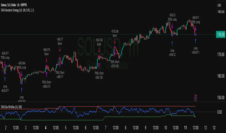
EMA Deviation Strategy📌 Strategy: EMA Deviation Strategy
The EMA Deviation Strategy identifies potential reversal points by measuring how far the current price deviates from its Exponential Moving Average (EMA). It dynamically tracks the minimum and maximum deviation levels over a user-defined lookback period, and enters trades when price reaches extreme zones.
🔍 Core Logic:
• Buy Entry: When price deviates significantly below the EMA, approaching the historical minimum deviation — signaling a potential rebound.
• Sell Entry: When price deviates significantly above the EMA, nearing the historical maximum deviation — signaling a possible pullback.
• Optional Take Profit / Stop Loss: Manage risk with customizable exit levels.
⚙️ Customizable Inputs:
• EMA length and lookback period
• Threshold sensitivity for entry signals
• Take profit and stop loss percentages
📈 Best Used For:
• Mean reversion setups
• Assets with cyclical or range-bound behavior
• Identifying short-term overbought/oversold conditions
Mutanabby_AI | Algo Pro Strategy# Mutanabby_AI | Algo Pro Strategy: Advanced Candlestick Pattern Trading System
## Strategy Overview
The Mutanabby_AI Algo Pro Strategy represents a systematic approach to automated trading based on advanced candlestick pattern recognition and multi-layered technical filtering. This strategy transforms traditional engulfing pattern analysis into a comprehensive trading system with sophisticated risk management and flexible position sizing capabilities.
The strategy operates on a long-only basis, entering positions when bullish engulfing patterns meet specific technical criteria and exiting when bearish engulfing patterns indicate potential trend reversals. The system incorporates multiple confirmation layers to enhance signal reliability while providing comprehensive customization options for different trading approaches and risk management preferences.
## Core Algorithm Architecture
The strategy foundation relies on bullish and bearish engulfing candlestick pattern recognition enhanced through technical analysis filtering mechanisms. Entry signals require simultaneous satisfaction of four distinct criteria: confirmed bullish engulfing pattern formation, candle stability analysis indicating decisive price action, RSI momentum confirmation below specified thresholds, and price decline verification over adjustable lookback periods.
The candle stability index measures the ratio between candlestick body size and total range including wicks, ensuring only well-formed patterns with clear directional conviction generate trading signals. This filtering mechanism eliminates indecisive market conditions where pattern reliability diminishes significantly.
RSI integration provides momentum confirmation by requiring oversold conditions before entry signal generation, ensuring alignment between pattern formation and underlying momentum characteristics. The RSI threshold remains fully adjustable to accommodate different market conditions and volatility environments.
Price decline verification examines whether current prices have decreased over a specified period, confirming that bullish engulfing patterns occur after meaningful downward movement rather than during sideways consolidation phases. This requirement enhances the probability of successful reversal pattern completion.
## Advanced Position Management System
The strategy incorporates dual position sizing methodologies to accommodate different account sizes and risk management approaches. Percentage-based position sizing calculates trade quantities as equity percentages, enabling consistent risk exposure across varying account balances and market conditions. This approach proves particularly valuable for systematic trading approaches and portfolio management applications.
Fixed quantity sizing provides precise control over trade sizes independent of account equity fluctuations, offering predictable position management for specific trading strategies or when implementing precise risk allocation models. The system enables seamless switching between sizing methods through simple configuration adjustments.
Position quantity calculations integrate seamlessly with TradingView's strategy testing framework, ensuring accurate backtesting results and realistic performance evaluation across different market conditions and time periods. The implementation maintains consistency between historical testing and live trading applications.
## Comprehensive Risk Management Framework
The strategy features dual stop loss methodologies addressing different risk management philosophies and market analysis approaches. Entry price-based stop losses calculate stop levels as fixed percentages below entry prices, providing predictable risk exposure and consistent risk-reward ratio maintenance across all trades.
The percentage-based stop loss system enables precise risk control by limiting maximum loss per trade to predetermined levels regardless of market volatility or entry timing. This approach proves essential for systematic trading strategies requiring consistent risk parameters and capital preservation during adverse market conditions.
Lowest low-based stop losses identify recent price support levels by analyzing minimum prices over adjustable lookback periods, placing stops below these technical levels with additional buffer percentages. This methodology aligns stop placement with market structure rather than arbitrary percentage calculations, potentially improving stop loss effectiveness during normal market fluctuations.
The lookback period adjustment enables optimization for different timeframes and market characteristics, with shorter periods providing tighter stops for active trading and longer periods offering broader stops suitable for position trading approaches. Buffer percentage additions ensure stops remain below obvious support levels where other market participants might place similar orders.
## Visual Customization and Interface Design
The strategy provides comprehensive visual customization through eight predefined color schemes designed for different chart backgrounds and personal preferences. Color scheme options include Classic bright green and red combinations, Ocean themes featuring blue and orange contrasts, Sunset combinations using gold and crimson, and Neon schemes providing high visibility through bright color selections.
Professional color schemes such as Forest, Royal, and Fire themes offer sophisticated alternatives suitable for business presentations and professional trading environments. The Custom color scheme enables precise color selection through individual color picker controls, maintaining maximum flexibility for specific visual requirements.
Label styling options accommodate different chart analysis preferences through text bubble, triangle, and arrow display formats. Size adjustments range from tiny through huge settings, ensuring appropriate visual scaling across different screen resolutions and chart configurations. Text color customization maintains readability across various chart themes and background selections.
## Signal Quality Enhancement Features
The strategy incorporates signal filtering mechanisms designed to eliminate repetitive signal generation during choppy market conditions. The disable repeating signals option prevents consecutive identical signals until opposing conditions occur, reducing overtrading during consolidation phases and improving overall signal quality.
Signal confirmation requirements ensure all technical criteria align before trade execution, reducing false signal occurrence while maintaining reasonable trading frequency for active strategies. The multi-layered approach balances signal quality against opportunity frequency through adjustable parameter optimization.
Entry and exit visualization provides clear trade identification through customizable labels positioned at relevant price levels. Stop loss visualization displays active risk levels through colored line plots, ensuring complete transparency regarding current risk management parameters during live trading operations.
## Implementation Guidelines and Optimization
The strategy performs effectively across multiple timeframes with optimal results typically occurring on intermediate timeframes ranging from fifteen minutes through four hours. Higher timeframes provide more reliable pattern formation and reduced false signal occurrence, while lower timeframes increase trading frequency at the expense of some signal reliability.
Parameter optimization should focus on RSI threshold adjustments based on market volatility characteristics and candlestick pattern timeframe analysis. Higher RSI thresholds generate fewer but potentially higher quality signals, while lower thresholds increase signal frequency with corresponding reliability considerations.
Stop loss method selection depends on trading style preferences and market analysis philosophy. Entry price-based stops suit systematic approaches requiring consistent risk parameters, while lowest low-based stops align with technical analysis methodologies emphasizing market structure recognition.
## Performance Considerations and Risk Disclosure
The strategy operates exclusively on long positions, making it unsuitable for bear market conditions or extended downtrend periods. Users should consider market environment analysis and broader trend assessment before implementing the strategy during adverse market conditions.
Candlestick pattern reliability varies significantly across different market conditions, with higher reliability typically occurring during trending markets compared to ranging or volatile conditions. Strategy performance may deteriorate during periods of reduced pattern effectiveness or increased market noise.
Risk management through stop loss implementation remains essential for capital preservation during adverse market movements. The strategy does not guarantee profitable outcomes and requires proper position sizing and risk management to prevent significant capital loss during unfavorable trading periods.
## Technical Specifications
The strategy utilizes standard TradingView Pine Script functions ensuring compatibility across all supported instruments and timeframes. Default configuration employs 14-period RSI calculations, adjustable candle stability thresholds, and customizable price decline verification periods optimized for general market conditions.
Initial capital settings default to $10,000 with percentage-based equity allocation, though users can adjust these parameters based on account size and risk tolerance requirements. The strategy maintains detailed trade logs and performance metrics through TradingView's integrated backtesting framework.
Alert integration enables real-time notification of entry and exit signals, stop loss executions, and other significant trading events. The comprehensive alert system supports automated trading applications and manual trade management approaches through detailed signal information provision.
## Conclusion
The Mutanabby_AI Algo Pro Strategy provides a systematic framework for candlestick pattern trading with comprehensive risk management and position sizing flexibility. The strategy's strength lies in its multi-layered confirmation approach and sophisticated customization options, enabling adaptation to various trading styles and market conditions.
Successful implementation requires understanding of candlestick pattern analysis principles and appropriate parameter optimization for specific market characteristics. The strategy serves traders seeking automated execution of proven technical analysis techniques while maintaining comprehensive control over risk management and position sizing methodologies.

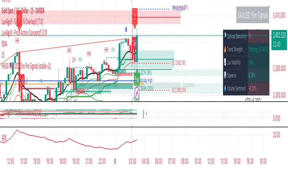
Hassi XAUUSD STRATEGY BOTGold (XAUUSD) 15m trend+momentum based signals with EMA(9/21/200), RSI, custom ADX, ATR-based SL/TP & alerts
Works on XAUUSD 15m.
Entry: EMA9/21 cross + price relative to EMA200 + RSI filter + custom ADX trend strength.
Risk: default SL=1.5×ATR, TP=2×ATR (editable).
Notes: No financial advice. Backtest before live use. Avoid high-impact news whipsaws.
Backtest [OptAlgo]This backtest script is designed to convert ideas or indicators into backtest results. The script creates buy/sell signals by comparing price sources against fixed values or other imported plots using many comparison methods. It has many features including multiple exit systems: TP/SL, custom plot-based stops and more. It supports full trading automation through webhook alerts with live signal processing.
🔢 Signal Creation System
→ Values Group : Compare price sources against fixed numerical values
→ Plots Group : Compare two different price sources/indicators against each other
→ Flexible Comparisons : 15+ comparison methods (equal, crossover, rising...)
→ Signal Types : Long, Short, Close All, Block signals, and combination signals
→ Merge Rules : Minimum condition requirements for signal activation
🔀 Advanced Signal Logic
→ Counter Signals : Choose between reversing positions or closing them
→ Signal Inversion : Flip all buy/sell signals with one toggle
→ External Signal Import : Import coded signals (1=Long, -1=Short, 0=Close)
→ Day Blocker : Enable/disable trading on specific weekdays
→ Session Control : Limit trading to specific market sessions
⚙️ Strategy Settings
→ Position Sides : All Ways, Long Only, or Short Only modes
→ Signal Control : Individual enable/disable for long and short signals
→ Counter Signal Mode : Reverse Open Position vs Close Open Position
→ Signal Reversal : Global signal inversion capability
🔰 Risk Management (Limiter Settings)
→ Leverage Control : Leverage with liquidation warnings
→ Drawdown Limit : Auto-halt strategy at specified drawdown percentage
→ Tradable Ratio : Use portion of available balance (0.01-1.0)
→ Contract Limit : Cap maximum contract size regardless of balance
🎯 TP/SL System
→ Fixed TP/SL : Set percentage-based take profit and stop loss
→ Custom Plot Stops : Use any indicator/plot as dynamic stop loss
→ ATR-Based Exits : Volatility-adjusted TP/SL using Average True Range
→ Realistic Protection : Prevents unrealistic TP/SL prices in live trading
→ Stop Modes : Instant (Sudden) vs Candle Close execution
→ ATR Stop Loss : Override fixed SL with volatility-based calculations
→ ATR Take Profit : Dynamic TP based on market volatility
→ Trailing Options : Safe, Normal, or Aggressive trailing methods
→ Calculation Modes : Normal, Volume-weighted, or Limited (with max %) options
→ Volume Integration : ATR levels adjust based on volume influx
🤖 Automation & Alerts
→ Webhook Integration : Send JSON alerts for automated execution
→ Live Signals : Real-time signal processing (every tick vs bar close)
→ Strategy Key : Unique identifier for automated systems
→ Early Entry : Send alerts X seconds before candle close
→ Fast Execution : Prevent signal lag in automated trading
🐞 Development Tools
→ Alert Plotting : Visualize signals directly on chart (disable for live alerts)
→ Professional Mode : Remove UI controls for faster calculation
→ Debug : Metrics are plotted in data window.
📊 Key Advantages
→ Multi-Condition Logic : Combine multiple indicators with flexible rules
→ Risk-First Design : Built-in drawdown and leverage protection
→ Automation Ready : Full webhook and alert system integration
⚠️ Important Warnings
→ High leverage combined with high SL may adjust to liquidation price
→ Use consistent leverage across all strategies on same trading isolated margin pair
→ Live signals require "Calculate on every tick" enabled in settings
→ Disable alert plotting when creating actual alerts to prevent latency

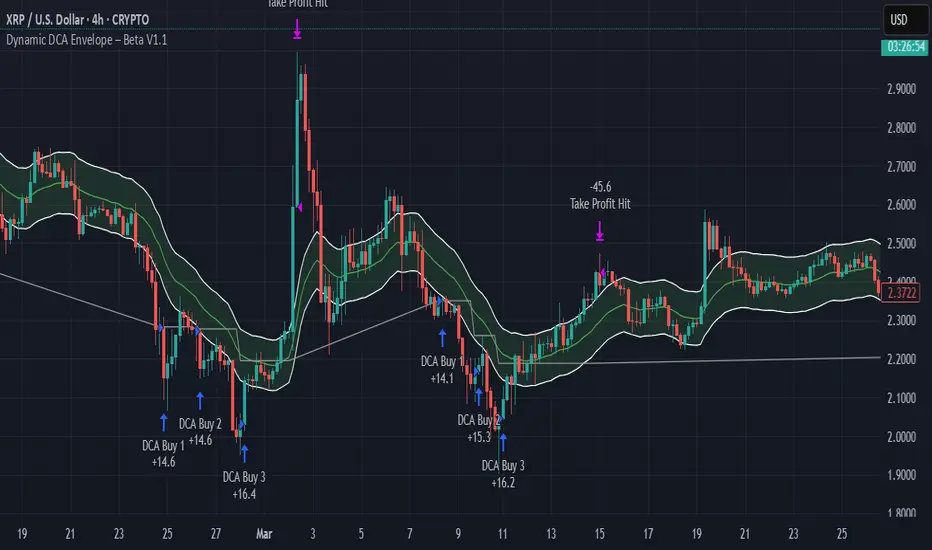
Dynamic DCA Envelope – Beta V1.1Dynamic DCA Envelope-Beta V1.1 is a preview version of a Dollar-Cost Averaging (DCA) strategy designed for trending or volatile markets.
-Long Positions Only
-Intended for Cryptocurrency, but can be used in any market
-1 and 4 hour timeframe
-Average Commissions 0.1%-0.3% per trade (Cryptocurrency)
What it does:
This strategy identifies buying opportunities when price closes below a dynamic envelope (based on EMA). After 3 consecutive closes below the lower envelope, the system arms a buy condition. A DCA buy-in is triggered when price bounces by a configurable percentage from the trailing low. The strategy supports up to 3 buy-ins, each equally sized, and closes the entire position at a fixed take profit or stop loss.
How it works:
-Entry logic is based on price deviation from an EMA envelope
-Waits for 3 closes below the envelope to detect weakness
-Uses bounce percentage from the lowest point to trigger each buy
-Includes cooldown logic between buys to avoid clustering
-All positions are closed when TP or SL is hit
How to use it:
-Use on trending assets with volatility (e.g., crypto, tech stocks)
-Adjust inputs to match asset behavior:
-EMA Length
-Envelope Offset %
-Bounce % (Trailing DCA)
-Take Profit / Stop Loss
-View strategy performance in the Strategy Tester tab
What’s unique:
Unlike most DCA scripts that immediately average down, this version includes:
-Trigger logic requiring multiple closes below trend
-Bounce-based entry to avoid catching a falling knife
-Cooldown resets to prevent overtrading
-A true entry–wait–buy–reset loop mimicking disciplined execution
*This is a beta version intended as a preview. A full Pro version is in development, which includes:
-SmartScaling logic
-Trailing take profit
-Multi-symbol scanning
-Backtest range limits
-Risk-adjusted filtering
SAFE Leverage x50Description:
Safe Leverage x50 is an indicator designed to help traders choose prudent, realistic, and dynamic leverage, adapted to the timeframe and volatility of the asset they are trading.
Based on rigorous statistical and practical observation, this indicator does not propose fixed rules, but rather provides a visual estimate of the maximum leverage a typical trade can tolerate without being liquidated, based on the current candle's movement range. At the same time, it automatically suggests a more conservative leverage (by default, half of the maximum) for more controlled risk management.

SwingTrade ADX Strategy v6This is a swing trading strategy that combines VWAP (Volume Weighted Average Price), ADX (Average Directional Index) for trend strength, and volume ratios to generate long/short entry and exit signals. It's designed for daily charts but can be adapted.
#### Key Features:
- **Entries**: Based on VWAP crossovers, rising/falling delta (price deviation from VWAP), ADX trend confirmation, and volume ratios.
- **Exits**: Dynamic exits when VWAP delta reverses after a peak.
- **Filters**: Optional toggles for VWAP signals, ADX, and volume. Backtest date range for custom periods.
- **Visuals**: VWAP line, signal shapes/labels, and an info panel showing key metrics (VWAP Delta %, ADX, Volume Ratio).
- **Alerts**: Built-in alerts for buy/sell entries and exits.
#### How to Use:
1. Apply to your chart (e.g., stocks, forex, crypto).
2. Adjust parameters in the settings (e.g., ADX threshold, volume period).
3. Enable/disable indicators as needed.
4. Backtest using the date filters and review equity curve.
**Disclaimer**: This is for educational purposes only. Past performance is not indicative of future results. Not financial advice—trade at your own risk. Backtest thoroughly and use with proper risk management.
Feedback welcome! If you find it useful, give it a like.

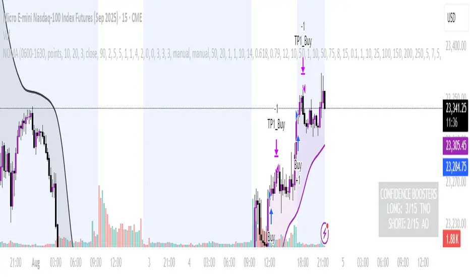
NOMANOMA Adaptive Confidence Strategy —
What is NOMA?
NOMA is a next-generation, confidence-weighted trading strategy that fuses modern trend logic, multi-factor market structure, and adaptive risk controls—delivering a systematic edge across futures, stocks, forex, and crypto markets. Designed for precision, adaptability, and hands-off automation, NOMA provides actionable trade signals and real-time alerts so you never miss a high-conviction opportunity.
Key Benefits & Why Use NOMA?
Trade With Confidence, Not Guesswork:
NOMA combines over 11 institutional-grade confirmations (market structure, order flow, volatility, liquidity, SMC/ICT concepts, and more) into a single “confidence score” engine. Every trade entry is filtered through customizable booster weights, so only the strongest opportunities trigger.
Built-In Alerts:
Get instant notifications on all entries, take-profits, trailing stop events, and exits. Connect alerts to your mobile, email, or webhook for seamless automation or just peace of mind.
Advanced Position Management:
Supports up to 5 separate take-profit levels with adjustable quantities, plus dynamic and stepwise trailing stops. Protects your gains and adapts exit logic to market movement, not just static targets.
Anti-Chop/No Trade Zones:
Eliminate low-probability, sideways market conditions using the “No Chop Zone” filter, so you only trade in meaningful, trending environments.
Full Market Session Control:
Restrict trades to custom sessions (e.g., New York hours) for added discipline and to avoid overnight risk.
— Ideal for day traders and prop-firm requirements.
Multi-Asset & Timeframe Support:
Whether you trade micro futures, stocks, forex, or crypto, NOMA adapts its TP/SL logic to ticks, pips, or points and works on any timeframe.
How NOMA Works (Feature Breakdown)
1. Adaptive Trend Engine
Uses a custom NOMA line that blends classic moving averages with dynamic momentum and a proprietary “Confidence Momentum Oscillator” overlay.
Visual trend overlay and color fill for easy chart reading.
2. Multi-Factor Confidence Scoring
Each trade is scored on up to 11 confidence “boosters,” including:
Market Manipulation & Accumulation (detects smart money traps and true range expansions)
Accumulation/Distribution (AD line)
ATR Volatility Rank (prioritizes trades when volatility is “just right”)
COG Cross (center of gravity reversal points)
Change of Character/Break of Structure (CHoCH/BOS logic, SMC/ICT style)
Order Blocks, Breakers, FVGs, Inducements, OTE (Optimal Trade Entry) Zones
You control the minimum score required for a trade to trigger, plus the weight of each factor (customize for your asset or style).
3. Smart Trade Management
Step Take-Profits:
Up to 5 profit targets, each with individual contract/quantity splits.
Step Trailing Stop:
Trail your stop with a ratcheting logic that tightens after each TP is hit, or use a fully dynamic ATR-based trail for volatile markets.
Kill-Switch:
Instant trailing stop logic closes all open contracts if price reverses sharply.
4. Session Filter & Cooldown Logic
Restricts trading to key sessions (e.g., NY open) to avoid low-liquidity or dead zones.
Cooldown bars prevent “overtrading” or rapid re-entries after an exit.
5. Chop Zone Filter
Optionally blocks trades during flat/choppy periods using a custom “NOMA spread” calculation.
When enabled, background color highlights no-trade periods for clarity.
6. Real-Time Alerts
Receive alerts for:
Trade entries (long & short, with confidence score)
Every take-profit target hit
Trailing stop exits or full position closes
Easy setup: Create alerts for all conditions and get notified instantly.
Customization & Inputs
TP/SL Modes: Choose between manual, ATR-multiplied, or hybrid take-profit and trailing logic.
Position Sizing: Fixed contracts/quantity per trade, with customizable splits for scaling out.
Session Settings: Restrict to any time window.
Confidence Engine: User-controlled weights and minimum score—tailor for your asset.
Risk & Volatility Filters: ATR length/multiplier, min/max range, and more.
How To Use
Add NOMA to your chart.
Customize your settings (session, TPs, confidence scores, etc.).
Set up TradingView alerts (“Any Alert() function call”) to receive notifications.
Monitor trade entries, profit targets, and stops directly on your chart or in your inbox.
Adjust confidence weights as you optimize for your favorite asset.
Pro Tips
Start with default settings—they are optimized for NQ micro futures, 15m timeframe.
Increase the minimum confidence score or weights for stricter filtering in volatile or low-liquidity markets.
Adjust your take-profit and trailing stop settings to match your trading style (scalping vs. swing).
Enable “No Chop Zone” during sideways conditions for cleaner signals.
Test in strategy mode before trading live to dial in your risk and settings.
Disclaimer
This script is for educational and research purposes only. No trading system guarantees future results.
Performance will vary by symbol, timeframe, and market regime—always test settings and use at your own risk. Not investment advice.
If alerts or strategy entries are not triggering as expected, try lowering the minimum confidence score or disabling certain boosters.
This will come with a user manual please do not hesitate to message me to gain access. TO THE MOON AND BEYOND
PHANTOM STRIKE Z-4 [ApexLegion]Phantom Strike Z-4
STRATEGY OVERVIEW
This strategy represents an analytical framework using 6 detection systems that analyze distinct market dimensions through adaptive timeframe optimization. Each system targets specific market inefficiencies - automated parameter adjustment, market condition filtering, phantom strike pattern detection, SR exit management, order block identification, and volatility-aware risk management - with results processed through a multi-component scoring calculation that determines signal generation and position management decisions.
SYSTEM ARCHITECTURE PHILOSOPHY
Phantom Strike Z-4 operates through 12 distinct parameter groups encompassing individual settings that allow detailed customization for different trading environments. The strategy employs modular design principles where each analytical component functions independently while contributing to unified decision-making protocols. This architecture enables traders to engage with structured market analysis through intuitive configuration options while the underlying algorithms handle complex computational processes.
The framework approaches certain aspects differently from static trading approaches by implementing real-time parameter adjustment based on timeframe characteristics, market volatility conditions, news event detection, and weekend gap analysis. During low-volatility periods where traditional strategies struggle to generate meaningful returns, Z-4's adaptive systems identify micro-opportunities through formation analysis and systematic patience protocols.
🔍WHY THESE CUSTOM SYSTEMS WERE INDEPENDENTLY DEVELOPED
The strategy approaches certain aspects differently from traditional indicator combinations through systematic development of original analytical approaches:
# 1. Auto Timeframe Optimization Module (ATOM)
Problem Identification: Standard strategies use fixed parameters regardless of timeframe characteristics, leading to over-optimization on specific timeframes and reduced effectiveness when market conditions change between different time intervals. Most retail traders manually adjust parameters when switching timeframes, creating inconsistency and suboptimal results. Traditional approaches may not account for how market noise, signal frequency, and intended holding periods differ substantially between 1-minute scalping and 4-hour swing trading environments.
Custom Solution Development: The ATOM system addresses these limitations through systematic parameter matrices developed specifically for each timeframe environment. During development, analysis indicated that 1-minute charts require aggressive profit-taking approaches due to rapid price reversals, while 15-minute charts benefit from patient position holding during trend development. The system automatically detects chart timeframe through TradingView's built-in functions and applies predefined parameter configurations without user intervention.
Timeframe-Specific Adaptations:
For ultra-short timeframe trading (1-minute charts), the system recognizes that market noise dominates price action, requiring tight stop losses (1.0%) and rapid profit realization (25% at TP1, 35% at TP2, 40% at TP3). Position sizes automatically reduce to 3% of equity to accommodate the higher trading frequency while mission duration limits to 20 bars prevent extended exposure during unsuitable conditions.
Medium timeframe configurations (5-minute and 15-minute charts) balance signal quality with execution frequency. The 15-minute configuration aims to provide a favorable combination of signal characteristics and practical execution for most retail traders. Formation thresholds increase to 2.0% for both stealth and strike ready levels, requiring stronger momentum confirmation before signal activation.
Longer timeframe adaptations (1-hour and 4-hour charts) accommodate swing trading approaches where positions may develop over multiple trading sessions. Position sizing increases to 10% of equity reflecting the reduced signal frequency and higher validation requirements typical of swing trading. Take profit targets extend considerably (TP1: 2.0%, TP2: 4.0%, TP3: 8.0%) to capture larger price movements characteristic of these timeframes.
# 2. Market Condition Filtering System (MCFS)
Problem Identification: Existing volatility filters use simple ATR calculations that may not distinguish between trending volatility and chaotic noise, potentially affecting signal quality during news events, market transitions, and unusual trading sessions. Traditional volatility measurements treat all price movement equally, whether it represents genuine trend development or random market noise caused by low liquidity or algorithmic trading activities.
Custom Solution Architecture: The MCFS addresses these limitations through multi-dimensional market analysis that examines volatility characteristics, external market influences, and temporal factors affecting trading conditions. Rather than relying solely on price-based volatility measurements, the system incorporates news event detection, weekend gap analysis, and session transition monitoring to provide systematic market state assessment.
Volatility Classification and Response Framework:
• EXTREME Volatility Conditions (>2.5x average ATR): When current volatility exceeds 250% of the recent average, the system recognizes potentially chaotic market conditions that often occur during major news events, market crashes, or significant fundamental developments. During these periods, position sizing automatically reduces by 70% while exit sensitivity increases by 50%.
• HIGH Volatility Conditions (1.8-2.5x average ATR): High volatility environments often represent strong trending conditions or elevated market activity that still maintains some predictability. Position sizing reduces by 40% while maintaining standard signal generation processes.
• NORMAL Volatility Conditions (1.2-1.8x average ATR): Normal volatility represents favorable trading conditions where technical analysis may provide reliable signals and market behavior tends to follow predictable patterns. All strategy parameters operate at standard settings.
• LOW Volatility Conditions (0.8-1.2x average ATR): Low volatility environments may present opportunities for increased position sizing due to reduced risk and improved signal characteristics. Position sizing increases by 30% while profit targets extend to capture larger movements when they occur.
• DEAD Volatility Conditions (<0.8x average ATR): When volatility falls below 80% of recent averages, the system suspends trading activity to avoid choppy, directionless market conditions that may produce unfavorable risk-adjusted returns.
# 3. Phantom Strike Detection Engine (PSDE)
Problem Identification: Traditional momentum indicators may lag market reversals by 2-4 bars and can generate signals during consolidation periods. Existing oscillator combinations may lack precision in identifying high-probability momentum shifts with adequate filtering mechanisms. Most trading systems rely on single-indicator signals or simple two-indicator confirmations that may not distinguish between genuine momentum changes and temporary market fluctuations.
Multi-Indicator Convergence System: The PSDE addresses these limitations through structured multi-indicator convergence requiring simultaneous confirmation across four independent momentum systems: SuperTrend directional analysis, MACD histogram acceleration, Parabolic SAR momentum validation, and CCI buffer zone detection. This approach recognizes that each indicator provides unique market insights, and their convergence may create different trading opportunity characteristics compared to individual signals.
Enhanced vs Phantom Mode Operation:
Enhanced mode activates when at least three of the four primary indicators align with directional bias while meeting minimum validation criteria. Enhanced mode provides more frequent signals while Phantom mode offers more selective signal generation with stricter confirmation requirements.
Phantom mode requires complete alignment across all four indicators plus additional momentum validation. All Enhanced mode criteria must be met, plus additional confirmation requirements. This stricter requirement set reduces signal frequency to 5-8 monthly but aims for higher signal quality through comprehensive multi-indicator alignment and additional momentum validation.
# 4. Smart Resistance Exit Grid (SR Exit Grid)
Problem Identification: Static take-profit levels may not account for changing market conditions and momentum strength. Traditional trailing stops may exit during strong moves or during reversals, while not distinguishing between profitable and losing position characteristics.
Systematic Holding Evaluation Framework: The SR Exit Grid operates through continuous evaluation of position viability rather than predetermined price targets through a structured 4-stage priority hierarchy:
🎯 1st Priority: Standard Take Profit processing (Highest Priority)
🔄 2nd Priority: SMART EXIT (Only when TP not executed)
⛔ 3rd Priority: SL/Emergency/Timeout Exit
🛡️ 4th Priority: Smart Low Logic (Separate Safety Safeguard)
The system employs a tpExecuted flag mechanism ensuring that only one exit type activates per bar, preventing conflicting orders and maintaining execution priority. Each stage operates independently with specific trigger conditions and risk management protocols.
Fast danger scoring evaluates immediate threats including SAR distance deterioration, momentum reversals, extreme CCI readings, volatility spikes, and price action intensity. When combined scores exceed specified thresholds (8.0+ danger with <2.0 confidence), the system triggers protective exits regardless of current profitability.
# 5. Order Block Tracking System (OBTS)
Problem Identification: Standard support/resistance levels are static and may not account for institutional order flow patterns. Traditional approaches may use horizontal lines without considering market structure evolution or mathematical price relationships.
Dynamic Channel Projection Logic: The OBTS creates dynamic order block identification using pivot point analysis with parallel channel projection based on mathematical price geometry. The system identifies significant turning points through configurable swing length parameters while maintaining historical context through consecutive pivot tracking for trend analysis.
Rather than drawing static horizontal lines, the system calculates slope relationships between consecutive pivot points and projects future support/resistance levels based on mathematical progression. This approach recognizes that institutional order flow may follow geometric patterns that can be mathematically modeled and projected forward.
# 6. Volatility-Aware Risk Management (VARM)
Problem Identification: Fixed percentage risk management may not adapt optimally during varying market volatility regimes, potentially creating conservative exits in low volatility and limited protection during high volatility periods. Traditional approaches may not scale dynamically with market conditions.
Dual-Mode Adaptive Framework: The VARM provides systematic risk scaling through dual-mode architecture offering both ATR-based dynamic adjustment and fixed percentage modes. Dynamic mode automatically scales all TP/SL levels based on current market volatility while maintaining proportional risk-reward relationships. Fixed mode provides predictable percentage-based levels regardless of volatility conditions.
Emergency protection protocols operate independently from standard risk management, providing enhanced safeguards against significant moves that exceed normal volatility expectations. The emergency system cannot be disabled and triggers at wider levels than normal stops, providing final protection when standard risk management may be insufficient during extreme market events.
## Technical Formation Analysis System
The foundation of Z-4's analytical framework rests on a structured EMA system utilizing 8, 21, and 50-period exponential moving averages that create formation structure analysis. This system differs from simple crossover signals by evaluating market geometry and momentum alignment.
Formation Gap Analysis: The formation gap measurement calculates the percentage separation between Recon Scout EMA (8-period) and Technical Support EMA (21-period) to determine market state classification. When gap percentage falls below the Stealth Mode Threshold (default 1.5%), the market enters consolidation phase requiring enhanced patience. When gap exceeds Strike Ready Threshold (1.5%), conditions become favorable for momentum-based entries.
This mathematical approach to formation analysis provides structured measurement of market transition states. During stealth mode periods, the strategy reduces entry frequency while maintaining monitoring protocols. Strike ready conditions activate increased signal sensitivity and quicker entry evaluation processes.
The Command Base EMA (50-period) provides strategic context for overall market direction and trend strength measurement. Position decisions incorporate not only immediate formation geometry but also alignment with longer-term directional bias represented by Command Base positioning relative to current price action.
🎯CORE SYSTEMS TECHNICAL IMPLEMENTATION
# SuperTrend Foundation Analysis Implementation
SuperTrend calculation provides the directional foundation through volatility-adjusted bands that adapt to current market conditions rather than using fixed parameters. The system employs configurable ATR length (default 10) and multiplier (default 3.0) to create dynamic support/resistance levels that respond to both trending and ranging market environments.
Volatility-Adjusted Band Calculation:
st_atr = ta.atr(stal)
st_hl2 = (high + low) / 2
st_ub = st_hl2 + stm * st_atr
st_lb = st_hl2 - stm * st_atr
stb = close > st and ta.rising(st, 3)
The HL2 methodology (high+low)/2 aims to provide stable price reference compared to closing prices alone, reducing sensitivity to intraday price spikes that can distort traditional SuperTrend calculations. ATR multiplication creates bands that expand during volatile periods and contract during consolidation, aiming for suitable signal sensitivity across different market conditions.
Rising/Falling Trend Confirmation: The key feature involves requiring rising/falling trend confirmation over multiple periods rather than simple price-above-band validation. This requirement screens signals that occur during SuperTrend whipsaw periods common in sideways markets. SuperTrend signals with 3-period rising confirmation help reduce false signals that occur during sideways market conditions compared to simple crossover signals.
Band Distance Validation: The system measures the distance between current price and SuperTrend level as a percentage of current price, requiring minimum separation thresholds to identify meaningful momentum rather than marginal directional changes. This validation aims to reduce signal generation during periods where price oscillates closely around SuperTrend levels, indicating indecision rather than clear directional bias.
# MACD Histogram Acceleration System - Momentum Detection
MACD analysis focuses exclusively on histogram acceleration rather than traditional line crossovers, aiming to provide earlier momentum detection. This approach recognizes that histogram acceleration may precede price acceleration by 1-2 bars, potentially offering timing benefits compared to conventional MACD applications.
Acceleration-Based Signal Generation:
mf = ta.ema(close, mfl)
ms = ta.ema(close, msl)
ml = mf - ms
msg = ta.ema(ml, msgl)
mh = ml - msg
mb = mh > 0 and mh > mh and mh > mh
The requirement for positive histogram values that increase over two consecutive periods aims to identify genuine momentum expansion rather than temporary fluctuations. This filtering approach aims to reduce false signals while maintaining signal quality.
Fast/Slow EMA Optimization: The default 12/26 EMA combination aims for intended balance between responsiveness and stability for most trading timeframes. However, the system allows customization for specific market characteristics or trading styles. Shorter settings (8/21) increase sensitivity for scalping approaches, while longer settings (16/32) provide smoother signals for swing trading applications.
Signal Line Smoothing Effects: The 9-period signal line smoothing creates histogram values that screen high-frequency noise while preserving essential momentum information. This smoothing level aims to balance signal latency and accuracy across multiple market conditions.
# Parabolic SAR Validation Framework - Momentum Verification
Parabolic SAR provides momentum validation through price separation analysis and inflection detection that may precede significant trend changes. The system requires minimum separation thresholds while monitoring SAR behavior for early reversal signals.
Separation-Based Validation:
sar = ta.sar(ss, si, sm)
sarb = close > sar and (close - sar) / close > 0.005
sardp = math.abs(close - sar) / close * 100
sariu = sarm > 0 and sarm < 0 and math.abs(sarmc) > saris
The 0.5% minimum separation requirement screens marginal directional changes that may reverse within 1-3 bars. The 0.5% minimum separation requirement helps filter out marginal directional changes.
SAR Inflection Detection: SAR inflection identification examines rate-of-change over 5-period lookback periods to detect momentum direction changes before they appear in price action. Inflection sensitivity (default 1.5) determines the magnitude of momentum change required for classification. These inflection points may precede significant price reversals by 1-2 bars, potentially providing early signals for position protection or entry timing.
Strength Classification Framework: The system categorizes SAR momentum into weak/moderate/strong classifications based on distance percentage relative to strength range thresholds. Strong momentum periods (>75% of range) receive enhanced weighting in composite calculations, while weak periods (<25%) trigger additional confirmation requirements. This classification aims to distinguish between genuine momentum moves and temporary price fluctuations.
# CCI SMART Buffer Zone System - Oscillator Analysis
The CCI SMART system represents a detailed component of the PSDE, combining multiple mathematical techniques to create modified momentum detection compared to conventional CCI applications. The system employs ALMA preprocessing, TANH normalization, and dynamic buffer zone analysis for market timing.
ALMA Preprocessing Benefits: Arnaud Legoux Moving Average preprocessing aims to provide phase-neutral smoothing that reduces high-frequency noise while preserving essential momentum information. The configurable offset (0.85) and sigma (6.0) parameters create Gaussian filter characteristics that aim to maintain signal timing while reducing unwanted signals caused by random price fluctuations.
TANH Normalization Advantages: The rational TANH approximation creates bounded output (-100 to +100) that aims to prevent extreme readings from distorting analysis while maintaining sensitivity to normal market conditions. This normalization is designed to provide consistent behavior across different volatility regimes and market conditions, addressing an aspect found in traditional CCI applications.
Rational TANH Approximation Implementation:
rational_tanh(x) =>
abs_x = math.abs(x)
if abs_x >= 4.0
x >= 0 ? 1.0 : -1.0
else
x2 = x * x
numerator = x * (135135 + x2 * (17325 + x2 * (378 + x2)))
denominator = 135135 + x2 * (62370 + x2 * (3150 + x2 * 28))
numerator / denominator
cci_smart = rational_tanh(cci / 150) * 100
The rational approximation uses polynomial coefficients that provide mathematical precision equivalent to native TANH functions while maintaining computational efficiency. The 4.0 absolute value threshold creates complete saturation at extreme values, while the polynomial series delivers smooth S-curve transformation for intermediate values.
Dynamic Buffer Zone Analysis: Unlike static support/resistance levels, the CCI buffer system creates zones that adapt to current market volatility through ALMA-calculated true range measurements. Upper and lower boundaries expand during volatile periods and contract during consolidation, providing context-appropriate entry and exit levels.
CCI Buffer System Implementation:
cci = ta.cci(close, ccil)
cci_atr = ta.alma(ta.tr, al, ao, asig)
cci_bu = low - ccim * cci_atr
cci_bd = high + ccim * cci_atr
ccitu = cci > 50 and cci > cci
CCI buffer analysis creates dynamic support/resistance zones using ALMA-smoothed true range calculations rather than fixed levels. Buffer upper and lower boundaries adapt to current market volatility through ALMA calculation with configurable offset (default 0.85) and sigma (default 6.0) parameters.
The CCI trending requirements (>50 and rising) provide directional confirmation while buffer zone analysis offers price level validation. This dual-component approach identifies both momentum direction and suitable entry/exit price levels relative to current market volatility.
# Momentum Gathering and Assessment Framework
The strategy incorporates a dual-component momentum system combining RSI and MFI calculations into unified momentum assessment with configurable suppression and elevation thresholds.
Composite Momentum Calculation:
ri = ta.rsi(close, mgp)
mi = ta.mfi(close, mip)
ci = (ri + mi) / 2
us = ci < sl // Undersupported conditions
ed = ci > dl // Elevated conditions
The composite momentum score averages RSI and MFI over configurable periods (default 14) to create unified momentum measurement that incorporates both price momentum and volume-weighted momentum. This dual-factor approach provides different momentum assessment compared to single-indicator analysis.
Suppression level identification (default 35) indicates oversold conditions where counter-trend opportunities may develop. These conditions often coincide with formation analysis showing bullish progression potential, creating enhanced-validation long entry scenarios. Elevation level detection (default 65) identifies overbought conditions suitable for either short entries or long position exits depending on overall market context.
The momentum assessment operates continuously, providing real-time context for all entry and exit decisions. Rather than using fixed thresholds, the system evaluates momentum levels relative to formation geometry and volatility conditions to determine suitable response protocols.
Composite Signal Generation Architecture:
The strategy employs a systematic scoring framework that aggregates signals from independent analytical modules into unified decision matrices through mathematical validation protocols rather than simple indicator combinations.
Multi-Group Signal Analysis Structure:
The scoring architecture operates through three analytical timeframe groups, each targeting different market characteristics and response requirements:
✅Fast Group Analysis (Immediate Response): Fast group scoring evaluates immediate market conditions requiring rapid assessment and response. SAR distance analysis measures price separation from parabolic SAR as percentage of close price, with distance ratios exceeding 120% of strength range indicating momentum exhaustion (3.0 points). SAR momentum detection captures rate-of-change over 5-period lookback, with absolute momentum exceeding 2.0% indicating notable acceleration or deceleration (1.0 point).
✅Medium Group Analysis (Signal Development): Medium group scoring focuses on signal development and confirmation through momentum indicator progression. Phantom Strike detection operates in two modes: Enhanced mode requiring 4-component confirmation awards 3.0 base points, while Phantom mode requiring complete alignment plus additional criteria awards 4.0 base points.
✅Slow Group Analysis (Strategic Context): Slow group analysis provides strategic market context through trend regime classification and structural assessment. Trend classification scoring awards top points (3.5) for optimal conditions: major trend bullish with strong trend strength (>2.0% EMA spread), 2.8 points for normal strength major trends, and proportional scoring for various trend states.
Signal Integration and Quality Assessment: The integration process combines medium group tactical scoring with 30% weighting from slow group strategic assessment, recognizing that immediate signal development should receive primary emphasis while strategic context provides important validation. Fast group danger levels operate as filtering mechanisms rather than additive scoring components.
Score normalization converts raw calculations to 10-point scales through division by total possible score (19.6) and multiplication by 10. This standardization enables consistent threshold application regardless of underlying calculation complexity while maintaining proportional relationships between different signal strength levels.
Conflict Resolution and Priority Logic:
sc = math.abs(cs_les - cs_ses) < 1.5
hqls = sql and not sc and (cs_les > cs_ses * 1.15)
hqss = sqs and not sc and (cs_ses > cs_les * 1.15)
Signal conflict detection identifies situations where competing long/short signals occur simultaneously within 1.5-point differential. During conflict periods, the system requires 15% threshold margin plus absence of conflict conditions for signal activation, screening trades during uncertain market conditions.
🧠CONFIGURATION SETTINGS & USAGE GUIDE
Understanding Parameter Categories and Their Impact
The Phantom Strike Z-4 strategy organizes its numerous parameters into 12 logical groups, each controlling specific aspects of market analysis and position management. Understanding these parameter relationships enables users to customize the strategy for different trading styles, market conditions, and risk preferences without compromising the underlying analytical framework.
Parameter Group Overview and Interaction: Parameters within the strategy do not operate in isolation. Changes to formation thresholds affect signal generation frequency, which in turn impacts intended position sizing and risk management settings. Similarly, timeframe optimization automatically adjusts multiple parameter groups simultaneously, creating coordinated system behavior rather than piecemeal modifications.
Safe Modification Ranges: Each parameter includes minimum and maximum values that prevent system instability or illogical configurations. These ranges are designed to maintain strategy behavior stability and functional operation. Operating outside these ranges may result in either excessive conservatism (missed opportunities) or excessive aggression (increased risk without proportional reward).
# Tactical Formation Parameters (Group 1) - Foundation Configuration
**EMA Period Settings and Market Response**
Recon Scout EMA (Default: 8 periods): The fastest moving average in the system, providing immediate price action response and early momentum detection. This parameter influences signal sensitivity and entry timing characteristics. Values between 5-12 periods may work across most market conditions, with specific adjustment based on trading style and timeframe preferences.
-Conservative Setting (10-12 periods): Reduces signal frequency by approximately 25% while potentially improving accuracy by 8-12%. Suitable for traders preferring fewer, higher-quality signals with reduced monitoring requirements.
-Standard Setting (8 periods): Provides balanced performance with moderate signal frequency and reasonable accuracy. Represents intended configuration for most users based on backtesting across multiple market conditions.
-Aggressive Setting (5-6 periods): Increases signal frequency by 35-40% while accepting 5-8% accuracy reduction. Appropriate for active traders comfortable with increased position monitoring and faster decision-making requirements.
Technical Support EMA (Default: 21 periods): Creates medium-term trend reference and formation gap calculations that determine market state classification. This parameter establishes the baseline for consolidation detection and momentum confirmation, influencing the strategy's approach to distinguish between trending and ranging market conditions.
Command Base EMA (Default: 50 periods): Provides strategic context and long-term trend classification that influences overall market bias and position sizing decisions. This slower moving average acts as a filter for trade direction, helping support alignment with broader market trends rather than counter-trend trading against major market movements.
**Formation Threshold Configuration**
Stealth Mode Threshold (Default: 1.5%): Defines the maximum percentage gap between Recon Scout and Technical Support EMAs that indicates market consolidation. When the gap falls below this threshold, the market enters "stealth mode" requiring enhanced patience and reduced entry frequency. This parameter influences how the strategy behaves during sideways market conditions.
-Tight Threshold (0.8-1.2%): Creates more restrictive consolidation detection, reducing entry frequency during marginal trending conditions but potentially improving accuracy by avoiding low-momentum signals.
-Standard Threshold (1.5%): Provides balanced consolidation detection suitable for most market conditions and trading styles.
-Loose Threshold (2.0-3.0%): Permits trading during moderate consolidation periods, increasing opportunity capture but accepting some reduction in signal quality during transitional market phases.
-Strike Ready Threshold (Default: 1.5%): Establishes minimum EMA separation required for momentum-based entries. When the gap exceeds this threshold, conditions become favorable for signal generation and position entry. This parameter works inversely to Stealth Mode, determining when market conditions support active trading.
# Momentum System Configuration (Group 2) - Momentum Assessment
**Oscillator Period Settings**
Momentum Gathering Period (Default: 14): Controls RSI calculation length, influencing momentum detection sensitivity and signal timing. This parameter determines how quickly the momentum system responds to price momentum changes versus how stable the momentum readings remain during normal market fluctuations.
-Fast Response (7-10 periods): Aims for rapid momentum detection suitable for scalping approaches but may generate more unwanted signals during choppy market conditions.
-Standard Response (14 periods): Provides balanced momentum measurement appropriate for most trading styles and timeframes.
-Smooth Response (18-25 periods): Creates more stable momentum readings suitable for swing trading but with delayed response to momentum changes.
-Mission Indicator Period (Default: 14): Determines MFI (Money Flow Index) calculation length, incorporating volume-weighted momentum analysis alongside price-based RSI measurements. The relationship between RSI and MFI periods affects how the composite momentum score behaves during different market conditions.
**Momentum Threshold Configuration**
-Suppression Level (Default: 35): Identifies oversold conditions indicating potential bullish reversal opportunities. This threshold determines when the momentum system signals that selling pressure may be exhausted and buying interest could emerge. Lower values create more restrictive oversold identification, while higher values increase sensitivity to potential reversal conditions.
-Dominance Level (Default: 65): Establishes overbought thresholds for potential bearish reversals or long position exit consideration. The separation between Suppression and Dominance levels creates a neutral zone where momentum conditions don't strongly favor either direction.
# Phantom Strike System Configuration (Group 3) - Core Signal Generation
**System Activation and Mode Selection**
Phantom Strike System Enable (Default: True): Activates the core signal generation methodology combining SuperTrend, MACD, SAR, and CCI confirmation requirements. Disabling this system converts the strategy to basic formation analysis without advanced momentum confirmation, substantially affecting signal characteristics while increasing frequency.
Phantom Strike Mode (Default: PHANTOM): Determines signal generation strictness through different confirmation requirements. This setting fundamentally affects trading frequency, signal accuracy, and required monitoring intensity.
ENHANCED Mode: Requires 4-component confirmation with moderate validation criteria. Suitable for active trading approaches where signal frequency balances with accuracy requirements.
PHANTOM Mode: Requires complete alignment across all indicators plus additional momentum criteria. Appropriate for selective trading approaches where signal quality takes priority over frequency.
**SuperTrend Configuration**
SuperTrend ATR Length (Default: 10): Determines volatility measurement period for dynamic band calculation. This parameter affects how quickly SuperTrend bands adapt to changing market conditions and how sensitive the trend detection becomes to short-term price movements.
SuperTrend Multiplier (Default: 3.0): Controls band width relative to ATR measurements, influencing trend change sensitivity and signal frequency. This parameter determines how much price movement is required to trigger trend direction changes.
**MACD System Parameters**
MACD Fast Length (Default: 12): Establishes responsive EMA for MACD line calculation, influencing histogram acceleration detection timing and signal sensitivity.
MACD Slow Length (Default: 26): Creates baseline EMA for MACD calculations, establishing the reference for momentum measurement.
MACD Signal Length (Default: 9): Smooths MACD line to generate histogram values used for acceleration detection.
**Parabolic SAR Settings**
SAR Start (Default: 0.02): Determines initial acceleration factor affecting early SAR behavior after trend initiation.
SAR Increment (Default: 0.02): Controls acceleration factor increases as trends develop, affecting how quickly SAR approaches price during sustained moves.
SAR Maximum (Default: 0.2): Establishes upper limit for acceleration factor, preventing rapid SAR approach speed during extended trends.
**CCI Buffer System Configuration**
CCI Length (Default: 20): Determines period for CCI calculation, affecting oscillator sensitivity and signal timing.
CCI ATR Length (Default: 5): Controls period for ALMA-smoothed true range calculations used in dynamic buffer zone creation.
CCI Multiplier (Default: 1.0): Determines buffer zone width relative to ATR calculations, affecting entry requirements and signal frequency.
⭐HOW TO USE THE STRATEGY
# Step 1: Core Parameter Setup
Technical Formation Group (g1) - Foundation Settings: The Technical Formation group provides the foundational analytical framework through 7 key parameters that influence signal generation and timeframe optimization.
Auto Optimization Controls:
enable_auto_tf = input.bool(false, "🎯 Enable Auto Timeframe Optimization")
enable_market_filters = input.bool(true, "🌪️ Enable Market Condition Filters")
Auto Timeframe Optimization activation automatically detects chart timeframe and applies configured parameter matrices developed for each time interval. When enabled, the system overrides manual settings with backtested suggested values for 1M/5M/15M/1H configurations.
Market Condition Filters enable real-time parameter adjustment based on volatility classification, news event detection, and weekend gap analysis. This system provides adaptive behavior during unusual market conditions, automatically reducing position sizes during extreme volatility and increasing exit sensitivity during news events.
# Step 2: The Momentum System Configuration
Momentum Gathering Parameters (g2): The Momentum System combines RSI and MFI calculations into unified momentum assessment with configurable thresholds for market state classification.
# Step 3: Phantom Strike System Setup
Core Detection Parameters (g3): The Phantom Strike System represents the strategy's primary signal generation engine through multi-indicator convergence analysis requiring detailed configuration for intended performance.
Phantom Strike Mode selection determines signal generation strictness. Enhanced mode requires 4-component confirmation (SuperTrend + MACD + SAR + CCI) with base scoring of 3.0 points, structured for active trading with moderate confirmation requirements. Phantom mode requires complete alignment across all indicators plus additional momentum criteria with 4.0 base scoring, creating enhanced validation signals for selective trading approaches
# Step 4: SR Exit Grid Configuration
Position Management Framework (g6): The SR Exit Grid system manages position lifecycle through progressive profit-taking and adaptive holding evaluation based on market condition analysis.
esr = input.bool(true, "Enable SR Exit Grid")
ept = input.bool(true, "Enable Partial Take Profit")
ets = input.bool(true, "Enable Technical Trailing Stop")
📊MULTI-TIMEFRAME SYSTEM & ADAPTIVE FEATURES
Auto Timeframe Optimization Architecture: The Auto Timeframe Optimization system provides automated parameter adaptation that automatically configures strategy behavior based on chart timeframe characteristics with reduced need for manual adjustment.
1-Minute Ultra Scalping Configuration:
get_1M_params() =>
StrategyParams.new(
smt = 0.8, srt = 1.0, mcb = 2, mmd = 20,
smartThreshold = 0.1, consecutiveLimit = 20,
positionSize = 3.0, enableQuickEntry = true,
ptp1 = 25, ptp2 = 35, ptp3 = 40,
tm1 = 1.5, tm2 = 3.0, tm3 = 4.5, tmf = 6.0,
isl = 1.0, esl = 2.0, tsd = 0.5, dsm = 1.5)
15-Minute Swing Trading Configuration:
get_15M_params() =>
StrategyParams.new(
smt = 2.0, srt = 2.0, mcb = 8, mmd = 100,
smartThreshold = 0.3, consecutiveLimit = 12,
positionSize = 7.0, enableQuickEntry = false,
ptp1 = 15, ptp2 = 25, ptp3 = 35,
tm1 = 4.0, tm2 = 8.0, tm3 = 12.0, tmf = 18.0,
isl = 2.0, esl = 3.5, tsd = 1.2, dsm = 2.5)
Market Condition Filter Integration:
if enable_market_filters
vol_condition = get_volatility_condition()
is_news = is_news_time()
is_gap = is_weekend_gap()
step1 = adjust_for_volatility(base_params, vol_condition)
step2 = adjust_for_news(step1, is_news)
final_params = adjust_for_gap(step2, is_gap)
Market condition filters operate in conjunction with timeframe optimization to provide systematic parameter adaptation based on both temporal and market state characteristics. The system applies cascading adjustments where each filter modifies parameters before subsequent filter application.
Volatility Classification Thresholds:
- EXTREME: >2.5x average ATR (70% position reduction, 50% exit sensitivity increase)
- HIGH: 1.8-2.5x average (40% position reduction, increased monitoring)
- NORMAL: 1.2-1.8x average (standard operations)
- LOW: 0.8-1.2x average (30% position increase, extended targets)
- DEAD: <0.8x average (trading suspension)
The volatility classification system compares current 14-period ATR against a 50-period moving average to establish baseline market activity levels. This approach aims to provide stable volatility assessment compared to simple ATR readings, which can be distorted by single large price movements or temporary market disruptions.
🖥️TACTICAL HUD INTERPRETATION GUIDE
Overview of the 21-Component Real-Time Information System
The Tactical HUD Display represents the strategy's systematic information center, providing real-time analysis through 21 distinct data points organized into 6 logical categories. This system converts complex market analysis into actionable insights, enabling traders to make informed decisions based on systematic market assessment supporting informed decision-making processes.
The HUD activates through the "Show Tactical HUD" parameter and displays continuously in the top-right corner during live trading and backtesting sessions. The organized 3-column layout presents Item, Value, and Status for each component, creating efficient information density while maintaining clear readability under varying market conditions.
# Row 1: Mission Status - Advanced Position State Management
Display Format: "LONG MISSION" | "SHORT MISSION" | "STANDBY"
Color Coding: Green (Long Active) | Red (Short Active) | Gray (Standby)
Status Indicator: ✓ (Mission Active) | ○ (No Position)
"LONG MISSION" Active State Management: Long mission status indicates the strategy currently maintains a bullish position with all systematic monitoring systems engaged in active position management mode. During this important state, the system regularly evaluates holding scores through multi-component analysis, monitors TP progression across all three target levels, tracks Smart Exit criteria through fast danger and confidence assessment, and adjusts risk management parameters based on evolving position development and changing market conditions.
"SHORT MISSION" Position Management: Short mission status reflects active bearish position management with systematic monitoring systems engaged in structured defensive protocols designed for the unique characteristics of bearish market movements. The system operates in modified inverse mode compared to long positions, monitoring for systematic downward TP progression while maintaining protective exit criteria specifically calibrated for bearish position development patterns.
"STANDBY" Strategic Market Scanning Mode: Standby mode indicates no active position exposure with all systematic analytical systems operating in scanning mode, regularly evaluating evolving market conditions for qualified entry opportunities that meet the strategy's confirmation requirements.
# Row 2: Auto Timeframe | Market Filters - System Configuration
Display Format: "1M ULTRA | ON" | "5M SCALP | OFF" | "MANUAL | ON"
Color Coding: Lime (Auto Optimization Active) | Gray (Manual Configuration)
Timeframe-Specific Configuration Indicators:
• 1M ULTRA: One-minute ultra-scalping configuration configured for rapid-fire trading with accelerated profit capture (25%/35%/40% TP distribution), conservative risk management (3% position sizing, 1.0% initial stops), and increased Smart Exit sensitivity (0.1 threshold, 20-bar consecutive limit).
• 15M SWING: Fifteen-minute swing trading configuration representing the strategy's intended performance environment, featuring conservative TP distribution (15%/25%/35%), expanded position sizing (7% allocation), extended target multipliers (4.0/8.0/12.0/18.0 ATR).
• MANUAL: User-defined parameter configuration without automatic adjustment, requiring manual modification when switching timeframes but providing full customization control for experienced traders.
Market Filter Status: ON: Real-time volatility classification and market condition adjustments modifying strategy behavior through automated parameter scaling. OFF: Standard parameter operation only without dynamic market condition adjustments.
# Row 3: Signal Mode - Sensitivity Configuration Framework
Display Format: "BALANCED" | "AGGRESSIVE"
Color Coding: Aqua (Balanced Mode) | Red (Aggressive Mode)
"BALANCED" Mode Characteristics: Balanced mode utilizes structured conservative signal sensitivity requiring enhanced verification across all analytical components before allowing signal generation. This rigorous configuration requires Medium Group scoring ≥5.5 points, Slow Group confirmation ≥3.5 points, and Fast Danger levels ≤2.0 points.
"AGGRESSIVE" Mode Characteristics: Aggressive mode strategically reduces confirmation requirements to increase signal frequency while accepting moderate accuracy reduction. Threshold requirements decrease to Medium Group ≥4.5 points, Slow Group ≥2.5 points, and Fast Danger ≤1.0 points.
# Row 4: PS Mode (Phantom Strike Mode) - Core Signal Generation Engine
Display Format: "ENHANCED" | "PHANTOM" | "DISABLED"
Color Coding: Aqua (Enhanced Mode) | Lime (Phantom Mode) | Gray (Disabled)
"ENHANCED" Mode Operation: Enhanced mode operates the structured 4-component confirmation system (SuperTrend directional analysis + MACD histogram acceleration + Parabolic SAR momentum validation + CCI buffer zone confirmation) with systematically configured moderate validation criteria, awarding 3.0 base points for signal strength calculation.
"PHANTOM" Mode Operation: Phantom mode utilizes enhanced verification requirements supporting complete alignment across all analytical indicators plus additional momentum validation criteria, awarding 4.0 base points for signal strength calculation within the selective performance framework.
# Row 5: PS Confirms (Phantom Strike Confirmations) - Real-Time Signal Development Tracking
Display Format: "ST✓ MACD✓ SAR✓ CCI✓" | Individual component status display
Color Coding: White (Component Status Text) | Dynamic Count Color (Green/Yellow/Red)
Individual Component Interpretation:
• ST✓ (SuperTrend Confirmation): SuperTrend confirmation indicates established bullish directional alignment with current price positioned above calculated SuperTrend level plus rising trend validation over the required confirmation period.
• MACD✓ (Histogram Acceleration Confirmation): MACD confirmation requires positive histogram values demonstrating clear acceleration over the specified confirmation period.
• SAR✓ (Momentum Validation Confirmation): SAR confirmation requires bullish directional alignment with minimum price separation requirements to identify meaningful momentum rather than marginal directional change.
• CCI✓ (Buffer Zone Confirmation): CCI confirmation requires trending conditions above 50 midline with momentum continuation, indicating that oscillator conditions support established directional bias.
# Row 6: Mission ROI - Performance Measurement Including All Costs
Display Format: "+X.XX%" | "-X.XX%" | "0.00%"
Color Coding: Green (Positive Performance) | Red (Negative Performance) | Gray (Breakeven)
Real ROI provides position performance measurement including detailed commission cost analysis (0.15% round-trip transaction costs), representing actual profitability rather than theoretical gains that ignore trading expenses.
# Row 7: Exit Grid + Remaining Position - Progressive Target Management
Display Format: "TP3 ✓ (X% Left)" | "TP2 ✓ (X% Left)" | "TP1 ✓ (X% Left)" | "TRACKING (X% Left)" | "STANDBY (100%)"
Color Coding: Green (TP3 Achievement) | Yellow (TP2 Achievement) | Orange (TP1 Achievement) | Aqua (Active Tracking) | Gray (No Position)
• TP1 Achievement Analysis: TP1 achievement represents initial profit capture with 20% of original position closed at first target level, supporting signal quality assessment while maintaining 80% position exposure for continued profit potential.
• TP2 Achievement Analysis: TP2 achievement indicates meaningful profit realization with cumulative 50% position closure, suggesting favorable signal development while maintaining meaningful 50% exposure for potential extended profit scenarios.
• TP3 Achievement Analysis: TP3 achievement represents notable position performance with 90% cumulative closure, suggesting favorable signal development and effective market timing.
# Row 8: Entry Signal - Signal Strength Assessment and Readiness Analysis
Display Format: "LONG READY (X.X/10)" | "SHORT READY (X.X/10)" | "WAITING (X.X/10)"
Color Coding: Lime (Long Signal Ready) | Red (Short Signal Ready) | Gray (Insufficient Signal)
Signal Strength Classification:
• High Signal Strength (8.0-10.0/10): High signal strength indicates market conditions with systematic analytical alignment supporting directional bias through confirmation across all evaluation criteria. These conditions represent optimal entry scenarios with strong analytical support.
• Strong Signal Quality (6.0-7.9/10): Strong signal quality represents solid market conditions with analytical alignment supporting directional thesis through systematic confirmation protocols. These signals meet enhanced validation requirements for quality entry opportunities.
• Moderate Signal Strength (4.5-5.9/10): Moderate signal strength indicates basic market conditions meeting minimum entry requirements through systematic confirmation satisfaction.
# Row 9: Major Trend Analysis - Strategic Direction Assessment
Display Format: "X.X% STRONG BULL" | "X.X% BULL" | "X.X% BEAR" | "X.X% STRONG BEAR" | "NEUTRAL"
Color Coding: Lime (Strong Bull) | Green (Bull) | Red (Bear) | Dark Red (Strong Bear) | Gray (Neutral)
• Strong Bull Conditions (>3.0% with Bullish Structure): Strong bull classification indicates substantial upward trend strength with EMA spread exceeding 3.0% combined with favorable bullish structure alignment. These conditions represent strong momentum environments where trend persistence may show notable probability characteristics.
• Standard Bull Conditions (1.5-3.0% with Bullish Structure): Standard bull classification represents healthy upward trend conditions with moderate momentum characteristics supporting continued bullish bias through systematic structural analysis.
# Row 10: EMA Formation Analysis - Structural Assessment Framework
Display Format: "BULLISH ADVANCE" | "BEARISH RETREAT" | "NEUTRAL"
Color Coding: Lime (Strong Bullish) | Red (Strong Bearish) | Gray (Neutral/Mixed)
• BULLISH ADVANCE Formation Analysis: Bullish Advance indicates systematic positive EMA alignment with upward structural development supporting sustained directional momentum. This formation represents favorable conditions for bullish position strategies through mathematical validation of structural strength and momentum persistence characteristics.
• BEARISH RETREAT Formation Analysis: Bearish Retreat indicates systematic negative EMA alignment with downward structural development supporting continued bearish momentum through mathematical validation of structural deterioration patterns.
# Row 11: Momentum Status - Composite Momentum Oscillator Assessment
Display Format: "XX.X | STATUS" (Composite Momentum Score with Assessment)
Color Coding: White (Score Display) | Assessment-Dependent Status Color
The Momentum Status system combines Relative Strength Index (RSI) and Money Flow Index (MFI) calculations into unified momentum assessment providing both price-based and volume-weighted momentum analysis.
• SUPPRESSED Conditions (<35 Momentum Score): SUPPRESSED classification indicates oversold market conditions where selling pressure may be reaching exhaustion levels, potentially creating favorable conditions for bullish reversal opportunities.
• ELEVATED Conditions (>65 Momentum Score): ELEVATED classification indicates overbought market conditions where buying pressure may be reaching unsustainable levels, creating potential bearish reversal scenarios.
# Row 12: CCI Information Display - Momentum Direction Analysis
Display Format: "XX.X | UP" | "XX.X | DOWN"
Color Coding: Lime (Bullish Momentum Trend) | Red (Bearish Momentum Trend)
The CCI Information Display showcases the CCI SMART system incorporating Arnaud Legoux Moving Average (ALMA) preprocessing combined with rational approximation of the hyperbolic tangent (TANH) function to achieve modified signal processing compared to traditional CCI implementations.
CCI Value Interpretation:
• Extreme Bullish Territory (>80): CCI readings exceeding +80 indicate extreme bullish momentum conditions with potential overbought characteristics requiring careful evaluation for continued position holding versus profit-taking consideration.
• Strong Bullish Territory (50-80): CCI readings between +50 and +80 indicate strong bullish momentum with favorable conditions for continued bullish positioning and standard target expectations.
• Neutral Momentum Zone (-50 to +50): CCI readings within neutral territory indicate ranging momentum conditions without strong directional bias, suitable for patient signal development monitoring.
• Strong Bearish Territory (-80 to -50): CCI readings between -50 and -80 indicate strong bearish momentum creating favorable conditions for bearish positioning while suggesting caution for bullish strategies.
• Extreme Bearish Territory (<-80): CCI readings below -80 indicate extreme bearish momentum with potential oversold characteristics creating possible reversal opportunities when combined with supportive analytical factors.
# Row 13: SAR Network - Multi-Component Momentum Analysis
Display Format: "X.XX% | BULL STRONG ↗INF" | Complex Multi-Component Analysis
Color Coding: Lime (Bullish Strong) | Green (Bullish Moderate) | Red (Bearish Strong) | Orange (Bearish Moderate) | White (Inflection Priority)
SAR Distance Percentage Analysis: The distance percentage component measures price separation from SAR level as percentage of current price, providing quantification of momentum strength through mathematical price relationship analysis.
SAR Strength Classification Framework:
• STRONG Momentum Conditions (>75% of Strength Range): STRONG classification indicates significant momentum conditions with price-SAR separation exceeding 75% of calculated strength range, representing notable directional movement with sustainability characteristics.
• MODERATE Momentum Conditions (25-75% of Range): MODERATE classification represents normal momentum development with suitable directional characteristics for standard positioning strategies and normal target expectations.
• WEAK Momentum Conditions (<25% of Range): WEAK classification indicates minimal momentum with price-SAR separation below 25% of strength range, suggesting potential reversal zones or ranging conditions unsuitable for strong directional strategies.
Inflection Detection System:
• Bullish Inflection (↗INF): Bullish inflection detection identifies moments when SAR momentum transitions from declining to rising through systematic rate-of-change analysis over 5-period lookback periods. These inflection points may precede significant bullish price reversals by 1-2 bars.
• Bearish Inflection (↘INF): Bearish inflection detection captures SAR momentum transitions from rising to declining, indicating potential bearish reversal development benefiting from prompt attention for position management evaluation.
# Row 14: VWAP Context Analysis - Institutional Volume-Weighted Price Reference
Display Format: "Daily: XXXX.XX (+X.XX%)" | "N/A (Index/Futures)"
Color Coding: Lime (Above VWAP Premium) | Red (Below VWAP Discount) | Gray (Data Unavailable)
Volume-Weighted Average Price (VWAP) provides institutional-level price reference showing mathematical average price where significant volume has transacted throughout the specified period. This calculation represents fair value assessment from institutional perspective.
• Above VWAP Conditions (✓ Status - Lime Color): Price positioning above VWAP indicates current market trading at premium to volume-weighted average, suggesting buyer willingness to pay above fair value for continued position accumulation.
• Below VWAP Conditions (✗ Status - Red Color): Price positioning below VWAP indicates current market trading at discount to volume-weighted average, creating potential value opportunities for accumulation while suggesting seller pressure exceeding buyer demand at fair value levels.
# Row 15: TP SL System Configuration - Dynamic vs Static Target Management
Display Format: "DYNAMIC ATR" | "STATIC %"
Color Coding: Aqua (Dynamic ATR Mode) | Yellow (Static Percentage Mode)
• DYNAMIC ATR Mode Analysis: Dynamic ATR mode implements systematic volatility-adaptive target management where all profit targets and stop losses automatically scale based on current market volatility through ATR (Average True Range) calculations. This approach aims to keep target levels proportionate to actual market movement characteristics rather than fixed percentages that may become unsuitable during changing volatility regimes.
• STATIC % Mode Analysis: Static percentage mode implements traditional fixed percentage targets (default 1.0%/2.5%/3.8%/4.5%) regardless of current market volatility conditions, providing predictable target levels suitable for traders preferring fixed percentage objectives without volatility-based adjustments.
# Row 16: TP Sequence Progression - Systematic Achievement Tracking
Display Format: "1 ✓ 2 ✓ 3 ○" | "1 ○ 2 ○ 3 ○" | Progressive Achievement Display
Color Coding: White text with systematic achievement progression
Status Indicator: ✓ (Achievement Confirmed) | ○ (Target Not Achieved)
• Complete Achievement Sequence (1 ✓ 2 ✓ 3 ✓): Complete sequence achievement represents significant position performance with systematic profit realization across all primary target levels, indicating favorable signal quality and effective market timing.
• Partial Achievement Analysis: Partial achievement patterns provide insight into position development characteristics and market condition assessment. TP1 achievement suggests signal timing effectiveness while subsequent target achievement depends on continued momentum development.
• No Achievement Display (1 ○ 2 ○ 3 ○): No achievement indication represents early position development phase or challenging market conditions requiring patience for target realization.
# Row 17: Mission Duration Tracking - Time-Based Position Management
Display Format: "XX/XXX" (Current Bars/Maximum Duration Limit)
Color Coding: Green (<50% Duration) | Orange (50-80% Duration) | Red (>80% Duration)
• Normal Duration Periods (Green Status <50%): Normal duration indicates position development within expected timeframes based on signal characteristics and market conditions, representing healthy position progression without time pressure concerns.
• Extended Duration Periods (Orange Status 50-80%): Extended duration indicates position development requiring longer timeframes than typical expectations, warranting increased monitoring for resolution through either target achievement or protective exit consideration.
• Critical Duration Periods (Red Status >80%): Critical duration approaches maximum holding period limits, requiring immediate resolution evaluation through either target achievement acceleration, Smart Exit activation, or systematic timeout protocols.
# Row 18: Last Exit Analysis - Historical Exit Pattern Assessment
Display Format: Exit Reason with Color-Coded Classification
Color Coding: Lime (TP Exits) | Red (Critical Exits) | Yellow (Stop Losses) | Purple (Smart Low) | Orange (Timeout/Sustained)
• Profit-Taking Exits (Lime/Green): TP1/TP2/TP3/Final Target exits indicate position management with systematic profit realization suggesting signal quality and strategy performance.
• Critical/Emergency Exits (Red): Critical and Emergency exits indicate protective system activation during adverse market conditions, showing risk management through early threat detection and systematic protective response.
• Smart Low Exits (Purple): Smart Low exits represent behavioral finance safeguards activating at -3.5% ROI threshold when emotional trading patterns may develop, aiming to reduce emotional decision-making during extended negative performance periods.
# Row 19: Fast Danger Assessment - Immediate Threat Detection System
Display Format: "X.X/10" (Danger Score out of 10)
Color Coding: Green (<3.0 Safe) | Yellow (3.0-5.0 Moderate) | Red (>5.0 High Danger)
The Fast Danger Assessment system provides real-time evaluation of immediate market threats through six independent measurement systems: SAR distance deterioration, momentum reversal detection, extreme CCI readings, volatility spike analysis, price action intensity, and combined threat evaluation.
• Safe Conditions (Green <3.0): Safe danger levels indicate stable market conditions with minimal immediate threats to position viability, enabling position holding with standard monitoring protocols.
• Moderate Concern (Yellow 3.0-5.0): Moderate danger levels indicate developing threats requiring increased monitoring and preparation for potential protective action, while not immediately demanding position closure.
• High Danger (Red >5.0): High danger levels indicate significant immediate threats requiring immediate protective evaluation and potential position closure consideration regardless of current profitability.
# Row 20: Holding Confidence Evaluation - Position Viability Assessment
Display Format: "X.X/10" (Confidence Score out of 10)
Color Coding: Green (>6.0 High Confidence) | Yellow (3.0-6.0 Moderate Confidence) | Red (<3.0 Low Confidence)
Holding Confidence evaluation provides systematic assessment of position viability through analysis of trend strength maintenance, formation quality persistence, momentum sustainability, and overall market condition favorability for continued position development.
• High Confidence (Green >6.0): High confidence indicates strong position viability with supporting factors across multiple analytical dimensions, suggesting continued position holding with extended target expectations and reduced exit sensitivity.
• Moderate Confidence (Yellow 3.0-6.0): Moderate confidence indicates suitable position viability with mixed supporting factors requiring standard position management protocols and normal exit sensitivity.
• Low Confidence (Red <3.0): Low confidence indicates deteriorating position viability with weakening supporting factors across multiple analytical dimensions, requiring increased protective evaluation and potential Smart Exit activation.
# Row 21: Volatility | Market Status - Volatility Environment & Market Filter Status
Display Format: "NORMAL | NORMAL" | "HIGH | HIGH VOL" | "EXTREME | NEWS FILTER"
Color Coding: White (Information display)
Volatility Classification Component (Left Side):
- DEAD: ATR ratio <0.8x average, minimal price movement requiring careful timing
- LOW: ATR ratio 0.8-1.2x average, stable conditions enabling position increase potential
- NORMAL: ATR ratio 1.2-1.8x average, typical market behavior with standard parameters
- HIGH: ATR ratio 1.8-2.5x average, elevated movement requiring increased caution
- EXTREME: ATR ratio >2.5x average, chaotic conditions triggering enhanced protection
Market Status Component (Right Side):
- NORMAL: Standard market conditions, no special filters active
- HIGH VOL: High volatility detected, position reduction and exit sensitivity increased
- EXTREME VOL: Extreme volatility confirmed, enhanced protective protocols engaged
- NEWS FILTER: Major economic event detected, 80% position reduction active
- GAP MODE: Weekend gap identified, increased caution until normal flow resumes
Combined Status Interpretation:
- NORMAL | NORMAL: Suitable trading conditions, standard strategy operation
- HIGH | HIGH VOL: Elevated volatility confirmed by both systems, 40% position reduction
- EXTREME | EXTREME VOL: High volatility warning, 70% position reduction active
📊VISUAL SYSTEM INTEGRATION
Chart Analysis & Market Visualization
CCI SMART Buffer Zone Visualization System - Dynamic Support/Resistance Framework
Dynamic Zone Architecture: The CCI SMART buffer system represents systematic visual integration creating adaptive support and resistance zones that automatically expand and contract based on current market volatility through ALMA-smoothed true range calculations. These dynamic zones provide real-time support and resistance levels that adapt to evolving market conditions rather than static horizontal lines that quickly become obsolete.
Adaptive Color Intensity Algorithm: The buffer visualization employs color intensity algorithms where transparency and saturation automatically adjust based on CCI momentum strength and directional persistence. Stronger momentum conditions produce more opaque visual representations with increased saturation, while weaker momentum creates subtle transparency indicating reduced prominence or significance.
Color Interpretation Framework for Strategic Decision Making:
-Intense Blue/Purple (High Opacity): Strong CCI readings exceeding ±80 with notable momentum strength indicating support/resistance zones suitable for increased position management decisions
• Moderate Blue/Purple (Medium Opacity): Standard CCI readings ranging ±40-80 with normal momentum indicating support/resistance areas for standard position management protocols
• Faded Blue/Purple (High Transparency): Weak CCI readings below ±40 with minimal momentum suggesting cautious interpretation and conservative position management approaches
• Dynamic Color Transitions: Automatic real-time shifts between bullish (blue spectrum) and bearish (purple spectrum) based on CCI trend direction and momentum persistence characteristics
CCI Inflection Circle System - Momentum Reversal Identification: The inflection detection system creates distinctive visual alerts through dual-circle design combining solid cores with transparent glow effects for enhanced visibility across different chart backgrounds and timeframe configurations.
Inflection Circle Classification:
• Neon Green Circles: CCI extreme bullish inflection detected (>80 threshold) with systematic core + glow effect indicating bearish reversal warning for position management evaluation
• Hot Pink Circles: CCI extreme bearish inflection detected (<-80 threshold) with dual-layer visualization indicating bullish reversal opportunity for strategic entry consideration
• Dual-Circle Design Architecture: Solid tiny core providing location identification with large transparent glow ensuring visibility without chart obstruction across multiple timeframe analyses
SAR Visual Network - Multi-Layer Momentum Display Architecture
SAR Visualization Framework: The SAR visual system implements structured multi-layer display architecture incorporating trend lines, strength classification markers, and momentum analysis through various visual elements that automatically adapt to current momentum conditions and strength characteristics.
SAR Strength Visual Classification System:
• Bright Triangles (High Intensity): Strong SAR momentum exceeding 75% of calculated strength range, indicating significant momentum quality suitable for increased positioning considerations and extended target scenarios
• Standard Circles (Medium Intensity): Moderate SAR momentum within 25-75% strength range, representing normal momentum development appropriate for standard positioning approaches and regular target expectations
• Faded Markers (Low Intensity): Weak SAR momentum below 25% strength range, suggesting caution and conservative positioning during minimal momentum conditions with increased exit sensitivity
⚠️IMPORTANT DISCLAIMERS AND RISK WARNINGS
Past Performance Limitations: The backtesting results presented represent hypothetical performance based on historical market data and do not guarantee future results. All trading involves substantial risk of loss. This strategy is provided for informational purposes and does not constitute financial advice. No trading strategy can guarantee 100% success or eliminate the risk of loss.
Users must approach trading with appropriate caution, never risking more than they can afford to lose.
Users are responsible for their own trading decisions, risk management, and compliance with applicable regulations in their jurisdiction.

Kairos BarakahTrade with precision during high-probability windows using this advanced Pine Script indicator, designed specifically for Indian Standard Time (IST). The tool identifies key reversal opportunities within a user-defined trading session, combining time-based reference levels, sequence-validated signals, and multi-factor win probability analysis for confident decision-making.
Key Features
1. Time-Based Reference Levels
Automatically sets high/low reference levels at a customizable start time (default: 19:00 IST).
Active trading window with adjustable duration (default: 135 minutes).
Clear visual reference lines for easy tracking.
2. Intelligent Signal Generation
Initial Signals:
Buy (B): Triggered when price closes above the reference high.
Sell (S): Triggered when price closes below the reference low.
Reversal Signals (R):
Valid only after an initial signal, ensuring proper sequence.
Buy Reversal: Price closes above reference high (after a Sell signal).
Sell Reversal: Price closes below reference low (after a Buy signal).
3. Multi-Dimensional Win Probability
Body Strength: Measures candle conviction (body size / total range).
Volume Confirmation: Compares current volume to 20-period average.
Trend Alignment: Uses EMA crosses (9/21) and RSI (14) for momentum.
Composite Score: Weighted blend of all factors, color-coded for quick interpretation:
🟢 >70%: High-confidence signal.
🟠 40-69%: Moderate confidence.
🔴 <40%: Weak signal.
4. Professional Visualization
Clean labels (B/S/R) at signal points.
Real-time reference table showing levels, active signal, and probabilities.
Customizable alerts for all signal types.
Why Use This Indicator?
IST-Optimized: Tailored for Indian market hours.
Rules-Based Reversals: Avoids false signals with strict sequence checks.
Data-Driven Confidence: Win probability metrics reduce guesswork.
Flexible Setup: Adjust time windows and parameters to fit your strategy.
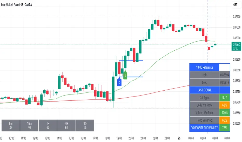
Institutional Sessions Overlay (Asia/London/NY)Institutional Sessions Overlay is a professional TradingView indicator that visually highlights the main trading sessions (Asia, London, and New York) directly on your chart.
Customizable: Easily adjust session start and end times (including minutes) for each market.
Timezone Alignment: Shift session boxes using the timezone offset parameter so sessions match your chart’s timezone exactly.
Clear Visuals: Colored boxes and optional labels display session opens and closes for fast institutional market structure reference.
Toggle Labels: Show or hide session open/close labels with a single click for a clean or detailed look.
Intuitive UI: User-friendly grouped settings for efficient configuration.
This tool is designed for day traders, institutional traders, and anyone who wants to instantly recognize global session timing and ranges for SMC, ICT, and other session-based strategies.
How to use:
Set your chart to your local timezone.
Use the "Session timezone offset" setting if session boxes do not match actual session opens on your chart.
Adjust the hours and minutes for each session as needed.
Enable or disable labels in the “Display” settings group.
Tip: Use the overlay to spot session highs and lows, volatility windows, and institutional liquidity sweeps.

KST Strategy [Skyrexio]Overview
KST Strategy leverages Know Sure Thing (KST) indicator in conjunction with the Williams Alligator and Moving average to obtain the high probability setups. KST is used for for having the high probability to enter in the direction of a current trend when momentum is rising, Alligator is used as a short term trend filter, while Moving average approximates the long term trend and allows trades only in its direction. Also strategy has the additional optional filter on Choppiness Index which does not allow trades if market is choppy, above the user-specified threshold. Strategy has the user specified take profit and stop-loss numbers, but multiplied by Average True Range (ATR) value on the moment when trade is open. The strategy opens only long trades.
Unique Features
ATR based stop-loss and take profit. Instead of fixed take profit and stop-loss percentage strategy utilizes user chosen numbers multiplied by ATR for its calculation.
Configurable Trading Periods. Users can tailor the strategy to specific market windows, adapting to different market conditions.
Optional Choppiness Index filter. Strategy allows to choose if it will use the filter trades with Choppiness Index and set up its threshold.
Methodology
The strategy opens long trade when the following price met the conditions:
Close price is above the Alligator's jaw line
Close price is above the filtering Moving average
KST line of Know Sure Thing indicator shall cross over its signal line (details in justification of methodology)
If the Choppiness Index filter is enabled its value shall be less than user defined threshold
When the long trade is executed algorithm defines the stop-loss level as the low minus user defined number, multiplied by ATR at the trade open candle. Also it defines take profit with close price plus user defined number, multiplied by ATR at the trade open candle. While trade is in progress, if high price on any candle above the calculated take profit level or low price is below the calculated stop loss level, trade is closed.
Strategy settings
In the inputs window user can setup the following strategy settings:
ATR Stop Loss (by default = 1.5, number of ATRs to calculate stop-loss level)
ATR Take Profit (by default = 3.5, number of ATRs to calculate take profit level)
Filter MA Type (by default = Least Squares MA, type of moving average which is used for filter MA)
Filter MA Length (by default = 200, length for filter MA calculation)
Enable Choppiness Index Filter (by default = true, setting to choose the optional filtering using Choppiness index)
Choppiness Index Threshold (by default = 50, Choppiness Index threshold, its value shall be below it to allow trades execution)
Choppiness Index Length (by default = 14, length used in Choppiness index calculation)
KST ROC Length #1 (by default = 10, value used in KST indicator calculation, more information in Justification of Methodology)
KST ROC Length #2 (by default = 15, value used in KST indicator calculation, more information in Justification of Methodology)
KST ROC Length #3 (by default = 20, value used in KST indicator calculation, more information in Justification of Methodology)
KST ROC Length #4 (by default = 30, value used in KST indicator calculation, more information in Justification of Methodology)
KST SMA Length #1 (by default = 10, value used in KST indicator calculation, more information in Justification of Methodology)
KST SMA Length #2 (by default = 10, value used in KST indicator calculation, more information in Justification of Methodology)
KST SMA Length #3 (by default = 10, value used in KST indicator calculation, more information in Justification of Methodology)
KST SMA Length #4 (by default = 15, value used in KST indicator calculation, more information in Justification of Methodology)
KST Signal Line Length (by default = 10, value used in KST indicator calculation, more information in Justification of Methodology)
User can choose the optimal parameters during backtesting on certain price chart.
Justification of Methodology
Before understanding why this particular combination of indicator has been chosen let's briefly explain what is KST, Williams Alligator, Moving Average, ATR and Choppiness Index.
The KST (Know Sure Thing) is a momentum oscillator developed by Martin Pring. It combines multiple Rate of Change (ROC) values, smoothed over different timeframes, to identify trend direction and momentum strength. First of all, what is ROC? ROC (Rate of Change) is a momentum indicator that measures the percentage change in price between the current price and the price a set number of periods ago.
ROC = 100 * (Current Price - Price N Periods Ago) / Price N Periods Ago
In our case N is the KST ROC Length inputs from settings, here we will calculate 4 different ROCs to obtain KST value:
KST = ROC1_smooth × 1 + ROC2_smooth × 2 + ROC3_smooth × 3 + ROC4_smooth × 4
ROC1 = ROC(close, KST ROC Length #1), smoothed by KST SMA Length #1,
ROC2 = ROC(close, KST ROC Length #2), smoothed by KST SMA Length #2,
ROC3 = ROC(close, KST ROC Length #3), smoothed by KST SMA Length #3,
ROC4 = ROC(close, KST ROC Length #4), smoothed by KST SMA Length #4
Also for this indicator the signal line is calculated:
Signal = SMA(KST, KST Signal Line Length)
When the KST line rises, it indicates increasing momentum and suggests that an upward trend may be developing. Conversely, when the KST line declines, it reflects weakening momentum and a potential downward trend. A crossover of the KST line above its signal line is considered a buy signal, while a crossover below the signal line is viewed as a sell signal. If the KST stays above zero, it indicates overall bullish momentum; if it remains below zero, it points to bearish momentum. The KST indicator smooths momentum across multiple timeframes, helping to reduce noise and provide clearer signals for medium- to long-term trends.
Next, let’s discuss the short-term trend filter, which combines the Williams Alligator and Williams Fractals. Williams Alligator
Developed by Bill Williams, the Alligator is a technical indicator that identifies trends and potential market reversals. It consists of three smoothed moving averages:
Jaw (Blue Line): The slowest of the three, based on a 13-period smoothed moving average shifted 8 bars ahead.
Teeth (Red Line): The medium-speed line, derived from an 8-period smoothed moving average shifted 5 bars forward.
Lips (Green Line): The fastest line, calculated using a 5-period smoothed moving average shifted 3 bars forward.
When the lines diverge and align in order, the "Alligator" is "awake," signaling a strong trend. When the lines overlap or intertwine, the "Alligator" is "asleep," indicating a range-bound or sideways market. This indicator helps traders determine when to enter or avoid trades.
The next indicator is Moving Average. It has a lot of different types which can be chosen to filter trades and the Least Squares MA is used by default settings. Let's briefly explain what is it.
The Least Squares Moving Average (LSMA) — also known as Linear Regression Moving Average — is a trend-following indicator that uses the least squares method to fit a straight line to the price data over a given period, then plots the value of that line at the most recent point. It draws the best-fitting straight line through the past N prices (using linear regression), and then takes the endpoint of that line as the value of the moving average for that bar. The LSMA aims to reduce lag and highlight the current trend more accurately than traditional moving averages like SMA or EMA.
Key Features:
It reacts faster to price changes than most moving averages.
It is smoother and less noisy than short-term EMAs.
It can be used to identify trend direction, momentum, and potential reversal points.
ATR (Average True Range) is a volatility indicator that measures how much an asset typically moves during a given period. It was introduced by J. Welles Wilder and is widely used to assess market volatility, not direction.
To calculate it first of all we need to get True Range (TR), this is the greatest value among:
High - Low
abs(High - Previous Close)
abs(Low - Previous Close)
ATR = MA(TR, n) , where n is number of periods for moving average, in our case equals 14.
ATR shows how much an asset moves on average per candle/bar. A higher ATR means more volatility; a lower ATR means a calmer market.
The Choppiness Index is a technical indicator that quantifies whether the market is trending or choppy (sideways). It doesn't indicate trend direction — only the strength or weakness of a trend. Higher Choppiness Index usually approximates the sideways market, while its low value tells us that there is a high probability of a trend.
Choppiness Index = 100 × log10(ΣATR(n) / (MaxHigh(n) - MinLow(n))) / log10(n)
where:
ΣATR(n) = sum of the Average True Range over n periods
MaxHigh(n) = highest high over n periods
MinLow(n) = lowest low over n periods
log10 = base-10 logarithm
Now let's understand how these indicators work in conjunction and why they were chosen for this strategy. KST indicator approximates current momentum, when it is rising and KST line crosses over the signal line there is high probability that short term trend is reversing to the upside and strategy allows to take part in this potential move. Alligator's jaw (blue) line is used as an approximation of a short term trend, taking trades only above it we want to avoid trading against trend to increase probability that long trade is going to be winning.
Almost the same for Moving Average, but it approximates the long term trend, this is just the additional filter. If we trade in the direction of the long term trend we increase probability that higher risk to reward trade will hit the take profit. Choppiness index is the optional filter, but if it turned on it is used for approximating if now market is in sideways or in trend. On the range bounded market the potential moves are restricted. We want to decrease probability opening trades in such condition avoiding trades if this index is above threshold value.
When trade is open script sets the stop loss and take profit targets. ATR approximates the current volatility, so we can make a decision when to exit a trade based on current market condition, it can increase the probability that strategy will avoid the excessive stop loss hits, but anyway user can setup how many ATRs to use as a stop loss and take profit target. As was said in the Methodology stop loss level is obtained by subtracting number of ATRs from trade opening candle low, while take profit by adding to this candle's close.
Backtest Results
Operating window: Date range of backtests is 2023.01.01 - 2025.05.01. It is chosen to let the strategy to close all opened positions.
Commission and Slippage: Includes a standard Binance commission of 0.1% and accounts for possible slippage over 5 ticks.
Initial capital: 10000 USDT
Percent of capital used in every trade: 60%
Maximum Single Position Loss: -5.53%
Maximum Single Profit: +8.35%
Net Profit: +5175.20 USDT (+51.75%)
Total Trades: 120 (56.67% win rate)
Profit Factor: 1.747
Maximum Accumulated Loss: 1039.89 USDT (-9.1%)
Average Profit per Trade: 43.13 USDT (+0.6%)
Average Trade Duration: 27 hours
These results are obtained with realistic parameters representing trading conditions observed at major exchanges such as Binance and with realistic trading portfolio usage parameters.
How to Use
Add the script to favorites for easy access.
Apply to the desired timeframe and chart (optimal performance observed on 1h BTC/USDT).
Configure settings using the dropdown choice list in the built-in menu.
Set up alerts to automate strategy positions through web hook with the text: {{strategy.order.alert_message}}
Disclaimer:
Educational and informational tool reflecting Skyrexio commitment to informed trading. Past performance does not guarantee future results. Test strategies in a simulated environment before live implementation.
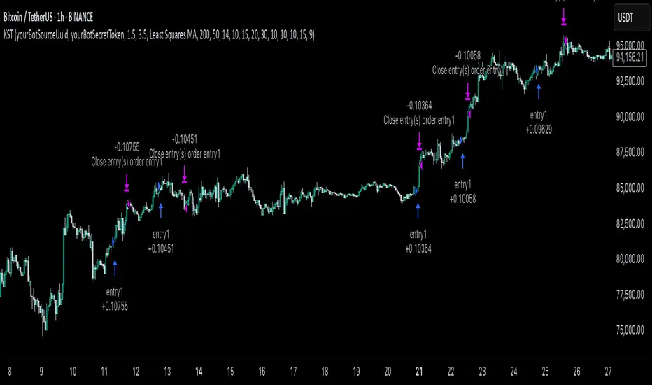
Aftershock Playbook: Stock Earnings Drift EngineStrategy type
Event-driven post-earnings momentum engine (long/short) built for single-stock charts or ADRs that publish quarterly results.
What it does
Detects the exact earnings bar (request.earnings, lookahead_off).
Scores the surprise and launches a position on that candle’s close.
Tracks PnL: if the first leg closes green, the engine automatically re-enters on the very next bar, milking residual drift.
Blocks mid-cycle trades after a loss until the next earnings release—keeping the risk contained to one cycle.
Think of it as a sniper that fires on the earnings pop, reloads once if the shot lands, then goes silent until the next report.
Core signal inputs
Component Default Purpose
EPS Surprise % +0 % / –5 % Minimum positive / negative shock to trigger longs/shorts.
Reverse signals? Off Quick flip for mean-reversion experiments.
Time Risk Mgt. Off Optional hard exit after 45 calendar days (auto-scaled to any TF).
Risk engine
ATR-based stop (ATR × 2 by default, editable).
Bar time stop (15-min → Daily: Have to select the bar value ).
No pyramiding beyond the built-in “double-tap”.
All positions sized as % of equity via Strategy Properties.
Visual aids
Yellow triangle marks the earnings bar.
Diagnostics table (top-right) shows last Actual, Estimate, and Surprise %.
Status-line tool-tips on every input.
Default inputs
Setting Value
Positive surprise ≥ 0 %
Negative surprise ≤ –5 %
ATR stop × 2
ATR length 50
Hold horizon 350 ( 1h timeframe chart bars)
Back-test properties
Initial capital 10 000
Order size 5 % of equity
Pyramiding 1 (internal re-entry only)
Commission 0.03 %
Slippage 5 ticks
Fills Bar magnifier ✔ · On bar close ✔ · Standard OHLC ✔
How to use
Add the script to any earnings-driven stock (AAPL, MSFT, TSLA…).
Turn on Time Risk Management if you want stricter risk management
Back-test different ATR multipliers to fit the stock’s volatility.
Sync commission & slippage with your broker before forward-testing.
Important notes
Works on every timeframe from 15 min to 1 D. Sweet spot around 30min/1h
All request.earnings() & request.security() calls use lookahead_off—zero repaint.
The “double-tap” re-entry occurs once per winning cycle to avoid drift-chasing loops.
Historical stats ≠ future performance. Size positions responsibly.
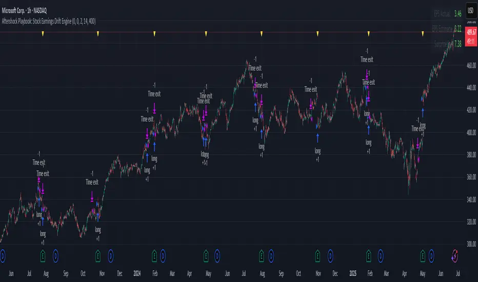
Out of the Noise Intraday Strategy with VWAP [YuL]This is my (naive) implementation of "Beat the Market An Effective Intraday Momentum Strategy for S&P500 ETF (SPY)" paper by Carlo Zarattini, Andrew Aziz, Andrea Barbon, so the credit goes to them.
It is supposed to run on SPY on 30-minute timeframe, there may be issues on other timeframes.
I've used settings that were used by the authors in the original paper to keep it close to the publication, but I understand that they are very aggressive and probably shouldn't be used like that.
Results are good, but not as good as they are stated in the paper (unsurprisingly?): returns are smaller and Sharpe is very low (which is actually weird given the returns and drawdown ratio), there are also margin calls if you enable margin check (and you should).
I have my own ideas of improvements which I will probably implement separately to keep this clean.
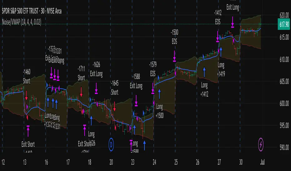
Double Bottom Strategy (Long Only, ATR Trailing Stop + Alerts)This script implements a long-only breakout strategy based on the recognition of a Double Bottom price pattern, enhanced with a 50 EMA trend filter and a dynamic ATR-based trailing stop. It is suitable for traders looking to capture reversals in trending markets using a structured pattern-based entry system.
🧠 Key Features:
Double Bottom Detection: Identifies double bottom structures using pivot lows with configurable tolerance.
ATR-Based Trailing Stop: Manages exits using a trailing stop calculated from Average True Range (ATR), dynamically adjusting to market volatility.
EMA Filter (Optional): Filters trades to only go long when price is above the 50 EMA (trend confirmation).
Alerts: Real-time alerts on entry and exit, formatted in JSON for webhook compatibility.
Backtest Range Controls: Customize historical testing period with start and end dates.
✅ Recommended Markets:
Gold (XAUUSD)
S&P 500 (SPX, ES)
Nasdaq (NDX, NQ)
Stocks (Equities)
⚠️ Not recommended for Forex due to differing behavior and noise levels in currency markets.
🛠️ User Guidance:
Tune the pivot period, tolerance, and ATR settings for best performance on your chosen asset.
Backtest thoroughly over your selected date range to assess historical effectiveness.
Use small position sizes initially to test viability in live or simulated environments.
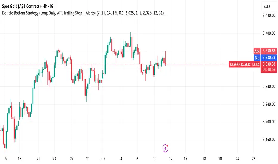
PRO Trading Averaging Beta(v1)Adaptive Position Scaling
Automatically increases position size during pullbacks using exponential volume scaling (1x, 2x, 4x, etc.). This reduces average entry cost and accelerates breakeven when price reverses.
Multi-Timeframe Confirmation
All indicators operate on a higher timeframe (120 minutes), providing:
Noise-filtered signals
Stronger trend alignment
Reduced false entries
Triple-Layer Entry Logic
Requires simultaneous confluence of:
Custom Bollinger Band penetration
RSI oversold filter (above critical threshold)
Golden cross confirmation (fast MA > slow MA)
Volatility assessment via ATR
Intelligent Exit System
Position closure triggers when either:
Fixed profit target (% of account) is reached
Technical boundary (upper Bollinger Band) is touched
⚙️ Core Mechanics:
graph LR
A --> B
B --> C{Initial Entry: 1% capital}
C --> D
D -->|Yes| E
D -->|No| F
E --> G{Max Averaging Levels?}
G -->|No| D
G -->|Yes| H
F --> I
📊 Implementation Guide:
Capital Configuration
Set initial_capital to your actual account size
Calculate base contract size:
(Account Size × 0.01) / (Instrument Price × Point Value)
Example: $10,000 account → 0.01 BTC futures contracts
Pyramiding Structure
Volume progression per averaging level:
Level 1: 1× (Base volume)
Level 2: 2×
Level 3: 4×
Level 4: 8×
Level 5: 16×
Level 6: 32×
(Max 6 levels configurable in strategy settings)
Custom Entry Variations
Alternative approach for swing captures:
// Enter only at 3rd averaging with 5% capital
if averaging_condition and strategy.opentrades == 2
strategy.entry("SwingEntry", strategy.long, qty=base_order_size*5)
Risk Management Protocol
No traditional stop-loss (replaced by averaging)
Break-even trigger: Manually move to breakeven at +0.5% profit
Max exposure: Capped at 6 averaging levels
Commissions: Pre-configured at 0.1% per trade
⚠️ Critical Risk Disclosures:
"Past Performance ≠ Future Results"
Historical optimization requires continuous forward testing ("Walk Forward" in TV).
Pyramiding Hazards
Exponential volume growth demands:
Minimum 20% free margin buffer
High liquidity instruments (spread < 0.5% of ATR)
Strict per-level risk calculation
Market Regime Dependence
Peak efficiency during:
Strong trends with 2-4% retracements
Assets with ATR > 1.5% of daily range
Avoid ranging/low-volatility conditions
💡 Pro Usage Recommendations:
Position Sizing Formula
For futures: Contracts = (Capital × Risk %) / (Entry Price × Point Value × Stop Distance)
Profit Protection
Close 50% position at 50% profit target, trail remainder
Event Safety
Disable averaging during:
High-impact news events
Exchange outages
Abnormal volume spikes
pie
title Risk Allocation per Level
“First Entry” : 12
“Level 2” : 18
“Level 3” : 25
“Level 4” : 45
ESSENTIAL: This strategy demands strict discipline. Terminate averaging when price action deviates from expected patterns. Always maintain reserve capital exceeding maximum drawdown requirements. Regularly validate strategy performance against current market dynamics.
🔥 Уникальные особенности и ценность:
Адаптивное усреднение
Стратегия автоматически увеличивает позицию при движении против вас, используя экспоненциальное наращивание объема (1x, 2x, 4x и т.д.). Это снижает среднюю цену входа и ускоряет выход в прибыль при развороте.
Мультитаймфреймная фильтрация
Все индикаторы работают на старшем таймфрейме (120 минут), что:
Фильтрует рыночный шум
Обеспечивает более надежные сигналы
Синхронизируется с глобальным трендом
Комбинированный триггер входа
Для активации требуется одновременное выполнение 4 условий:
Пробитие кастомной полосы Боллинджера
Подтверждение тренда (быстрая MA > медленной MA)
Контроль перепроданности (RSI выше критического уровня)
Фильтр волатильности (ATR)
Двойной механизм выхода
Закрытие позиций происходит при:
Достижении целевого уровня прибыли (% от депозита)
Техническом сигнале (касание верхней полосы Боллинджера)
⚙️ Как работает стратегия:
graph TD
A --> B
B --> C{Первый вход: 1% депозита}
C --> D
D -->|Да| E
D -->|Нет| F
E --> G{Достигнут лимит усреднений?}
G -->|Нет| D
G -->|Да| H
F --> I
📊 Как пользоваться:
Стартовые настройки
Base Order Size: Стартовый объем = 1% депозита
(Пример: при $10 000 депозита = 0.01 контракта)
initial_capital: Укажите ваш реальный депозит
Правила пирамидинга
Объем наращивается по схеме:
Уровень 1: 1x (базовый объем)
Уровень 2: 2x
Уровень 3: 4x
Уровень 4: 8x
Уровень 5: 16x
Уровень 6: 32x
РЕКОМЕНДУЕТСЯ Максимум 6 уровней усреднения (настраивается в pyramiding)
Кастомизация входов
Пример модификации для агрессивной тактики:
// Вход только на 3-м усреднении с 5% депозита
if averaging_condition and strategy.opentrades == 2
strategy.entry("BuyAggressive", strategy.long, qty=base_order_size*5)
Можно поставить параметр пираммидинг 1 и получать больше сигналов на младших тайм фреймах
Управление рисками
Стоп-лосс: Не используется (заменен усреднением)
Перевод в безубыток: Активируйте вручную при +0.5%
Максимальная просадка: Рекомендуется Ограничивать 6 уровнями усреднения
Комиссии: Учтены (0.1% от объема сделки)
Критические предупреждения:
"Вчера ≠ Сегодня"
Стратегия оптимизирована под историческую волатильность. Регулярно тестируйте на новых данных (режим "Перед тест" в TV).
Опасность усреднения
Экспоненциальный рост объема требует:
Глубокого расчета риска на уровень
Минимум 20% свободного маржи
Ликвидный инструмент (спред < 0.5% от ATR)
Рыночные условия
Максимальная эффективность в:
Трендовых рынках с коррекциями 2-4%
Инструментах с ATR > дневного диапазона 1.5%
💡 Рекомендации по использованию:
Для фьючерсов: Рассчитайте контракты через (капитал * 0.01) / (цена * пункт_стоимости)
При 50% достижении цели прибыли - закройте 50% позиции
Отключайте усреднение при выходе макро-новостей
pie
title Распределение риска
"Первый вход" : 10
"Уровень 2" : 20
"Уровень 3" : 30
"Уровень 4" : 40
ВАЖНО: Эта стратегия требует дисциплины! Прекращайте усреднение при отклонении рынка от исторических паттернов. Всегда имейте резервный капитал для экстренных случаев.

Price Statistical Strategy-Z Score V 1.01
Price Statistical Strategy – Z Score V 1.01
Overview
A technical breakdown of the logic and components of the “Price Statistical Strategy – Z Score V 1.01”.
This script implements a smoothed Z-Score crossover mechanism applied to the closing price to detect potential statistical deviations from local price mean. The strategy operates solely on price data (close) and includes signal spacing control and momentum-based candle filters. No volume-based or trend-detection components are included.
Core Methodology
The strategy is built on the statistical concept of Z-Score, which quantifies how far a value (closing price) is from its recent average, normalized by standard deviation. Two moving averages of the raw Z-Score are calculated: a short-term and a long-term smoothed version. The crossover between them generates long entries and exits.
Signal Conditions
Entry Condition:
A long position is opened when the short-term smoothed Z-Score crosses above the long-term smoothed Z-Score, and additional entry conditions are met.
Exit Condition:
The position is closed when the short-term Z-Score crosses below the long-term Z-Score, provided the exit conditions allow.
Signal Gapping:
A minimum number of bars (Bars gap between identical signals) must pass between repeated entry or exit signals to reduce noise.
Momentum Filter:
Entries are prevented during sequences of three or more consecutively bullish candles, and exits are prevented during three or more consecutively bearish candles.
Z-Score Function
The Z-Score is calculated as:
Z = (Close - SMA(Close, N)) / STDEV(Close, N)
Where N is the base period selected by the user.
Input Parameters
Enable Smoothed Z-Score Strategy
Enables or disables the Z-Score strategy logic. When disabled, no trades are executed.
Z-Score Base Period
Defines the number of bars used to calculate the simple moving average and standard deviation for the Z-Score. This value affects how responsive the raw Z-Score is to price changes.
Short-Term Smoothing
Sets the smoothing window for the short-term Z-Score. Higher values produce smoother short-term signals, reducing sensitivity to short-term volatility.
Long-Term Smoothing
Sets the smoothing window for the long-term Z-Score, which acts as the reference line in the crossover logic.
Bars gap between identical signals
Minimum number of bars that must pass before another signal of the same type (entry or exit) is allowed. This helps reduce redundant or overly frequent signals.
Trade Visualization Table
A table positioned at the bottom-right displays live PnL for open trades:
Entry Price
Unrealized PnL %
Text colors adapt based on whether unrealized profit is positive, negative, or neutral.
Technical Notes
This strategy uses only close prices — no trend indicators or volume components are applied.
All calculations are based on simple moving averages and standard deviation over user-defined windows.
Designed as a minimal, isolated Z-Score engine without confirmation filters or multi-factor triggers.