Pressure Pivots - MPI (Strategy)⇋ PRESSURE PIVOTS — MARKET PRESSURE INDEX STRATEGY
A comprehensive reversal trading system that combines order flow pressure analysis, multi-factor confluence detection, and adaptive machine learning to identify high-probability turning points in liquid markets.
━━━━━━━━━━━━━━━━━━━━━━━━━━━━━━━━━━━━━
CORE INNOVATION: MARKET PRESSURE INDEX (MPI)
Traditional indicators measure price movement. The Market Pressure Index measures the force behind the movement.
How MPI Works:
Every bar tells two stories through volume distribution:
• Buy Pressure: Volume × (Close - Low) / (High - Low)
• Sell Pressure: Volume × (High - Close) / (High - Low)
• Net Pressure: Buy Pressure - Sell Pressure
This raw pressure is then normalized against baseline activity to create the bounded MPI (-1.0 to +1.0):
• Smooth Pressure: EMA(Net Pressure, period)
• Baseline Activity: SMA(|Net Pressure|, period × 2)
• MPI: (Smooth Pressure / Baseline) × Sensitivity
What MPI Reveals:
MPI > +0.7: Extreme buy pressure → Exhaustion potential
MPI = +0.2 to +0.7: Healthy bullish momentum
MPI = -0.2 to +0.2: Neutral/balanced pressure
MPI = -0.7 to -0.2: Healthy bearish momentum
MPI < -0.7: Extreme sell pressure → Exhaustion potential
Why It Works:
Two bars can both move 10 points, but if one closes at the high on high volume (aggressive buying) and the other closes mid-range on average volume (weak buying), only MPI distinguishes between sustainable momentum and exhaustion. This volume-weighted pressure analysis reveals conviction behind price moves—the key to timing reversals.
━━━━━━━━━━━━━━━━━━━━━━━━━━━━━━━━━━━━━
SEVEN-FACTOR CONFLUENCE SYSTEM
MPI extremes alone aren't enough. The system requires multiple independent confirmations through weighted scoring:
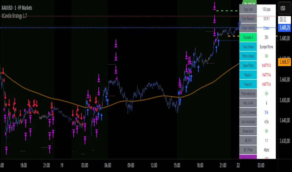
1. DIVERGENCE (Weight: 3.0) — Premium Signal Type: DIV
Price makes new high but MPI makes lower high (or inverse for bullish)
• Detection: Tracks pivots with 5-bar lookback, compares price vs MPI at pivot points
• Signal: Purple triangles, highest weight (pressure weakening while price extends)
2. LIQUIDITY SWEEP (Weight: 2.5) — Premium Signal Type: LIQ
Price breaks swing high/low within 0.3 ATR then reverses
• Detection: Break within tolerance + close back through level
• Signal: Orange triangles, second-highest weight (stop hunt reversal)
3. ORDER FLOW IMBALANCE (Weight: 2.0) — Premium Signal Type: OF
Aggressive buying/selling 50% above normal
• Detection: EMA(aggressive volume) vs SMA(imbalance) threshold
• Signal: Aqua triangles, institutional positioning
4. VELOCITY EXHAUSTION (Weight: 1.5)
Parabolic move (2+ ATRs in 3 bars) + extreme MPI
• Detection: |3-bar price change / ATR| > threshold + MPI > ±0.5
• Indicates: Momentum deceleration, blow-off top/bottom
5. WICK REJECTION (Weight: 1.5)
Single bar: wick > 60% of range, or sequence: 2 bars with 40% + 30% wicks
• Detection: Shooting stars (bearish) or hammers (bullish)
• Indicates: Intrabar rejection, battle won by opposing side
6. VOLUME SPIKE (Weight: 1.0)
Volume > 20-bar average × multiplier (default: 2.0x)
• Detection: Participation surge confirmation
• Lowest weight: Can be manipulated, better as confirmation
7. POSITION FACTOR (Weight: 1.0)
At 10-bar highest (bearish) or lowest (bullish)
• Detection: Structural positioning for reversal
• Base requirement: Must be at extreme to score
Scoring Logic:
Premium Signals (DIV/LIQ/OF): Must score ≥6.0 (default premiumThreshold)
Standard Signals (STD): Must score ≥4.0 (default standardThreshold)
Example Scoring:
Divergence (3.0) + Liquidity Sweep (2.5) + Volume (1.0) = 6.5 → FIRES (DIV signal)
Recent High (1.0) + Wick (1.5) + Volume (1.0) + Velocity (1.5) = 5.0 → FIRES (STD signal)
━━━━━━━━━━━━━━━━━━━━━━━━━━━━━━━━━━━━━
ADAPTIVE LEARNING ENGINE
Unlike static strategies, this system learns from every trade and optimizes itself.
Performance Tracking:
Every trade records:
• Entry Score: Confluence level at entry
• Signal Type: DIV / LIQ / OF / STD
• Win/Loss: Boolean outcome
• R-Multiple: (Exit - Entry) / (Entry - Stop)
• MAE: Maximum Adverse Excursion (worst drawdown)
• MFE: Maximum Favorable Excursion (best profit reached)
Three Adaptive Parameters:
1. Signal Threshold Adaptation
If Win Rate < Target (45%): RAISE threshold → fewer signals, better quality
If Win Rate > Target + 10% AND good R: LOWER threshold → more signals, profitable
2. Stop Distance Adaptation
If Avg MAE > 0.85 AND WR < 50%: WIDEN stops → reduce premature exits
If Avg MAE < 0.4 AND WR > 55%: TIGHTEN stops → reduce risk
3. Target Distance Adaptation
If Avg MFE > Target × 1.5: EXTEND targets → capture more of runners
If Avg MFE < Target × 0.7: SHORTEN targets → take profits faster
Signal Type Filtering:
The system tracks performance by type (DIV/LIQ/OF/STD):
• If Type WR < 40% AND Avg R < 0.8: Type DISABLED
• If Type WR ≥ 40% OR Avg R ≥ 0.8: Type RE-ENABLED
Example: If OF signals consistently lose while DIV signals win, system automatically stops taking OF signals and focuses on DIV.
Warmup Period:
First 30 trades (default) gather baseline data with relaxed thresholds. After warmup, full adaptation activates.
━━━━━━━━━━━━━━━━━━━━━━━━━━━━━━━━━━━━━
COMPLETE POSITION MANAGEMENT
Dynamic Position Sizing:
Base Contracts = (Equity × Risk%) / (Stop Distance × Point Value)
Then multiplied by:
• Score Bonus: Up to +50% for highest-scoring signals
• Signal Type Bonus: DIV signals +50%, LIQ signals +30%
• Streak Multiplier: After 3 losses: 50% reduction, After 3 wins: 25% increase
Example: High-scoring DIV signal on winning streak = 3-4× larger position than weak STD signal on losing streak
Entry Modes:
Single Entry: Full size at once, exit at TP2 (or partial at TP1)
Tiered Entry: 40% at TP1 (2R), 60% at TP2 (4R adaptive)
Stop Management (3 Modes):
Structural: Beyond recent 20-bar swing high/low + buffer
ATR: Fixed ATR multiplier (default: 2.0 ATR, then adapts)
Hybrid: Attempt structural, fallback to ATR if invalid
Plus:
• Breakeven: Move stop to entry ± 1 tick when 1R reached
• Trailing: Activate when 1.5R reached, trail 0.8R behind price
• Max Loss Override: Cap dollar risk regardless of calculation
Target Management:
Fixed Mode: TP1 = 2R, TP2 = 4R
Adaptive Mode: TP1 = 2R fixed, TP2 adapts based on MFE analysis
Partial Exits: Default 50% at TP1, remainder at TP2 or trailing stop
━━━━━━━━━━━━━━━━━━━━━━━━━━━━━━━━━━━━━
COMPREHENSIVE RISK CONTROLS
Daily Limits:
• Max Daily Loss: $2,000 default → HALT trading
• Max Daily Trades: 15 default → prevent overtrading
• Max Concurrent: 2 positions → limit correlation risk
Session Controls:
• Trading Hours: Specify start/end times + timezone
• Weekend Block: Optional (avoid crypto weekend volatility)
Prop Firm Protection (Live Trading Only):
• Daily Loss Limit: Stricter of general or prop limit ($1,000 default)
• Trailing Drawdown: Tracks high water mark, HALTS if breach ($2,500 default)
• Reset on Reload: Optional high water mark reset
Liquidity Filter (Optional):
• Time-Based: Avoid first/last X minutes of session
• Volume-Based: Require minimum volume ratio (0.5× average default)
Market Regime Filter (Optional):
• ADX-Based: Only trade when ADX > threshold (trending)
• Block: Consolidation (ADX < 20) or Transitional regimes
━━━━━━━━━━━━━━━━━━━━━━━━━━━━━━━━━━━━━
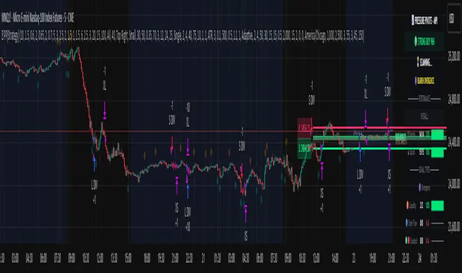
REAL-TIME DASHBOARD
MPI Gauge Section:
Shows current pressure: 🟢 STRONG BUY (+0.5 to +1.0), 🟩 BUY PRESSURE (+0.2 to +0.5), ⚪ NEUTRAL (-0.2 to +0.2), 🟥 SELL PRESSURE (-0.5 to -0.2), 🔴 STRONG SELL (-1.0 to -0.5)
Signal Status Section:
• Active Signals: "🔴 DIV SELL" (purple background), "🟢 LIQ BUY" (orange), "🔵 OF SELL" (aqua), "🟢 STD BUY" (green)
• Warnings: "⚠️ BEAR WARNING" / "⚠️ BULL WARNING" (yellow) — setup forming, not full signal
• Scanning: "⏳ SCANNING..." (gray) — no signal active
• Confidence Bar: Visual score display "██████░░░░" showing confluence strength
Divergence Indicator:
"🟣 BEARISH DIVERGENCE" or "🟡 BULLISH DIVERGENCE" when detected
Performance Statistics:
• Overall Win Rate: Wins/Total with visual bar (lime ≥70%, yellow 50-70%, red <50%)
• Directional: Bearish vs Bullish win rates separately
• By Signal Type: DIV / LIQ / OF / STD individual performance tracking
━━━━━━━━━━━━━━━━━━━━━━━━━━━━━━━━━━━━━
KEY PARAMETERS EXPLAINED
🎯 Pressure Engine:
• MPI Period (5-50, default: 14): Smoothing period — lower for scalping, higher for position trading
• MPI Sensitivity (0.5-5.0, default: 1.5): Amplification — lower compresses range, higher more extremes
🔍 Detection:
• Wick Threshold (0.3-0.9, default: 0.6): Minimum wick-to-range ratio for rejection
• Volume Spike (1.2-3.0x, default: 2.0): Multiplier above average for spike
• Aggressive Ratio (0.5-0.9, default: 0.65): Close position in range for aggressive orders
• Velocity Threshold (1.0-5.0 ATR, default: 2.0): ATR-normalized move for exhaustion
• MPI Extreme (0.5-0.95, default: 0.7): Level considered overbought/oversold
⚖️ Weights:
• Divergence: 3.0 (highest — pressure weakening)
• Liquidity: 2.5 (second — stop hunts)
• Order Flow: 2.0 (institutional positioning)
• Velocity: 1.5 (momentum exhaustion)
• Wick: 1.5 (rejection patterns)
• Volume: 1.0 (lowest — can be manipulated)
🎚️ Thresholds:
• Premium (4.0-15.0, default: 6.0): Score for DIV/LIQ/OF signals
• Standard (2.0-8.0, default: 4.0): Score for STD signals
• Warning Confluence (1-4, default: 2): Factors for yellow diamond warnings
🧬 Adaptive:
• Enable (true/false, default: true): Master learning switch
• Warmup Trades (5-100, default: 30): Data collection before adaptation
• Lookback (20-200, default: 50): Recent trades for performance calculation
• Adapt Speed (0.05-0.50, default: 0.15): Parameter adjustment rate
• Target Win Rate (30-70%, default: 45%): Optimization goal
• Target R-Multiple (0.5-5.0, default: 1.5): Risk/reward goal
💼 Position:
• Base Risk (0.1-10.0%, default: 1.5%): Equity risked per trade
• Max Contracts (1-100, default: 10): Hard position limit
• DIV Bonus (1.0-3.0x, default: 1.5): Size multiplier for divergence signals
• LIQ Bonus (1.0-3.0x, default: 1.3): Size multiplier for liquidity signals
🛡️ Stops:
• Mode (Structural/ATR/Hybrid, default: ATR): Stop placement method
• ATR Multiplier (0.5-5.0, default: 2.0): Stop distance in ATRs (adapts)
• Breakeven at (0.3-3.0R, default: 1.0R): When to move stop to entry
• Trail Trigger (0.5-5.0R, default: 1.5R): When to activate trailing
• Trail Offset (0.3-3.0R, default: 0.8R): Distance behind price
🎯 Targets:
• Mode (Fixed/Adaptive, default: Fixed): Target placement method
• TP1 (0.5-10.0R, default: 2.0R): First target for partial exit
• TP2 (1.0-15.0R, default: 4.0R): Final target (adapts in adaptive mode)
• Partial % (0-100%, default: 50%): Position percentage to exit at TP1
━━━━━━━━━━━━━━━━━━━━━━━━━━━━━━━━━━━━━
PROFESSIONAL USAGE PROTOCOL
Phase 1: Paper Trading (Weeks 1-4)
• Setup: Default settings, all adaptive features ON, 0.5% base risk
• Goal: 30+ trades for warmup, observe MPI behavior and signal frequency
• Adjust: MPI sensitivity if stuck near neutral or always at extremes
• Threshold: Raise/lower if too many/few signals
Phase 2: Micro Live (Weeks 5-8)
• Requirements: WR >43%, at least one type >55%, Avg R >0.8
• Setup: 10-25% intended size, 0.5-1.0% risk, 1 position max
• Focus: Execution quality, match dashboard performance
• Journal: Screenshot every signal, track outcomes
Phase 3: Full Scale (Month 3+)
• Requirements: WR >45% over 50+ trades, Avg R >1.2, drawdown <15%
• Progression: Months 3-4 (1.0-1.5% risk), 5-6 (1.5-2.0%), 7+ (1.5-2.5%)
• Maintenance: Weekly dashboard review, monthly deep analysis
• Warnings: Reduce size if WR drops >10%, consecutive losses >7, or drawdown >20%
━━━━━━━━━━━━━━━━━━━━━━━━━━━━━━━━━━━━━
DEVELOPMENT INSIGHTS
The Pressure Insight: Emerged from analyzing intrabar volume distribution. Within every candlestick, volume accumulates at different price levels. MPI deconstructs this to reveal conviction behind moves.
The Confluence Challenge: Early versions using MPI extremes alone achieved only 42% win rate. The seven-factor confluence system emerged from testing which combinations produced reliable reversals. Divergence + liquidity sweep became the strongest setup (68% win rate in isolation).
The Adaptive Breakthrough: Per-signal-type performance tracking revealed DIV signals winning at 71% while OF signals languished at 38%. Adaptive filtering disabled weak types automatically, recovering win rate from 39% to 54% during the 2022 volatility spike.
The Position Sizing Revelation: Dynamic sizing based on signal quality and recent performance increased Sharpe ratio from 1.2 to 1.9 while decreasing max drawdown from 18% to 12% over 500 trades. Bigger positions on better signals = geometric edge amplification.
The Risk Control Lesson: Testing with $50K accounts revealed catastrophic failure modes: daily loss cascades, overtrading commission bleed, weekend gap blowouts. Multi-layer controls (daily limits, concurrent caps, prop firm protection) became essential.
━━━━━━━━━━━━━━━━━━━━━━━━━━━━━━━━━━━━━
LIMITATIONS & ASSUMPTIONS
What This Is NOT:
• NOT a Holy Grail: Typical performance 52-58% WR, 1.3-1.8 avg R, probabilistic edge
• NOT Predictive: Identifies high-probability conditions, doesn't forecast prices
• NOT Market-Agnostic: Best on liquid auction-driven markets (futures, forex, major crypto)
• NOT Hands-Off: Requires oversight for news events, gaps, system anomalies
• NOT Immune to Regime Changes: Adaptive engine helps but cannot predict black swans
Critical Assumptions:
1. Volume reflects intent (valid for regulated markets, violated by wash trading)
2. Pressure extremes mean-revert (true in ranging/exhaustion, fails in paradigm shifts)
3. Stop hunts exist (valid in liquid markets, less in thin/random walk periods)
4. Past patterns persist (valid in stable regimes, fails when structure fundamentally changes)
Works Best On: Major futures (ES, NQ, CL), liquid forex pairs (EUR/USD, GBP/USD), large-cap stocks, BTC
Performs Poorly On: Low-volume stocks, illiquid crypto pairs, news-driven headline events
━━━━━━━━━━━━━━━━━━━━━━━━━━━━━━━━━━━━━
RISK DISCLOSURE
Trading futures, forex, and leveraged instruments involves substantial risk of loss and is not suitable for all investors. Past performance is not indicative of future results. This strategy is provided for educational purposes only and should not be construed as financial advice.
The adaptive engine learns from historical data—there is no guarantee that past relationships will persist. Market conditions change, volatility regimes shift, and black swan events occur. No strategy can eliminate the risk of loss.
Users must validate performance on their specific instruments and timeframes before risking capital. The developer makes no warranties regarding profitability or suitability. Users assume all responsibility for trading decisions and outcomes.
"The market doesn't care about your indicators. It only cares about pressure—who's willing to pay more, who's desperate to sell. Find the exhaustion. Trade the reversal. Let the system learn the rest."
Taking you to school. — Dskyz, Trade with insight. Trade with anticipation.
Pine Script® stratejisi