Blackflag FTS (1H Trailing) + MSB-OB FibThis indicator combines a 1-hour trailing stop system with multi-timeframe Fibonacci retracement levels and ZigZag structure detection to assist traders in identifying trend direction and potential reversal zones.
Features:
✅ 1-Hour Trailing Stop: Uses an ATR-based trailing stop mechanism to track trend direction and dynamic support/resistance.
✅ Multi-Timeframe Approach: The trailing stop is calculated on the 1-hour timeframe, while the ZigZag and Fibonacci retracement levels are based on the 15-minute chart.
✅ ZigZag Structure Detection: Helps filter market swings and trend reversals dynamically.
✅ Fibonacci Levels (0.5 & 0.786): Key retracement levels to watch for price reactions.
✅ Alerts for Key Levels: Get notified when the price crosses important levels (1H trailing stop, Fib 0.5, Fib 0.786).
How It Works:
The trailing stop adapts dynamically based on ATR values and determines trend direction.
ZigZag detection filters out minor price movements to highlight major swing points.
Fibonacci levels are calculated based on ZigZag swings, helping traders spot potential reversal zones.
This tool is useful for trend-following traders, breakout traders, and Fibonacci-based strategies.
Let me know if you'd like any modifications! 🚀
Komut dosyalarını "通达信+选股公式+换手率+0.5+源码" için ara

PullBack_Level_HunterThis script creates an "Auto Fibonacci" indicator that automatically plots selected Fibonacci retracement levels on a chart, based on a defined lookback period. Users can choose from various Fibonacci levels (0.236, 0.382, 0.5, 0.618, or 0.786) via a dropdown input, allowing for quick adjustments to analysis.
**Key Features:**
1. **Fibonacci Level Selection:** Users can select from multiple Fibonacci levels (0.236, 0.382, 0.5, 0.618, and 0.786) for analysis.
2. **Lookback Period:** The script allows users to define a lookback period to determine the highest high and the lowest low for plotting Fibonacci levels.
3. **Fibonacci Level Calculation:** The Fibonacci levels are calculated using two functions:
- `fib_level`: Calculates the Fibonacci level based on the highest high and lowest low of the lookback period.
- `fib_level_from_current`: Calculates the Fibonacci level from the current candle’s high.
4. **Plotting:** The script plots the selected Fibonacci level on the chart, using a red line for the general Fibonacci level and a blue line for the level calculated from the current high.
5. **Dynamic Visualization:** The Fibonacci levels are drawn as step lines to clearly visualize price levels based on historical data and current price action.
This tool is ideal for traders who wish to quickly assess key Fibonacci levels for potential support or resistance within a customizable lookback period.

Fibonacci Extension Strt StrategyCore Logic and Steps:
Weekly Trend Identification:
Find the last significant Higher High (HH) and Lower Low (LL) or vice-versa on the Weekly timeframe.
Determine if it's an uptrend (HH followed by LL) or a downtrend (LL followed by HH).
Plot a Fibonacci Extension (or Retracement in reverse order) from the swing point determined to the other significant swing point.
Weekly Retracement Levels:
Display horizontal lines at the 0.236, 0.382, and 0.5 Fibonacci levels from the weekly extension.
Monitor price action on these levels.
Daily Confirmation:
When price hits the Fib levels, examine the Daily chart.
Look for a rejection wick (indicating the pull back is ending) on the identified weekly retracement levels.
Confirm that the price is indeed starting to continue in the direction of the original weekly trend.
Four-Hour Entry:
On the 4H timeframe, plot a new Fib Extension in the opposite direction of the weekly.
If it's an uptrend, the Fib is plotted from last swing low to its swing high. If the weekly trend was bearish the Fib will be plotted from last swing high to the swing low.
Generate an entry when price breaks the high of that candle.
Trade Management:
Entry is on the breakout of the current candle.
Stop Loss: Place the stop loss below the wick of the breakout candle.
Take Profit 1: Close 50% of the position at the 0.5 Fibonacci level. Move the stop loss to breakeven on this position.
Take Profit 2: Close another 25% of the position at the 0.236 Fib level.
Trailing Take Profit: Keep the last 25% open, using a trailing stop loss. (You'll need to define the logic for the trailing stop, e.g., trailing stop using the last high/low)
How to Use in TradingView:
Open a TradingView Chart.
Click on "Pine Editor" at the bottom.
Copy and paste the corrected Pine Script code.
Click "Add to Chart".
The indicator should now be displayed on your chart.
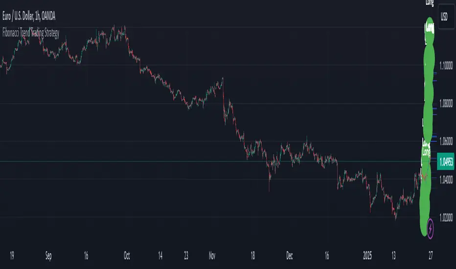
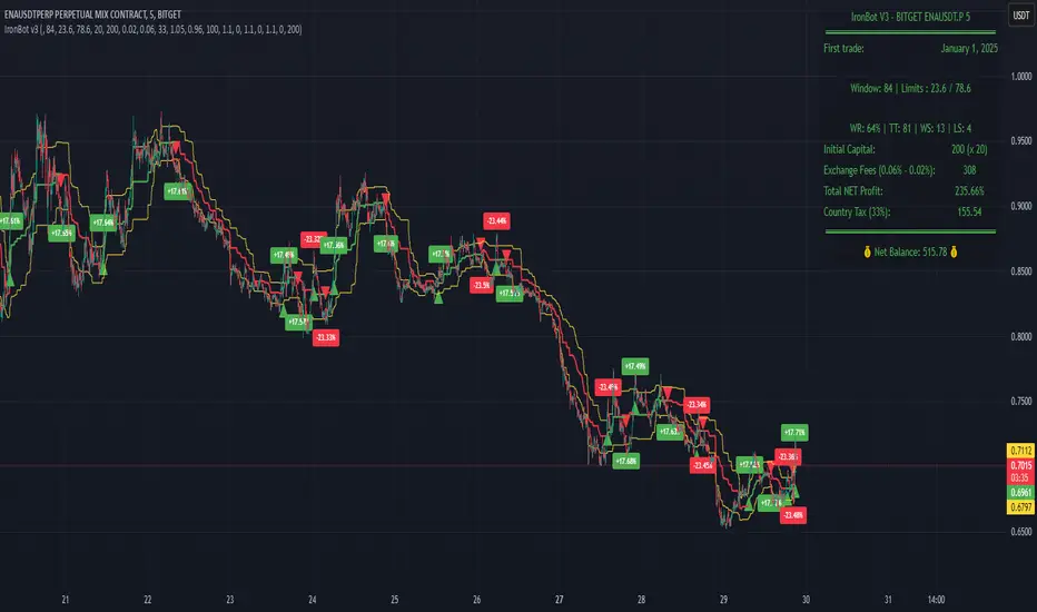
IronBot v3Introduction
IronBot V3 is a TradingView indicator that analyzes market trends, identifies potential trading opportunities, and helps manage trades by visualizing entry points, stop-loss levels, and take-profit targets.
How It Works
The indicator evaluates price action within a specified analysis window to determine market trends. It uses Fibonacci retracement levels to identify key price levels for trend detection and trading signals. Based on user-defined inputs, it calculates and displays trade levels, including entry points, stop-loss, and multiple take-profit levels.
Trend Definition:
The highest high and lowest low are calculated over a specified number of candles.
The price range is determined as the difference between the highest high and lowest low.
Three Fibonacci levels are calculated within this range:
- Fib Level 0.236
- Trend Line (0.5 level)
- Fib Level 0.786
Determining Long and Short Conditions:
Long Conditions (Buy):
The closing price must be above both the trend line (0.5 level) and the Fib Level 0.236.
Additionally, the market must not currently be in a bearish trend.
Short Conditions (Sell):
The closing price must be below both the trend line and the Fib Level 0.786.
The market must not currently be in a bullish trend.
Trend State Updates:
When a condition is met, the indicator sets the trend to bullish or bearish and turns off bearish or bullish trend conditions.
If neither buy nor sell conditions are met, the trend remains unchanged, and no new trade signals are generated.
Inputs and Their Role in the Algorithm
General Settings
Analysis Window: Specifies the number of historical candles to analyze. This influences the calculation of key levels such as highs and lows, which are critical for determining Fibonacci retracement levels.
First Trade: Defines the start date for generating trading signals.
Trade Configuration
Display TP/SL: Enables or disables the visualization of take-profit and stop-loss levels on the chart.
Leverage: Defines the leverage applied to trades for risk and position size calculations.
Initial Capital: Specifies the starting capital, which is used for calculating position sizes and profits.
Exchange Fees (%): Sets the percentage of fees applied by the exchange, which is factored into profit calculations.
Country Tax (%): Allows users to define applicable taxes, which are subtracted from net profits.
Stop-Loss Configuration
Break Even: Toggles the break-even functionality. When enabled, the stop-loss level adjusts dynamically as take-profit levels are reached.
Stop Loss (%): Defines the percentage distance from the entry price to the stop-loss level.
Take-Profit Settings
The indicator supports up to four take-profit levels:
- TP1 through TP4 Ratios: Specify the price levels for each take-profit target as a percentage of the entry price.
- Profit Percentages: Allocate a percentage of the position size to each take-profit level.
Visualization Elements
Trend Indicators: Displays Fibonacci-based trend lines and markers for bullish or bearish conditions.
Trade Levels: Entry, stop-loss, and take-profit levels are visualized on the chart by dotted lines for clarity. Additionally, a semi-transparent background is applied when a portion of the trade is closed to enhance visualization. Positive profits from a closed trade are green; otherwise, they are red.
Trade Profit Indicator: On each trade, every time a part of the trade is closed (e.g., take profit is reached), the profit indicator will be updated.
Performance Panel: Summarizes key account statistics, including net balance, profit/loss, and trading performance metrics.
Usage Guidelines
Add the indicator to your TradingView chart.
Configure the input settings based on your trading strategy.
Use the displayed levels and trend signals to make informed trading decisions.
Contact
For further assistance, including automation inquiries, feel free to contact me through TradingView’s messaging system.
Purpose and Disclaimer
IronBot V3 is designed for educational purposes and to assist in analyzing market trends. It is not financial advice, and users should perform their own due diligence before making any trading decisions.
Trading involves significant risk, and past performance is not indicative of future results. Use this indicator responsibly.
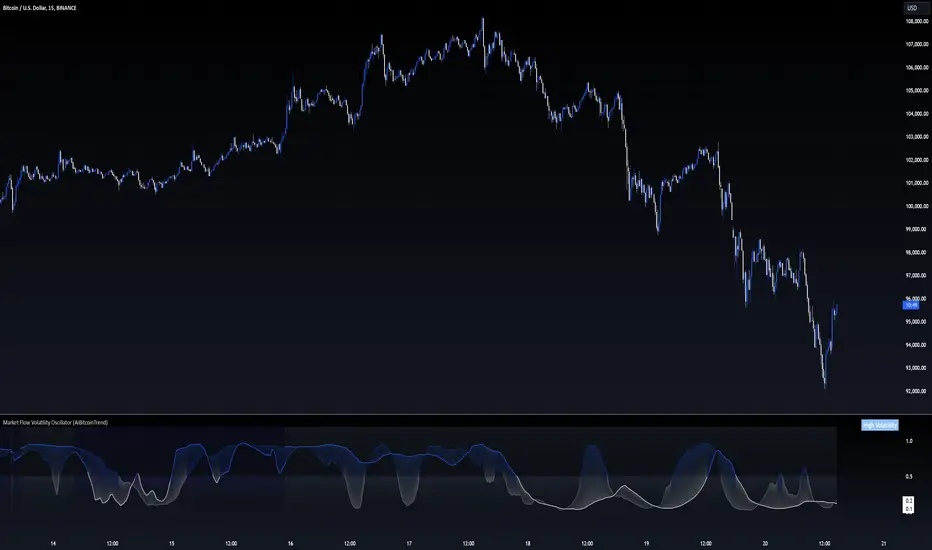
Market Flow Volatility Oscillator (AiBitcoinTrend)The Market Flow Volatility Oscillator (AiBitcoinTrend) is a cutting-edge technical analysis tool designed to evaluate and classify market volatility regimes. By leveraging Gaussian filtering and clustering techniques, this indicator provides traders with clear insights into periods of high and low volatility, helping them adapt their strategies to evolving market conditions. Built for precision and clarity, it combines advanced mathematical models with intuitive visual feedback to identify trends and volatility shifts effectively.
👽 How the Indicator Works
👾 Volatility Classification with Gaussian Filtering
The indicator detects volatility levels by applying Gaussian filters to the price series. Gaussian filters smooth out noise while preserving significant price movements. Traders can adjust the smoothing levels using sigma parameters, enabling greater flexibility:
Low Sigma: Emphasizes short-term volatility.
High Sigma: Captures broader trends with reduced sensitivity to small fluctuations.
👾 Clustering Algorithm for Regime Detection
The core of this indicator is its clustering model, which classifies market conditions into two distinct regimes:
Low Volatility Regime: Calm periods with reduced market activity.
High Volatility Regime: Intense periods with heightened price movements.
The clustering process works as follows:
A rolling window of data is analyzed to calculate the standard deviation of price returns.
Two cluster centers are initialized using the 25th and 75th percentiles of the data distribution.
Each price volatility value is assigned to the nearest cluster based on its distance to the centers.
The cluster centers are refined iteratively, providing an accurate and adaptive classification.
👾 Oscillator Generation with Slope R-Values
The indicator computes Gaussian filter slopes to generate oscillators that visualize trends:
Oscillator Low: Captures low-frequency market behavior.
Oscillator High: Tracks high-frequency, faster-changing trends.
The slope is measured using the R-value of the linear regression fit, scaled and adjusted for easier interpretation.
👽 Applications
👾 Trend Trading
When the oscillator rises above 0.5, it signals potential bullish momentum, while dips below 0.5 suggest bearish sentiment.
👾 Pullback Detection
When the oscillator peaks, especially in overbought or oversold zones, provide early warnings of potential reversals.
👽 Indicator Settings
👾 Oscillator Settings
Sigma Low/High: Controls the smoothness of the oscillators.
Smaller Values: React faster to price changes but introduce more noise.
Larger Values: Provide smoother signals with longer-term insights.
👾 Window Size and Refit Interval
Window Size: Defines the rolling period for cluster and volatility calculations.
Shorter windows: adapt faster to market changes.
Longer windows: produce stable, reliable classifications.
Disclaimer: This information is for entertainment purposes only and does not constitute financial advice. Please consult with a qualified financial advisor before making any investment decisions.
Ensemble Alerts█ OVERVIEW
This indicator creates highly customizable alert conditions and messages by combining several technical conditions into groups , which users can specify directly from the "Settings/Inputs" tab. It offers a flexible framework for building and testing complex alert conditions without requiring code modifications for each adjustment.
█ CONCEPTS
Ensemble analysis
Ensemble analysis is a form of data analysis that combines several "weaker" models to produce a potentially more robust model. In a trading context, one of the most prevalent forms of ensemble analysis is the aggregation (grouping) of several indicators to derive market insights and reinforce trading decisions. With this analysis, traders typically inspect multiple indicators, signaling trade actions when specific conditions or groups of conditions align.
Simplifying ensemble creation
Combining indicators into one or more ensembles can be challenging, especially for users without programming knowledge. It usually involves writing custom scripts to aggregate the indicators and trigger trading alerts based on the confluence of specific conditions. Making such scripts customizable via inputs poses an additional challenge, as it often involves complicated input menus and conditional logic.
This indicator addresses these challenges by providing a simple, flexible input menu where users can easily define alert criteria by listing groups of conditions from various technical indicators in simple text boxes . With this script, you can create complex alert conditions intuitively from the "Settings/Inputs" tab without ever writing or modifying a single line of code. This framework makes advanced alert setups more accessible to non-coders. Additionally, it can help Pine programmers save time and effort when testing various condition combinations.
█ FEATURES
Configurable alert direction
The "Direction" dropdown at the top of the "Settings/Inputs" tab specifies the allowed direction for the alert conditions. There are four possible options:
• Up only : The indicator only evaluates upward conditions.
• Down only : The indicator only evaluates downward conditions.
• Up and down (default): The indicator evaluates upward and downward conditions, creating alert triggers for both.
• Alternating : The indicator prevents alert triggers for consecutive conditions in the same direction. An upward condition must be the first occurrence after a downward condition to trigger an alert, and vice versa for downward conditions.
Flexible condition groups
This script features six text inputs where users can define distinct condition groups (ensembles) for their alerts. An alert trigger occurs if all the conditions in at least one group occur.
Each input accepts a comma-separated list of numbers with optional spaces (e.g., "1, 4, 8"). Each listed number, from 1 to 35, corresponds to a specific individual condition. Below are the conditions that the numbers represent:
1 — RSI above/below threshold
2 — RSI below/above threshold
3 — Stoch above/below threshold
4 — Stoch below/above threshold
5 — Stoch K over/under D
6 — Stoch K under/over D
7 — AO above/below threshold
8 — AO below/above threshold
9 — AO rising/falling
10 — AO falling/rising
11 — Supertrend up/down
12 — Supertrend down/up
13 — Close above/below MA
14 — Close below/above MA
15 — Close above/below open
16 — Close below/above open
17 — Close increase/decrease
18 — Close decrease/increase
19 — Close near Donchian top/bottom (Close > (Mid + HH) / 2)
20 — Close near Donchian bottom/top (Close < (Mid + LL) / 2)
21 — New Donchian high/low
22 — New Donchian low/high
23 — Rising volume
24 — Falling volume
25 — Volume above average (Volume > SMA(Volume, 20))
26 — Volume below average (Volume < SMA(Volume, 20))
27 — High body to range ratio (Abs(Close - Open) / (High - Low) > 0.5)
28 — Low body to range ratio (Abs(Close - Open) / (High - Low) < 0.5)
29 — High relative volatility (ATR(7) > ATR(40))
30 — Low relative volatility (ATR(7) < ATR(40))
31 — External condition 1
32 — External condition 2
33 — External condition 3
34 — External condition 4
35 — External condition 5
These constituent conditions fall into three distinct categories:
• Directional pairs : The numbers 1-22 correspond to pairs of opposing upward and downward conditions. For example, if one of the inputs includes "1" in the comma-separated list, that group uses the "RSI above/below threshold" condition pair. In this case, the RSI must be above a high threshold for the group to trigger an upward alert, and the RSI must be below a defined low threshold to trigger a downward alert.
• Non-directional filters : The numbers 23-30 correspond to conditions that do not represent directional information. These conditions act as filters for both upward and downward alerts. Traders often use non-directional conditions to refine trending or mean reversion signals. For instance, if one of the input lists includes "30", that group uses the "Low relative volatility" condition. The group can trigger an upward or downward alert only if the 7-period Average True Range (ATR) is below the 40-period ATR.
• External conditions : The numbers 31-35 correspond to external conditions based on the plots from other indicators on the chart. To set these conditions, use the source inputs in the "External conditions" section near the bottom of the "Settings/Inputs" tab. The external value can represent an upward, downward, or non-directional condition based on the following logic:
▫ Any value above 0 represents an upward condition.
▫ Any value below 0 represents a downward condition.
▫ If the checkbox next to the source input is selected, the condition becomes non-directional . Any group that uses the condition can trigger upward or downward alerts only if the source value is not 0.
To learn more about using plotted values from other indicators, see this article in our Help Center and the Source input section of our Pine Script™ User Manual.
Group markers
Each comma-separated list represents a distinct group , where all the listed conditions must occur to trigger an alert. This script assigns preset markers (names) to each condition group to make the active ensembles easily identifiable in the generated alert messages and labels. The markers assigned to each group use the format "M", where "M" is short for "Marker" and "x" is the group number. The titles of the inputs at the top of the "Settings/Inputs" tab show these markers for convenience.
For upward conditions, the labels and alert messages show group markers with upward triangles (e.g., "M1▲"). For downward conditions, they show markers with downward triangles (e.g., "M1▼").
NOTE: By default, this script populates the "M1" field with a pre-configured list for a mean reversion group ("2,18,24,28"). The other fields are empty. If any "M*" input does not contain a value, the indicator ignores it in the alert calculations.
Custom alert messages
By default, the indicator's alert message text contains the activated markers and their direction as a comma-separated list. Users can override this message for upward or downward alerts with the two text fields at the bottom of the "Settings/Inputs" tab. When the fields are not empty , the alerts use that text instead of the default marker list.
NOTE: This script generates alert triggers, not the alerts themselves. To set up an alert based on this script's conditions, open the "Create Alert" dialog box, then select the "Ensemble Alerts" and "Any alert() function call" options in the "Condition" tabs. See the Alerts FAQ in our Pine Script™ User Manual for more information.
Condition visualization
This script offers organized visualizations of its conditions, allowing users to inspect the behaviors of each condition alongside the specified groups. The key visual features include:
1) Conditional plots
• The indicator plots the history of each individual condition, excluding the external conditions, as circles at different levels. Opposite conditions appear at positive and negative levels with the same absolute value. The plots for each condition show values only on the bars where they occur.
• Each condition's plot is color-coded based on its type. Aqua and orange plots represent opposing directional conditions, and purple plots represent non-directional conditions. The titles of the plots also contain the condition numbers to which they apply.
• The plots in the separate pane can be turned on or off with the "Show plots in pane" checkbox near the top of the "Settings/Inputs" tab. This input only toggles the color-coded circles, which reduces the graphical load. If you deactivate these visuals, you can still inspect each condition from the script's status line and the Data Window.
• As a bonus, the indicator includes "Up alert" and "Down alert" plots in the Data Window, representing the combined upward and downward ensemble alert conditions. These plots are also usable in additional indicator-on-indicator calculations.
2) Dynamic labels
• The indicator draws a label on the main chart pane displaying the activated group markers (e.g., "M1▲") each time an alert condition occurs.
• The labels for upward alerts appear below chart bars. The labels for downward alerts appear above the bars.
NOTE: This indicator can display up to 500 labels because that is the maximum allowed for a single Pine script.
3) Background highlighting
• The indicator can highlight the main chart's background on bars where upward or downward condition groups activate. Use the "Highlight background" inputs in the "Settings/Inputs" tab to enable these highlights and customize their colors.
• Unlike the dynamic labels, these background highlights are available for all chart bars, irrespective of the number of condition occurrences.
█ NOTES
• This script uses Pine Script™ v6, the latest version of TradingView's programming language. See the Release notes and Migration guide to learn what's new in v6 and how to convert your scripts to this version.
• This script imports our new Alerts library, which features functions that provide high-level simplicity for working with complex compound conditions and alerts. We used the library's `compoundAlertMessage()` function in this indicator. It evaluates items from "bool" arrays in groups specified by an array of strings containing comma-separated index lists , returning a tuple of "string" values containing the marker of each activated group.
• The script imports the latest version of the ta library to calculate several technical indicators not included in the built-in `ta.*` namespace, including Double Exponential Moving Average (DEMA), Triple Exponential Moving Average (TEMA), Fractal Adaptive Moving Average (FRAMA), Tilson T3, Awesome Oscillator (AO), Full Stochastic (%K and %D), SuperTrend, and Donchian Channels.
• The script uses the `force_overlay` parameter in the label.new() and bgcolor() calls to display the drawings and background colors in the main chart pane.
• The plots and hlines use the available `display.*` constants to determine whether the visuals appear in the separate pane.
Look first. Then leap.

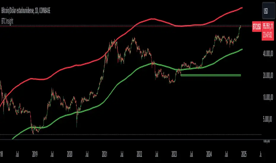
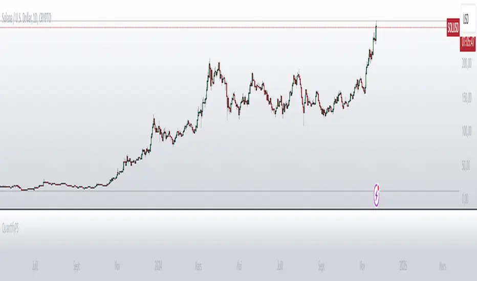
BTC InsightThis script is a comprehensive tool for analyzing Bitcoin's daily price range, trend predictions, and significant volume-based order block levels. It combines multiple technical analysis concepts, including exponential moving averages (EMAs), logarithmic calculations, and custom indicators for advanced forecasting and visualization.
Key Features and Technical Details
1. Exponential Moving Averages (EMAs)
The script calculates two smoothed EMAs:
EMA1 and EMA2 are derived from the logarithmic price of Bitcoin (log(close)).
The smoothing periods and multipliers are user-configurable through inputs:
Smoothed EMA1 Period (default: 728)
Smoothed EMA2 Period (default: 728)
Initial EMA Multipliers (default: 1.0 for EMA1, 5.0 for EMA2)
A time decay factor is applied to the multipliers to adjust sensitivity over time, making the EMAs adaptive to market dynamics.
2. Logarithmic Domain Calculations
The script uses logarithmic transformations to enhance accuracy when dealing with large price changes.
Adjustments to EMAs are made in the logarithmic domain and converted back to the price domain for plotting.
3. EMA Forecasting
The script performs a linear regression analysis over a specified period (728 bars by default) to estimate future price trends for both EMAs.
Slope Adjustments:
RSI (Relative Strength Index) is incorporated to modify the forecast slope dynamically:
RSI > 70: Bearish adjustment (-0.5)
RSI < 30: Bullish adjustment (+0.5)
Forecasts are plotted as dashed lines, projecting future values of EMA1 (green) and EMA2 (red).
4. Order Block Detection
Detects order block levels based on high volume spikes relative to the average volume over a lookback period (default: 100 bars).
A volume multiplier (default: 1.5x) is applied to identify significant volume activity.
Two types of order blocks are identified:
Below EMA1: A price zone where significant buying occurred below EMA1.
Above EMA2: A price zone where significant selling occurred above EMA2.
Order blocks are visualized as shaded rectangles:
Green boxes represent order blocks below EMA1.
Red boxes represent order blocks above EMA2.
5. Customization Inputs
The script allows fine-tuning via the following parameters:
EMA Settings: Periods, multipliers, and time factors for both EMAs.
Volume Analysis Settings: Lookback period and volume multiplier for order block detection.
Order Block Box Settings: Height of the range as a percentage of the detected price.
6. Visualization
EMAs: Two smoothed exponential moving averages are plotted with configurable offsets.
Forecast Lines: Dashed lines project future EMA trends based on regression analysis.
Order Block Boxes: Highlight areas of high volume below EMA1 and above EMA2, indicating potential support or resistance zones.
How It Works in Practice
EMAs and Trend Analysis:
The EMAs represent long-term market trends, adjusted dynamically using custom multipliers and time decay.
The script forecasts the EMAs' future trajectories to anticipate potential price movements.
Order Blocks:
High-volume zones indicate areas where significant market activity occurred, providing insights into potential price reversal points or continuation zones.
RSI Integration:
RSI-based slope adjustment fine-tunes the EMA forecast, adding an extra layer of dynamic market context.
Comprehensive View:
By combining trend forecasts with volume-based zones, the script delivers a robust analysis tool for identifying potential entry/exit points, support/resistance levels, and long-term trend predictions.
QuantifyPS - 1Library "QuantifyPS"
normdist(z)
Parameters:
z (float) : (float): The z-score for which the CDF is to be calculated.
Returns: (float): The cumulative probability corresponding to the input z-score.
Notes:
- Uses an approximation method for the normal distribution CDF, which is computationally efficient.
- The result is accurate for most practical purposes but may have minor deviations for extreme values of `z`.
Formula:
- Based on the approximation formula:
`Φ(z) ≈ 1 - f(z) * P(t)` if `z > 0`, otherwise `Φ(z) ≈ f(z) * P(t)`,
where:
`f(z) = 0.3989423 * exp(-z^2 / 2)` (PDF of standard normal distribution)
`P(t) = Σ [c * t^i]` with constants `c` and `t = 1 / (1 + 0.2316419 * |z|)`.
Implementation details:
- The approximation uses five coefficients for the polynomial part of the CDF.
- Handles both positive and negative values of `z` symmetrically.
Constants:
- The coefficients and scaling factors are chosen to minimize approximation errors.
gamma(x)
Parameters:
x (float) : (float): The input value for which the Gamma function is to be calculated.
Must be greater than 0. For x <= 0, the function returns `na` as it is undefined.
Returns: (float): Approximation of the Gamma function for the input `x`.
Notes:
- The Lanczos approximation provides a numerically stable and efficient method to compute the Gamma function.
- The function is not defined for `x <= 0` and will return `na` in such cases.
- Uses precomputed Lanczos coefficients for accuracy.
- Includes handling for small numerical inaccuracies.
Formula:
- The Gamma function is approximated as:
`Γ(x) ≈ sqrt(2π) * t^(x + 0.5) * e^(-t) * Σ(p / (x + k))`
where `t = x + g + 0.5` and `p` is the array of Lanczos coefficients.
Implementation details:
- Lanczos coefficients (`p`) are precomputed and stored in an array.
- The summation iterates over these coefficients to compute the final result.
- The constant `g` controls the precision of the approximation (commonly `g = 7`).
t_cdf(t, df)
Parameters:
t (float) : (float): The t-statistic for which the CDF value is to be calculated.
df (int) : (int): Degrees of freedom of the t-distribution.
Returns: (float): Approximate CDF value for the given t-statistic.
Notes:
- This function computes a one-tailed p-value.
- Relies on an approximation formula using gamma functions and standard t-distribution properties.
- May not be as accurate as specialized statistical libraries for extreme values or very high degrees of freedom.
Formula:
- Let `x = df / (t^2 + df)`.
- The approximation formula is derived using:
`CDF(t, df) ≈ 1 - * x^((df + 1) / 2) / 2`,
where Γ represents the gamma function.
Implementation details:
- Computes the gamma ratio for normalization.
- Applies the t-distribution formula for one-tailed probabilities.
tStatForPValue(p, df)
Parameters:
p (float) : (float): P-value for which the t-statistic needs to be calculated.
Must be in the interval (0, 1).
df (int) : (int): Degrees of freedom of the t-distribution.
Returns: (float): The t-statistic corresponding to the given p-value.
Notes:
- If `p` is outside the interval (0, 1), the function returns `na` as an error.
- The function uses binary search with a fixed number of iterations and a defined tolerance.
- The result is accurate to within the specified tolerance (default: 0.0001).
- Relies on the cumulative density function (CDF) `t_cdf` for the t-distribution.
Formula:
- Uses the cumulative density function (CDF) of the t-distribution to iteratively find the t-statistic.
Implementation details:
- `low` and `high` define the search interval for the t-statistic.
- The midpoint (`mid`) is iteratively refined until the difference between the cumulative probability
and the target p-value is smaller than the tolerance.
jarqueBera(n, s, k)
Parameters:
n (float) : (series float): Number of observations in the dataset.
s (float) : (series float): Skewness of the dataset.
k (float) : (series float): Kurtosis of the dataset.
Returns: (float): The Jarque-Bera test statistic.
Formula:
JB = n *
Notes:
- A higher JB value suggests that the data deviates more from a normal distribution.
- The test is asymptotically distributed as a chi-squared distribution with 2 degrees of freedom.
- Use this value to calculate a p-value to determine the significance of the result.
skewness(data)
Parameters:
data (float) : (series float): Input data series.
Returns: (float): The skewness value.
Notes:
- Handles missing values (`na`) by ignoring invalid points.
- Includes error handling for zero variance to avoid division-by-zero scenarios.
- Skewness is calculated as the normalized third central moment of the data.
kurtosis(data)
Parameters:
data (float) : (series float): Input data series.
Returns: (float): The kurtosis value.
Notes:
- Handles missing values (`na`) by ignoring invalid points.
- Includes error handling for zero variance to avoid division-by-zero scenarios.
- Kurtosis is calculated as the normalized fourth central moment of the data.
regression(y, x, lag)
Parameters:
y (float) : (series float): Dependent series (observed values).
x (float) : (series float): Independent series (explanatory variable).
lag (int) : (int): Number of lags applied to the independent series (x).
Returns: (tuple): Returns a tuple containing the following values:
- n: Number of valid observations.
- alpha: Intercept of the regression line.
- beta: Slope of the regression line.
- t_stat: T-statistic for the beta coefficient.
- p_value: Two-tailed p-value for the beta coefficient.
- r_squared: Coefficient of determination (R²) indicating goodness of fit.
- skew: Skewness of the residuals.
- kurt: Kurtosis of the residuals.
Notes:
- Handles missing data (`na`) by ignoring invalid points.
- Includes basic error handling for zero variance and division-by-zero scenarios.
- Computes residual-based statistics (skewness and kurtosis) for model diagnostics.
STRATEGY Fibonacci Levels with High/Low Criteria - AYNET
Here is an explanation of the Fibonacci Levels Strategy with High/Low Criteria script:
Overview
This strategy combines Fibonacci retracement levels with high/low criteria to generate buy and sell signals based on price crossing specific thresholds. It utilizes higher timeframe (HTF) candlesticks and user-defined lookback periods for high/low levels.
Key Features
Higher Timeframe Integration:
The script calculates the open, high, low, and close values of the higher timeframe (HTF) candlestick.
Users can choose to calculate levels based on the current or the last HTF candle.
Fibonacci Levels:
Fibonacci retracement levels are dynamically calculated based on the HTF candlestick's range (high - low).
Users can customize the levels (0.000, 0.236, 0.382, 0.500, 0.618, 0.786, 1.000).
High/Low Lookback Criteria:
The script evaluates the highest high and lowest low over user-defined lookback periods.
These levels are plotted on the chart for visual reference.
Trade Signals:
Long Signal: Triggered when the close price crosses above both:
The lowest price criteria (lookback period).
The Fibonacci level 3 (default: 0.5).
Short Signal: Triggered when the close price crosses below both:
The highest price criteria (lookback period).
The Fibonacci level 3 (default: 0.5).
Visualization:
Plots Fibonacci levels and high/low criteria on the chart for easy interpretation.
Inputs
Higher Timeframe:
Users can select the timeframe (default: Daily) for the HTF candlestick.
Option to calculate based on the current or last HTF candle.
Lookback Periods:
lowestLookback: Number of bars for the lowest low calculation (default: 20).
highestLookback: Number of bars for the highest high calculation (default: 10).
Fibonacci Levels:
Fully customizable Fibonacci levels ranging from 0.000 to 1.000.
Visualization
Fibonacci Levels:
Plots six customizable Fibonacci levels with distinct colors and transparency.
High/Low Criteria:
Plots the highest and lowest levels based on the lookback periods as reference lines.
Trading Logic
Long Condition:
Price must close above:
The lowest price criteria (lowcriteria).
The Fibonacci level 3 (50% retracement).
Short Condition:
Price must close below:
The highest price criteria (highcriteria).
The Fibonacci level 3 (50% retracement).
Use Case
Trend Reversal Strategy:
Combines Fibonacci retracement with recent high/low criteria to identify potential reversal or breakout points.
Custom Timeframe Analysis:
Incorporates higher timeframe data for multi-timeframe trading strategies.

Exposure Oscillator (Cumulative 0 to ±100%)
Exposure Oscillator (Cumulative 0 to ±100%)
This Pine Script indicator plots an "Exposure Oscillator" on the chart, which tracks the cumulative market exposure from a range of technical buy and sell signals. The exposure is measured on a scale from -100% (maximum short exposure) to +100% (maximum long exposure), helping traders assess the strength of their position in the market. It provides an intuitive visual cue to aid decision-making for trend-following strategies.
Buy Signals (Increase Exposure Score by +10%)
Buy Signal 1 (Cross Above 21 EMA):
This signal is triggered when the price crosses above the 21-period Exponential Moving Average (EMA), where the current bar closes above the EMA21, and the previous bar closed below the EMA21. This indicates a potential upward price movement as the market shifts into a bullish trend.
buySignal1 = ta.crossover(close, ema21)
Buy Signal 2 (Trending Above 21 EMA):
This signal is triggered when the price closes above the 21-period EMA for each of the last 5 bars, indicating a sustained bullish trend. It confirms that the price is consistently above the EMA21 for a significant period.
buySignal2 = ta.barssince(close <= ema21) > 5
Buy Signal 3 (Living Above 21 EMA):
This signal is triggered when the price has closed above the 21-period EMA for each of the last 15 bars, demonstrating a strong, prolonged uptrend.
buySignal3 = ta.barssince(close <= ema21) > 15
Buy Signal 4 (Cross Above 50 SMA):
This signal is triggered when the price crosses above the 50-period Simple Moving Average (SMA), where the current bar closes above the 50 SMA, and the previous bar closed below it. It indicates a shift toward bullish momentum.
buySignal4 = ta.crossover(close, sma50)
Buy Signal 5 (Cross Above 200 SMA):
This signal is triggered when the price crosses above the 200-period Simple Moving Average (SMA), where the current bar closes above the 200 SMA, and the previous bar closed below it. This suggests a long-term bullish trend.
buySignal5 = ta.crossover(close, sma200)
Buy Signal 6 (Low Above 50 SMA):
This signal is true when the lowest price of the current bar is above the 50-period SMA, indicating strong bullish pressure as the price maintains itself above the moving average.
buySignal6 = low > sma50
Buy Signal 7 (Accumulation Day):
An accumulation day occurs when the closing price is in the upper half of the daily range (greater than 50%) and the volume is larger than the previous bar's volume, suggesting buying pressure and accumulation.
buySignal7 = (close - low) / (high - low) > 0.5 and volume > volume
Buy Signal 8 (Higher High):
This signal occurs when the current bar’s high exceeds the highest high of the previous 14 bars, indicating a breakout or strong upward momentum.
buySignal8 = high > ta.highest(high, 14)
Buy Signal 9 (Key Reversal Bar):
This signal is generated when the stock opens below the low of the previous bar but rallies to close above the previous bar’s high, signaling a potential reversal from bearish to bullish.
buySignal9 = open < low and close > high
Buy Signal 10 (Distribution Day Fall Off):
This signal is triggered when a distribution day (a day with high volume and a close near the low of the range) "falls off" the rolling 25-bar period, indicating the end of a bearish trend or selling pressure.
buySignal10 = ta.barssince(close < sma50 and close < sma50) > 25
Sell Signals (Decrease Exposure Score by -10%)
Sell Signal 1 (Cross Below 21 EMA):
This signal is triggered when the price crosses below the 21-period Exponential Moving Average (EMA), where the current bar closes below the EMA21, and the previous bar closed above it. It suggests that the market may be shifting from a bullish trend to a bearish trend.
sellSignal1 = ta.crossunder(close, ema21)
Sell Signal 2 (Trending Below 21 EMA):
This signal is triggered when the price closes below the 21-period EMA for each of the last 5 bars, indicating a sustained bearish trend.
sellSignal2 = ta.barssince(close >= ema21) > 5
Sell Signal 3 (Living Below 21 EMA):
This signal is triggered when the price has closed below the 21-period EMA for each of the last 15 bars, suggesting a strong downtrend.
sellSignal3 = ta.barssince(close >= ema21) > 15
Sell Signal 4 (Cross Below 50 SMA):
This signal is triggered when the price crosses below the 50-period Simple Moving Average (SMA), where the current bar closes below the 50 SMA, and the previous bar closed above it. It indicates the start of a bearish trend.
sellSignal4 = ta.crossunder(close, sma50)
Sell Signal 5 (Cross Below 200 SMA):
This signal is triggered when the price crosses below the 200-period Simple Moving Average (SMA), where the current bar closes below the 200 SMA, and the previous bar closed above it. It indicates a long-term bearish trend.
sellSignal5 = ta.crossunder(close, sma200)
Sell Signal 6 (High Below 50 SMA):
This signal is true when the highest price of the current bar is below the 50-period SMA, indicating weak bullishness or a potential bearish reversal.
sellSignal6 = high < sma50
Sell Signal 7 (Distribution Day):
A distribution day is identified when the closing range of a bar is less than 50% and the volume is larger than the previous bar's volume, suggesting that selling pressure is increasing.
sellSignal7 = (close - low) / (high - low) < 0.5 and volume > volume
Sell Signal 8 (Lower Low):
This signal occurs when the current bar's low is less than the lowest low of the previous 14 bars, indicating a breakdown or strong downward momentum.
sellSignal8 = low < ta.lowest(low, 14)
Sell Signal 9 (Downside Reversal Bar):
A downside reversal bar occurs when the stock opens above the previous bar's high but falls to close below the previous bar’s low, signaling a reversal from bullish to bearish.
sellSignal9 = open > high and close < low
Sell Signal 10 (Distribution Cluster):
This signal is triggered when a distribution day occurs three times in the rolling 7-bar period, indicating significant selling pressure.
sellSignal10 = ta.valuewhen((close < low) and volume > volume , 1, 7) >= 3
Theme Mode:
Users can select the theme mode (Auto, Dark, or Light) to match the chart's background or to manually choose a light or dark theme for the oscillator's appearance.
Exposure Score Calculation: The script calculates a cumulative exposure score based on a series of buy and sell signals.
Buy signals increase the exposure score, while sell signals decrease it. Each signal impacts the score by ±10%.
Signal Conditions: The buy and sell signals are derived from multiple conditions, including crossovers with moving averages (EMA21, SMA50, SMA200), trend behavior, and price/volume analysis.
Oscillator Visualization: The exposure score is visualized as a line on the chart, changing color based on whether the exposure is positive (long position) or negative (short position). It is limited to the range of -100% to +100%.
Position Type: The indicator also indicates the position type based on the exposure score, labeling it as "Long," "Short," or "Neutral."
Horizontal Lines: Reference lines at 0%, 100%, and -100% visually mark neutral, increasing long, and increasing short exposure levels.
Exposure Table: A table displays the current exposure level (in percentage) and position type ("Long," "Short," or "Neutral"), updated dynamically based on the oscillator’s value.
Inputs:
Theme Mode: Choose "Auto" to use the default chart theme, or manually select "Dark" or "Light."
Usage:
This oscillator is designed to help traders track market sentiment, gauge exposure levels, and manage risk. It can be used for long-term trend-following strategies or short-term trades based on moving average crossovers and volume analysis.
The oscillator operates in conjunction with the chart’s price action and provides a visual representation of the market’s current trend strength and exposure.
Important Considerations:
Risk Management: While the exposure score provides valuable insight, it should be combined with other risk management tools and analysis for optimal trading decisions.
Signal Sensitivity: The accuracy and effectiveness of the signals depend on market conditions and may require adjustments based on the user’s trading strategy or timeframe.
Disclaimer:
This script is for educational purposes only. Trading involves significant risk, and users should carefully evaluate all market conditions and apply appropriate risk management strategies before using this tool in live trading environments.

Uptrick: DPO Signal & Zone Indicator
## **Uptrick: DPO Signal & Zone Indicator**
### **Introduction:**
The **Uptrick: DPO Signal & Zone Indicator** is a sophisticated technical analysis tool tailored to provide insights into market momentum, identify potential trading signals, and recognize extreme market conditions. It leverages the Detrended Price Oscillator (DPO) to strip out long-term trends from price movements, allowing traders to focus on short-term fluctuations and cyclical behavior. The indicator integrates multiple components, including a Detrended Price Oscillator, a Signal Line, a Histogram, and customizable alert levels, to deliver a robust framework for market analysis and trading decision-making.
### **Detailed Breakdown:**
#### **1. Detrended Price Oscillator (DPO):**
- **Purpose and Functionality:**
- The DPO is designed to filter out long-term trends from the price data, isolating short-term price movements. This helps in understanding the cyclical patterns and momentum of an asset, allowing traders to detect periods of acceleration or deceleration that might be overlooked when focusing solely on long-term trends.
- **Calculation:**
- **Formula:** `dpo = close - ta.sma(close, smaLength)`
- **`close`:** The asset’s closing price for each period in the dataset.
- **`ta.sma(close, smaLength)`:** The Simple Moving Average (SMA) of the closing prices over a period defined by `smaLength`.
- The DPO is derived by subtracting the SMA value from the current closing price. This calculation reveals how much the current price deviates from the moving average, effectively detrending the price data.
- **Interpretation:**
- **Positive DPO Values:** Indicate that the current price is higher than the moving average, suggesting bullish market conditions and a potential upward trend.
- **Negative DPO Values:** Indicate that the current price is lower than the moving average, suggesting bearish market conditions and a potential downward trend.
- **Magnitude of DPO:** Reflects the strength of momentum. Larger positive or negative values suggest stronger momentum in the respective direction.
#### **2. Signal Line:**
- **Purpose and Functionality:**
- The Signal Line is a smoothed average of the DPO, intended to act as a reference point for generating trading signals. It helps to filter out short-term fluctuations and provides a clearer perspective on the prevailing trend.
- **Calculation:**
- **Formula:** `signalLine = ta.sma(dpo, signalLength)`
- **`ta.sma(dpo, signalLength)`:** The SMA of the DPO values over a period defined by `signalLength`.
- The Signal Line is calculated by applying a moving average to the DPO values. This smoothing process reduces noise and highlights the underlying trend direction.
- **Interpretation:**
- **DPO Crossing Above Signal Line:** Generates a buy signal, suggesting that short-term momentum is turning bullish relative to the longer-term trend.
- **DPO Crossing Below Signal Line:** Generates a sell signal, suggesting that short-term momentum is turning bearish relative to the longer-term trend.
- **Signal Line’s Role:** Provides a benchmark for assessing the strength of the DPO. The interaction between the DPO and the Signal Line offers actionable insights into potential entry or exit points.
#### **3. Histogram:**
- **Purpose and Functionality:**
- The Histogram visualizes the difference between the DPO and the Signal Line. It provides a graphical representation of momentum strength and direction, allowing traders to quickly gauge market conditions.
- **Calculation:**
- **Formula:** `histogram = dpo - signalLine`
- The Histogram is computed by subtracting the Signal Line value from the DPO value. Positive values indicate that the DPO is above the Signal Line, while negative values indicate that the DPO is below the Signal Line.
- **Interpretation:**
- **Color Coding:**
- **Green Bars:** Represent positive values, indicating bullish momentum.
- **Red Bars:** Represent negative values, indicating bearish momentum.
- **Width of Bars:** Indicates the strength of momentum. Wider bars signify stronger momentum, while narrower bars suggest weaker momentum.
- **Zero Line:** A horizontal gray line that separates positive and negative histogram values. Crosses of the histogram through this zero line can signal shifts in momentum direction.
#### **4. Alert Levels:**
- **Purpose and Functionality:**
- Alert levels define specific thresholds to identify extreme market conditions, such as overbought and oversold states. These levels help traders recognize potential reversal points and extreme market conditions.
- **Inputs:**
- **`alertLevel1`:** Defines the upper threshold for identifying overbought conditions.
- **Default Value:** 0.5
- **`alertLevel2`:** Defines the lower threshold for identifying oversold conditions.
- **Default Value:** -0.5
- **Interpretation:**
- **Overbought Condition:** When the DPO exceeds `alertLevel1`, indicating that the market may be overbought. This condition suggests that the asset could be due for a correction or reversal.
- **Oversold Condition:** When the DPO falls below `alertLevel2`, indicating that the market may be oversold. This condition suggests that the asset could be poised for a rebound or reversal.
#### **5. Visual Elements:**
- **DPO and Signal Line Plots:**
- **DPO Plot:**
- **Color:** Blue
- **Width:** 2 pixels
- **Purpose:** To visually represent the deviation of the current price from the moving average.
- **Signal Line Plot:**
- **Color:** Red
- **Width:** 1 pixel
- **Purpose:** To provide a smoothed reference for the DPO and generate trading signals.
- **Histogram Plot:**
- **Color Coding:**
- **Green:** For positive values, signaling bullish momentum.
- **Red:** For negative values, signaling bearish momentum.
- **Style:** Histogram bars are displayed with varying width to represent the strength of momentum.
- **Zero Line:** A gray horizontal line separating positive and negative histogram values.
- **Overbought/Oversold Zones:**
- **Background Colors:**
- **Green Shading:** Applied when the DPO exceeds `alertLevel1`, indicating an overbought condition.
- **Red Shading:** Applied when the DPO falls below `alertLevel2`, indicating an oversold condition.
- **Horizontal Lines:**
- **Dotted Green Line:** At `alertLevel1`, marking the upper alert threshold.
- **Dotted Red Line:** At `alertLevel2`, marking the lower alert threshold.
- **Purpose:** To provide clear visual cues for extreme market conditions, aiding in the identification of potential reversal points.
#### **6. Trading Signals and Alerts:**
- **Buy Signal:**
- **Trigger:** When the DPO crosses above the Signal Line.
- **Visual Representation:** A "BUY" label appears below the price bar in the specified buy color.
- **Purpose:** Indicates a potential buying opportunity as short-term momentum turns bullish.
- **Sell Signal:**
- **Trigger:** When the DPO crosses below the Signal Line.
- **Visual Representation:** A "SELL" label appears above the price bar in the specified sell color.
- **Purpose:** Indicates a potential selling opportunity as short-term momentum turns bearish.
- **Overbought/Oversold Alerts:**
- **Overbought Alert:** Triggered when the DPO crosses below `alertLevel1`.
- **Oversold Alert:** Triggered when the DPO crosses above `alertLevel2`.
- **Visual Representation:** Labels "OVERBOUGHT" and "OVERSOLD" appear with distinctive colors and sizes to highlight extreme conditions.
- **Purpose:** To signal potential reversal points and extreme market conditions that may lead to price corrections or trend reversals.
- **Alert Conditions:**
- **DPO Cross Above Signal Line:** Alerts traders when the DPO crosses above the Signal Line, generating a buy signal.
- **DPO Cross Below Signal Line:** Alerts traders when the DPO crosses below the Signal Line, generating a sell signal.
- **DPO Above Upper Alert Level:** Alerts when the DPO is above `alertLevel1`, indicating an overbought condition.
- **DPO Below Lower Alert Level:** Alerts when the DPO is below `alertLevel2`, indicating an oversold condition.
- **Purpose:** To provide real-time notifications of significant market events, enabling traders to make informed decisions promptly.
### **Practical Applications:**
#### **1. Trend Following Strategies:**
- **Objective:**
- To capture and ride the prevailing market trends by entering trades that align with the direction of the momentum.
- **How to Use:**
- Monitor buy and sell signals generated by the DPO crossing the Signal Line. A buy signal suggests a bullish trend and a potential long trade, while a sell signal suggests a bearish trend and a potential short trade.
- Use the Histogram to confirm the strength of the trend. Expanding green bars indicate strong bullish momentum, while expanding red bars indicate strong bearish momentum.
- **Advantages:**
- Helps traders stay aligned with the market trend, increasing the likelihood of capturing substantial price moves.
#### **2. Reversal Trading:**
- **Objective:**
- To identify potential market reversals
by detecting overbought and oversold conditions.
- **How to Use:**
- Look for overbought and oversold signals based on the DPO crossing `alertLevel1` and `alertLevel2`. These conditions suggest that the market may be due for a reversal.
- Confirm reversal signals with the Histogram. A decrease in histogram bars (from green to red or vice versa) may support the reversal hypothesis.
- **Advantages:**
- Provides early warnings of potential market reversals, allowing traders to position themselves before significant price changes occur.
#### **3. Momentum Analysis:**
- **Objective:**
- To gauge the strength and direction of market momentum for making informed trading decisions.
- **How to Use:**
- Analyze the Histogram to assess momentum strength. Positive and expanding histogram bars indicate increasing bullish momentum, while negative and expanding bars suggest increasing bearish momentum.
- Use momentum insights to validate or question existing trading positions and strategies.
- **Advantages:**
- Offers valuable information about the market's momentum, helping traders confirm the validity of trends and trading signals.
### **Customization and Flexibility:**
The **Uptrick: DPO Signal & Zone Indicator** offers extensive customization options to accommodate diverse trading preferences and market conditions:
- **SMA Length and Signal Line Length:**
- Adjust the `smaLength` and `signalLength` parameters to control the sensitivity and responsiveness of the DPO and Signal Line. Shorter lengths make the indicator more responsive to price changes, while longer lengths provide smoother, less volatile signals.
- **Alert Levels:**
- Modify `alertLevel1` and `alertLevel2` to fit varying market conditions and volatility. Setting these levels appropriately helps tailor the indicator to different asset classes and trading strategies.
- **Color and Shape Customization:**
- Customize the colors and sizes of buy/sell signals, histogram bars, and alert levels to enhance visual clarity and align with personal preferences. This customization helps ensure that the indicator integrates seamlessly with a trader's charting setup.
### **Conclusion:**
The **Uptrick: DPO Signal & Zone Indicator** is a multifaceted analytical tool that combines the power of the Detrended Price Oscillator with customizable visual elements and alert levels to deliver a comprehensive approach to market analysis. By offering insights into momentum strength, trend direction, and potential reversal points, this indicator equips traders with valuable information to make informed decisions and enhance their trading strategies. Its flexibility and customization options ensure that it can be adapted to various trading styles and market conditions, making it a versatile addition to any trader's toolkit.

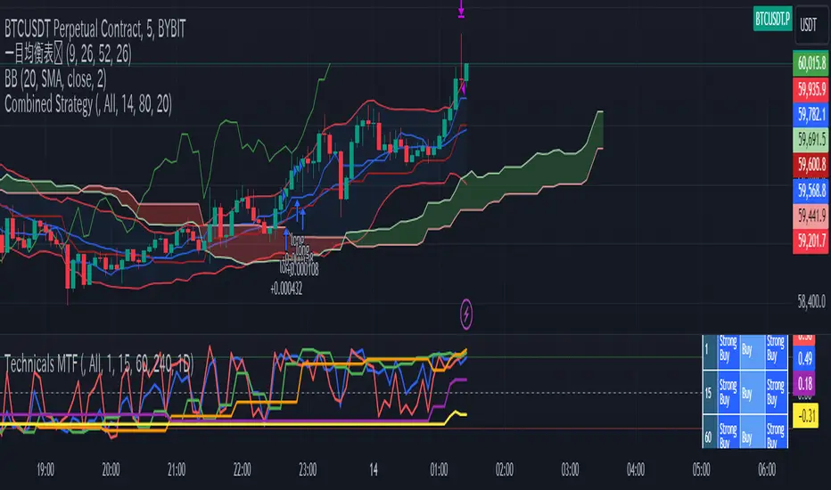
Super Technical RatingsThis indicator, titled "Super Technical Ratings," is designed to provide a multi-timeframe technical analysis based on Moving Averages (MAs) and Oscillators. It offers a comprehensive view by evaluating the strength of buy and sell signals across multiple timeframes, displaying these evaluations both visually on the chart and in a table format.
I know that Technical Ratings is one of the most excellent indicators, but it’s also true that trends can often be misread due to the influence of other timeframes. Especially on shorter timeframes, there can be sudden price movements influenced by trends in longer timeframes. While it’s important to check other timeframes, switching between charts can be very cumbersome. I created this indicator with the hope of being able to check the Technical Ratings across multiple timeframes on a single screen. It goes without saying, I recommend displaying it as lines rather than histograms.
Key Features:
1. **Multi-Timeframe Analysis:**
- The indicator evaluates technical ratings on five different timeframes: 60 minutes, 240 minutes, 1 day, 1 week, and 1 month.
- Each timeframe is individually analyzed using a combination of Moving Averages and Oscillators, or either one depending on the user’s settings.
2. **Technical Ratings Calculation:**
- The ratings are based on the overall combination of MAs and Oscillators (`All`), MAs only, or Oscillators only, depending on the user's selection.
- The rating results are categorized into five statuses: "Strong Buy," "Buy," "Neutral," "Sell," and "Strong Sell."
3. **Table Display:**
- A table is generated on the chart to show the technical ratings for each timeframe. The table columns display the timeframe and the corresponding ratings for MAs, Oscillators, and their combination.
- The table cells are color-coded based on the rating, making it easy to quickly identify strong buy or sell signals.
4. **Graphical Plotting:**
- The indicator plots the technical rating signals for each timeframe on the chart. Different colors are used for each timeframe to help distinguish between them.
- Horizontal lines are plotted at 0, +0.5, and -0.5 levels to indicate key thresholds, making it easier to interpret the strength of the signals.
5. **Alert Conditions:**
- The indicator can trigger alerts when the technical rating crosses certain thresholds (e.g., moving from a neutral rating to a buy or sell rating).
- This helps users stay informed of significant changes in the market conditions.
Use Case:
This indicator is particularly useful for traders who want to see a consolidated view of technical ratings across multiple timeframes. It allows for a quick assessment of whether a security is generally considered a buy or sell across different time periods, aiding in making more informed trading decisions. The visual representation, combined with the color-coded table, provides an intuitive way to understand the current market sentiment.
Multiple Non-Linear Regression [ChartPrime]This indicator is designed to perform multiple non-linear regression analysis using four independent variables: close, open, high, and low prices. Here's a breakdown of its components and functionalities:
Inputs:
Users can adjust several parameters:
Normalization Data Length: Length of data used for normalization.
Learning Rate: Rate at which the algorithm learns from errors.
Smooth?: Option to smooth the output.
Smooth Length: Length of smoothing if enabled.
Define start coefficients: Initial coefficients for the regression equation.
Data Normalization:
The script normalizes input data to a range between 0 and 1 using the highest and lowest values within a specified length.
Non-linear Regression:
It calculates the regression equation using the input coefficients and normalized data. The equation used is a weighted sum of the independent variables, with coefficients adjusted iteratively using gradient descent to minimize errors.
Error Calculation:
The script computes the error between the actual and predicted values.
Gradient Descent: The coefficients are updated iteratively using gradient descent to minimize the error.
// Compute the predicted values using the non-linear regression function
predictedValues = nonLinearRegression(x_1, x_2, x_3, x_4, b1, b2, b3, b4)
// Compute the error
error = errorModule(initial_val, predictedValues)
// Update the coefficients using gradient descent
b1 := b1 - (learningRate * (error * x_1))
b2 := b2 - (learningRate * (error * x_2))
b3 := b3 - (learningRate * (error * x_3))
b4 := b4 - (learningRate * (error * x_4))
Visualization:
Plotting of normalized input data (close, open, high, low).
The indicator provides visualization of normalized data values (close, open, high, low) in the form of circular markers on the chart, allowing users to easily observe the relative positions of these values in relation to each other and the regression line.
Plotting of the regression line.
Color gradient on the regression line based on its value and bar colors.
Display of normalized input data and predicted value in a table.
Signals for crossovers with a midline (0.5).
Interpretation:
Users can interpret the regression line and its crossovers with the midline (0.5) as signals for potential buy or sell opportunities.
This indicator helps users analyze the relationship between multiple variables and make trading decisions based on the regression analysis. Adjusting the coefficients and parameters can fine-tune the model's performance according to specific market conditions.

Fisher ForLoop [InvestorUnknown]Overview
The Fisher ForLoop indicator is designed to apply the Fisher Transform over a range of lengths and signal modes. It calculates an array of Fisher values, averages them, and then applies an EMA to these values to derive a trend signal. This indicator can be customized with various settings to suit different trading strategies.
User Inputs
Start Length (a): The initial length for the Fisher Transform calculation (inclusive).
End Length (b): The final length for the Fisher Transform calculation (inclusive).
EMA Length (c): The length of the EMA applied to the average Fisher values.
Calculation Source (s): The price source used for calculations (e.g., ohlc4).
Signal Calculation
Signal Mode (sigmode): Determines the type of signal generated by the indicator. Options are "Fast", "Slow", "Thresholds Crossing", and "Fast Threshold".
1. Slow: is a simple crossing of the midline (0).
2. Fast: positive signal depends if the current Fisher EMA is above Fisher EMA or above 0.99, otherwise the signal is negative.
3. Thresholds Crossing: simple ta.crossover and ta.crossunder of the user defined threshold for Long and Short.
4. Fast Threshold: signal changes if the value of Fisher EMA changes by more than user defined threshold against the current signal
// Determine the color based on the EMA value
// If EMA is greater than 0, use the bullish color, otherwise use the bearish color
col1 = EMA > 0 ? colup : coldn
// Determine the color based on the EMA trend
// If the current EMA is greater than the previous EMA or greater than 0.99, use the bullish color, otherwise use the bearish color
col2 = EMA > EMA or EMA > 0.99 ? colup : coldn
// Initialize a variable for the color based on threshold crossings
var color col3 = na
// If the EMA crosses over the long threshold, set the color to bullish
if ta.crossover(EMA, longth)
col3 := colup
// If the EMA crosses under the short threshold, set the color to bearish
if ta.crossunder(EMA, shortth)
col3 := coldn
// Initialize a variable for the color based on fast threshold changes
var color col4 = na
// If the EMA increases by more than the fast threshold, set the color to bullish
if (EMA > EMA + fastth)
col4 := colup
// If the EMA decreases by more than the fast threshold, set the color to bearish
if (EMA < EMA - fastth)
col4 := coldn
// Initialize the final color variable
color col = na
// Set the color based on the selected signal mode
if sigmode == "Slow"
col := col1 // Use slow mode color
if sigmode == "Fast"
col := col2 // Use fast mode color
if sigmode == "Thresholds Crossing"
col := col3 // Use thresholds crossing color
if sigmode == "Fast Threshold"
col := col4 // Use fast threshold color
else
na // If no valid signal mode is selected, set color to na
Visualization Settings
Bull Color (colup): The color used to indicate bullish signals.
Bear Color (coldn): The color used to indicate bearish signals.
Color Bars (barcol): Option to color the bars based on the signal.
Custom Function: FisherForLoop
This function calculates an array of Fisher values over a specified range of lengths (from a to b). It then computes the average of these values and applies an EMA to derive the final trend signal.
// Function to calculate an array of Fisher values over a range of lengths
FisherForLoop(a, b, c, s) =>
// Initialize an array to store Fisher values for each length
var FisherArray = array.new_float(b - a + 1, 0.0)
// Loop through each length from 'a' to 'b'
for x = 0 to (b - a)
// Calculate the current length
len = a + x
// Calculate the highest and lowest values over the current length
high_ = ta.highest(s, len)
low_ = ta.lowest(s, len)
// Initialize the value variable
value = 0.0
// Update the value using the Fisher Transform formula
// The formula normalizes the price to a range between -0.5 and 0.5, then smooths it
value := .66 * ((s - low_) / (high_ - low_) - .5) + .67 * nz(value )
// Clamp the value to be within -0.999 to 0.999 to avoid math errors
val = value > .99 ? .999 : value < -.99 ? -.999 : value
// Initialize the fish1 variable
fish1 = 0.0
// Apply the Fisher Transform to the normalized value
// This converts the value to a Fisher value, which emphasizes extreme changes in price
fish1 := .5 * math.log((1 + val) / (1 - val)) + .5 * nz(fish1 )
// Store the previous Fisher value for comparison
fish2 = fish1
// Determine the trend based on the Fisher values
// If the current Fisher value is greater than the previous, the trend is up (1)
// Otherwise, the trend is down (-1)
trend = fish1 > fish2 ? 1 : -1
// Store the trend in the FisherArray at the current index
array.set(FisherArray, x, trend)
// Calculate the average of the FisherArray
Avg = array.avg(FisherArray)
// Apply an EMA to the average Fisher values to smooth the result
EMA = ta.ema(Avg, c)
// Return the FisherArray, the average, and the EMA
// Call the FisherForLoop function with the user-defined inputs
= FisherForLoop(a, b, c, s)
Important Considerations
Speed: This indicator is very fast and can provide rapid signals for potential entries. However, this speed also means it may generate false signals if used in isolation.
Complementary Use: It is recommended to use this indicator in conjunction with other indicators and analysis methods to confirm signals and enhance the reliability of your trading strategy.
Strength: The main strength of the Fisher ForLoop indicator is its ability to identify very fast entries and prevent entries against the current (short-term) market trend.
This indicator is useful for identifying trends and potential reversal points in the market, providing flexibility through its customizable settings. However, due to its sensitivity and speed, it should be used as part of a broader trading strategy rather than as a standalone tool.

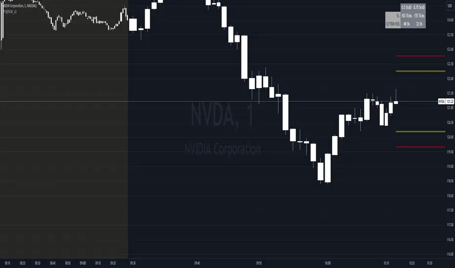
QTY@RISK VWAP based calculationVWAP Volatility-Based Risk Management Calculator for Intraday Trading
Overview
This script is an innovative tool designed to help traders manage risk effectively by calculating position sizes and stop-loss levels using the Volume Weighted Average Price (VWAP) and its standard deviation (StdDev). Unlike traditional methods that rely on time-based calculations, this approach is time-independent within the intraday timeframe, making it particularly useful for traders seeking precision and efficiency.
Key Concepts
VWAP (Volume Weighted Average Price): VWAP is a trading benchmark that represents the average price a security has traded at throughout the day, based on both volume and price. It provides insight into the average price level over a specific period, helping traders understand the market trend.
StdDev (Standard Deviation): In the context of VWAP, the standard deviation measures the volatility around the VWAP. It provides a quantifiable range that traders can use to set stop-loss levels, ensuring they are neither too tight nor too loose.
How the Script Works
1. VWAP Calculation: The script calculates the VWAP continuously as the market trades, integrating both price and volume data.
2. Volatility Measurement: It then computes the standard deviation of the VWAP, giving a measure of market volatility.
3. Stop-Loss Calculation: Using user-defined StdDev factors, the script calculates two stop-loss levels. These levels adjust dynamically based on market conditions, ensuring they remain relevant throughout the trading session.
4. Position Sizing: By incorporating your risk tolerance, the script determines the appropriate position size. This ensures that your maximum loss per trade does not exceed your predefined risk value.
How to Use the Calculator
1. Select Two VWAP StdDev Factors: Choose two standard deviation factors for calculating stop-loss levels. For example, you might choose 0.5 and 0.75 to set conservative and aggressive stop-losses respectively.
2. Set Your Trading Account Size: Enter your total trading capital. For example, $50,000.
3. Maximum Lot Size: Define the maximum number of shares you are willing to trade in a single position. For instance, 200 shares.
4. Risk Value per Trade: Input the maximum amount of money you are willing to risk on a single trade. For instance, $50.
5. Plotting Options: If you wish to visualize the stop-loss levels, enable the plot option and choose the price base for the plot, such as the closing price or the average of the high and low prices (hl2).
Example of Use
1. Initial Setup: After the market opens, wait for at least 15 minutes to ensure the VWAP has stabilized with sufficient volume data.
2. Parameter Configuration: Input your desired parameters into the calculator. For instance:
- VWAP StdDev Factors: 0.5 and 0.75
- Trading Account Size: $50,000
- Maximum Lot Size: 200 shares
- Risk Value per Trade: $50
- Plot Option: On, using "hl2" or "close" as the price base
3. Execution: Based on the inputs, the script calculates the position size and stop-loss levels. If the calculated stop-loss falls within the selected VWAP StdDev range, it will provide you with precise stop-loss prices.
4. Trading: Use the calculated position size and stop-loss levels to execute your trades confidently, knowing that your risk is managed effectively.
Advantages for Traders
- Time Independence: By relying on VWAP and its StdDev, the calculations are not dependent on specific time intervals, making them more adaptable to real-time trading conditions.
- Focus on Strategy: Novice traders can focus more on their trading strategies rather than getting bogged down with complex calculations.
- Dynamic Adjustments: The script adjusts stop-loss levels dynamically based on evolving market conditions, providing more accurate and relevant risk management.
- Flexibility: Traders can tailor the calculator to their risk preferences and trading style by adjusting the StdDev factors and risk parameters.
By incorporating these concepts and using this risk management calculator, traders can enhance their trading efficiency, improve their risk management, and ultimately make more informed trading decisions.
Adaptive Trend Lines [MAMA and FAMA]Updated my previous algo on the Adaptive Trend lines, however I have added new functionalities and sorted out the settings.
You can now switch between normalized and non-normalized settings, the colors have also been updated and look much better.
The MAMA and FAMA
These indicators was originally developed by John F. Ehlers (Stocks & Commodities V. 19:10: MESA Adaptive Moving Averages). Everget wrote the initial functions for these in pine script. I have simply normalized the indicators and chosen to use the Laplace transformation instead of the hilbert transformation
How the Indicator Works:
The indicator employs a series of complex calculations, but we'll break it down into key steps to understand its functionality:
LaplaceTransform: Calculates the Laplace distribution for the given src input. The Laplace distribution is a continuous probability distribution, also known as the double exponential distribution. I use this because of the assymetrical return profile
MESA Period: The indicator calculates a MESA period, which represents the dominant cycle length in the price data. This period is continuously adjusted to adapt to market changes.
InPhase and Quadrature Components: The InPhase and Quadrature components are derived from the Hilbert Transform output. These components represent different aspects of the price's cyclical behavior.
Homodyne Discriminator: The Homodyne Discriminator is a phase-sensitive technique used to determine the phase and amplitude of a signal. It helps in detecting trend changes.
Alpha Calculation: Alpha represents the adaptive factor that adjusts the sensitivity of the indicator. It is based on the MESA period and the phase of the InPhase component. Alpha helps in dynamically adjusting the indicator's responsiveness to changes in market conditions.
MAMA and FAMA Calculation: The MAMA and FAMA values are calculated using the adaptive factor (alpha) and the input price data. These values are essentially adaptive moving averages that aim to capture the current trend more effectively than traditional moving averages.
But Omar, why would anyone want to use this?
The MAMA and FAMA lines offer benefits:
The indicator offers a distinct advantage over conventional moving averages due to its adaptive nature, which allows it to adjust to changing market conditions. This adaptability ensures that investors can stay on the right side of the trend, as the indicator becomes more responsive during trending periods and less sensitive in choppy or sideways markets.
One of the key strengths of this indicator lies in its ability to identify trends effectively by combining the MESA and MAMA techniques. By doing so, it efficiently filters out market noise, making it highly valuable for trend-following strategies. Investors can rely on this feature to gain clearer insights into the prevailing trends and make well-informed trading decisions.
This indicator is primarily suppoest to be used on the big timeframes to see which trend is prevailing, however I am not against someone using it on a timeframe below the 1D, just be careful if you are using this for modern portfolio theory, this is not suppoest to be a mid-term component, but rather a long term component that works well with proper use of detrended fluctuation analysis.
Dont hesitate to ask me if you have any questions
Again, I want to give credit to Everget and ChartPrime!
Code explanation as required by House Rules:
fastLimit = input.float(title='Fast Limit', step=0.01, defval=0.01, group = "Indicator Settings")
slowLimit = input.float(title='Slow Limit', step=0.01, defval=0.08, group = "Indicator Settings")
src = input(title='Source', defval=close, group = "Indicator Settings")
input.float: Used to create input fields for the user to set the fastLimit and slowLimit values.
input: General function to get user inputs, like the data source (close price) used for calculations.
norm_period = input.int(3, 'Normalization Period', 1, group = "Normalized Settings")
norm = input.bool(defval = true, title = "Use normalization", group = "Normalized Settings")
input.int: Creates an input field for the normalization period.
input.bool: Allows the user to toggle normalization on or off.
Color settings in the code:
col_up = input.color(#22ab94, group = "Color Settings")
col_dn = input.color(#f7525f, group = "Color Settings")
Constants and functions
var float PI = math.pi
laplace(src) =>
(0.5) * math.exp(-math.abs(src))
_computeComponent(src, mesaPeriodMult) =>
out = laplace(src) * mesaPeriodMult
out
_smoothComponent(src) =>
out = 0.2 * src + 0.8 * nz(src )
out
math.pi: Represents the mathematical constant π (pi).
laplace: A function that applies the Laplace transform to the source data.
_computeComponent: Computes a component of the data using the Laplace transform.
_smoothComponent: Smooths data by averaging the current value with the previous one (nz function is used to handle null values).
Alpha function:
_computeAlpha(src, fastLimit, slowLimit) =>
mesaPeriod = 0.0
mesaPeriodMult = 0.075 * nz(mesaPeriod ) + 0.54
...
alpha = math.max(fastLimit / deltaPhase, slowLimit)
out = alpha
out
_computeAlpha: Calculates the adaptive alpha value based on the fastLimit and slowLimit. This value is crucial for determining the MAMA and FAMA lines.
Calculating MAMA and FAMA:
mama = 0.0
mama := alpha * src + (1 - alpha) * nz(mama )
fama = 0.0
fama := alpha2 * mama + (1 - alpha2) * nz(fama )
Normalization:
lowest = ta.lowest(mama_fama_diff, norm_period)
highest = ta.highest(mama_fama_diff, norm_period)
normalized = (mama_fama_diff - lowest) / (highest - lowest) - 0.5
ta.lowest and ta.highest: Find the lowest and highest values of mama_fama_diff over the normalization period.
The oscillator is normalized to a range, making it easier to compare over different periods.
And finally, the plotting:
plot(norm == true ? normalized : na, style=plot.style_columns, color=col_wn, title = "mama_fama_diff Oscillator Normalized")
plot(norm == false ? mama_fama_diff : na, style=plot.style_columns, color=col_wnS, title = "mama_fama_diff Oscillator")
Example of Normalized settings:
Example for setup:
Try to make sure the lower timeframe follows the higher timeframe if you take a trade based on this indicator!
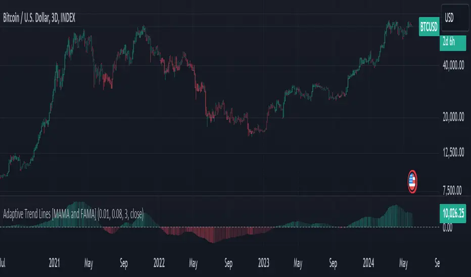
Advanced Fractal and Hurst IndicatorAdvanced Fractal and Hurst Indicator (AFHI)
Description:
The Advanced Fractal and Hurst Indicator (AFHI) is a custom technical analysis tool designed to identify market trends and potential reversals by leveraging the concepts of Fractal Dimension and the Hurst Exponent . These advanced mathematical concepts provide insights into the complexity and persistence of price movements, making this indicator a powerful addition to any trader's toolkit.
How It Works:
Fractal Dimension (FD) :
The Fractal Dimension measures the complexity of price movements. A higher Fractal Dimension indicates a more complex, choppy market, while a lower value suggests smoother trends.
The FD is calculated using the log difference of price movements over a specified length.
Hurst Exponent (HE) :
The Hurst Exponent indicates the tendency of a time series to either regress to the mean or cluster in a direction. Values below 0.5 indicate a tendency to revert to the mean (mean-reverting), while values above 0.5 suggest a trending market.
The HE is calculated using the rescaled range method, comparing the range of price movements to the standard deviation.
Composite Indicator :
The Composite Indicator combines the smoothed Fractal Dimension and Hurst Exponent to provide a single value indicating market conditions. This is done by normalizing the FD and HE values and combining them into one metric.
A positive Composite Indicator suggests an uptrend, while a negative value indicates a downtrend.
Smoothing :
Both FD and HE values are smoothed using a simple moving average to reduce noise and provide clearer signals.
Trend Confirmation :
A 50-period moving average (MA) is used to confirm the trend direction. The price being above the MA indicates an uptrend, while below the MA indicates a downtrend.
Background Shading :
The indicator pane is shaded green during uptrend conditions (positive Composite Indicator and price above MA) and red during downtrend conditions (negative Composite Indicator and price below MA).
How Traders Can Use It:
Identifying Trends :
Traders can use the AFHI to identify current market trends. The background shading in the indicator pane provides a visual cue for trend direction, with green indicating an uptrend and red indicating a downtrend.
Trend Confirmation :
The Composite Indicator line, plotted in purple, helps confirm the trend. Positive values suggest a strong uptrend, while negative values indicate a strong downtrend.
Entry and Exit Signals :
Traders can use the transitions of the Composite Indicator and the background shading to time their entry and exit points. For instance, a shift from red to green shading suggests a potential buy opportunity, while a shift from green to red suggests a potential sell opportunity.
Alerts :
The script includes alert conditions that can notify traders when the Composite Indicator signals a new trend direction. Alerts can be set up for both uptrends and downtrends, helping traders stay informed of key market changes.
Strategy Development :
By integrating AFHI into their trading strategies, traders can develop more robust systems that account for market complexity and persistence. The indicator can be used alongside other technical tools to enhance decision-making and improve trade accuracy.

Garman-Klass-Yang-Zhang Volatility EstimatorThe Garman-Klass-Yang-Zhang Volatility Estimator (GKYZVE) is yet another attempt to robustly measure volatility, integrating intra-candle and inter-candle dynamics. It is an extension of the Garman-Klass Volatility Estimator (GKVE) incorporating insights from the Yang-Zhang Volatility Estimator (YZVE) . Like the YZVE, the GKYZVE holistically considers open, high, low, and close prices. The formula for GKYZ is:
GKYZVE = 0.5 * σ_HL² + * σ_CC² + σ_OC²
Where:
σ_HL² is the variance based on the high and low prices (σ_HL² = (high - low)² / (4 * math.log(2))), weighted at 0.5.
σ_CC² is the close-to-close variance (σ_CC² = (close - close)²), weighted at (2 ln 2) -1 for the logarithmic distribution of returns and emphasizing the impact of day-to-day price changes.
σ_OC² is the variance of the opening price against the closing price (σ_OC² = 0.5 * (open - close)²), weighted at 1.
The GKYZVE differs from the YZVE by using fixed weighing factors derived from theoretical calculations, leaning heavier into the assumption that returns are log-distributed.
This script also offers a choice for normalization between 0 and 1, turning the estimator into an oscillator for comparing current volatility to recent levels. Horizontal lines at user-defined levels are also available for clearer visualization. Both options are off by default.
References:
Garman, M. B., & Klass, M. J. (1980). On the estimation of security price volatilities from historical data. The Journal of Business, 53(1), 67-78.
Yang, D., & Zhang, Q. (2000). Drift-independent volatility estimation based on high, low, open, and close prices. The Journal of Business, 73(3), 477-492.
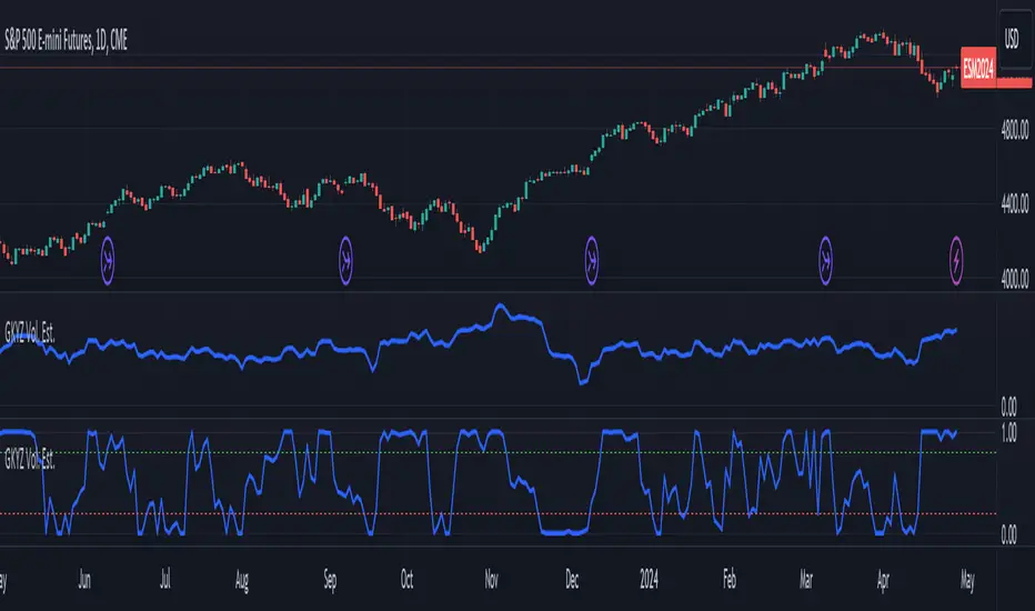
Unmitigated Liquidity Imbalances [AlgoAlpha]🎉 Introducing the Unmitigated Liquidity Imbalance Indicator by AlgoAlpha! 🎉
Dive into the depths of market analytics with our "Unmitigated Liquidity Imbalance" indicator. This tool harnesses unique algorithms to detect liquidity imbalances between bulls and bears, helping traders spot trends and potential entry and exit points with greater accuracy. 📈🚀
🔍 Key Features:
🌟 Advanced Analysis : Analyses candle direction and length to forecast market peaks and valleys.
🎨 Customizable Visuals : Tailor the chart with your choice of bullish green or bearish red to reflect different market conditions.
🔄 Real-Time Updates : Continuously updates to reflect live market changes.
🔔 Configurable Alerts : Set up alerts for key trading signals such as bullish and bearish reversals, as well as trend shifts.
📐 How to Use:
🛠 Add the Indicator : Add the indicator to your favourites and customize the settings to suite your needs.
📊 Market Analysis : Monitor the oscillator threshold; readings above 0.5 suggest bullish sentiment, while below 0.5 indicate bearish conditions. And reversal signals are displayed to show potential entry points.
🔔 Set Alerts : Enable notifications for reversal conditions or trend changes to seize trading opportunities without constant chart watching.
🧠 How It Works:
The core mechanism of the indicator is based on detecting changes in candlestick size and direction to identify bullish and bearish liquidity levels from the peak & valley indicator's logic. By comparing the length of a current candle to the previous one and checking the change in direction, it pinpoints moments where market sentiment could be shifting, indicating if the liquidity at that point is bullish or bearish. The script then looks at what percentage of the past few unmitigated levels are bullish or bearish based on a customizable lookback and determines the liquidity imbalance which can then be interpreted as trend.
Empower your trading with the Unmitigated Liquidity Imbalance indicator and navigate the markets with confidence and precision. 🌟💹
Happy trading, and may your charts be ever in your favour! 🥳✨
💎 Related Indicator

Turtle Trading Strategy@lihexieThe full implementation of the Turtle Trading Rules (as distinct from the various truncated versions circulating within the community) is now ready.
This trading strategy script distinguishes itself from all currently publicly available Turtle trading systems on Tradingview by comprehensively embodying the rules for entries, exits, position management, and profit and loss controls.
Market Selection:
Trade in highly liquid markets such as forex, commodity futures, and stock index futures.
Entry Strategies:
Model 1: Buy when the price breaks above the highest point of the last 20 trading days; Sell when the price drops below the lowest point of the last 20 trading days. When an entry opportunity arises, if the previous trade was profitable, skip the current breakout opportunity and refrain from entering.
Model 2: Buy when the price breaks above the highest point of the last 55 trading days; Sell when the price drops below the lowest point of the last 55 trading days.
Position Sizing:
Determine the size of each position based on the price volatility (ATR) to ensure that the risk of each trade does not exceed 2% of the account balance.
Exit Strategies:
1. Use a fixed stop-loss point to limit losses: Close long positions when the price falls below the lowest point of the last 10 trading days.
2. Trailing stop-loss: Once a position is profitable, adjust the stop-loss point to protect profits.
Pyramiding Rules:
Unit Doubling: Increase position size by one unit every time the price moves forward by n (default is 0.5) units of ATR, up to a maximum of 4 units, while also raising the stop-loss point to below the ATR value at the level of additional entries.
海龟交易法则的完整实现(区别于当前社区各种有阉割海龟交易系统代码)
本策略脚本区别于Tradingview目前公开的所有的海龟交易系统,完整的实现了海龟交易法则中入场、出场、仓位管理,止盈止损的规则。
市场选择:
选择流动性高的市场进行交易,如外汇、商品期货和股指期货等。
入市策略:
模式1:当价格突破过去20个交易日的高点时,买入;当价格跌破过去20个交易日的低点时,卖出。当出现入场机会时,如果上一笔交易是盈利的,那么跳过当前突破的机会,不进行入场。
模式2:当价格突破过去55个交易日的高点时,买入;当价格跌破过去55个交易日的低点时,卖出。
头寸规模:
根据价格波动性(ATR)来确定每个头寸的大小, 使每笔交易的风险不超过账户余额的2%。
退出策略:
1. 使用一个固定的止损点来限制损失:当多头头寸的价格跌破过去10个交易日的低点时,平仓止损。
2. 跟踪止损:一旦头寸盈利,移动止损点以保护利润。
加仓规则:
单位加倍:每当价格向前n(默认是0.5)个单位的ATR移动时,就增加一个单位的头寸大小(默认最大头寸数量是4个),同时将止损点提升至加仓点位的ATR值以下。

ottlibLibrary "ottlib"
█ OVERVIEW
This library contains functions for the calculation of the OTT (Optimized Trend Tracker) and its variants, originally created by Anıl Özekşi (Anil_Ozeksi). Special thanks to him for the concept and to Kıvanç Özbilgiç (KivancOzbilgic) and dg_factor (dg_factor) for adapting them to Pine Script.
█ WHAT IS "OTT"
The OTT (Optimized Trend Tracker) is a highly customizable and very effective trend-following indicator that relies on moving averages and a trailing stop at its core. Moving averages help reduce noise by smoothing out sudden price movements in the markets, while trailing stops assist in detecting trend reversals with precision. Initially developed as a noise-free trailing stop, the current variants of OTT range from rapid trend reversal detection to long-term trend confirmation, thanks to its extensive customizability.
It's well-known variants are:
OTT (Optimized Trend Tracker).
TOTT (Twin OTT).
OTT Channels.
RISOTTO (RSI OTT).
SOTT (Stochastic OTT).
HOTT & LOTT (Highest & Lowest OTT)
ROTT (Relative OTT)
FT (Original name is Fırsatçı Trend in Turkish which translates to Opportunist Trend)
█ LIBRARY FEATURES
This library has been prepared in accordance with the style, coding, and annotation standards of Pine Script version 5. As a result, explanations and examples will appear when users hover over functions or enter function parameters in the editor.
█ USAGE
Usage of this library is very simple. Just import it to your script with the code below and use its functions.
import ismailcarlik/ottlib/1 as ottlib
█ FUNCTIONS
• f_vidya(source, length, cmoLength)
Short Definition: Chande's Variable Index Dynamic Average (VIDYA).
Details: This function computes Chande's Variable Index Dynamic Average (VIDYA), which serves as the original moving average for OTT. The 'length' parameter determines the number of bars used to calculate the average of the given source. Lower values result in less smoothing of prices, while higher values lead to greater smoothing. While primarily used internally in this library, it has been made available for users who wish to utilize it as a moving average or use in custom OTT implementations.
Parameters:
source (float) : (series float) Series of values to process.
length (simple int) : (simple int) Number of bars to lookback.
cmoLength (simple int) : (simple int) Number of bars to lookback for calculating CMO. Default value is `9`.
Returns: (float) Calculated average of `source` for `length` bars back.
Example:
vidyaValue = ottlib.f_vidya(source = close, length = 20)
plot(vidyaValue, color = color.blue)
• f_mostTrail(source, multiplier)
Short Definition: Calculates trailing stop value.
Details: This function calculates the trailing stop value for a given source and the percentage. The 'multiplier' parameter defines the percentage of the trailing stop. Lower values are beneficial for catching short-term reversals, while higher values aid in identifying long-term trends. Although only used once internally in this library, it has been made available for users who wish to utilize it as a traditional trailing stop or use in custom OTT implementations.
Parameters:
source (float) : (series int/float) Series of values to process.
multiplier (simple float) : (simple float) Percent of trailing stop.
Returns: (float) Calculated value of trailing stop.
Example:
emaValue = ta.ema(source = close, length = 14)
mostValue = ottlib.f_mostTrail(source = emaValue, multiplier = 2.0)
plot(mostValue, color = emaValue >= mostValue ? color.green : color.red)
• f_ottTrail(source, multiplier)
Short Definition: Calculates OTT-specific trailing stop value.
Details: This function calculates the trailing stop value for a given source in the manner used in OTT. Unlike a traditional trailing stop, this function modifies the traditional trailing stop value from two bars prior by adjusting it further with half the specified percentage. The 'multiplier' parameter defines the percentage of the trailing stop. Lower values are beneficial for catching short-term reversals, while higher values aid in identifying long-term trends. Although primarily used internally in this library, it has been made available for users who wish to utilize it as a trailing stop or use in custom OTT implementations.
Parameters:
source (float) : (series int/float) Series of values to process.
multiplier (simple float) : (simple float) Percent of trailing stop.
Returns: (float) Calculated value of OTT-specific trailing stop.
Example:
vidyaValue = ottlib.f_vidya(source = close, length = 20)
ottValue = ottlib.f_ottTrail(source = vidyaValue, multiplier = 1.5)
plot(ottValue, color = vidyaValue >= ottValue ? color.green : color.red)
• ott(source, length, multiplier)
Short Definition: Calculates OTT (Optimized Trend Tracker).
Details: The OTT consists of two lines. The first, known as the "Support Line", is the VIDYA of the given source. The second, called the "OTT Line", is the trailing stop based on the Support Line. The market is considered to be in an uptrend when the Support Line is above the OTT Line, and in a downtrend when it is below.
Parameters:
source (float) : (series float) Series of values to process. Default value is `close`.
length (simple int) : (simple int) Number of bars to lookback. Default value is `2`.
multiplier (simple float) : (simple float) Percent of trailing stop. Default value is `1.4`.
Returns: ( [ float, float ]) Tuple of `supportLine` and `ottLine`.
Example:
= ottlib.ott(source = close, length = 2, multiplier = 1.4)
longCondition = ta.crossover(supportLine, ottLine)
shortCondition = ta.crossunder(supportLine, ottLine)
• tott(source, length, multiplier, bandsMultiplier)
Short Definition: Calculates TOTT (Twin OTT).
Details: TOTT consists of three lines: the "Support Line," which is the VIDYA of the given source; the "Upper Line," a trailing stop of the Support Line adjusted with an added multiplier; and the "Lower Line," another trailing stop of the Support Line, adjusted with a reduced multiplier. The market is considered in an uptrend if the Support Line is above the Upper Line and in a downtrend if it is below the Lower Line.
Parameters:
source (float) : (series float) Series of values to process. Default value is `close`.
length (simple int) : (simple int) Number of bars to lookback. Default value is `40`.
multiplier (simple float) : (simple float) Percent of trailing stop. Default value is `0.6`.
bandsMultiplier (simple float) : Multiplier for bands. Default value is `0.0006`.
Returns: ( [ float, float, float ]) Tuple of `supportLine`, `upperLine` and `lowerLine`.
Example:
= ottlib.tott(source = close, length = 40, multiplier = 0.6, bandsMultiplier = 0.0006)
longCondition = ta.crossover(supportLine, upperLine)
shortCondition = ta.crossunder(supportLine, lowerLine)
• ott_channel(source, length, multiplier, ulMultiplier, llMultiplier)
Short Definition: Calculates OTT Channels.
Details: OTT Channels comprise nine lines. The central line, known as the "Mid Line," is the OTT of the given source's VIDYA. The remaining lines are positioned above and below the Mid Line, shifted by specified multipliers.
Parameters:
source (float) : (series float) Series of values to process. Default value is `close`
length (simple int) : (simple int) Number of bars to lookback. Default value is `2`
multiplier (simple float) : (simple float) Percent of trailing stop. Default value is `1.4`
ulMultiplier (simple float) : (simple float) Multiplier for upper line. Default value is `0.01`
llMultiplier (simple float) : (simple float) Multiplier for lower line. Default value is `0.01`
Returns: ( [ float, float, float, float, float, float, float, float, float ]) Tuple of `ul4`, `ul3`, `ul2`, `ul1`, `midLine`, `ll1`, `ll2`, `ll3`, `ll4`.
Example:
= ottlib.ott_channel(source = close, length = 2, multiplier = 1.4, ulMultiplier = 0.01, llMultiplier = 0.01)
• risotto(source, length, rsiLength, multiplier)
Short Definition: Calculates RISOTTO (RSI OTT).
Details: RISOTTO comprised of two lines: the "Support Line," which is the VIDYA of the given source's RSI value, calculated based on the length parameter, and the "RISOTTO Line," a trailing stop of the Support Line. The market is considered in an uptrend when the Support Line is above the RISOTTO Line, and in a downtrend if it is below.
Parameters:
source (float) : (series float) Series of values to process. Default value is `close`.
length (simple int) : (simple int) Number of bars to lookback. Default value is `50`.
rsiLength (simple int) : (simple int) Number of bars used for RSI calculation. Default value is `100`.
multiplier (simple float) : (simple float) Percent of trailing stop. Default value is `0.2`.
Returns: ( [ float, float ]) Tuple of `supportLine` and `risottoLine`.
Example:
= ottlib.risotto(source = close, length = 50, rsiLength = 100, multiplier = 0.2)
longCondition = ta.crossover(supportLine, risottoLine)
shortCondition = ta.crossunder(supportLine, risottoLine)
• sott(source, kLength, dLength, multiplier)
Short Definition: Calculates SOTT (Stochastic OTT).
Details: SOTT is comprised of two lines: the "Support Line," which is the VIDYA of the given source's Stochastic value, based on the %K and %D lengths, and the "SOTT Line," serving as the trailing stop of the Support Line. The market is considered in an uptrend when the Support Line is above the SOTT Line, and in a downtrend when it is below.
Parameters:
source (float) : (series float) Series of values to process. Default value is `close`.
kLength (simple int) : (simple int) Stochastic %K length. Default value is `500`.
dLength (simple int) : (simple int) Stochastic %D length. Default value is `200`.
multiplier (simple float) : (simple float) Percent of trailing stop. Default value is `0.5`.
Returns: ( [ float, float ]) Tuple of `supportLine` and `sottLine`.
Example:
= ottlib.sott(source = close, kLength = 500, dLength = 200, multiplier = 0.5)
longCondition = ta.crossover(supportLine, sottLine)
shortCondition = ta.crossunder(supportLine, sottLine)
• hottlott(length, multiplier)
Short Definition: Calculates HOTT & LOTT (Highest & Lowest OTT).
Details: HOTT & LOTT are composed of two lines: the "HOTT Line", which is the OTT of the highest price's VIDYA, and the "LOTT Line", the OTT of the lowest price's VIDYA. A high price surpassing the HOTT Line can be considered a long signal, while a low price dropping below the LOTT Line may indicate a short signal.
Parameters:
length (simple int) : (simple int) Number of bars to lookback. Default value is `20`.
multiplier (simple float) : (simple float) Percent of trailing stop. Default value is `0.6`.
Returns: ( [ float, float ]) Tuple of `hottLine` and `lottLine`.
Example:
= ottlib.hottlott(length = 20, multiplier = 0.6)
longCondition = ta.crossover(high, hottLine)
shortCondition = ta.crossunder(low, lottLine)
• rott(source, length, multiplier)
Short Definition: Calculates ROTT (Relative OTT).
Details: ROTT comprises two lines: the "Support Line", which is the VIDYA of the given source, and the "ROTT Line", the OTT of the Support Line's VIDYA. The market is considered in an uptrend if the Support Line is above the ROTT Line, and in a downtrend if it is below. ROTT is similar to OTT, but the key difference is that the ROTT Line is derived from the VIDYA of two bars of Support Line, not directly from it.
Parameters:
source (float) : (series float) Series of values to process. Default value is `close`.
length (simple int) : (simple int) Number of bars to lookback. Default value is `200`.
multiplier (simple float) : (simple float) Percent of trailing stop. Default value is `0.1`.
Returns: ( [ float, float ]) Tuple of `supportLine` and `rottLine`.
Example:
= ottlib.rott(source = close, length = 200, multiplier = 0.1)
isUpTrend = supportLine > rottLine
isDownTrend = supportLine < rottLine
• ft(source, length, majorMultiplier, minorMultiplier)
Short Definition: Calculates Fırsatçı Trend (Opportunist Trend).
Details: FT is comprised of two lines: the "Support Line", which is the VIDYA of the given source, and the "FT Line", a trailing stop of the Support Line calculated using both minor and major trend values. The market is considered in an uptrend when the Support Line is above the FT Line, and in a downtrend when it is below.
Parameters:
source (float) : (series float) Series of values to process. Default value is `close`.
length (simple int) : (simple int) Number of bars to lookback. Default value is `30`.
majorMultiplier (simple float) : (simple float) Percent of major trend. Default value is `3.6`.
minorMultiplier (simple float) : (simple float) Percent of minor trend. Default value is `1.8`.
Returns: ( [ float, float ]) Tuple of `supportLine` and `ftLine`.
Example:
= ottlib.ft(source = close, length = 30, majorMultiplier = 3.6, minorMultiplier = 1.8)
longCondition = ta.crossover(supportLine, ftLine)
shortCondition = ta.crossunder(supportLine, ftLine)
█ CUSTOM OTT CREATION
Users can create custom OTT implementations using f_ottTrail function in this library. The example code which uses EMA of 7 period as moving average and calculates OTT based of it is below.
Source Code:
//@version=5
indicator("Custom OTT", shorttitle = "COTT", overlay = true)
import ismailcarlik/ottlib/1 as ottlib
src = input.source(close, title = "Source")
length = input.int(7, title = "Length", minval = 1)
multiplier = input.float(2.0, title = "Multiplier", minval = 0.1)
support = ta.ema(source = src, length = length)
ott = ottlib.f_ottTrail(source = support, multiplier = multiplier)
pSupport = plot(support, title = "Moving Average Line (Support)", color = color.blue)
pOtt = plot(ott, title = "Custom OTT Line", color = color.orange)
fillColor = support >= ott ? color.new(color.green, 60) : color.new(color.red, 60)
fill(pSupport, pOtt, color = fillColor, title = "Direction")
Result:
█ DISCLAIMER
Trading is risky and most of the day traders lose money eventually. This library and its functions are only for educational purposes and should not be construed as financial advice. Past performances does not guarantee future results.
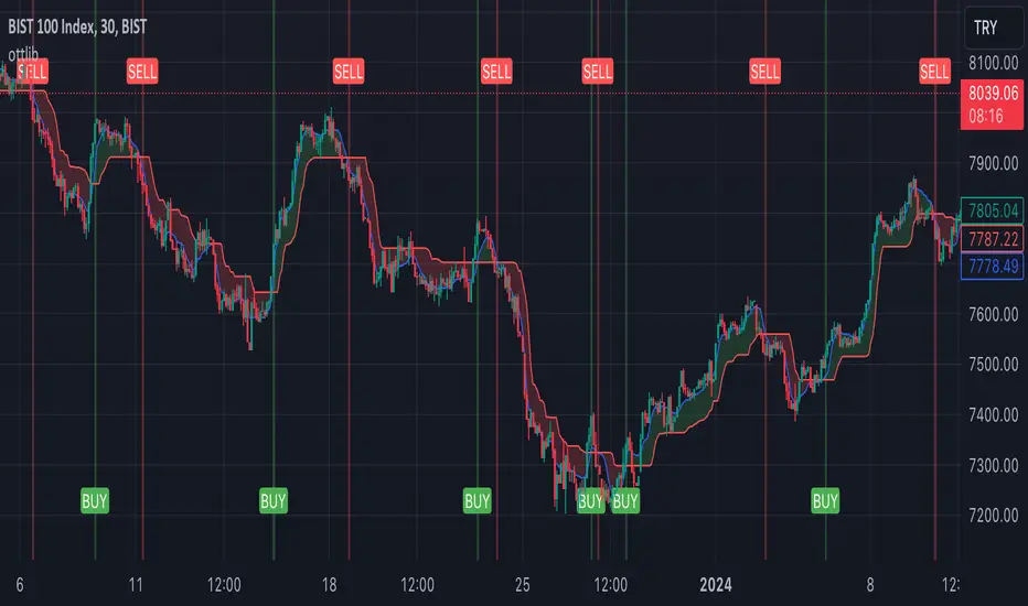
FX DispersionThis script calculates the dispersion of a basket of 5 FX pairs and then calculates the z-score the z-score is then made into a composite using the 30 and 60 ema of the z-score to smooth any noise. It must be used on one of the FX pairs in the basket and on the 1-minute timeframe as it has been hardcoded for 1 min use below.
Interpretation - Dispersion is a component of volatility - the dispersion of the underlying basket increases above 0.5 and decreases below 0.5.
Although increased dispersion is beneficial to momentum and trend-following strategies on the monthly and weekly timeframes. Observe this on the 1-minute timeframe and how dispersion crossing above/ below 0.5 it can signal reversion or momentum for the next period.
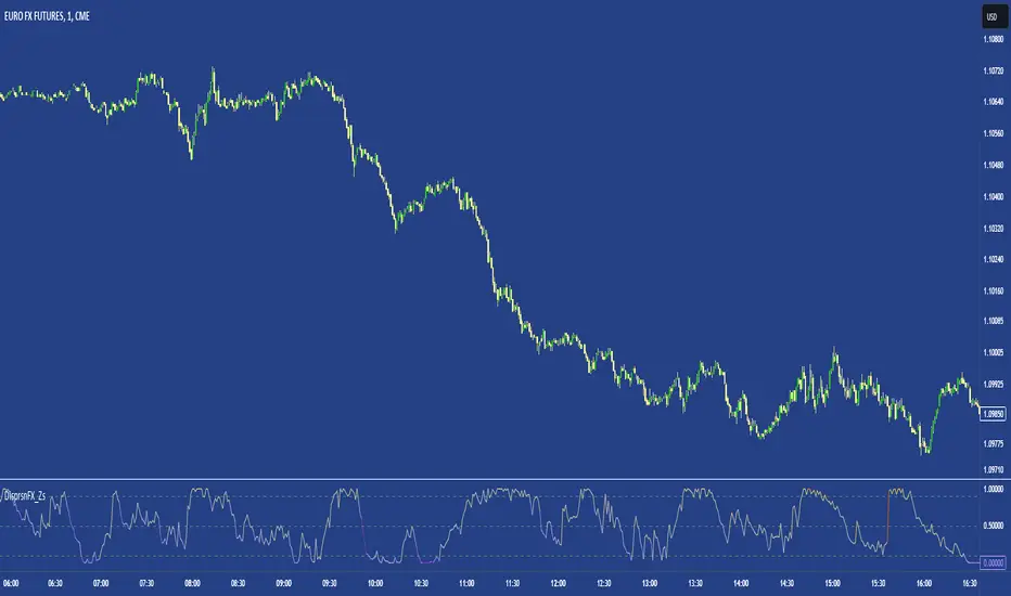
[PUZ]Relativ Strength Index [MTB]Here I provide you with my new RSI indicator.
This RSI has some advantages over the normal Tadingview RSI.
The RSI is usually calculated exclusively on a Candel Close basis. My RSI is calculated on a Candel Close, Open, High, Low basis, which makes it look a little smoother. Furthermore, there are not only 3 support and resistance lines but a total of 7 where the rsi can bounce. These lines can all be set variably under the Style settings.
In addition, the RSI also shows divergences and hidden divergences via red and blue lines.
There is also the option to make trend settings
Option one involves determining the trend based on various selectable moving averages. You can also select the time frame for trend determination.
The trend is shown by coloring the background in the RSI green and red. Of course you can also switch the background on and off.
The second trend option is to determine a Fibbonacci line which is displayed red or green on LVL 100 depending on the trend direction.
In this trend calculation you can also select the time frame yourself and you can use the sensitivity to determine how many previous candels are taken into account to determine the trend.
If a candel close occurs above the 0.5 and 0.236 Fibb LVL, the trend turns green.
If a candel close occurs below the 0.5 and 0.786 Fibb LVL, the trend turns red.
A final additional feature is an output module where the RSI data is scaled between 0 and 1 in order to further process this data in future scripts.
A huge thank you goes out to djmad for providing his math library and another thank you to jdehorty for providing his MLExtension library
