72s Strat: Backtesting Adaptive HMA+ pt.1This is a follow up to my previous publication of Adaptive HMA+ few months ago, as a mean to provide some kind of initial backtesting tools. Which can be use to explore many possible strategies, optimise its settings to better conform user's pair/tf, and hopefully able to help tweaking your general strategy.
If you haven't read the study or use the indicator, kindly go here first to get the overall idea.
The first strategy introduce in this backtest is one most basic already described in the study; buy/sell is when movement is there and everything is on the right side; When RSI has turned to other side, we can use it as exit point (if in profit of course, else just let it hit our TP/SL, why would we exit before profit). Also, base on RSI when we make entry, we can further differentiate type of signals. --Please check all comments in code directly where the signals , entries , and exits section are.
Second additional strategy to check; is when we also use second faster Adaptive HMA+ for exit. So this is like a double orders on a signal but with different exit-rule (/more on this on snapshots below). Alternatively, you can also work the code so to only use this type of exit.
There's also an additional feature which you can enable its visuals, the Distance Zone , is to help measuring price distance to our xHMA+. It's just a simple atr based envelope really, I already put the sample code in study's comment section, but better gonna update it there directly for non-coder too, after this.
In this sample I use Lot for order quantity size just because that's what I use on my broker. Also what few friends use while we forward-testing it since the study is published, so we also checked/compared each profit/loss report by real number. To use default or other unit of measurement, change the entry code accordingly.
If you change your order size, you should also change the commission in Properties Tab. My broker commission is 5 USD per order/lot, so in there with example order size 0.1 lot I put commission 0.5$ per order (I'll put 2.5$ for 0.5 lot, 10$ for 2 lot, and so on). Crypto usually has higher charge. --It is important that you should fill it base on your broker.
SETTINGS
I'm trying to keep it short. Please explore it further again. (Beginner should also first get acquaintance with terms use here.)
ORDERS:
Base Minimum Profit Before Exit:
The number is multiplier of ongoing ATR. Means that when basic exit condition is met, algo will check whether you're already in minimum profit or not, if not, let it still run to TP or SL, or until it meets subsequent exit condition, then it will check again.
Default Target Profit:
Multiplier of ATR at signal. If reached before any eligible exit condition is met, exit TP.
Base StopLoss Point:
You can change directly in code to use other like ATR Trailing SL, fix percent SL, or whatever. In the sample, 4 options provided.
Maximum StopLoss:
This is like a safety-net, that if at some point your chosen SL point from input above happens to be exceeding this maximum input that you can tolerate, then this max point is the one will be use as SL.
Activate 2nd order...:
The additional doubling of certain buy/sell with different exits as described above. If enable, you should also set pyramiding to at least: 2. If not, it does nothing.
ADAPTIVE HMA+ PERIOD
Many users already have their own settings for these. So in here I only sample the default as first presented in the study. Make it to your adaptive.
MARKET MOVEMENT
(1) Now you can check in realtime how much slope degree is best to define your specific pair/tf is out of congestion (yellow) area. And (2) also able to check directly what ATR lengths are more suitable defining your pair's volatility.
DISTANCE ZONE
Distance Multiplier. Each pair/tf has its own best distance zone (in xHMA+ perspective). The zone also determine whether a signal should appear or not. (Or what type of signal, if you wanna go more detail in constructing your strategy)
USAGE
(Provided you already have your own comfortable settings for minimum-maximum period of Adaptive HMA+. Best if you already have backtested it manually too and/or apply as an add-on to your working strategy)
1. In our experiences, first most important to define is both elements in the Market Movement Settings . These also tend to be persistent for whole season since it's kinda describing that pair/tf overall behaviour. Don't worry if you still get a low Profit Factor here, but by tweaking you should start to see positive changes in one of Max Drawdown and Net Profit, or Percent Profitable.
2. Afterwards, find your pair/tf Distance Zone . When optimising this, what we seek is just a "not to bad" equity curves to start forming. At least Max Drawdown should lessen more. Doesn't have to be great already, but should be better, no red in Net Profit.
3. Then go manage the "Trailing Minimum Profit", TP, SL, and max SL.
4. Repeat 1,2,3. 👻
5. Manage order size, commission, and/or enable double-order (need pyramiding) if you like. Check if your equity can handle max drawdown before margin call.
6. After getting an acceptable backtest result, go to List of Trades tab and find the biggest loss or when many sequencing loss in a row happened. Click on it to go to exact point on chart, observe why the signal failed and get at least general idea how it can be prevented . The rest is yours, you should know your pair/tf more than other.
You can also re-explore your minimum-maximum period for both Major and minor xHMA+.
Keep in mind that all numbers in Setting are conceptually in a form of range . You don't want to get superb equity curves but actually a "fragile" , means one can easily turn it to disaster just by changing only a fraction in one/two of the setting.
---
If you just wanna test the strength of the indicator alone, you can disable "Use StopLoss" temporarily while optimising settings.
Using no SL might be tempting in overall result data in some cases, but NOTE: It is not recommended to not using SL, don't forget that we deliberately enter when it's in high volatility. If want to add flexibility or trading for long-term, just maximise your SL. ie.: chose SL Point>ATR only and set it maximum. (Check your max drawdown after this).
I think this is quite important specially for beginners, so here's an example; Hypothetically in below scenario, because of some settings, the buy order after the loss sell signal didn't appear. Let's say if our initial capital only 1000$ using leverage and order size 0,5 lot (risky position sizing already), moreover if this happens at the beginning of your trading season, that's half of account gone already in one trade . Your max SL should've made you exit after that pumping bar.
The Trailing Minimum Profit is actually look like this. Search in the code if you want to plot it. I just don't like too many lines on chart.
To maximise profit we can try enabling double-order. The only added rule coded is: RSI should rising when buy and falling when sell. 2nd signal will appears above or below default buy/sell signal. (Of course it's also prone to double-loss, re-check your max drawdown after. Profit factor play its part in here for a long run). Snapshot in comparison:
Two default sell signals on left closed at RSI exit, the additional sell signal closed later on when price crossover minor xHMA+. On buy side, price haven't met our minimum profit when first crossunder minor xHMA+. If later on we hit SL on this "+buy" signal, at least we already profited from default buy signal. You can also consider/treat this as multiple TP points.
For longer-term trading, what you need to maximise is the Minimum Profit , so it won't exit whenever an exit condition happened, it can happen several times before reaching minimum profit. Hopefully this snapshot can explain:
Notice in comparison default sell and buy signal now close in average after 3 days. What's best is when we also have confirmation from higher TF. It's like targeting higher TF by entering from smaller TF.
As also mention in the study, we can still experiment via original HMA by putting same value for minimum-maximum period setting. This is experimental EU 1H with Major xHMA+: 144-144, Flat market 13, Distance multiplier 3.6, with 2nd order activated.
Kiwi was a bit surprising for me. It's flat market is effectively below 6, with quite far distance zone of 3.5. Probably because I'm using big numbers in adaptive period.
---
The result you see in strategy tester report below for EURUSD 15m is using just default settings you see in code, as follow:
0,1 lot for each order (which is the smallest allowed by my broker).
No pyramiding. Commission: 0.5 usd per order. Slippage: 3
Opening position is only using basic strategy #1 (RSI exit). Additional exit not activated.
Minimum Profit: 1. TP: 3.
SL use: Half-distance zone. Max SL: 4.5.
Major xHMA+: 172-233. minor xHMA+: 89-121
Distance Zone Multiplier: 2.7
RSI: Standard 14.
(From our forward-testing, the difference we get from net profit is because of the spread, our entry isn't exactly at the close/open price. Not so much though, but not the same. If somebody can direct me to any example where we can code our entry via current bid/ask price, that would be awesome!)
It's already a long post (sorry), think I'm gonna pause here. Check out the code :)
---
DISCLAIMER: Past performance is no guarantee of future results , and so on.. you know the drill ;)
Please read whole description first before using, don't take 1-2 paragraph and claim it's the whole logic, you are responsible of your own actions and understanding.
Komut dosyalarını "通达信+选股公式+换手率+0.5+源码" için ara

Hurst ExponentMy first try to implement Full Hurst Exponent.
The Hurst exponent is used as a measure of long-term memory of time series. It relates to the autocorrelations of the time series and the rate at which these decrease as the lag between pairs of values increases
The Hurst exponent is referred to as the "index of dependence" or "index of long-range dependence". It quantifies the relative tendency of a time series either to regress strongly to the mean or to cluster in a direction.
In short, depending on the value you can spot the trending / reversing market.
Values 0.5 to 1 - market trending
Values 0 to 0.5 - market tend to mean revert
Hurst Exponent is computed using Rescaled range (R/S) analysis.
I split the lookback period (N) in the number of shorter samples (for ex. N/2, N/4, N/8, etc.). Then I calculate rescaled range for each sample size.
The Hurst exponent is estimated by fitting the power law. Basically finding the slope of log(samples_size) to log(RS).
You can choose lookback and sample sizes yourself. Max 8 possible at the moment, if you want to use less use 0 in inputs.
It's pretty computational intensive, so I added an input so you can limit from what date you want it to be calculated. If you hit the time limit in PineScript - limit the history you're using for calculations.
####################
Disclaimer
Please remember that past performance may not be indicative of future results.
Due to various factors, including changing market conditions, the strategy may no longer perform as good as in historical backtesting.
This post and the script don’t provide any financial advice.

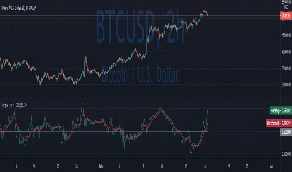
Simple Hurst Exponent [QuantNomad]This is a simplified version of the Hurst Exponent indicator.
In the meantime, I'm working on the full version. It's computationally intensive, so it's a challenge to squeeze it to PineScript limits. It will require some time to optimize it, so I decided to publish a simplified version for now.
The Hurst exponent is used as a measure of long-term memory of time series. It relates to the autocorrelations of the time series, and the rate at which these decrease as the lag between pairs of values increases
The Hurst exponent is referred to as the "index of dependence" or "index of long-range dependence". It quantifies the relative tendency of a time series either to regress strongly to the mean or to cluster in a direction.
In short depend on value you can spot trending / reversing market.
Values 0.5 to 1 - market trending
Values 0 to 0.5 - market tend to mean revert
####################
Disclaimer
Please remember that past performance may not be indicative of future results.
Due to various factors, including changing market conditions, the strategy may no longer perform as good as in historical backtesting.
This post and the script don’t provide any financial advice.
Pin Bar CandlesPinbar Identification.
One must apply Fibonacchi extension 0,0.5,1,2, 3, 4.
0 being SL
1 Being Entry
0.5 Being 2nd Entry.
4 Being target.
Use this to enter trade near crucial levels only.

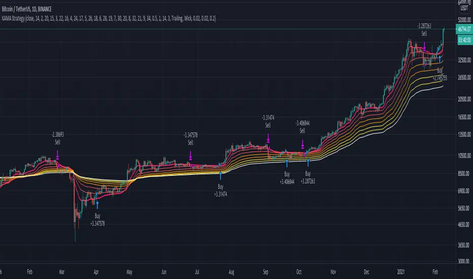
KAMA Strategy - Kaufman's Adaptive Moving AverageThis strategy combines Kaufman's Adaptive Moving Average for entry with optional KAMA, PSAR, and Trailing ATR stops for exits.
Kaufman's Adaptive Moving Average is, in my opinion, a gem among the plethora of indicators. It is underrated considering it offers a solution that intuitively makes a lot of sense. When I first read about it, it was a real 'aha!' moment. Look at the top, pink line. Notice how during trending times it follows the trend quickly and closely, but during choppy, non-trending periods, the KAMA stays absolutely flat? Interesting! To trade with it, we simply follow the direction the KAMA is pointing. Is it up? Go long. Is it down? Go short. Is it flat? Hold on.
How does it manage to quickly follow real trends like a fast EMA but ignore choppy conditions that would whipsaw a fast EMA back and forth? It analyses whether recent price moves are significant relative to recent noise and then adapts the length of the EMA window accordingly. If price movement is big compared to the recent noise, the EMA window gets smaller. If price movement is relatively small or average compared to the recent noise, the EMA window gets bigger. In practice it means:
The KAMA would be flat if a 20 point upwards move occurred during a period that has had, on average, regular 20 point moves BUT
the KAMA would point up if a 20 point move occurred during a period that has, on average, had moves of only around 5 points.
In other words, it's a slow EMA during choppy flat / quiet flat periods, and a fast EMA as soon as significant volatility occurs. Perfect!
-----
The Strategy
The strategy is more than just a KAMA indicator. It contains:
KAMA exit (optional)
ATR trailing stop loss exit (optional)
PSAR stop loss exit (optional)
KAMA filter for entry and exits
All features are adjustable in the strategy settings
The Technical Details:
Check out the strategy's 'Inputs' panel. The buy and sell signals are based on the 'KAMA 1' there.
KAMA 1: Length -- 14 is the default. This is the length of the window the KAMA looks back over. In this instance, it c
KAMA 1: Fast KAMA Length -- 2 is the default. This is the tightest the EMA length is allowed to get. It will tend towards this length when volatility is high.
KAMA 1: Slow KAMA Length -- 20 is the default. This is the biggest the EMA length is allowed to get. It will tend towards this length when volatility is low.
KAMA Filter
The strategy buys when the KAMA begins to point up and sells when the KAMA points down. Generally, the KAMA is very good at filtering out the noise itself - it will go flat during noisy/choppy periods. But to add another layer of safety, its author, Perry Kaufman, proposed a KAMA filter. It works by taking the standard deviation of returns over the length of the the 'KAMA 1: Length' I mentioned above and multiplying it by an 'Entry Filter' (1 by default) and 'Exit Filter' (0.5 by default). The entry condition to go long is that the KAMA is pointing up and and it moved up more than 1 x St. Dev. of Returns. The exit condition is when the KAMA is pointing down and it moved down by more than 0.5 x St. Dev. of Returns.
Thanks
Thanks to ChuckBanger, cheatcountry, millerrh, and racer8 for parts of the code. I was able to build upon their good work.
-----
I hope this strategy is helpful to you.
Do you have any thoughts, ideas, or questions? Let me know in the comments or send me a message! I'd be glad to help you out.
If you need an indicator or strategy to be built or customised for you, let me know! I'll be glad to help and it'll probably be cheaper than you think!
[blackcat] L2 Ehlers DFT Spectral EstimateLevel: 2
Background
John F. Ehlers introduced DFT Spectral Estimate in his "Cycle Analytics for Traders" chapter 9 on 2013.
Function
The DFT is accomplished by correlating the data with the cosine and sine of each period of interest over the selected window period. The sum of the squares of each of these correlated values represents the relative power at each period. The only user input is whether to select Spectral Dilation compensation. The default selection is NOT to use the compensation.
The spectrum values vary between 0 and 1 after being normalized. These values are converted to colors. When the spectrum is greater than 0.5 the colors combine red and yellow, with yellow being the result when spectrum = 1 and red being the result when the spectrum = 0.5. When the spectrum is less than 0.5, the red saturation is decreased, with the result that the color is black when spectrum = 0.
Key Signal
DominantCycle --> Dominant Cycle signal
Pros and Cons
100% John F. Ehlers definition translation of original work, even variable names are the same. This help readers who would like to use pine to read his book. If you had read his works, then you will be quite familiar with my code style.
Remarks
The 51th script for Blackcat1402 John F. Ehlers Week publication.
Readme
In real life, I am a prolific inventor. I have successfully applied for more than 60 international and regional patents in the past 12 years. But in the past two years or so, I have tried to transfer my creativity to the development of trading strategies. Tradingview is the ideal platform for me. I am selecting and contributing some of the hundreds of scripts to publish in Tradingview community. Welcome everyone to interact with me to discuss these interesting pine scripts.
The scripts posted are categorized into 5 levels according to my efforts or manhours put into these works.
Level 1 : interesting script snippets or distinctive improvement from classic indicators or strategy. Level 1 scripts can usually appear in more complex indicators as a function module or element.
Level 2 : composite indicator/strategy. By selecting or combining several independent or dependent functions or sub indicators in proper way, the composite script exhibits a resonance phenomenon which can filter out noise or fake trading signal to enhance trading confidence level.
Level 3 : comprehensive indicator/strategy. They are simple trading systems based on my strategies. They are commonly containing several or all of entry signal, close signal, stop loss, take profit, re-entry, risk management, and position sizing techniques. Even some interesting fundamental and mass psychological aspects are incorporated.
Level 4 : script snippets or functions that do not disclose source code. Interesting element that can reveal market laws and work as raw material for indicators and strategies. If you find Level 1~2 scripts are helpful, Level 4 is a private version that took me far more efforts to develop.
Level 5 : indicator/strategy that do not disclose source code. private version of Level 3 script with my accumulated script processing skills or a large number of custom functions. I had a private function library built in past two years. Level 5 scripts use many of them to achieve private trading strategy.

[blackcat] L2 Ehlers Autocorrelation PeriodogramLevel: 2
Background
John F. Ehlers introduced Autocorrelation Periodogram in his "Cycle Analytics for Traders" chapter 8 on 2013.
Function
Construction of the autocorrelation periodogram starts with the autocorrelation function using the minimum three bars of averaging. The cyclic information is extracted using a discrete Fourier transform (DFT) of the autocorrelation results. This approach has at least four distinct advantages over other spectral estimation techniques. These are:
1. Rapid response. The spectral estimates start to form within a half-cycle period of their initiation.
2. Relative cyclic power as a function of time is estimated. The autocorrelation at all cycle periods can be low if there are no cycles present, for example, during a trend. Previous works treated the maximum cycle amplitude at each time bar equally.
3. The autocorrelation is constrained to be between minus one and plus one regardless of the period of the measured cycle period. This obviates the need to compensate for Spectral Dilation of the cycle amplitude as a function of the cycle period.
4. The resolution of the cyclic measurement is inherently high and is independent of any windowing function of the price data.
The dominant cycle is extracted from the spectral estimate in the next block of code using a center-of-gravity (CG) algorithm. The CG algorithm measures the average center of two-dimensional objects. The algorithm computes the average period at which the powers are centered. That is the dominant cycle. The dominant cycle is a value that varies with time. The spectrum values vary between 0 and 1 after being normalized. These values are converted to colors. When the spectrum is greater than 0.5, the colors combine red and yellow, with yellow being the result when spectrum = 1 and red being the result when the spectrum = 0.5. When the spectrum is less than 0.5, the red saturation is decreased, with the result the color is black when spectrum = 0.
Key Signal
DominantCycle --> Dominant Cycle
Period --> Autocorrelation Periodogram Array
Pros and Cons
100% John F. Ehlers definition translation of original work, even variable names are the same. This help readers who would like to use pine to read his book. If you had read his works, then you will be quite familiar with my code style.
Remarks
The 49th script for Blackcat1402 John F. Ehlers Week publication.
Courtesy of @RicardoSantos for RGB functions.
Readme
In real life, I am a prolific inventor. I have successfully applied for more than 60 international and regional patents in the past 12 years. But in the past two years or so, I have tried to transfer my creativity to the development of trading strategies. Tradingview is the ideal platform for me. I am selecting and contributing some of the hundreds of scripts to publish in Tradingview community. Welcome everyone to interact with me to discuss these interesting pine scripts.
The scripts posted are categorized into 5 levels according to my efforts or manhours put into these works.
Level 1 : interesting script snippets or distinctive improvement from classic indicators or strategy. Level 1 scripts can usually appear in more complex indicators as a function module or element.
Level 2 : composite indicator/strategy. By selecting or combining several independent or dependent functions or sub indicators in proper way, the composite script exhibits a resonance phenomenon which can filter out noise or fake trading signal to enhance trading confidence level.
Level 3 : comprehensive indicator/strategy. They are simple trading systems based on my strategies. They are commonly containing several or all of entry signal, close signal, stop loss, take profit, re-entry, risk management, and position sizing techniques. Even some interesting fundamental and mass psychological aspects are incorporated.
Level 4 : script snippets or functions that do not disclose source code. Interesting element that can reveal market laws and work as raw material for indicators and strategies. If you find Level 1~2 scripts are helpful, Level 4 is a private version that took me far more efforts to develop.
Level 5 : indicator/strategy that do not disclose source code. private version of Level 3 script with my accumulated script processing skills or a large number of custom functions. I had a private function library built in past two years. Level 5 scripts use many of them to achieve private trading strategy.

Horcrux OscilatorDoes your oscilator give exit signal on time? Mine does. However worst the idea is, I had to come up with a horcrux plan :P
Concept is as below:
I use 7 standard deviation Bollinger bands to identify which level current price is in. Standard deviations used are from 0.5 (lowest level) to 3.5(highest level) with 0.5 step . This creates overall 16 levels ranging from 0 to 15 with 0 being the highest level and 15 being the lowest.
LookbackPeriod is used to calculate max and min values of these threshold over certain bars. Average of max and min constitutes threshold.
Horcrux value is difference between max state and current state in LookbackPeriod.
Lower the horcrux much closer the current state to the highest state. Hence, horcrux higher than threshold is considered as green region where prices are moving up. Decrease in number of horcruxes means price state moving closer to highest state (which is the lower level). Hence, indicates reduced momentum or reversal.
Use higher LookbackPeriod for increased accuracy. Increase BBLength for long term trades. Adjustment is used to adjust threshold line by up to + or - 20%

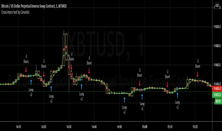
Cross impro test by Canundo Crossover Crossunder Tick valuesThis is a script where I tried to check the following things:
Even thought the tick of an asset is, for example 0.5, there are calculated prices, like SMA's that have even more decimals. Leading to crosses happening that for example happen at the same price. Consequently triggering totally useless in side markets. What happens if SMA values are restricted to the tick resolution? (Option works on it's own or with a combination of the others.)
What happens if I set my own tick value, like 0.8 instead of 0.5, what will be the effect for calculated values that are used for crossings? Will tick sizes improve the success rate? (This option will work only when the first option is active.)
Can success rate, especially for sideway markets be improved when adding a spread between MA's, so that it triggers less in sideway markets? (Option works on it's own or with a combination of the others.)
First of all, I had a hard time to round prices properly when it needs to be dynamic and working for different assets with different amounts of decimal values in the tick. The solution is that abs(floor(syminfo.mintick)) will give you the amount of decimals a tick has. It works for all ticks that are at least lower than 10. I'm not sure how huge ticks are out there. I did not implement this solution at the end since I found another way to test it.
Findings:
The first option, when activated, takes out half the trades and raises the percent profitability by 8% so there is some effect. However, all of the tested options have less advantage than I hoped for but are nevertheless something worthy for sideway markets. The first option just forces the MA's from the example to use the tick resolution.
See these two images. One when the first option is off, the second when it's active.
The lines are the MA's with adjusted values, the crosses are the places of the MA's when left as is.
Here a screenshot of the third option set to the value 2 on the 1 minute XBTUSD chart.
The advantage is that less trades trigger that have a low change in price and so less trading fees will happen.
The disadvantage is that all options can implement some delay for a crossing since the crossing will trigger once a slightly bigger move into the direction was taken.
This test environment was not meant to be profitable but to test the effects.
Maybe someone finds it interesting or wanted to test the same, so here you can save some work.
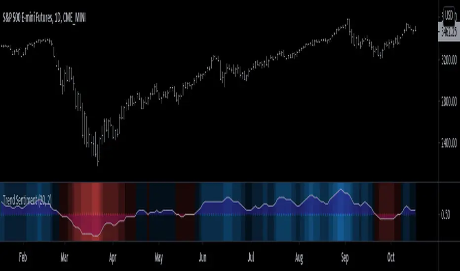
Trend Sentiment [racer8]Trend Sentiment is a trend indicator with enhanced graphics, that is, it has many different shades of blue and red.
The brighter the blue, the more bullish.
The brighter the red, the more bearish.
It is a simple indicator with a basic formula:
a = close > prev.close? ---> If yes, a = 1, otherwise a = 0.
b = sma of a over n periods -----1st parameter, n...."Length"
c = sma of b over j periods ----- 2nd parmeter, j..."Smoothing"
plot (c)
Is c > 0.5? ---> If yes, background color = blue, otherwise red.
plot background color.
plot 0.5 as dotted midline.
The Trend Sentiment value represents the percentage of bullish force in the market.
Signals are generated when it crosses the 50% mark.
Values above 0.50 are bullish and values below 0.50 are bearish.
Enjoy and hit the like button :)
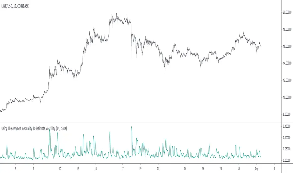
Using The AM/GM Inequality To Estimate VolatilityA volatility indicator derived from the AM/GM inequality. I don't think it will be necessary to describe the usage and interpretation of such indicator, and I don't think it is super useful, however, this is not the case of the script, which contains three ways to compute the geometric mean, with a classic, a simple, and an efficient way. The AM/GM inequality is also a really interesting concept, and I'll try to"prove" it in this post by using DSP. I also added more comments in the script in order to highlight some stuff.
The AM/GM Inequality
When we talk about the mean, we are referring to the "arithmetic" one by default, but there exist more types of means. Two other ones include the "geometric" and "harmonic" means, both are part of the Pythagorean means with the arithmetic mean.
Each one of them as several properties, but the most interesting aspect is their inequality, that is:
HM <= GM <= AM
The arithmetic mean is the one with the highest value, while the harmonic mean is the one with the lowest value. In the case each data point is equal to each other, all the means have the same value.
In our case, the inequality of interest is the inequality between the geometric and arithmetic mean, where the geometric mean is lower or equal than the arithmetic one. Many proofs/explanations exist, I'll try my version using DSP, where instead of thinking about means, we think about rolling means, which allows us to interpret them as low-pass filters. So we end up having the geometric moving average (GMA) and arithmetic moving average (SMA).
We know that GMA <= SMA , the SMA has a unity passband, this implies that the GMA has a passband lower than 1 (for non-equal input values), this explains why the GMA is smaller than the SMA. In order for a FIR filter to have a passband lower than 1, the sum of the filter coefficients must be lower than 1. In order to further proves this consider the following equation:
sqrt(a×b) = k×a + k×b
Here sqrt(a×b) is the geometric mean of a and b , the right-hand side of the equation is a weighted sum between a and b and coefficient k , we want to solve the equation with respect to k , if k×2 < 1 then we have the proof that GMA < SMA . The solution with respect to k is:
k = sqrt(a×b)/(a+b)
which always gives a number lower than 0.5, as such k×2 < 1 and thus the passband is lower than 1. If our input values are equal to each other, we end up with the following solution for k :
k = sqrt(a×a)/(a+a) = a/(2×a) = 0.5
as such the GMA has the coefficients of an SMA as long as the input values are equal to each other.
Because of this inequality, we can subtract the SMA to a GMA and take the square root of the result in order to have a volatility indicator, however, both moving averages are still pretty close to each other, which gives a very small result for the indicator.
Uwu I am a bit tired, better indicators coming up
Grid Like StrategyIt is possible to use progressive position sizing in order to recover from past losses, a well-known position sizing system being the "martingale", which consists of doubling your position size after a loss, this allows you to recover any previous losses in a losing streak + winning an extra. This system has seen a lot of attention from the trading community (mostly from beginners), and many strategies have been designed around the martingale, one of them being "grid trading strategies".
While such strategies often shows promising results on paper, they are often subjects to many frictions during live trading that makes them totally unusable and dangerous to the trader. The motivations behind posting such a strategy isn't to glorify such systems, but rather to present the problems behind them, many users come to me with their ideas and glorious ways to make money, sometimes they present strategies using the martingale, and it is important to present the flaws of this methodology rather than blindly saying "you shouldn't use it".
Strategy Settings
Point determines the "grid" size and should be adjusted accordingly to the scale of the symbol you are applying the strategy to. Higher value would require larger price movements in order to trigger a trade, as such higher values will generate fewer trades.
The order size determines the number of contracts/shares to purchase.
The martingale multiplier determines the factor by which the position size is multiplied after a loss, using values higher to 2 will "squarify" your balance, while a value of 1 would use a constant position sizing.
Finally, the anti-martingale parameter determines whether the strategy uses a reverse martingale or not, if set to true then the position size is multiplied after any wins.
The Grid
Grid strategies are commons and do not present huge problems until we use certain position sizing methods such as the martingale. A martingale is extremely sensitive to any kind of friction (frictional costs, slippage...etc), the grid strategy aims to provide a stable and simple environment where a martingale might possibly behave well.
The goal of a simple grid strategy is to go long once the price crossover a certain level, a take profit is set at the level above the current one and stop loss is placed at the level below the current one, in a winning scenario the price reach the take profit, the position is closed and a new one is opened with the same setup. In a losing scenario, the price reaches the stop loss level, the position is closed and a short one is opened, the take profit is set at the level below the current one, and a stop loss is set at the level above the current one. Note that all levels are equally spaced.
It follows from this strategy that wins and losses should be constant over time, as such our balance would evolve in a linear fashion. This is a great setup for a martingale, as we are theoretically assured to recover all the looses in a losing streak.
Martingale - Exponential Decays - Risk/Reward
By using a martingale we double our position size (exposure) each time we lose a trade, if we look at our balance when using a martingale we see significant drawdowns, with our balance peaking down significantly. The martingale sequence is subject to exponential growth, as such using a martingale makes our balance exposed to exponential decays, that's really bad, we could basically lose all the initially invested capital in a short amount of time, it follows from this that the theoretical success of a martingale is determined by what is the maximum losing streak you can endure
Now consider how a martingale affects our risk-reward ratio, assuming unity position sizing our martingale sequence can be described by 2^(x-1) , using this formula we would get the amount of shares/contracts we need to purchase at the x trade of a losing streak, we would need to purchase 256 contracts in order to recover from a losing streak of size 9, this is enormous when you take into account that your wins are way smaller, the risk-reward ratio is totally unfair.
Of course, some users might think that a losing streak of size 9 is pretty unlikely, if the probability of winning and losing are both equal to 0.5, then the probability of 9 consecutive losses is equal to 0.5^9 , there are approximately 0.2% of chance of having such large losing streak, note however that under a ranging market such case scenario could happen, but we will see later that the length of a losing streak is not the only problem.
Other Problems
Having a capital large enough to tank 9any number of consecutive losses is not the only thing one should focus on, as we have to take into account market prices and trading dynamics, that's where the ugly part start.
Our first problem is frictional costs, one example being the spread, but this is a common problem for any strategy, however here a martingale is extra sensitive to it, if the strategy does not account for it then we will still double our positions costs but we might not recover all the losses of a losing streak, instead we would be recovering only a proportion of it, under such scenario you would be certain to lose over time.
Another problem are gaps, market price might open under a stop-loss without triggering it, and this is a big no-no.
Equity of the strategy on AMD, in a desired scenario the equity at the second arrow should have been at a higher position than the equity at the first arrow.
In order for the strategy to be more effective, we would need to trade a market that does not close, such as the cryptocurrency market. Finally, we might be affected by slippage, altho only extreme values might drastically affect our balance.
The Anti Martingale
The strategy lets you use an anti-martingale, which double the position size after a win instead of a loss, the goal here is not to recover from a losing strike but instead to profit from a potential winning streak.
Here we are exposing your balance to exponential gross but you might also lose a trade at the end a winning streak, you will generally want to reinitialize your position size after a few wins instead of waiting for the end of a streak.
Alternative
You can use other-kind of progressions for position sizing, such as a linear one, increasing your position size by a constant number each time you lose. More gentle progressions will recover a proportion of your losses in a losing streak.
You can also simulate the effect of a martingale without doubling your position size by doubling your target profit, if for example you have a 10$ profit-target/stop-loss and lose a trade, you can use a 20$ profit target to recover from the lost trade + gain a profit of 10$. While this approach does not introduce exponential decay in your balance, you are betting on the market reaching your take profits, considering the fact that you are doubling their size you are expecting market volatility to increase drastically over time, as such this approach would not be extremely effective for high losing streak.
Conclusion
You will see a lot of auto-trading strategies that are based on a grid approach, they might even use a martingale. While the backtests will look appealing, you should think twice before using such kind of strategy, remember that frictional costs will be a huge challenge for the strategy, and that it assumes that the trader has an important initial capital. We have also seen that the risk/reward ratio is theoretically the worst you can have on a strategy, having a low reward and a high risk. This does not mean that progressive position sizing is bad, but it should not be pushed to the extreme.
It is nice to note that the martingale is originally a betting system designed for casino games, which unlike trading are not subject to frictional costs, but even casino players don't use it, so why would you?
Thx for reading

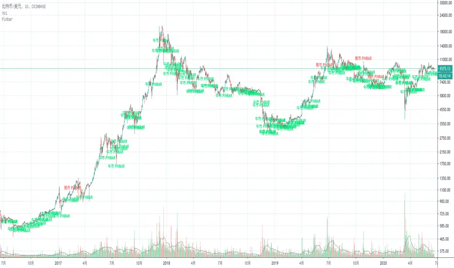
Pinbar识别器This is a Pinbar Monitor which design for Chinese.
这是一个Pinbar识别器。
本脚本的目的在于帮助使用中文的人了解该指标,特别是其用法。同时将该指标代码添加完整的中文注释,方便使用中文的人学习Pine语言。
Pinbar概念来自于Price Action,基本类似于国内K线分析中的十字星,锤子线。该指标的主要功用在于帮助识别盘面出现的Pinbar,分为牛市Pinbar和熊市Pinbar。
对Pinbar的量化定义
熊市Pinbar
1 前一根K线,必须为阳线;
2 K线实体必须小于前一根K线;
3 下影线高度至少大于0.5倍实体高度;
4 上影线高度至少是2倍实体高度。
牛市Pinbar
1 前一根K线,必须为阴线;
2 K线实体必须小于前一根K线;
3 上影线高度至少大于0.5倍实体高度;
4 下影线高度至少是2倍实体高度。
指标局限性
因为Pinbar出现的概率比较高,所以切勿直接按信号交易,应考虑其他的分析方法,综合考虑再决定是否交易。
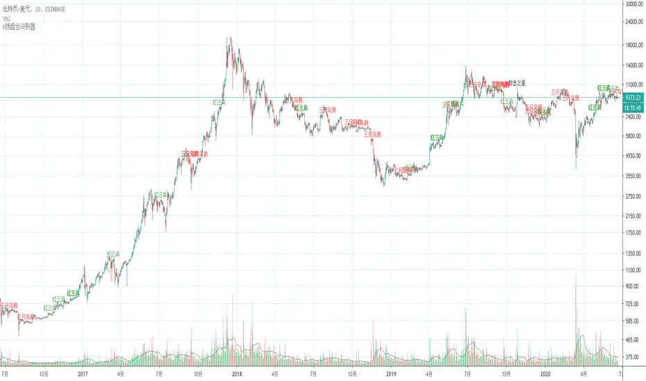
K线组合识别器(Candlestick Pattern Monitor)This is a Candlestick Pattern Monitor which design for Chinese.
这是一个K线组合的识别器。
本脚本的目的在于帮助使用中文的人了解该指标,特别是其用法。同时将该指标代码添加完整的中文注释,方便使用中文的人学习Pine语言。
K线组合是国内技术分析里最常见的分析方式之一。K线组合种类丰富,各类证券类书籍中均有总结,本识别器选取其中几种传播度最高几个K线组合,将其量化,使用机器辅助识别K线组合。
射击之星
射击之星,在股价运行的高位,一根中阳或者大阳线之后出现长上影K线,往往是较为强烈的看空信号,K线的实体部分很小或者为十字线,上影线一般为实体K线的两倍以上。
量化要点:
1 上一根K线须是一根实体高度必须大于最近10根K线实体平均值1.5倍;
2 上影线至少是实体的2倍;
3 下影线不大于实体的0.5倍。
乌云盖顶
乌云盖顶组合,第一根K线为大阳线或者中阳线,第二天跳空高开,第二根K线的开盘价远高于第一根K线的最高价,但是收盘却跌入第一根K线的实体部分,第二根K线收盘价越底,则拐点的信号越明确。
量化要点:
1 跳开,即当前K线开盘价大于上一根收盘价;
2 上一根K线须是一根实体高度必须大于最近10根K线实体平均值1.5倍;
3 当前K线收于前一根K线实体下半部分。
三只乌鸦
三只乌鸦组合的构成,股价上涨的高位区域,一根大阳线之后连续出现三根小阴线,每一根阴线都是跳空高开,但是收在当日最低附近。
量化要点:
1 连续三根阴线;
2 三根阴线的实体都小于最近十根K线实体的平均值。
下跌三部曲
下跌三部曲的构成,一根大阴线或者中阴线之后,随后的交易日连续三根价量逐日萎缩的小阳线,三根小阳线的最高价未能击破前面阴线的开盘价,随即股价重回下跌趋势,并再报收大阴线或者中阴线。
量化要点:
1 组合第一根K线为阴线;
2 组合的第二至第四根K线都为阳线;
3 第四根K线收盘价不高于第一根K线开盘价;
4 第五根K线为阴线,且收盘价低于第二根K线开盘价。
早晨之星
早晨之星由三根K线组合成,第一根是中阴线或者大阴线,第二根是小阳线或者小阴线,第三根为中阳线或者大阳线,如果第二根是十字线,也成为早晨之星,第三根阳线实体切入第一根阴线的实体之内,切入的幅度越大,信号越明确。
量化要点:
1 第一根K线为阴线,且实体高度大于最近十根K线实体的平均值的1.5倍;
2 第二根K线实体高度小于最近十根K线实体的平均值,且上影线小于实体的0.5倍,下影线大于实体的2倍;
3 第三根K线为阳线,且收盘价大于第一根K线开盘价。
红三兵
红三兵构成,三根上涨的小阳K线,如果出现在大跌之后的底部区域或者盘整区域,再配合成交量,往往成为上涨行情的先兆。
量化要点:
1 三根K线均为阳线;
2 三根K线的实体均小于最近十根K线实体的平均值。
指标局限性
因K线组合出现的频次均较高,所以K线组合需结合其他分析方式一起考虑。
Hashem Correlation CoefficientCorrelation Coefficient
Core Code from: www.tradingview.com
This indicator Show Correlation between the Current Ticker & timeframe and a Customizable Ticker. After adding the indicator you can change the second ticker in the settings.
The Correlation Coeff is between -1 to 1 which 1 means 100% correlation and -1 means -100% correlation ( Inverse Correlation ).
The color of the area changes when:
Blue : CC > 0.5
Aqua : CC > 0.75
Purple : CC < -0.5
Red : CC < -0.75
Hancock - IFT RSI T3MAThis is a version of the Inverse Fisher Transform Relative Strength Index with T3MA smoothing and histogram difference based on EMA signal line.
Configurable parameters:
RSI length - This is the period used for the RSI .
RSI Smooth Length - This is the smoothing period of the Weighted Moving Average used for the smoothing in Inverse Fisher Transform .
RSI Signal - This is the period used for EMA signal line.
RSI Overbought - Configures the overbought threshold (0.5 default).
RSI Oversold - Configures the oversold threshold (-0.5 default).
T3 Smoothing - Enabling this applies T3MA smoothing to the RSI .
T3 Length - This is the period used for the T3MA smoothing of the RSI .
T3 Factor - This is the factor used for the T3MA smoothing of the RSI .
I've added a histogram plotting the difference between the signal line and RSI to make it easier to make trades. Oversold and Overbought thresholds are indicated by the red and green horizontal lines. Signal line is coloured for trade direction.
Happy trading folks!
Hancock

CPR WidthThe indicator shows the width of the Central Pivot Range. Frank Ochoa call it It Pivot Range Histogram in his book.
Use it in conjunction with the Central Pivot Range indicator.
Below is the interpretation of the reading.
CPR Width > 0.5 - Sideways or Trading Range Day,
CPR Width > 0.75 - increases the likelihood of sideways trading behavior,
CPR Width < 0.5 - Trending type of day,
CPR Width < 0.25 - increases the likelihood of a trending market.
The above reading only increases the likely-hood of the possibility and not always right.

Powered Kaufman Adaptive Moving AverageIntroduction
The ability the Kaufman adaptive moving average (KAMA) has to be flat during ranging markets and close to the price during trending markets is what make this moving average one of the most useful in technical analysis. KAMA is calculated by using exponential averaging using the efficiency ratio (ER) as smoothing variable where 1 > ER > 0 . An increasing efficiency ratio indicate a trending market. Based on one of my latest indicator (see Kaufman Adaptive Bands) i propose this modified KAMA that allow to emphasis the abilities of KAMA by powering the efficiency ratio. I also added a new option that allow for even more adaptivity.
The Indicator
The indicator is a simple KAMA of period length that use a powered ER with exponent factor .
When factor = 1 the indicator is a simple KAMA, however when factor > 1 there can be more emphasis on the flattening effect of KAMA.
You can also restrain this effect by using 1 > factor > 0
Note that when the exponent is lower than 1 and greater than 0 you are basically applying a nth square root to the value, for example pow(2,0.5) = sqrt(2) because 1/0.5 = 2, in our case :
pow(ER,factor > 1) < ER and pow(ER,1 > factor > 0) > ER
Self Powered P-KAMA
When the self powered option is checked you are basically powering ER with the reciprocal of ER as exponent, however factor does no longer change anything. This can give interesting results since the exponent depend on the market trend strength.
In orange the self powered KAMA of period length = 50 and in blue a basic powered KAMA with a factor of 3 and a period of length = 50.
Conclusion
Applying basic math to indicators is always fun and easy to do, if you have adaptive moving averages using exponential averaging try powering your smoothing variable in order to see interesting results. I hope you like this indicator. Thanks for reading !

RVOL - Final on 814 for 3m Candles ONLYRelative Volume for 3 minute charts ONLY.
Lookback 20 days.
Historical and average values are used to formulate the ratio.
Thank you to R4Rocket for the initial code.
I also researched the RVOL output in Trade Ideas to align the final ratio as close as possible.
The colors change at different levels:
<0.5 ; Red
0.5 > and <=.65 ; Orange
0.65 > and <=1 ; Dark Yellow
1 > and <=1.25 ; Bright Yellow
1.25 < and <=1.5 ; Dark Green
1.5 < and <=2 ; Brighter Green
Above 2 ; Very Bright Green

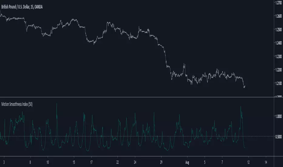
Motion Smoothness Index Introduction
Its holiday time for me, i have been working here a lot. But no leaving before publishing. Telling when market price is smooth or rough is not the easiest task, so today i present a trend metric indicator that allow you to give you this kind of information.
The Indicator
The indicator is in an approximate range of (0,1) with mean x̄ decaying for higher length's, when the indicator is below 0.5 the market is smooth, else rough, this is the simple interpretation. The indicator is simply the ratio of the price residual standard deviation and the price standard deviation.
Higher value of length will make the indicator less accurate when it comes to detect rough market price, you can still use the indicator direction or its running mean to give you insights but 0.5 is still the recommended detection threshold.
In More Depth
Even tho market is random by nature there can still be structures in the price (cycles and trends), the fractional BM model will tell you that market price is sometimes auto-correlated (trending) or non auto-correlated (ranging), knowing what is the current market state is therefore important, when price is rough it can means an excess in noise thus exhibiting an uncorrelated market at the contrary of a smoother price that can allow for auto-correlation.
Now, market is infected by noise, and thats really unfortunate but the noise posses various properties that can allow for all the structures we see in market price. So thinking about the market allowing for possible profits during auto-correlated states is encouraging.
Conclusion
Although the indicator measure smoothness/roughness it can still be interpreted as a trend/range state detector. I hope it provide to be useful.
I wish you all good holidays and see you next time ! Thanks for reading !
Time Price IndicatorIntroduction
There are already several indicators who measure the time behavior relative to price, the most well know being the Aroon indicator published by Tushar Chande. I propose an alternative indicator TPI who tend to create less whipsaw's at the cost of small reactivity.
The Indicator
The TPI is in a range of 0.5/-0.5 and is no different than the Aroon indicator when it come to signal generation, when the upper line (in blue) crossover the lower line (in orange) the indicator generate a buy signal, when the lower line cross under the upper line a sell signal is generated.
Comparison
The Aroon indicator tend to use more information which involve more reactivity but more uncertainty as well.
Aroon and TPI with both length = 50. White lines represent signals where the Aroon and my proposed indicator react at the same time, the red line show a whipsaw and the green line show a signal generated faster by the Aroon.
Here is a more pertinent exemple
Aroon reacted to price range which at the end involved many whipsaw, the TPI however stayed on a sell signal and did not reacted to this price range. The cost to avoid so many whipsaw was a reactivity of 7 bars back when the sell signal of the TPI was generated.
A statistic of the signal numbers generated by both indicator is shown below
The blue line show the number of signals generated by the Aroon indicator and in orange the number generated by the TPI with both length = 14. Aroon generated 410 while the TPI generated 288 signals.
Conclusion
The Aroon indicator and TPI can both generate a signal at the same time or with a small period deviation with the ability of the TPI to avoid some whipsaw.

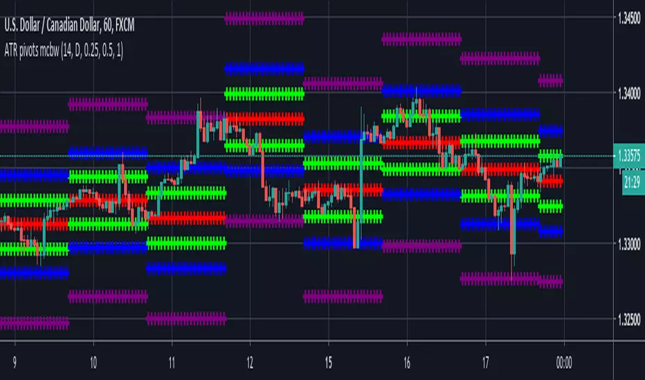
ATR based Pivots mcbwHey everyone this is an exciting new script I have prepared for you.
I was reading an old forex bulletin article some time ago when I came across this: solar.murty.net (or you can download the full bulletin with lots of other good articles here: www.forexfactory.com).
You can already buy this for metatrader (www.mql5.com) so I figured to make it for free for tradingview.
This bulletin suggested that you can reasonably predict daily volatility by adding or subtracting multiples of the daily ATR to the daily opening. Using this you can choose multiples to use as price targets and alternatively as stop losses. For example, if you already have a sense of market direction you can buy at market open place a stop loss at - 1 daily ATR and a profit target at + 3 ATRs for a risk to reward ratio of 3. If you are looking for smaller/quicker moves with a ratio of 3 you can have a stop loss at -0.25 ATR and a take profit at +0.75 ATR.
Alternatively this article also suggests to use this method to catch volatility breakouts. If price is higher than the + 1 ATR area then you can safely assume it will be going to the +2 ATR area so you can put a buy stop at + 1 ATR with a profit target at + 2 ATR with a stop loss at +0.5 ATR to catch a volatility breakout with a risk to reward ratio of 2!
Even further there are methods that you can use with ATRs of multiple window sizes, for example by opening two copies of this indicator and measuring recent volatility with a 1 week window and long term volatility within a 1 month window. If the short term volatility is crossing the long term volatility then there is a high probability chance that even more price movement will occur.
However I have found that this method is good for more than daily volatility , it can also be used to measure weekly volatility , and monthly volatility and use these multiples as good long term price targets.
To select if you want daily, weekly, or monthly values of the ATR of volatility you're using go to the settings and click on the options in the "Opening period". The default window of the ATR here is 14 periods, but you can change this if you want to in "ATR period". Most importantly you are able to select which multiples of the ATR you would like to use in the settings in "ATR multiple 1" which is the green line, "ATR multiple 2" which is the blue line, and "ATR multiple 3" which is the purple line. You can select any values you want to put in these, the choice of 0.25, 0.5, and 1 is not special, some people use fibonacci numbers here or simply 0.33, 0.66, and 0.99.
Repainting issue: This script uses the daily value of the Average True Range (ATR), which measures the volatility that is happening today. If price becomes more volatile then the value of the ATR can increase throughout the day, but it can never decrease. What this means is that the ATR based pivots are able to expand away from the opening price, which should not affect the trades that you take based on these areas. If you base your take profit on one of these ATR multiples and the daily volatility increase this means that your take profit area will be closer to your entry than the ATR multiple. Meaning that your trades will be more conservative.
While this all may sound very technical it is super intuitive, throw this on your chart and play around with it :)
Happy trading!
General Filter Estimator-An Experiment on Estimating EverythingIntroduction
The last indicators i posted where about estimating the least squares moving average, the task of estimating a filter is a funny one because its always a challenge and it require to be really creative. After the last publication of the 1LC-LSMA , who estimate the lsma with 1 line of code and only 3 functions i felt like i could maybe make something more flexible and less complex with the ability to approximate any filter output. Its possible, but the methods to do so are not something that pinescript can do, we have to use another base for our estimation using coefficients, so i inspired myself from the alpha-beta filter and i started writing the code.
Calculation and The Estimation Coefficients
Simplicity is the key word, its also my signature style, if i want something good it should be simple enough, so my code look like that :
p = length/beta
a = close - nz(b ,close)
b = nz(b ,close) + a/p*gamma
3 line, 2 function, its a good start, we could put everything in one line of code but its easier to see it this way. length control the smoothing amount of the filter, for any filter f(Period) Period should be equal to length and f(Period) = p , it would be inconvenient to have to use a different length period than the one used in the filter we want to estimate (imagine our estimation with length = 50 estimating an ema with period = 100) , this is where the first coefficients beta will be useful, it will allow us to leave length as it is. In general beta will be greater than 1, the greater it will be the less lag the filter will have, this coefficient will be useful to estimate low lagging filters, gamma however is the coefficient who will estimate lagging filters, in general it will range around .
We can get loose easily with those coefficients estimation but i will leave a coefficients table in the code for estimating popular filters, and some comparison below.
Estimating a Simple Moving Average
Of course, the boxcar filter, the running mean, the simple moving average, its an easy filter to use and calculate.
For an SMA use the following coefficients :
beta = 2
gamma = 0.5
Our filter is in red and the moving average in white with both length at 50 (This goes for every comparison we will do)
Its a bit imprecise but its a simple moving average, not the most interesting thing to estimate.
Estimating an Exponential Moving Average
The ema is a great filter because its length times more computing efficient than a simple moving average. For the EMA use the following coefficients :
beta = 3
gamma = 0.4
N.B : The EMA is rougher than the SMA, so it filter less, this is why its faster and closer to the price
Estimating The Hull Moving Average
Its a good filter for technical analysis with tons of use, lets try to estimate it ! For the HMA use the following coefficients :
beta = 4
gamma = 0.85
Looks ok, of course if you find better coefficients i will test them and actualize the coefficient table, i will also put a thank message.
Estimating a LSMA
Of course i was gonna estimate it, but this time this estimation does not have anything a lsma have, no moving average, no standard deviation, no correlation coefficient, lets do it.
For the LSMA use the following coefficients :
beta = 3.5
gamma = 0.9
Its far from being the best estimation, but its more efficient than any other i previously made.
Estimating the Quadratic Least Square Moving Average
I doubted about this one but it can be approximated as well. For the QLSMA use the following coefficients :
beta = 5.25
gamma = 1
Another ok estimate, the estimate filter a bit more than needed but its ok.
Jurik Moving Average
Its far from being a filter that i like and its a bit old. For the comparison i will use the JMA provided by @everget described in this article : c.mql5.com
For the JMA use the following coefficients :
for phase = 0
beta = pow*2 (pow is a parameter in the Jma)
gamma = 0.5
Here length = 50, phase = 0, pow = 5 so beta = 10
Looks pretty good considering the fact that the Jma use an adaptive architecture.
Discussion
I let you the task to judge if the estimation is good or not, my motivation was to estimate such filters using the less amount of calculations as possible, in itself i think that the code is quite elegant like all the codes of IIR filters (IIR Filters = Infinite Impulse Response : Filters using recursion) .
It could be possible to have a better estimate of the coefficients using optimization methods like the gradient descent. This is not feasible in pinescript but i could think about it using python or R.
Coefficients should be dependant of length but this would lead to a massive work, the variation of the estimation using fixed coefficients when using different length periods is just ok if we can allow some errors of precision.
I dont think it should be possible to estimate adaptive filter relying a lot on their adaptive parameter/smoothing constant except by making our coefficients adaptive (gamma could be)
So at the end ? What make a filter truly unique ? From my point of sight the architecture of a filter and the problem he is trying to solve is what make him unique rather than its output result. If you become a signal, hide yourself into noise, then look at the filters trying to find you, what a challenging game, this is why we need filters.
Conclusion
I wanted to give a simple filter estimator relying on two coefficients in order to estimate both lagging and low-lagging filters. I will try to give more precise estimate and update the indicator with new coefficients.
Thanks for reading !