Komut dosyalarını "用户自选股中各股票的均线排列状态(5日、10日、20日均线)" için ara
Adv EMA Cloud v6 (ADX, Alerts)Summary:
This indicator provides a multi-faceted view of market trends using Exponential Moving Averages (EMAs) arranged in visually intuitive clouds, enhanced with an optional ADX-based range filter and configurable alerts for key market conditions. It aims to help traders quickly gauge trend alignment across short, medium, and long timeframes while filtering signals during potentially choppy market conditions.
Key Features:
Multiple EMAs: Displays 10-period (Fast), 20-period (Mid), and 50-period (Slow) EMAs.
Long-Term Trend Filter: Includes a 200-period EMA to provide context for the overall dominant trend direction.
Dual EMA Clouds:
Fast/Mid Cloud (10/20 EMA): Fills the area between the 10 and 20 EMAs. Defaults to Green when 10 > 20 (bullish short-term momentum) and Red when 10 < 20 (bearish short-term momentum).
Mid/Slow Cloud (20/50 EMA): Fills the area between the 20 and 50 EMAs. Defaults to Aqua when 20 > 50 (bullish mid-term trend) and Fuchsia when 20 < 50 (bearish mid-term trend).
Optional ADX Range Filter: Uses the Average Directional Index (ADX) to identify potentially non-trending or choppy markets. When enabled and ADX falls below a user-defined threshold, the EMA clouds will turn grey, visually warning that trend-following signals may be less reliable.
Configurable Alerts: Provides several built-in alert conditions using Pine Script's alertcondition function:
Confluence Condition: Triggers when a 10/20 EMA crossover occurs while both EMA clouds show alignment (both bullish/green/aqua or both bearish/red/fuchsia) and price respects the 200 EMA filter and the ADX filter indicates a trend (if filters are enabled).
MA Filter Cross: Triggers when price crosses above or below the 200 EMA filter line.
Full Alignment Start: Triggers on the first bar where full bullish or bearish alignment occurs (both clouds aligned + MA filter respected + ADX trending, if filters are enabled).
How It Works:
EMA Calculation: Standard Exponential Moving Averages are calculated for the 10, 20, 50, and 200 periods based on the closing price.
Cloud Creation: The fill() function visually shades the area between the 10 & 20 EMAs and the 20 & 50 EMAs.
Cloud Coloring: The color of each cloud is determined by the relationship between the two EMAs that define it (e.g., if EMA 10 is above EMA 20, the first cloud is bullish-colored).
ADX Filter Logic: The script calculates the ADX value. If the "Use ADX Trend Filter?" input is checked and the calculated ADX is below the specified "ADX Trend Threshold", the script considers the market potentially ranging.
ADX Visual Effect: During detected ranging periods (if the ADX filter is active), the plotCloud12Color and plotCloud23Color variables are assigned a neutral grey color instead of their normal bullish/bearish colors before being passed to the fill() function.
Alert Logic: Boolean variables track the specific conditions (crossovers, cloud alignment, filter positions, ADX state). The alertcondition() function creates triggerable alerts based on these pre-defined conditions.
Potential Interpretation (Not Financial Advice):
Trend Alignment: When both clouds share the same directional color (e.g., both bullish - Green & Aqua) and price is on the corresponding side of the 200 EMA filter, it may suggest a stronger, more aligned trend. Conversely, conflicting cloud colors may indicate indecision or transition.
Dynamic Support/Resistance: The EMA lines themselves (especially the 20, 50, and 200) can sometimes act as dynamic levels where price might react.
Range Warning: Greyed-out clouds (when ADX filter is enabled) serve as a visual warning that trend-based strategies might face increased difficulty or whipsaws.
Confluence Alerts: The specific confluence alerts signal moments where multiple conditions align (crossover + cloud agreement + filters), which some traders might view as higher-probability setups.
Customization:
All EMA lengths (10, 20, 50, 200) are adjustable via the Inputs menu.
The ADX length and threshold are configurable.
The MA Trend Filter and ADX Trend Filter can be independently enabled or disabled.
Disclaimer:
This indicator is provided for informational and educational purposes only. Trading financial markets involves significant risk. Past performance is not indicative of future results. Always conduct your own thorough analysis and consider your risk tolerance before making any trading decisions. This indicator should be used in conjunction with other analysis methods and tools. Do not trade based solely on the signals or visuals provided by this indicator.

Tensor Market Analysis Engine (TMAE)# Tensor Market Analysis Engine (TMAE)
## Advanced Multi-Dimensional Mathematical Analysis System
*Where Quantum Mathematics Meets Market Structure*
---
## 🎓 THEORETICAL FOUNDATION
The Tensor Market Analysis Engine represents a revolutionary synthesis of three cutting-edge mathematical frameworks that have never before been combined for comprehensive market analysis. This indicator transcends traditional technical analysis by implementing advanced mathematical concepts from quantum mechanics, information theory, and fractal geometry.
### 🌊 Multi-Dimensional Volatility with Jump Detection
**Hawkes Process Implementation:**
The TMAE employs a sophisticated Hawkes process approximation for detecting self-exciting market jumps. Unlike traditional volatility measures that treat price movements as independent events, the Hawkes process recognizes that market shocks cluster and exhibit memory effects.
**Mathematical Foundation:**
```
Intensity λ(t) = μ + Σ α(t - Tᵢ)
```
Where market jumps at times Tᵢ increase the probability of future jumps through the decay function α, controlled by the Hawkes Decay parameter (0.5-0.99).
**Mahalanobis Distance Calculation:**
The engine calculates volatility jumps using multi-dimensional Mahalanobis distance across up to 5 volatility dimensions:
- **Dimension 1:** Price volatility (standard deviation of returns)
- **Dimension 2:** Volume volatility (normalized volume fluctuations)
- **Dimension 3:** Range volatility (high-low spread variations)
- **Dimension 4:** Correlation volatility (price-volume relationship changes)
- **Dimension 5:** Microstructure volatility (intrabar positioning analysis)
This creates a volatility state vector that captures market behavior impossible to detect with traditional single-dimensional approaches.
### 📐 Hurst Exponent Regime Detection
**Fractal Market Hypothesis Integration:**
The TMAE implements advanced Rescaled Range (R/S) analysis to calculate the Hurst exponent in real-time, providing dynamic regime classification:
- **H > 0.6:** Trending (persistent) markets - momentum strategies optimal
- **H < 0.4:** Mean-reverting (anti-persistent) markets - contrarian strategies optimal
- **H ≈ 0.5:** Random walk markets - breakout strategies preferred
**Adaptive R/S Analysis:**
Unlike static implementations, the TMAE uses adaptive windowing that adjusts to market conditions:
```
H = log(R/S) / log(n)
```
Where R is the range of cumulative deviations and S is the standard deviation over period n.
**Dynamic Regime Classification:**
The system employs hysteresis to prevent regime flipping, requiring sustained Hurst values before regime changes are confirmed. This prevents false signals during transitional periods.
### 🔄 Transfer Entropy Analysis
**Information Flow Quantification:**
Transfer entropy measures the directional flow of information between price and volume, revealing lead-lag relationships that indicate future price movements:
```
TE(X→Y) = Σ p(yₜ₊₁, yₜ, xₜ) log
```
**Causality Detection:**
- **Volume → Price:** Indicates accumulation/distribution phases
- **Price → Volume:** Suggests retail participation or momentum chasing
- **Balanced Flow:** Market equilibrium or transition periods
The system analyzes multiple lag periods (2-20 bars) to capture both immediate and structural information flows.
---
## 🔧 COMPREHENSIVE INPUT SYSTEM
### Core Parameters Group
**Primary Analysis Window (10-100, Default: 50)**
The fundamental lookback period affecting all calculations. Optimization by timeframe:
- **1-5 minute charts:** 20-30 (rapid adaptation to micro-movements)
- **15 minute-1 hour:** 30-50 (balanced responsiveness and stability)
- **4 hour-daily:** 50-100 (smooth signals, reduced noise)
- **Asset-specific:** Cryptocurrency 20-35, Stocks 35-50, Forex 40-60
**Signal Sensitivity (0.1-2.0, Default: 0.7)**
Master control affecting all threshold calculations:
- **Conservative (0.3-0.6):** High-quality signals only, fewer false positives
- **Balanced (0.7-1.0):** Optimal risk-reward ratio for most trading styles
- **Aggressive (1.1-2.0):** Maximum signal frequency, requires careful filtering
**Signal Generation Mode:**
- **Aggressive:** Any component signals (highest frequency)
- **Confluence:** 2+ components agree (balanced approach)
- **Conservative:** All 3 components align (highest quality)
### Volatility Jump Detection Group
**Volatility Dimensions (2-5, Default: 3)**
Determines the mathematical space complexity:
- **2D:** Price + Volume volatility (suitable for clean markets)
- **3D:** + Range volatility (optimal for most conditions)
- **4D:** + Correlation volatility (advanced multi-asset analysis)
- **5D:** + Microstructure volatility (maximum sensitivity)
**Jump Detection Threshold (1.5-4.0σ, Default: 3.0σ)**
Standard deviations required for volatility jump classification:
- **Cryptocurrency:** 2.0-2.5σ (naturally volatile)
- **Stock Indices:** 2.5-3.0σ (moderate volatility)
- **Forex Major Pairs:** 3.0-3.5σ (typically stable)
- **Commodities:** 2.0-3.0σ (varies by commodity)
**Jump Clustering Decay (0.5-0.99, Default: 0.85)**
Hawkes process memory parameter:
- **0.5-0.7:** Fast decay (jumps treated as independent)
- **0.8-0.9:** Moderate clustering (realistic market behavior)
- **0.95-0.99:** Strong clustering (crisis/event-driven markets)
### Hurst Exponent Analysis Group
**Calculation Method Options:**
- **Classic R/S:** Original Rescaled Range (fast, simple)
- **Adaptive R/S:** Dynamic windowing (recommended for trading)
- **DFA:** Detrended Fluctuation Analysis (best for noisy data)
**Trending Threshold (0.55-0.8, Default: 0.60)**
Hurst value defining persistent market behavior:
- **0.55-0.60:** Weak trend persistence
- **0.65-0.70:** Clear trending behavior
- **0.75-0.80:** Strong momentum regimes
**Mean Reversion Threshold (0.2-0.45, Default: 0.40)**
Hurst value defining anti-persistent behavior:
- **0.35-0.45:** Weak mean reversion
- **0.25-0.35:** Clear ranging behavior
- **0.15-0.25:** Strong reversion tendency
### Transfer Entropy Parameters Group
**Information Flow Analysis:**
- **Price-Volume:** Classic flow analysis for accumulation/distribution
- **Price-Volatility:** Risk flow analysis for sentiment shifts
- **Multi-Timeframe:** Cross-timeframe causality detection
**Maximum Lag (2-20, Default: 5)**
Causality detection window:
- **2-5 bars:** Immediate causality (scalping)
- **5-10 bars:** Short-term flow (day trading)
- **10-20 bars:** Structural flow (swing trading)
**Significance Threshold (0.05-0.3, Default: 0.15)**
Minimum entropy for signal generation:
- **0.05-0.10:** Detect subtle information flows
- **0.10-0.20:** Clear causality only
- **0.20-0.30:** Very strong flows only
---
## 🎨 ADVANCED VISUAL SYSTEM
### Tensor Volatility Field Visualization
**Five-Layer Resonance Bands:**
The tensor field creates dynamic support/resistance zones that expand and contract based on mathematical field strength:
- **Core Layer (Purple):** Primary tensor field with highest intensity
- **Layer 2 (Neutral):** Secondary mathematical resonance
- **Layer 3 (Info Blue):** Tertiary harmonic frequencies
- **Layer 4 (Warning Gold):** Outer field boundaries
- **Layer 5 (Success Green):** Maximum field extension
**Field Strength Calculation:**
```
Field Strength = min(3.0, Mahalanobis Distance × Tensor Intensity)
```
The field amplitude adjusts to ATR and mathematical distance, creating dynamic zones that respond to market volatility.
**Radiation Line Network:**
During active tensor states, the system projects directional radiation lines showing field energy distribution:
- **8 Directional Rays:** Complete angular coverage
- **Tapering Segments:** Progressive transparency for natural visual flow
- **Pulse Effects:** Enhanced visualization during volatility jumps
### Dimensional Portal System
**Portal Mathematics:**
Dimensional portals visualize regime transitions using category theory principles:
- **Green Portals (◉):** Trending regime detection (appear below price for support)
- **Red Portals (◎):** Mean-reverting regime (appear above price for resistance)
- **Yellow Portals (○):** Random walk regime (neutral positioning)
**Tensor Trail Effects:**
Each portal generates 8 trailing particles showing mathematical momentum:
- **Large Particles (●):** Strong mathematical signal
- **Medium Particles (◦):** Moderate signal strength
- **Small Particles (·):** Weak signal continuation
- **Micro Particles (˙):** Signal dissipation
### Information Flow Streams
**Particle Stream Visualization:**
Transfer entropy creates flowing particle streams indicating information direction:
- **Upward Streams:** Volume leading price (accumulation phases)
- **Downward Streams:** Price leading volume (distribution phases)
- **Stream Density:** Proportional to information flow strength
**15-Particle Evolution:**
Each stream contains 15 particles with progressive sizing and transparency, creating natural flow visualization that makes information transfer immediately apparent.
### Fractal Matrix Grid System
**Multi-Timeframe Fractal Levels:**
The system calculates and displays fractal highs/lows across five Fibonacci periods:
- **8-Period:** Short-term fractal structure
- **13-Period:** Intermediate-term patterns
- **21-Period:** Primary swing levels
- **34-Period:** Major structural levels
- **55-Period:** Long-term fractal boundaries
**Triple-Layer Visualization:**
Each fractal level uses three-layer rendering:
- **Shadow Layer:** Widest, darkest foundation (width 5)
- **Glow Layer:** Medium white core line (width 3)
- **Tensor Layer:** Dotted mathematical overlay (width 1)
**Intelligent Labeling System:**
Smart spacing prevents label overlap using ATR-based minimum distances. Labels include:
- **Fractal Period:** Time-based identification
- **Topological Class:** Mathematical complexity rating (0, I, II, III)
- **Price Level:** Exact fractal price
- **Mahalanobis Distance:** Current mathematical field strength
- **Hurst Exponent:** Current regime classification
- **Anomaly Indicators:** Visual strength representations (○ ◐ ● ⚡)
### Wick Pressure Analysis
**Rejection Level Mathematics:**
The system analyzes candle wick patterns to project future pressure zones:
- **Upper Wick Analysis:** Identifies selling pressure and resistance zones
- **Lower Wick Analysis:** Identifies buying pressure and support zones
- **Pressure Projection:** Extends lines forward based on mathematical probability
**Multi-Layer Glow Effects:**
Wick pressure lines use progressive transparency (1-8 layers) creating natural glow effects that make pressure zones immediately visible without cluttering the chart.
### Enhanced Regime Background
**Dynamic Intensity Mapping:**
Background colors reflect mathematical regime strength:
- **Deep Transparency (98% alpha):** Subtle regime indication
- **Pulse Intensity:** Based on regime strength calculation
- **Color Coding:** Green (trending), Red (mean-reverting), Neutral (random)
**Smoothing Integration:**
Regime changes incorporate 10-bar smoothing to prevent background flicker while maintaining responsiveness to genuine regime shifts.
### Color Scheme System
**Six Professional Themes:**
- **Dark (Default):** Professional trading environment optimization
- **Light:** High ambient light conditions
- **Classic:** Traditional technical analysis appearance
- **Neon:** High-contrast visibility for active trading
- **Neutral:** Minimal distraction focus
- **Bright:** Maximum visibility for complex setups
Each theme maintains mathematical accuracy while optimizing visual clarity for different trading environments and personal preferences.
---
## 📊 INSTITUTIONAL-GRADE DASHBOARD
### Tensor Field Status Section
**Field Strength Display:**
Real-time Mahalanobis distance calculation with dynamic emoji indicators:
- **⚡ (Lightning):** Extreme field strength (>1.5× threshold)
- **● (Solid Circle):** Strong field activity (>1.0× threshold)
- **○ (Open Circle):** Normal field state
**Signal Quality Rating:**
Democratic algorithm assessment:
- **ELITE:** All 3 components aligned (highest probability)
- **STRONG:** 2 components aligned (good probability)
- **GOOD:** 1 component active (moderate probability)
- **WEAK:** No clear component signals
**Threshold and Anomaly Monitoring:**
- **Threshold Display:** Current mathematical threshold setting
- **Anomaly Level (0-100%):** Combined volatility and volume spike measurement
- **>70%:** High anomaly (red warning)
- **30-70%:** Moderate anomaly (orange caution)
- **<30%:** Normal conditions (green confirmation)
### Tensor State Analysis Section
**Mathematical State Classification:**
- **↑ BULL (Tensor State +1):** Trending regime with bullish bias
- **↓ BEAR (Tensor State -1):** Mean-reverting regime with bearish bias
- **◈ SUPER (Tensor State 0):** Random walk regime (neutral)
**Visual State Gauge:**
Five-circle progression showing tensor field polarity:
- **🟢🟢🟢⚪⚪:** Strong bullish mathematical alignment
- **⚪⚪🟡⚪⚪:** Neutral/transitional state
- **⚪⚪🔴🔴🔴:** Strong bearish mathematical alignment
**Trend Direction and Phase Analysis:**
- **📈 BULL / 📉 BEAR / ➡️ NEUTRAL:** Primary trend classification
- **🌪️ CHAOS:** Extreme information flow (>2.0 flow strength)
- **⚡ ACTIVE:** Strong information flow (1.0-2.0 flow strength)
- **😴 CALM:** Low information flow (<1.0 flow strength)
### Trading Signals Section
**Real-Time Signal Status:**
- **🟢 ACTIVE / ⚪ INACTIVE:** Long signal availability
- **🔴 ACTIVE / ⚪ INACTIVE:** Short signal availability
- **Components (X/3):** Active algorithmic components
- **Mode Display:** Current signal generation mode
**Signal Strength Visualization:**
Color-coded component count:
- **Green:** 3/3 components (maximum confidence)
- **Aqua:** 2/3 components (good confidence)
- **Orange:** 1/3 components (moderate confidence)
- **Gray:** 0/3 components (no signals)
### Performance Metrics Section
**Win Rate Monitoring:**
Estimated win rates based on signal quality with emoji indicators:
- **🔥 (Fire):** ≥60% estimated win rate
- **👍 (Thumbs Up):** 45-59% estimated win rate
- **⚠️ (Warning):** <45% estimated win rate
**Mathematical Metrics:**
- **Hurst Exponent:** Real-time fractal dimension (0.000-1.000)
- **Information Flow:** Volume/price leading indicators
- **📊 VOL:** Volume leading price (accumulation/distribution)
- **💰 PRICE:** Price leading volume (momentum/speculation)
- **➖ NONE:** Balanced information flow
- **Volatility Classification:**
- **🔥 HIGH:** Above 1.5× jump threshold
- **📊 NORM:** Normal volatility range
- **😴 LOW:** Below 0.5× jump threshold
### Market Structure Section (Large Dashboard)
**Regime Classification:**
- **📈 TREND:** Hurst >0.6, momentum strategies optimal
- **🔄 REVERT:** Hurst <0.4, contrarian strategies optimal
- **🎲 RANDOM:** Hurst ≈0.5, breakout strategies preferred
**Mathematical Field Analysis:**
- **Dimensions:** Current volatility space complexity (2D-5D)
- **Hawkes λ (Lambda):** Self-exciting jump intensity (0.00-1.00)
- **Jump Status:** 🚨 JUMP (active) / ✅ NORM (normal)
### Settings Summary Section (Large Dashboard)
**Active Configuration Display:**
- **Sensitivity:** Current master sensitivity setting
- **Lookback:** Primary analysis window
- **Theme:** Active color scheme
- **Method:** Hurst calculation method (Classic R/S, Adaptive R/S, DFA)
**Dashboard Sizing Options:**
- **Small:** Essential metrics only (mobile/small screens)
- **Normal:** Balanced information density (standard desktop)
- **Large:** Maximum detail (multi-monitor setups)
**Position Options:**
- **Top Right:** Standard placement (avoids price action)
- **Top Left:** Wide chart optimization
- **Bottom Right:** Recent price focus (scalping)
- **Bottom Left:** Maximum price visibility (swing trading)
---
## 🎯 SIGNAL GENERATION LOGIC
### Multi-Component Convergence System
**Component Signal Architecture:**
The TMAE generates signals through sophisticated component analysis rather than simple threshold crossing:
**Volatility Component:**
- **Jump Detection:** Mahalanobis distance threshold breach
- **Hawkes Intensity:** Self-exciting process activation (>0.2)
- **Multi-dimensional:** Considers all volatility dimensions simultaneously
**Hurst Regime Component:**
- **Trending Markets:** Price above SMA-20 with positive momentum
- **Mean-Reverting Markets:** Price at Bollinger Band extremes
- **Random Markets:** Bollinger squeeze breakouts with directional confirmation
**Transfer Entropy Component:**
- **Volume Leadership:** Information flow from volume to price
- **Volume Spike:** Volume 110%+ above 20-period average
- **Flow Significance:** Above entropy threshold with directional bias
### Democratic Signal Weighting
**Signal Mode Implementation:**
- **Aggressive Mode:** Any single component triggers signal
- **Confluence Mode:** Minimum 2 components must agree
- **Conservative Mode:** All 3 components must align
**Momentum Confirmation:**
All signals require momentum confirmation:
- **Long Signals:** RSI >50 AND price >EMA-9
- **Short Signals:** RSI <50 AND price 0.6):**
- **Increase Sensitivity:** Catch momentum continuation
- **Lower Mean Reversion Threshold:** Avoid counter-trend signals
- **Emphasize Volume Leadership:** Institutional accumulation/distribution
- **Tensor Field Focus:** Use expansion for trend continuation
- **Signal Mode:** Aggressive or Confluence for trend following
**Range-Bound Markets (Hurst <0.4):**
- **Decrease Sensitivity:** Avoid false breakouts
- **Lower Trending Threshold:** Quick regime recognition
- **Focus on Price Leadership:** Retail sentiment extremes
- **Fractal Grid Emphasis:** Support/resistance trading
- **Signal Mode:** Conservative for high-probability reversals
**Volatile Markets (High Jump Frequency):**
- **Increase Hawkes Decay:** Recognize event clustering
- **Higher Jump Threshold:** Avoid noise signals
- **Maximum Dimensions:** Capture full volatility complexity
- **Reduce Position Sizing:** Risk management adaptation
- **Enhanced Visuals:** Maximum information for rapid decisions
**Low Volatility Markets (Low Jump Frequency):**
- **Decrease Jump Threshold:** Capture subtle movements
- **Lower Hawkes Decay:** Treat moves as independent
- **Reduce Dimensions:** Simplify analysis
- **Increase Position Sizing:** Capitalize on compressed volatility
- **Minimal Visuals:** Reduce distraction in quiet markets
---
## 🚀 ADVANCED TRADING STRATEGIES
### The Mathematical Convergence Method
**Entry Protocol:**
1. **Fractal Grid Approach:** Monitor price approaching significant fractal levels
2. **Tensor Field Confirmation:** Verify field expansion supporting direction
3. **Portal Signal:** Wait for dimensional portal appearance
4. **ELITE/STRONG Quality:** Only trade highest quality mathematical signals
5. **Component Consensus:** Confirm 2+ components agree in Confluence mode
**Example Implementation:**
- Price approaching 21-period fractal high
- Tensor field expanding upward (bullish mathematical alignment)
- Green portal appears below price (trending regime confirmation)
- ELITE quality signal with 3/3 components active
- Enter long position with stop below fractal level
**Risk Management:**
- **Stop Placement:** Below/above fractal level that generated signal
- **Position Sizing:** Based on Mahalanobis distance (higher distance = smaller size)
- **Profit Targets:** Next fractal level or tensor field resistance
### The Regime Transition Strategy
**Regime Change Detection:**
1. **Monitor Hurst Exponent:** Watch for persistent moves above/below thresholds
2. **Portal Color Change:** Regime transitions show different portal colors
3. **Background Intensity:** Increasing regime background intensity
4. **Mathematical Confirmation:** Wait for regime confirmation (hysteresis)
**Trading Implementation:**
- **Trending Transitions:** Trade momentum breakouts, follow trend
- **Mean Reversion Transitions:** Trade range boundaries, fade extremes
- **Random Transitions:** Trade breakouts with tight stops
**Advanced Techniques:**
- **Multi-Timeframe:** Confirm regime on higher timeframe
- **Early Entry:** Enter on regime transition rather than confirmation
- **Regime Strength:** Larger positions during strong regime signals
### The Information Flow Momentum Strategy
**Flow Detection Protocol:**
1. **Monitor Transfer Entropy:** Watch for significant information flow shifts
2. **Volume Leadership:** Strong edge when volume leads price
3. **Flow Acceleration:** Increasing flow strength indicates momentum
4. **Directional Confirmation:** Ensure flow aligns with intended trade direction
**Entry Signals:**
- **Volume → Price Flow:** Enter during accumulation/distribution phases
- **Price → Volume Flow:** Enter on momentum confirmation breaks
- **Flow Reversal:** Counter-trend entries when flow reverses
**Optimization:**
- **Scalping:** Use immediate flow detection (2-5 bar lag)
- **Swing Trading:** Use structural flow (10-20 bar lag)
- **Multi-Asset:** Compare flow between correlated assets
### The Tensor Field Expansion Strategy
**Field Mathematics:**
The tensor field expansion indicates mathematical pressure building in market structure:
**Expansion Phases:**
1. **Compression:** Field contracts, volatility decreases
2. **Tension Building:** Mathematical pressure accumulates
3. **Expansion:** Field expands rapidly with directional movement
4. **Resolution:** Field stabilizes at new equilibrium
**Trading Applications:**
- **Compression Trading:** Prepare for breakout during field contraction
- **Expansion Following:** Trade direction of field expansion
- **Reversion Trading:** Fade extreme field expansion
- **Multi-Dimensional:** Consider all field layers for confirmation
### The Hawkes Process Event Strategy
**Self-Exciting Jump Trading:**
Understanding that market shocks cluster and create follow-on opportunities:
**Jump Sequence Analysis:**
1. **Initial Jump:** First volatility jump detected
2. **Clustering Phase:** Hawkes intensity remains elevated
3. **Follow-On Opportunities:** Additional jumps more likely
4. **Decay Period:** Intensity gradually decreases
**Implementation:**
- **Jump Confirmation:** Wait for mathematical jump confirmation
- **Direction Assessment:** Use other components for direction
- **Clustering Trades:** Trade subsequent moves during high intensity
- **Decay Exit:** Exit positions as Hawkes intensity decays
### The Fractal Confluence System
**Multi-Timeframe Fractal Analysis:**
Combining fractal levels across different periods for high-probability zones:
**Confluence Zones:**
- **Double Confluence:** 2 fractal levels align
- **Triple Confluence:** 3+ fractal levels cluster
- **Mathematical Confirmation:** Tensor field supports the level
- **Information Flow:** Transfer entropy confirms direction
**Trading Protocol:**
1. **Identify Confluence:** Find 2+ fractal levels within 1 ATR
2. **Mathematical Support:** Verify tensor field alignment
3. **Signal Quality:** Wait for STRONG or ELITE signal
4. **Risk Definition:** Use fractal level for stop placement
5. **Profit Targeting:** Next major fractal confluence zone
---
## ⚠️ COMPREHENSIVE RISK MANAGEMENT
### Mathematical Position Sizing
**Mahalanobis Distance Integration:**
Position size should inversely correlate with mathematical field strength:
```
Position Size = Base Size × (Threshold / Mahalanobis Distance)
```
**Risk Scaling Matrix:**
- **Low Field Strength (<2.0):** Standard position sizing
- **Moderate Field Strength (2.0-3.0):** 75% position sizing
- **High Field Strength (3.0-4.0):** 50% position sizing
- **Extreme Field Strength (>4.0):** 25% position sizing or no trade
### Signal Quality Risk Adjustment
**Quality-Based Position Sizing:**
- **ELITE Signals:** 100% of planned position size
- **STRONG Signals:** 75% of planned position size
- **GOOD Signals:** 50% of planned position size
- **WEAK Signals:** No position or paper trading only
**Component Agreement Scaling:**
- **3/3 Components:** Full position size
- **2/3 Components:** 75% position size
- **1/3 Components:** 50% position size or skip trade
### Regime-Adaptive Risk Management
**Trending Market Risk:**
- **Wider Stops:** Allow for trend continuation
- **Trend Following:** Trade with regime direction
- **Higher Position Size:** Trend probability advantage
- **Momentum Stops:** Trail stops based on momentum indicators
**Mean-Reverting Market Risk:**
- **Tighter Stops:** Quick exits on trend continuation
- **Contrarian Positioning:** Trade against extremes
- **Smaller Position Size:** Higher reversal failure rate
- **Level-Based Stops:** Use fractal levels for stops
**Random Market Risk:**
- **Breakout Focus:** Trade only clear breakouts
- **Tight Initial Stops:** Quick exit if breakout fails
- **Reduced Frequency:** Skip marginal setups
- **Range-Based Targets:** Profit targets at range boundaries
### Volatility-Adaptive Risk Controls
**High Volatility Periods:**
- **Reduced Position Size:** Account for wider price swings
- **Wider Stops:** Avoid noise-based exits
- **Lower Frequency:** Skip marginal setups
- **Faster Exits:** Take profits more quickly
**Low Volatility Periods:**
- **Standard Position Size:** Normal risk parameters
- **Tighter Stops:** Take advantage of compressed ranges
- **Higher Frequency:** Trade more setups
- **Extended Targets:** Allow for compressed volatility expansion
### Multi-Timeframe Risk Alignment
**Higher Timeframe Trend:**
- **With Trend:** Standard or increased position size
- **Against Trend:** Reduced position size or skip
- **Neutral Trend:** Standard position size with tight management
**Risk Hierarchy:**
1. **Primary:** Current timeframe signal quality
2. **Secondary:** Higher timeframe trend alignment
3. **Tertiary:** Mathematical field strength
4. **Quaternary:** Market regime classification
---
## 📚 EDUCATIONAL VALUE AND MATHEMATICAL CONCEPTS
### Advanced Mathematical Concepts
**Tensor Analysis in Markets:**
The TMAE introduces traders to tensor analysis, a branch of mathematics typically reserved for physics and advanced engineering. Tensors provide a framework for understanding multi-dimensional market relationships that scalar and vector analysis cannot capture.
**Information Theory Applications:**
Transfer entropy implementation teaches traders about information flow in markets, a concept from information theory that quantifies directional causality between variables. This provides intuition about market microstructure and participant behavior.
**Fractal Geometry in Trading:**
The Hurst exponent calculation exposes traders to fractal geometry concepts, helping understand that markets exhibit self-similar patterns across multiple timeframes. This mathematical insight transforms how traders view market structure.
**Stochastic Process Theory:**
The Hawkes process implementation introduces concepts from stochastic process theory, specifically self-exciting point processes. This provides mathematical framework for understanding why market events cluster and exhibit memory effects.
### Learning Progressive Complexity
**Beginner Mathematical Concepts:**
- **Volatility Dimensions:** Understanding multi-dimensional analysis
- **Regime Classification:** Learning market personality types
- **Signal Democracy:** Algorithmic consensus building
- **Visual Mathematics:** Interpreting mathematical concepts visually
**Intermediate Mathematical Applications:**
- **Mahalanobis Distance:** Statistical distance in multi-dimensional space
- **Rescaled Range Analysis:** Fractal dimension measurement
- **Information Entropy:** Quantifying uncertainty and causality
- **Field Theory:** Understanding mathematical fields in market context
**Advanced Mathematical Integration:**
- **Tensor Field Dynamics:** Multi-dimensional market force analysis
- **Stochastic Self-Excitation:** Event clustering and memory effects
- **Categorical Composition:** Mathematical signal combination theory
- **Topological Market Analysis:** Understanding market shape and connectivity
### Practical Mathematical Intuition
**Developing Market Mathematics Intuition:**
The TMAE serves as a bridge between abstract mathematical concepts and practical trading applications. Traders develop intuitive understanding of:
- **How markets exhibit mathematical structure beneath apparent randomness**
- **Why multi-dimensional analysis reveals patterns invisible to single-variable approaches**
- **How information flows through markets in measurable, predictable ways**
- **Why mathematical models provide probabilistic edges rather than certainties**
---
## 🔬 IMPLEMENTATION AND OPTIMIZATION
### Getting Started Protocol
**Phase 1: Observation (Week 1)**
1. **Apply with defaults:** Use standard settings on your primary trading timeframe
2. **Study visual elements:** Learn to interpret tensor fields, portals, and streams
3. **Monitor dashboard:** Observe how metrics change with market conditions
4. **No trading:** Focus entirely on pattern recognition and understanding
**Phase 2: Pattern Recognition (Week 2-3)**
1. **Identify signal patterns:** Note what market conditions produce different signal qualities
2. **Regime correlation:** Observe how Hurst regimes affect signal performance
3. **Visual confirmation:** Learn to read tensor field expansion and portal signals
4. **Component analysis:** Understand which components drive signals in different markets
**Phase 3: Parameter Optimization (Week 4-5)**
1. **Asset-specific tuning:** Adjust parameters for your specific trading instrument
2. **Timeframe optimization:** Fine-tune for your preferred trading timeframe
3. **Sensitivity adjustment:** Balance signal frequency with quality
4. **Visual customization:** Optimize colors and intensity for your trading environment
**Phase 4: Live Implementation (Week 6+)**
1. **Paper trading:** Test signals with hypothetical trades
2. **Small position sizing:** Begin with minimal risk during learning phase
3. **Performance tracking:** Monitor actual vs. expected signal performance
4. **Continuous optimization:** Refine settings based on real performance data
### Performance Monitoring System
**Signal Quality Tracking:**
- **ELITE Signal Win Rate:** Track highest quality signals separately
- **Component Performance:** Monitor which components provide best signals
- **Regime Performance:** Analyze performance across different market regimes
- **Timeframe Analysis:** Compare performance across different session times
**Mathematical Metric Correlation:**
- **Field Strength vs. Performance:** Higher field strength should correlate with better performance
- **Component Agreement vs. Win Rate:** More component agreement should improve win rates
- **Regime Alignment vs. Success:** Trading with mathematical regime should outperform
### Continuous Optimization Process
**Monthly Review Protocol:**
1. **Performance Analysis:** Review win rates, profit factors, and maximum drawdown
2. **Parameter Assessment:** Evaluate if current settings remain optimal
3. **Market Adaptation:** Adjust for changes in market character or volatility
4. **Component Weighting:** Consider if certain components should receive more/less emphasis
**Quarterly Deep Analysis:**
1. **Mathematical Model Validation:** Verify that mathematical relationships remain valid
2. **Regime Distribution:** Analyze time spent in different market regimes
3. **Signal Evolution:** Track how signal characteristics change over time
4. **Correlation Analysis:** Monitor correlations between different mathematical components
---
## 🌟 UNIQUE INNOVATIONS AND CONTRIBUTIONS
### Revolutionary Mathematical Integration
**First-Ever Implementations:**
1. **Multi-Dimensional Volatility Tensor:** First indicator to implement true tensor analysis for market volatility
2. **Real-Time Hawkes Process:** First trading implementation of self-exciting point processes
3. **Transfer Entropy Trading Signals:** First practical application of information theory for trade generation
4. **Democratic Component Voting:** First algorithmic consensus system for signal generation
5. **Fractal-Projected Signal Quality:** First system to predict signal quality at future price levels
### Advanced Visualization Innovations
**Mathematical Visualization Breakthroughs:**
- **Tensor Field Radiation:** Visual representation of mathematical field energy
- **Dimensional Portal System:** Category theory visualization for regime transitions
- **Information Flow Streams:** Real-time visual display of market information transfer
- **Multi-Layer Fractal Grid:** Intelligent spacing and projection system
- **Regime Intensity Mapping:** Dynamic background showing mathematical regime strength
### Practical Trading Innovations
**Trading System Advances:**
- **Quality-Weighted Signal Generation:** Signals rated by mathematical confidence
- **Regime-Adaptive Strategy Selection:** Automatic strategy optimization based on market personality
- **Anti-Spam Signal Protection:** Mathematical prevention of signal clustering
- **Component Performance Tracking:** Real-time monitoring of algorithmic component success
- **Field-Strength Position Sizing:** Mathematical volatility integration for risk management
---
## ⚖️ RESPONSIBLE USAGE AND LIMITATIONS
### Mathematical Model Limitations
**Understanding Model Boundaries:**
While the TMAE implements sophisticated mathematical concepts, traders must understand fundamental limitations:
- **Markets Are Not Purely Mathematical:** Human psychology, news events, and fundamental factors create unpredictable elements
- **Past Performance Limitations:** Mathematical relationships that worked historically may not persist indefinitely
- **Model Risk:** Complex models can fail during unprecedented market conditions
- **Overfitting Potential:** Highly optimized parameters may not generalize to future market conditions
### Proper Implementation Guidelines
**Risk Management Requirements:**
- **Never Risk More Than 2% Per Trade:** Regardless of signal quality
- **Diversification Mandatory:** Don't rely solely on mathematical signals
- **Position Sizing Discipline:** Use mathematical field strength for sizing, not confidence
- **Stop Loss Non-Negotiable:** Every trade must have predefined risk parameters
**Realistic Expectations:**
- **Mathematical Edge, Not Certainty:** The indicator provides probabilistic advantages, not guaranteed outcomes
- **Learning Curve Required:** Complex mathematical concepts require time to master
- **Market Adaptation Necessary:** Parameters must evolve with changing market conditions
- **Continuous Education Important:** Understanding underlying mathematics improves application
### Ethical Trading Considerations
**Market Impact Awareness:**
- **Information Asymmetry:** Advanced mathematical analysis may provide advantages over other market participants
- **Position Size Responsibility:** Large positions based on mathematical signals can impact market structure
- **Sharing Knowledge:** Consider educational contributions to trading community
- **Fair Market Participation:** Use mathematical advantages responsibly within market framework
### Professional Development Path
**Skill Development Sequence:**
1. **Basic Mathematical Literacy:** Understand fundamental concepts before advanced application
2. **Risk Management Mastery:** Develop disciplined risk control before relying on complex signals
3. **Market Psychology Understanding:** Combine mathematical analysis with behavioral market insights
4. **Continuous Learning:** Stay updated on mathematical finance developments and market evolution
---
## 🔮 CONCLUSION
The Tensor Market Analysis Engine represents a quantum leap forward in technical analysis, successfully bridging the gap between advanced pure mathematics and practical trading applications. By integrating multi-dimensional volatility analysis, fractal market theory, and information flow dynamics, the TMAE reveals market structure invisible to conventional analysis while maintaining visual clarity and practical usability.
### Mathematical Innovation Legacy
This indicator establishes new paradigms in technical analysis:
- **Tensor analysis for market volatility understanding**
- **Stochastic self-excitation for event clustering prediction**
- **Information theory for causality-based trade generation**
- **Democratic algorithmic consensus for signal quality enhancement**
- **Mathematical field visualization for intuitive market understanding**
### Practical Trading Revolution
Beyond mathematical innovation, the TMAE transforms practical trading:
- **Quality-rated signals replace binary buy/sell decisions**
- **Regime-adaptive strategies automatically optimize for market personality**
- **Multi-dimensional risk management integrates mathematical volatility measures**
- **Visual mathematical concepts make complex analysis immediately interpretable**
- **Educational value creates lasting improvement in trading understanding**
### Future-Proof Design
The mathematical foundations ensure lasting relevance:
- **Universal mathematical principles transcend market evolution**
- **Multi-dimensional analysis adapts to new market structures**
- **Regime detection automatically adjusts to changing market personalities**
- **Component democracy allows for future algorithmic additions**
- **Mathematical visualization scales with increasing market complexity**
### Commitment to Excellence
The TMAE represents more than an indicator—it embodies a philosophy of bringing rigorous mathematical analysis to trading while maintaining practical utility and visual elegance. Every component, from the multi-dimensional tensor fields to the democratic signal generation, reflects a commitment to mathematical accuracy, trading practicality, and educational value.
### Trading with Mathematical Precision
In an era where markets grow increasingly complex and computational, the TMAE provides traders with mathematical tools previously available only to institutional quantitative research teams. Yet unlike academic mathematical models, the TMAE translates complex concepts into intuitive visual representations and practical trading signals.
By combining the mathematical rigor of tensor analysis, the statistical power of multi-dimensional volatility modeling, and the information-theoretic insights of transfer entropy, traders gain unprecedented insight into market structure and dynamics.
### Final Perspective
Markets, like nature, exhibit profound mathematical beauty beneath apparent chaos. The Tensor Market Analysis Engine serves as a mathematical lens that reveals this hidden order, transforming how traders perceive and interact with market structure.
Through mathematical precision, visual elegance, and practical utility, the TMAE empowers traders to see beyond the noise and trade with the confidence that comes from understanding the mathematical principles governing market behavior.
Trade with mathematical insight. Trade with the power of tensors. Trade with the TMAE.
*"In mathematics, you don't understand things. You just get used to them." - John von Neumann*
*With the TMAE, mathematical market understanding becomes not just possible, but intuitive.*
— Dskyz, Trade with insight. Trade with anticipation.

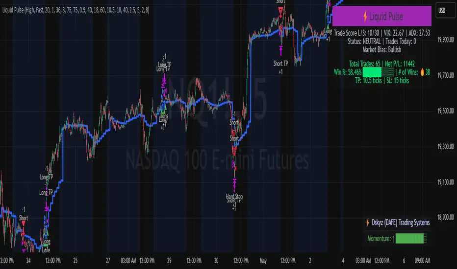
Liquid Pulse Liquid Pulse by Dskyz (DAFE) Trading Systems
Liquid Pulse is a trading algo built by Dskyz (DAFE) Trading Systems for futures markets like NQ1!, designed to snag high-probability trades with tight risk control. it fuses a confluence system—VWAP, MACD, ADX, volume, and liquidity sweeps—with a trade scoring setup, daily limits, and VIX pauses to dodge wild volatility. visuals include simple signals, VWAP bands, and a dashboard with stats.
Core Components for Liquid Pulse
Volume Sensitivity (volumeSensitivity) controls how much volume spikes matter for entries. options: 'Low', 'Medium', 'High' default: 'High' (catches small spikes, good for active markets) tweak it: 'Low' for calm markets, 'High' for chaos.
MACD Speed (macdSpeed) sets the MACD’s pace for momentum. options: 'Fast', 'Medium', 'Slow' default: 'Medium' (solid balance) tweak it: 'Fast' for scalping, 'Slow' for swings.
Daily Trade Limit (dailyTradeLimit) caps trades per day to keep risk in check. range: 1 to 30 default: 20 tweak it: 5-10 for safety, 20-30 for action.
Number of Contracts (numContracts) sets position size. range: 1 to 20 default: 4 tweak it: up for big accounts, down for small.
VIX Pause Level (vixPauseLevel) stops trading if VIX gets too hot. range: 10 to 80 default: 39.0 tweak it: 30 to avoid volatility, 50 to ride it.
Min Confluence Conditions (minConditions) sets how many signals must align. range: 1 to 5 default: 2 tweak it: 3-4 for strict, 1-2 for more trades.
Min Trade Score (Longs/Shorts) (minTradeScoreLongs/minTradeScoreShorts) filters trade quality. longs range: 0 to 100 default: 73 shorts range: 0 to 100 default: 75 tweak it: 80-90 for quality, 60-70 for volume.
Liquidity Sweep Strength (sweepStrength) gauges breakouts. range: 0.1 to 1.0 default: 0.5 tweak it: 0.7-1.0 for strong moves, 0.3-0.5 for small.
ADX Trend Threshold (adxTrendThreshold) confirms trends. range: 10 to 100 default: 41 tweak it: 40-50 for trends, 30-35 for weak ones.
ADX Chop Threshold (adxChopThreshold) avoids chop. range: 5 to 50 default: 20 tweak it: 15-20 to dodge chop, 25-30 to loosen.
VWAP Timeframe (vwapTimeframe) sets VWAP period. options: '15', '30', '60', '240', 'D' default: '60' (1-hour) tweak it: 60 for day, 240 for swing, D for long.
Take Profit Ticks (Longs/Shorts) (takeProfitTicksLongs/takeProfitTicksShorts) sets profit targets. longs range: 5 to 100 default: 25.0 shorts range: 5 to 100 default: 20.0 tweak it: 30-50 for trends, 10-20 for chop.
Max Profit Ticks (maxProfitTicks) caps max gain. range: 10 to 200 default: 60.0 tweak it: 80-100 for big moves, 40-60 for tight.
Min Profit Ticks to Trail (minProfitTicksTrail) triggers trailing. range: 1 to 50 default: 7.0 tweak it: 10-15 for big gains, 5-7 for quick locks.
Trailing Stop Ticks (trailTicks) sets trail distance. range: 1 to 50 default: 5.0 tweak it: 8-10 for room, 3-5 for fast locks.
Trailing Offset Ticks (trailOffsetTicks) sets trail offset. range: 1 to 20 default: 2.0 tweak it: 1-2 for tight, 5-10 for loose.
ATR Period (atrPeriod) measures volatility. range: 5 to 50 default: 9 tweak it: 14-20 for smooth, 5-9 for reactive.
Hardcoded Settings volLookback: 30 ('Low'), 20 ('Medium'), 11 ('High') volThreshold: 1.5 ('Low'), 1.8 ('Medium'), 2 ('High') swingLen: 5
Execution Logic Overview trades trigger when confluence conditions align, entering long or short with set position sizes. exits use dynamic take-profits, trailing stops after a profit threshold, hard stops via ATR, and a time stop after 100 bars.
Features Multi-Signal Confluence: needs VWAP, MACD, volume, sweeps, and ADX to line up.
Risk Control: ATR-based stops (capped 15 ticks), take-profits (scaled by volatility), and trails.
Market Filters: VIX pause, ADX trend/chop checks, volatility gates. Dashboard: shows scores, VIX, ADX, P/L, win %, streak.
Visuals Simple signals (green up triangles for longs, red down for shorts) and VWAP bands with glow. info table (bottom right) with MACD momentum. dashboard (top right) with stats.
Chart and Backtest:
NQ1! futures, 5-minute chart. works best in trending, volatile conditions. tweak inputs for other markets—test thoroughly.
Backtesting: NQ1! Frame: Jan 19, 2025, 09:00 — May 02, 2025, 16:00 Slippage: 3 Commission: $4.60
Fee Typical Range (per side, per contract)
CME Exchange $1.14 – $1.20
Clearing $0.10 – $0.30
NFA Regulatory $0.02
Firm/Broker Commis. $0.25 – $0.80 (retail prop)
TOTAL $1.60 – $2.30 per side
Round Turn: (enter+exit) = $3.20 – $4.60 per contract
Disclaimer this is for education only. past results don’t predict future wins. trading’s risky—only use money you can lose. backtest and validate before going live. (expect moderators to nitpick some random chart symbol rule—i’ll fix and repost if they pull it.)
About the Author Dskyz (DAFE) Trading Systems crafts killer trading algos. Liquid Pulse is pure research and grit, built for smart, bold trading. Use it with discipline. Use it with clarity. Trade smarter. I’ll keep dropping badass strategies ‘til i build a brand or someone signs me up.
2025 Created by Dskyz, powered by DAFE Trading Systems. Trade smart, trade bold.
ADR% Extension Levels from SMA 50I created this indicator inspired by RealSimpleAriel (a swing trader I recommend following on X) who does not buy stocks extended beyond 4 ADR% from the 50 SMA and uses extensions from the 50 SMA at 7-8-9-10-11-12-13 ADR% to take profits with a 20% position trimming.
RealSimpleAriel's strategy (as I understood it):
-> Focuses on leading stocks from leading groups and industries, i.e., those that have grown the most in the last 1-3-6 months (see on Finviz groups and then select sector-industry).
-> Targets stocks with the best technical setup for a breakout, above the 200 SMA in a bear market and above both the 50 SMA and 200 SMA in a bull market, selecting those with growing Earnings and Sales.
-> Buys stocks on breakout with a stop loss set at the day's low of the breakout and ensures they are not extended beyond 4 ADR% from the 50 SMA.
-> 3-5 day momentum burst: After a breakout, takes profits by selling 1/2 or 1/3 of the position after a 3-5 day upward move.
-> 20% trimming on extension from the 50 SMA: At 7 ADR% (ADR% calculated over 20 days) extension from the 50 SMA, takes profits by selling 20% of the remaining position. Continues to trim 20% of the remaining position based on the stock price extension from the 50 SMA, calculated using the 20-period ADR%, thus trimming 20% at 8-9-10-11 ADR% extension from the 50 SMA. Upon reaching 12-13 ADR% extension from the 50 SMA, considers the stock overextended, closes the remaining position, and evaluates a short.
-> Trailing stop with ascending SMA: Uses a chosen SMA (10, 20, or 50) as the definitive stop loss for the position, depending on the stock's movement speed (preferring larger SMAs for slower-moving stocks or for long-term theses). If the stock's closing price falls below the chosen SMA, the entire position is closed.
In summary:
-->Buy a breakout using the day's low of the breakout as the stop loss (this stop loss is the most critical).
--> Do not buy stocks extended beyond 4 ADR% from the 50 SMA.
--> Sell 1/2 or 1/3 of the position after 3-5 days of upward movement.
--> Trim 20% of the position at each 7-8-9-10-11-12-13 ADR% extension from the 50 SMA.
--> Close the entire position if the breakout fails and the day's low of the breakout is reached.
--> Close the entire position if the price, during the rise, falls below a chosen SMA (10, 20, or 50, depending on your preference).
--> Definitively close the position if it reaches 12-13 ADR% extension from the 50 SMA.
I used Grok from X to create this indicator. I am not a programmer, but based on the ADR% I use, it works.
Below is Grok from X's description of the indicator:
Script Description
The script is a custom indicator for TradingView that displays extension levels based on ADR% relative to the 50-period Simple Moving Average (SMA). Below is a detailed description of its features, structure, and behavior:
1. Purpose of the Indicator
Name: "ADR% Extension Levels from SMA 50".
Objective: Draw horizontal blue lines above and below the 50-period SMA, corresponding to specific ADR% multiples (4, 7, 8, 9, 10, 11, 12, 13). These levels represent potential price extension zones based on the average daily percentage volatility.
Overlay: The indicator is overlaid on the price chart (overlay=true), so the lines and SMA appear directly on the price graph.
2. Configurable Inputs
The indicator allows users to customize parameters through TradingView settings:
SMA Length (smaLength):
Default: 50 periods.
Description: Specifies the number of periods for calculating the Simple Moving Average (SMA). The 50-period SMA serves as the reference point for extension levels.
Constraint: Minimum 1 period.
ADR% Length (adrLength):
Default: 20 periods.
Description: Specifies the number of days to calculate the moving average of the daily high/low ratio, used to determine ADR%.
Constraint: Minimum 1 period.
Scale Factor (scaleFactor):
Default: 1.0.
Description: An optional multiplier to adjust the distance of extension levels from the SMA. Useful if levels are too close or too far due to an overly small or large ADR%.
Constraint: Minimum 0.1, increments of 0.1.
Tooltip: "Adjust if levels are too close or far from SMA".
3. Main Calculations
50-period SMA:
Calculated with ta.sma(close, smaLength) using the closing price (close).
Serves as the central line around which extension levels are drawn.
ADR% (Average Daily Range Percentage):
Formula: 100 * (ta.sma(dhigh / dlow, adrLength) - 1).
Details:
dhigh and dlow are the daily high and low prices, obtained via request.security(syminfo.tickerid, "D", high/low) to ensure data is daily-based, regardless of the chart's timeframe.
The dhigh / dlow ratio represents the daily percentage change.
The simple moving average (ta.sma) of this ratio over 20 days (adrLength) is subtracted by 1 and multiplied by 100 to obtain ADR% as a percentage.
The result is multiplied by scaleFactor for manual adjustments.
Extension Levels:
Defined as ADR% multiples: 4, 7, 8, 9, 10, 11, 12, 13.
Stored in an array (levels) for easy iteration.
For each level, prices above and below the SMA are calculated as:
Above: sma50 * (1 + (level * adrPercent / 100))
Below: sma50 * (1 - (level * adrPercent / 100))
These represent price levels corresponding to a percentage change from the SMA equal to level * ADR%.
4. Visualization
Horizontal Blue Lines:
For each level (4, 7, 8, 9, 10, 11, 12, 13 ADR%), two lines are drawn:
One above the SMA (e.g., +4 ADR%).
One below the SMA (e.g., -4 ADR%).
Color: Blue (color.blue).
Style: Solid (style=line.style_solid).
Management:
Each level has dedicated variables for upper and lower lines (e.g., upperLine1, lowerLine1 for 4 ADR%).
Previous lines are deleted with line.delete before drawing new ones to avoid overlaps.
Lines are updated at each bar with line.new(bar_index , level, bar_index, level), covering the range from the previous bar to the current one.
Labels:
Displayed only on the last bar (barstate.islast) to avoid clutter.
For each level, two labels:
Above: E.g., "4 ADR%", positioned above the upper line (style=label.style_label_down).
Below: E.g., "-4 ADR%", positioned below the lower line (style=label.style_label_up).
Color: Blue background, white text.
50-period SMA:
Drawn as a gray line (color.gray) for visual reference.
Diagnostics:
ADR% Plot: ADR% is plotted in the status line (orange, histogram style) to verify the value.
ADR% Label: A label on the last bar near the SMA shows the exact ADR% value (e.g., "ADR%: 2.34%"), with a gray background and white text.
5. Behavior
Dynamic Updating:
Lines update with each new bar to reflect new SMA 50 and ADR% values.
Since ADR% uses daily data ("D"), it remains constant within the same day but changes day-to-day.
Visibility Across All Bars:
Lines are drawn on every bar, not just the last one, ensuring visibility on historical data as well.
Adaptability:
The scaleFactor allows level adjustments if ADR% is too small (e.g., for low-volatility symbols) or too large (e.g., for cryptocurrencies).
Compatibility:
Works on any timeframe since ADR% is calculated from daily data.
Suitable for symbols with varying volatility (e.g., stocks, forex, cryptocurrencies).
6. Intended Use
Technical Analysis: Extension levels represent significant price zones based on average daily volatility. They can be used to:
Identify potential price targets (e.g., take profit at +7 ADR%).
Assess support/resistance zones (e.g., -4 ADR% as support).
Measure price extension relative to the 50 SMA.
Trading: Useful for strategies based on breakouts or mean reversion, where ADR% levels indicate reversal or continuation points.
Debugging: Labels and ADR% plot help verify that values align with the symbol’s volatility.
7. Limitations
Dependence on Daily Data: ADR% is based on daily dhigh/dlow, so it may not reflect intraday volatility on short timeframes (e.g., 1 minute).
Extreme ADR% Values: For low-volatility symbols (e.g., bonds) or high-volatility symbols (e.g., meme stocks), ADR% may require adjustments via scaleFactor.
Graphical Load: Drawing 16 lines (8 upper, 8 lower) on every bar may slow the chart for very long historical periods, though line management is optimized.
ADR% Formula: The formula 100 * (sma(dhigh/dlow, Length) - 1) may produce different values compared to other ADR% definitions (e.g., (high - low) / close * 100), so users should be aware of the context.
8. Visual Example
On a chart of a stock like TSLA (daily timeframe):
The 50 SMA is a gray line tracking the average trend.
Assuming an ADR% of 3%:
At +4 ADR% (12%), a blue line appears at sma50 * 1.12.
At -4 ADR% (-12%), a blue line appears at sma50 * 0.88.
Other lines appear at ±7, ±8, ±9, ±10, ±11, ±12, ±13 ADR%.
On the last bar, labels show "4 ADR%", "-4 ADR%", etc., and a gray label shows "ADR%: 3.00%".
ADR% is visible in the status line as an orange histogram.
9. Code: Technical Structure
Language: Pine Script @version=5.
Inputs: Three configurable parameters (smaLength, adrLength, scaleFactor).
Calculations:
SMA: ta.sma(close, smaLength).
ADR%: 100 * (ta.sma(dhigh / dlow, adrLength) - 1) * scaleFactor.
Levels: sma50 * (1 ± (level * adrPercent / 100)).
Graphics:
Lines: Created with line.new, deleted with line.delete to avoid overlaps.
Labels: Created with label.new only on the last bar.
Plots: plot(sma50) for the SMA, plot(adrPercent) for debugging.
Optimization: Uses dedicated variables for each line (e.g., upperLine1, lowerLine1) for clear management and to respect TradingView’s graphical object limits.
10. Possible Improvements
Option to show lines only on the last bar: Would reduce visual clutter.
Customizable line styles: Allow users to choose color or style (e.g., dashed).
Alert for anomalous ADR%: A message if ADR% is too small or large.
Dynamic levels: Allow users to specify ADR% multiples via input.
Optimization for short timeframes: Adapt ADR% for intraday timeframes.
Conclusion
The script creates a visual indicator that helps traders identify price extension levels based on daily volatility (ADR%) relative to the 50 SMA. It is robust, configurable, and includes debugging tools (ADR% plot and labels) to verify values. The ADR% formula based on dhigh/dlow

Green*DiamondGreen*Diamond (GD1)
Unleash Dynamic Trading Signals with Volatility and Momentum
Overview
GreenDiamond is a versatile overlay indicator designed for traders seeking actionable buy and sell signals across various markets and timeframes. Combining Volatility Bands (VB) bands, Consolidation Detection, MACD, RSI, and a unique Ribbon Wave, it highlights high-probability setups while filtering out noise. With customizable signals like Green-Yellow Buy, Pullback Sell, and Inverse Pullback Buy, plus vibrant candle and volume visuals, GreenDiamond adapts to your trading style—whether you’re scalping, day trading, or swing trading.
Key Features
Volatility Bands (VB): Plots dynamic upper and lower bands to identify breakouts or reversals, with toggleable buy/sell signals outside consolidation zones.
Consolidation Detection: Marks low-range periods to avoid choppy markets, ensuring signals fire during trending conditions.
MACD Signals: Offers flexible buy/sell conditions (e.g., cross above signal, above zero, histogram up) with RSI divergence integration for precision.
RSI Filter: Enhances signals with customizable levels (midline, oversold/overbought) and bullish divergence detection.
Ribbon Wave: Visualizes trend strength using three EMAs, colored by MACD and RSI for intuitive momentum cues.
Custom Signals: Includes Green-Yellow Buy, Pullback Sell, and Inverse Pullback Buy, with limits on consecutive signals to prevent overtrading.
Candle & Volume Styling: Blends MACD/RSI colors on candles and scales volume bars to highlight momentum spikes.
Alerts: Set up alerts for VB signals, MACD crosses, Green*Diamond signals, and custom conditions to stay on top of opportunities.
How It Works
Green*Diamond integrates multiple indicators to generate signals:
Volatility Bands: Calculates bands using a pivot SMA and standard deviation. Buy signals trigger on crossovers above the lower band, sell signals on crossunders below the upper band (if enabled).
Consolidation Filter: Suppresses signals when candle ranges are below a threshold, keeping you out of flat markets.
MACD & RSI: Combines MACD conditions (e.g., cross above signal) with RSI filters (e.g., above midline) and optional volume spikes for robust signals.
Custom Logic: Green-Yellow Buy uses MACD bullishness, Pullback Sell targets retracements, and Inverse Pullback Buy catches reversals after downmoves—all filtered to avoid consolidation.
Visuals: Ribbon Wave shows trend direction, candles blend momentum colors, and volume bars scale dynamically to confirm signals.
Settings
Volatility Bands Settings:
VB Lookback Period (20): Adjust to 10–15 for faster markets (e.g., 1-minute scalping) or 25–30 for daily charts.
Upper/Lower Band Multiplier (1.0): Increase to 1.5–2.0 for wider bands in volatile stocks like AEHL; decrease to 0.5 for calmer markets.
Show Volatility Bands: Toggle off to reduce chart clutter.
Use VB Signals: Enable for breakout-focused trades; disable to focus on Green*Diamond signals.
Consolidation Settings:
Consolidation Lookback (14): Set to 5–10 for small caps (e.g., AEHL) to catch quick consolidations; 20 for higher timeframes.
Range Threshold (0.5): Lower to 0.3 for stricter filtering in choppy markets; raise to 0.7 for looser signals.
MACD Settings:
Fast/Slow Length (12/26): Shorten to 8/21 for scalping; extend to 15/34 for swing trading.
Signal Smoothing (9): Reduce to 5 for faster signals; increase to 12 for smoother trends.
Buy/Sell Signal Options: Choose “Cross Above Signal” for classic MACD; “Histogram Up” for momentum plays.
Use RSI Div + MACD Cross: Enable for high-probability reversal signals.
RSI Settings:
RSI Period (14): Drop to 10 for 1-minute charts; raise to 20 for daily.
Filter Level (50): Set to 55 for stricter buys; 45 for sells.
Overbought/Oversold (70/30): Tighten to 65/35 for small caps; widen to 75/25 for indices.
RSI Buy/Sell Options: Select “Bullish Divergence” for reversals; “Cross Above Oversold” for momentum.
Color Settings:
Adjust bullish/bearish colors for visibility (e.g., brighter green/red for dark themes).
Border Thickness (1): Increase to 2–3 for clearer candle outlines.
Volume Settings:
Volume Average Length (20): Shorten to 10 for scalping; extend to 30 for swing trades.
Volume Multiplier (2.0): Raise to 3.0 for AEHL’s volume surges; lower to 1.5 for steady stocks.
Bar Height (10%): Increase to 15% for prominent bars; decrease to 5% to reduce clutter.
Ribbon Settings:
EMA Periods (10/20/30): Tighten to 5/10/15 for scalping; widen to 20/40/60 for trends.
Color by MACD/RSI: Disable for simpler visuals; enable for dynamic momentum cues.
Gradient Fill: Toggle on for trend clarity; off for minimalism.
Custom Signals:
Enable Green-Yellow Buy: Use for momentum confirmation; limit to 1–2 signals to avoid spam.
Pullback/Inverse Pullback % (50): Set to 30–40% for small caps; 60–70% for indices.
Max Buy Signals (1): Increase to 2–3 for active markets; keep at 1 for discipline.
Tips and Tricks
Scalping Small Caps (e.g., AEHL):
Use 1-minute charts with VB Lookback = 10, Consolidation Lookback = 5, and Volume Multiplier = 3.0 to catch $0.10–$0.20 moves.
Enable Green-Yellow Buy and Inverse Pullback Buy for quick entries; disable VB Signals to focus on Green*Diamond logic.
Pair with SMC+ green boxes (if you use them) for reversal confirmation.
Day Trading:
Try 5-minute charts with MACD Fast/Slow = 8/21 and RSI Period = 10.
Enable RSI Divergence + MACD Cross for high-probability setups; set Max Buy Signals = 2.
Watch for volume bars turning yellow to confirm entries.
Swing Trading:
Use daily charts with VB Lookback = 30, Ribbon EMAs = 20/40/60.
Enable Pullback Sell (60%) to exit after rallies; disable RSI Color for cleaner candles.
Check Ribbon Wave gradient for trend strength—bright green signals strong bulls.
Avoiding Noise:
Increase Consolidation Threshold to 0.7 on volatile days to skip false breakouts.
Disable Ribbon Wave or Volume Bars if the chart feels crowded.
Limit Max Buy Signals to 1 for disciplined trading.
Alert Setup:
In TradingView’s Alerts panel, select:
“GD Buy Signal” for standard entries.
“RSI Div + MACD Cross Buy” for reversals.
“VB Buy Signal” for breakout plays.
Set to “Once Per Bar Close” for confirmed signals; “Once Per Bar” for scalping.
Backtesting:
Replay on small caps ( Float < 5M, Price $0.50–$5) to test signals.
Focus on “GD Buy Signal” with yellow volume bars and green Ribbon Wave.
Avoid signals during gray consolidation squares unless paired with RSI Divergence.
Usage Notes
Markets: Works on stocks, forex, crypto, and indices. Best for volatile assets (e.g., small-cap stocks, BTCUSD).
Timeframes: Scalping (1–5 minutes), day trading (15–60 minutes), or swing trading (daily). Adjust settings per timeframe.
Risk Management: Combine with stop-losses (e.g., 1% risk, $0.05 below AEHL entry) and take-profits (3–5%).
Customization: Tweak inputs to match your strategy—experiment in replay to find your sweet spot.
Disclaimer
Green*Diamond is a technical tool to assist with trade identification, not a guarantee of profits. Trading involves risks, and past performance doesn’t predict future results. Always conduct your own analysis, manage risk, and test settings before live trading.
Feedback
Love Green*Diamond? Found a killer setup?

Accurate Bollinger Bands mcbw_ [True Volatility Distribution]The Bollinger Bands have become a very important technical tool for discretionary and algorithmic traders alike over the last decades. It was designed to give traders an edge on the markets by setting probabilistic values to different levels of volatility. However, some of the assumptions that go into its calculations make it unusable for traders who want to get a correct understanding of the volatility that the bands are trying to be used for. Let's go through what the Bollinger Bands are said to show, how their calculations work, the problems in the calculations, and how the current indicator I am presenting today fixes these.
--> If you just want to know how the settings work then skip straight to the end or click on the little (i) symbol next to the values in the indicator settings window when its on your chart <--
--------------------------- What Are Bollinger Bands ---------------------------
The Bollinger Bands were formed in the 1980's, a time when many retail traders interacted with their symbols via physically printed charts and computer memory for personal computer memory was measured in Kb (about a factor of 1 million smaller than today). Bollinger Bands are designed to help a trader or algorithm see the likelihood of price expanding outside of its typical range, the further the lines are from the current price implies the less often they will get hit. With a hands on understanding many strategies use these levels for designated levels of breakout trades or to assist in defining price ranges.
--------------------------- How Bollinger Bands Work ---------------------------
The calculations that go into Bollinger Bands are rather simple. There is a moving average that centers the indicator and an equidistant top band and bottom band are drawn at a fixed width away. The moving average is just a typical moving average (or common variant) that tracks the price action, while the distance to the top and bottom bands is a direct function of recent price volatility. The way that the distance to the bands is calculated is inspired by formulas from statistics. The standard deviation is taken from the candles that go into the moving average and then this is multiplied by a user defined value to set the bands position, I will call this value 'the multiple'. When discussing Bollinger Bands, that trading community at large normally discusses 'the multiple' as a multiplier of the standard deviation as it applies to a normal distribution (gaußian probability). On a normal distribution the number of standard deviations away (which trades directly use as 'the multiple') you are directly corresponds to how likely/unlikely something is to happen:
1 standard deviation equals 68.3%, meaning that the price should stay inside the 1 standard deviation 68.3% of the time and be outside of it 31.7% of the time;
2 standard deviation equals 95.5%, meaning that the price should stay inside the 2 standard deviation 95.5% of the time and be outside of it 4.5% of the time;
3 standard deviation equals 99.7%, meaning that the price should stay inside the 3 standard deviation 99.7% of the time and be outside of it 0.3% of the time.
Therefore when traders set 'the multiple' to 2, they interpret this as meaning that price will not reach there 95.5% of the time.
---------------- The Problem With The Math of Bollinger Bands ----------------
In and of themselves the Bollinger Bands are a great tool, but they have become misconstrued with some incorrect sense of statistical meaning, when they should really just be taken at face value without any further interpretation or implication.
In order to explain this it is going to get a bit technical so I will give a little math background and try to simplify things. First let's review some statistics topics (distributions, percentiles, standard deviations) and then with that understanding explore the incorrect logic of how Bollinger Bands have been interpreted/employed.
---------------- Quick Stats Review ----------------
.
(If you are comfortable with statistics feel free to skip ahead to the next section)
.
-------- I: Probability distributions --------
When you have a lot of data it is helpful to see how many times different results appear in your dataset. To visualize this people use "histograms", which just shows how many times each element appears in the dataset by stacking each of the same elements on top of each other to form a graph. You may be familiar with the bell curve (also called the "normal distribution", which we will be calling it by). The normal distribution histogram looks like a big hump around zero and then drops off super quickly the further you get from it. This shape (the bell curve) is very nice because it has a lot of very nifty mathematical properties and seems to show up in nature all the time. Since it pops up in so many places, society has developed many different shortcuts related to it that speed up all kinds of calculations, including the shortcut that 1 standard deviation = 68.3%, 2 standard deviations = 95.5%, and 3 standard deviations = 99.7% (these only apply to the normal distribution). Despite how handy the normal distribution is and all the shortcuts we have for it are, and how much it shows up in the natural world, there is nothing that forces your specific dataset to look like it. In fact, your data can actually have any possible shape. As we will explore later, economic and financial datasets *rarely* follow the normal distribution.
-------- II: Percentiles --------
After you have made the histogram of your dataset you have built the "probability distribution" of your own dataset that is specific to all the data you have collected. There is a whole complicated framework for how to accurately calculate percentiles but we will dramatically simplify it for our use. The 'percentile' in our case is just the number of data points we are away from the "middle" of the data set (normally just 0). Lets say I took the difference of the daily close of a symbol for the last two weeks, green candles would be positive and red would be negative. In this example my dataset of day by day closing price difference is:
week 1:
week 2:
sorting all of these value into a single dataset I have:
I can separate the positive and negative returns and explore their distributions separately:
negative return distribution =
positive return distribution =
Taking the 25th% percentile of these would just be taking the value that is 25% towards the end of the end of these returns. Or akin the 100%th percentile would just be taking the vale that is 100% at the end of those:
negative return distribution (50%) = -5
positive return distribution (50%) = +4
negative return distribution (100%) = -10
positive return distribution (100%) = +20
Or instead of separating the positive and negative returns we can also look at all of the differences in the daily close as just pure price movement and not account for the direction, in this case we would pool all of the data together by ignoring the negative signs of the negative reruns
combined return distribution =
In this case the 50%th and 100%th percentile of the combined return distribution would be:
combined return distribution (50%) = 4
combined return distribution (100%) = 10
Sometimes taking the positive and negative distributions separately is better than pooling them into a combined distribution for some purposes. Other times the combined distribution is better.
Most financial data has very different distributions for negative returns and positive returns. This is encapsulated in sayings like "Price takes the stairs up and the elevator down".
-------- III: Standard Deviation --------
The formula for the standard deviation (refereed to here by its shorthand 'STDEV') can be intimidating, but going through each of its elements will illuminate what it does. The formula for STDEV is equal to:
square root ( (sum ) / N )
Going back the the dataset that you might have, the variables in the formula above are:
'mean' is the average of your entire dataset
'x' is just representative of a single point in your dataset (one point at a time)
'N' is the total number of things in your dataset.
Going back to the STDEV formula above we can see how each part of it works. Starting with the '(x - mean)' part. What this does is it takes every single point of the dataset and measure how far away it is from the mean of the entire dataset. Taking this value to the power of two: '(x - mean) ^ 2', means that points that are very far away from the dataset mean get 'penalized' twice as much. Points that are very close to the dataset mean are not impacted as much. In practice, this would mean that if your dataset had a bunch of values that were in a wide range but always stayed in that range, this value ('(x - mean) ^ 2') would end up being small. On the other hand, if your dataset was full of the exact same number, but had a couple outliers very far away, this would have a much larger value since the square par of '(x - mean) ^ 2' make them grow massive. Now including the sum part of 'sum ', this just adds up all the of the squared distanced from the dataset mean. Then this is divided by the number of values in the dataset ('N'), and then the square root of that value is taken.
There is nothing inherently special or definitive about the STDEV formula, it is just a tool with extremely widespread use and adoption. As we saw here, all the STDEV formula is really doing is measuring the intensity of the outliers.
--------------------------- Flaws of Bollinger Bands ---------------------------
The largest problem with Bollinger Bands is the assumption that price has a normal distribution. This is assumption is massively incorrect for many reasons that I will try to encapsulate into two points:
Price return do not follow a normal distribution, every single symbol on every single timeframe has is own unique distribution that is specific to only itself. Therefore all the tools, shortcuts, and ideas that we use for normal distributions do not apply to price returns, and since they do not apply here they should not be used. A more general approach is needed that allows each specific symbol on every specific timeframe to be treated uniquely.
The distributions of price returns on the positive and negative side are almost never the same. A more general approach is needed that allows positive and negative returns to be calculated separately.
In addition to the issues of the normal distribution assumption, the standard deviation formula (as shown above in the quick stats review) is essentially just a tame measurement of outliers (a more aggressive form of outlier measurement might be taking the differences to the power of 3 rather than 2). Despite this being a bit of a philosophical question, does the measurement of outlier intensity as defined by the STDEV formula really measure what we want to know as traders when we're experiencing volatility? Or would adjustments to that formula better reflect what we *experience* as volatility when we are actively trading? This is an open ended question that I will leave here, but I wanted to pose this question because it is a key part of what how the Bollinger Bands work that we all assume as a given.
Circling back on the normal distribution assumption, the standard deviation formula used in the calculation of the bands only encompasses the deviation of the candles that go into the moving average and have no knowledge of the historical price action. Therefore the level of the bands may not really reflect how the price action behaves over a longer period of time.
------------ Delivering Factually Accurate Data That Traders Need------------
In light of the problems identified above, this indicator fixes all of these issue and delivers statistically correct information that discretionary and algorithmic traders can use, with truly accurate probabilities. It takes the price action of the last 2,000 candles and builds a huge dataset of distributions that you can directly select your percentiles from. It also allows you to have the positive and negative distributions calculated separately, or if you would like, you can pool all of them together in a combined distribution. In addition to this, there is a wide selection of moving averages directly available in the indicator to choose from.
Hedge funds, quant shops, algo prop firms, and advanced mechanical groups all employ the true return distributions in their work. Now you have access to the same type of data with this indicator, wherein it's doing all the lifting for you.
------------------------------ Indicator Settings ------------------------------
.
---- Moving average ----
Select the type of moving average you would like and its length
---- Bands ----
The percentiles that you enter here will be pulled directly from the return distribution of the last 2,000 candles. With the typical Bollinger Bands, traders would select 2 standard deviations and incorrectly think that the levels it highlights are the 95.5% levels. Now, if you want the true 95.5% level, you can just enter 95.5 into the percentile value here. Each of the three available bands takes the true percentile you enter here.
---- Separate Positive & Negative Distributions----
If this box is checked the positive and negative distributions are treated indecently, completely separate from each other. You will see that the width of the top and bottom bands will be different for each of the percentiles you enter.
If this box is unchecked then all the negative and positive distributions are pooled together. You will notice that the width of the top and bottom bands will be the exact same.
---- Distribution Size ----
This is the number of candles that the price return is calculated over. EG: to collect the price return over the last 33 candles, the difference of price from now to 33 candles ago is calculated for the last 2,000 candles, to build a return distribution of 2000 points of price differences over 33 candles.
NEGATIVE NUMBERS(<0) == exact number of candles to include;
EG: setting this value to -20 will always collect volatility distributions of 20 candles
POSITIVE NUMBERS(>0) == number of candles to include as a multiple of the Moving Average Length value set above;
EG: if the Moving Average Length value is set to 22, setting this value to 2 will use the last 22*2 = 44 candles for the collection of volatility distributions
MORE candles being include will generally make the bands WIDER and their size will change SLOWER over time.
I wish you focus, dedication, and earnest success on your journey.
Happy trading :)

Quantum Market Analyzer X7Quantum Market Analyzer X7 - Complete Study Guide
Table of Contents
1. Overview
2. Indicator Components
3. Signal Interpretation
4. Live Market Analysis Guide
5. Best Practices
6. Limitations and Considerations
7. Risk Disclaimer
________________________________________
Overview
The Quantum Market Analyzer X7 is a comprehensive multi-timeframe technical analysis indicator that combines traditional and modern analytical methods. It aggregates signals from multiple technical indicators across seven key analysis categories to provide traders with a consolidated view of market sentiment and potential trading opportunities.
Key Features:
• Multi-Indicator Analysis: Combines 20+ technical indicators
• Real-Time Dashboard: Professional interface with customizable display
• Signal Aggregation: Weighted scoring system for overall market sentiment
• Advanced Analytics: Includes Order Block detection, Supertrend, and Volume analysis
• Visual Progress Indicators: Easy-to-read progress bars for signal strength
________________________________________
Indicator Components
1. Oscillators Section
Purpose: Identifies overbought/oversold conditions and momentum changes
Included Indicators:
• RSI (14): Relative Strength Index - momentum oscillator
• Stochastic (14): Compares closing price to price range
• CCI (20): Commodity Channel Index - cycle identification
• Williams %R (14): Momentum indicator similar to Stochastic
• MACD (12,26,9): Moving Average Convergence Divergence
• Momentum (10): Rate of price change
• ROC (9): Rate of Change
• Bollinger Bands (20,2): Volatility-based indicator
Signal Interpretation:
• Strong Buy (6+ points): Multiple oscillators indicate oversold conditions
• Buy (2-5 points): Moderate bullish momentum
• Neutral (-1 to 1 points): Balanced conditions
• Sell (-2 to -5 points): Moderate bearish momentum
• Strong Sell (-6+ points): Multiple oscillators indicate overbought conditions
2. Moving Averages Section
Purpose: Determines trend direction and strength
Included Indicators:
• SMA: 10, 20, 50, 100, 200 periods
• EMA: 10, 20, 50 periods
Signal Logic:
• Price >2% above MA = Strong Buy (+2)
• Price above MA = Buy (+1)
• Price below MA = Sell (-1)
• Price >2% below MA = Strong Sell (-2)
Signal Interpretation:
• Strong Buy (6+ points): Price well above multiple MAs, strong uptrend
• Buy (2-5 points): Price above most MAs, bullish trend
• Neutral (-1 to 1 points): Mixed MA signals, consolidation
• Sell (-2 to -5 points): Price below most MAs, bearish trend
• Strong Sell (-6+ points): Price well below multiple MAs, strong downtrend
3. Order Block Analysis
Purpose: Identifies institutional support/resistance levels and breakouts
How It Works:
• Detects historical levels where large orders were placed
• Monitors price behavior around these levels
• Identifies breakouts from established order blocks
Signal Types:
• BULLISH BRK (+2): Breakout above resistance order block
• BEARISH BRK (-2): Breakdown below support order block
• ABOVE SUP (+1): Price holding above support
• BELOW RES (-1): Price rejected at resistance
• NEUTRAL (0): No significant order block interaction
4. Supertrend Analysis
Purpose: Trend following indicator based on Average True Range
Parameters:
• ATR Period: 10 (default)
• ATR Multiplier: 6.0 (default)
Signal Types:
• BULLISH (+2): Price above Supertrend line
• BEARISH (-2): Price below Supertrend line
• NEUTRAL (0): Transition period
5. Trendline/Channel Analysis
Purpose: Identifies trend channels and breakout patterns
Components:
• Dynamic trendline calculation using pivot points
• Channel width based on historical volatility
• Breakout detection algorithm
Signal Types:
• UPPER BRK (+2): Breakout above upper channel
• LOWER BRK (-2): Breakdown below lower channel
• ABOVE MID (+1): Price above channel midline
• BELOW MID (-1): Price below channel midline
6. Volume Analysis
Purpose: Confirms price movements with volume data
Components:
• Volume spikes detection
• On Balance Volume (OBV)
• Volume Price Trend (VPT)
• Money Flow Index (MFI)
• Accumulation/Distribution Line
Signal Calculation: Multiple volume indicators are combined to determine institutional activity and confirm price movements.
________________________________________
Signal Interpretation
Overall Summary Signals
The indicator aggregates all component signals into an overall market sentiment:
Signal Score Range Interpretation Action
STRONG BUY 10+ Overwhelming bullish consensus Consider long positions
BUY 4-9 Moderate to strong bullish bias Look for long opportunities
NEUTRAL -3 to 3 Mixed signals, consolidation Wait for clearer direction
SELL -4 to -9 Moderate to strong bearish bias Look for short opportunities
STRONG SELL -10+ Overwhelming bearish consensus Consider short positions
Progress Bar Interpretation
• Filled bars indicate signal strength
• Green bars: Bullish signals
• Red bars: Bearish signals
• More filled bars = stronger conviction
________________________________________
Live Market Analysis Guide
Step 1: Initial Assessment
1. Check Overall Summary: Start with the main signal
2. Verify with Component Analysis: Ensure signals align
3. Look for Divergences: Identify conflicting signals
Step 2: Timeframe Analysis
1. Set Appropriate Timeframe: Use 1H for intraday, 4H/1D for swing trading
2. Multi-Timeframe Confirmation: Check higher timeframes for trend context
3. Entry Timing: Use lower timeframes for precise entry points
Step 3: Signal Confirmation Process
For Buy Signals:
1. Oscillators: Look for oversold conditions (RSI <30, Stoch <20)
2. Moving Averages: Price should be above key MAs
3. Order Blocks: Confirm bounce from support levels
4. Volume: Check for accumulation patterns
5. Supertrend: Ensure bullish trend alignment
For Sell Signals:
1. Oscillators: Look for overbought conditions (RSI >70, Stoch >80)
2. Moving Averages: Price should be below key MAs
3. Order Blocks: Confirm rejection at resistance levels
4. Volume: Check for distribution patterns
5. Supertrend: Ensure bearish trend alignment
Step 4: Risk Management Integration
1. Signal Strength Assessment: Stronger signals = larger position size
2. Stop Loss Placement: Use Order Block levels for stops
3. Take Profit Targets: Based on channel analysis and resistance levels
4. Position Sizing: Adjust based on signal confidence
________________________________________
Best Practices
Entry Strategies
1. High Conviction Entries: Wait for STRONG BUY/SELL signals
2. Confluence Trading: Look for multiple components aligning
3. Breakout Trading: Use Order Block and Trendline breakouts
4. Trend Following: Align with Supertrend direction
Risk Management
1. Never Risk More Than 2% Per Trade: Regardless of signal strength
2. Use Stop Losses: Place at invalidation levels
3. Scale Positions: Stronger signals warrant larger (but still controlled) positions
4. Diversification: Don't rely solely on one indicator
Market Conditions
1. Trending Markets: Focus on Supertrend and MA signals
2. Range-Bound Markets: Emphasize Oscillator and Order Block signals
3. High Volatility: Reduce position sizes, widen stops
4. Low Volume: Be cautious of breakout signals
Common Mistakes to Avoid
1. Signal Chasing: Don't enter after signals have already moved significantly
2. Ignoring Context: Consider overall market conditions
3. Overtrading: Wait for high-quality setups
4. Poor Risk Management: Always use appropriate position sizing
________________________________________
Limitations and Considerations
Technical Limitations
1. Lagging Nature: All technical indicators are based on historical data
2. False Signals: No indicator is 100% accurate
3. Market Regime Changes: Indicators may perform differently in various market conditions
4. Whipsaws: Possible in choppy, sideways markets
Optimal Use Cases
1. Trending Markets: Performs best in clear trending environments
2. Medium to High Volatility: Requires sufficient price movement for signals
3. Liquid Markets: Works best with adequate volume and tight spreads
4. Multiple Timeframe Analysis: Most effective when used across different timeframes
When to Use Caution
1. Major News Events: Fundamental analysis may override technical signals
2. Market Opens/Closes: Higher volatility can create false signals
3. Low Volume Periods: Signals may be less reliable
4. Holiday Trading: Reduced participation affects signal quality
________________________________________
Risk Disclaimer
IMPORTANT LEGAL DISCLAIMER FROM aiTrendview
WARNING: TRADING INVOLVES SUBSTANTIAL RISK OF LOSS
This Quantum Market Analyzer X7 indicator ("the Indicator") is provided for educational and informational purposes only. By using this indicator, you acknowledge and agree to the following terms:
No Investment Advice
• The Indicator does NOT constitute investment advice, financial advice, or trading recommendations
• All signals generated are based on historical price data and mathematical calculations
• Past performance does not guarantee future results
• No representation is made that any account will achieve profits or losses similar to those shown
Risk Acknowledgment
• TRADING CARRIES SUBSTANTIAL RISK: You may lose some or all of your invested capital
• LEVERAGE AMPLIFIES RISK: Margin trading can result in losses exceeding your initial investment
• MARKET VOLATILITY: Financial markets are inherently unpredictable and volatile
• TECHNICAL ANALYSIS LIMITATIONS: No technical indicator is infallible or guarantees profitable trades
User Responsibility
• YOU ARE SOLELY RESPONSIBLE for all trading decisions and their consequences
• CONDUCT YOUR OWN RESEARCH: Always perform independent analysis before making trading decisions
• CONSULT PROFESSIONALS: Seek advice from qualified financial advisors
• RISK MANAGEMENT: Implement appropriate risk management strategies
No Warranties
• The Indicator is provided "AS IS" without warranties of any kind
• aiTrendview makes no representations about the accuracy, reliability, or suitability of the Indicator
• Technical glitches, data feed issues, or calculation errors may occur
• The Indicator may not work as expected in all market conditions
Limitation of Liability
• aiTrendview SHALL NOT BE LIABLE for any direct, indirect, incidental, or consequential damages
• This includes but is not limited to: trading losses, missed opportunities, data inaccuracies, or system failures
• MAXIMUM LIABILITY is limited to the amount paid for the indicator (if any)
Code Usage and Distribution
• This indicator is published on TradingView in accordance with TradingView's house rules
• UNAUTHORIZED MODIFICATION or redistribution of this code is prohibited
• Users may not claim ownership of this intellectual property
• Commercial use requires explicit written permission from aiTrendview
Compliance and Regulations
• VERIFY LOCAL REGULATIONS: Ensure compliance with your jurisdiction's trading laws
• Some trading strategies may not be suitable for all investors
• Tax implications of trading are your responsibility
• Report trading activities as required by law
Specific Risk Factors
1. False Signals: The Indicator may generate incorrect buy/sell signals
2. Market Gaps: Overnight gaps can invalidate technical analysis
3. Fundamental Events: News and economic data can override technical signals
4. Liquidity Risk: Some markets may have insufficient liquidity
5. Technology Risk: Platform failures or connectivity issues may prevent order execution
Professional Trading Warning
• THIS IS NOT PROFESSIONAL TRADING SOFTWARE: Not intended for institutional or professional trading
• NO REGULATORY APPROVAL: This indicator has not been approved by any financial regulatory authority
• EDUCATIONAL PURPOSE: Designed primarily for learning technical analysis concepts
FINAL WARNING
NEVER INVEST MONEY YOU CANNOT AFFORD TO LOSE
Trading financial instruments involves significant risk. The majority of retail traders lose money. Before using this indicator in live trading:
1. Practice on paper/demo accounts extensively
2. Start with small position sizes
3. Develop a comprehensive trading plan
4. Implement strict risk management rules
5. Continuously educate yourself about market dynamics
By using the Quantum Market Analyzer X7, you acknowledge that you have read, understood, and agree to this disclaimer. You assume full responsibility for all trading decisions and their outcomes.
Contact: For questions about this disclaimer or the indicator, contact aiTrendview through official TradingView channels only.
________________________________________
This study guide and indicator are published on TradingView in compliance with TradingView's community guidelines and house rules. All users must adhere to TradingView's terms of service when using this indicator.
Document Version: 1.0
Last Updated: September 2025
Publisher: aiTrendview
________________________________________
Disclaimer from aiTrendview.com
The content provided in this blog post is for educational and training purposes only. It is not intended to be, and should not be construed as, financial, investment, or trading advice. All charting and technical analysis examples are for illustrative purposes. Trading and investing in financial markets involve substantial risk of loss and are not suitable for every individual. Before making any financial decisions, you should consult with a qualified financial professional to assess your personal financial situation.

Multi-Timeframe EMA Alignment + Listing InfoEnhanced EMA Alignment Checks
Original 4-EMA rows: Check 10EMA ≥ 20EMA ≥ 50EMA ≥ 200EMA for all timeframes
New 3-EMA rows: Check 10EMA ≥ 20EMA ≥ 50EMA (without 200EMA requirement) for weekly and monthly timeframes
Visual Distinction
White background: 4-EMA alignment rows (standard check)
Yellow background: 3-EMA alignment rows (less restrictive check)
Asterisk notation: "1W*" and "1M*" indicate the 3-EMA version
Complete Table Layout
1H: 4-EMA alignment (10≥20≥50≥200)
1D: 4-EMA alignment (10≥20≥50≥200)
1W: 4-EMA alignment (10≥20≥50≥200)
1M: 4-EMA alignment (10≥20≥50≥200)
1W* : 3-EMA alignment (10≥20≥50) - NEW
1M* : 3-EMA alignment (10≥20≥50) - NEW
Separator line
Since List: Weeks/months since listing
Benefits of This Setup:
Comprehensive Analysis: You can now see both strict (4-EMA) and relaxed (3-EMA) trend conditions
Better Entry Signals: The 3-EMA alignment might trigger earlier than 4-EMA, providing potential early entry signals
Trend Strength Assessment: When both 3-EMA and 4-EMA are aligned, it indicates very strong trend conditions
Flexible Strategy: You can use 3-EMA for trend following and 4-EMA for confirmation
The table now provides a complete multi-timeframe trend analysis with both conservative and aggressive alignment criteria, giving you more flexibility in your trading decisions.

3 EMA + RSI with Trail Stop [Free990] (LOW TF)This trading strategy combines three Exponential Moving Averages (EMAs) to identify trend direction, uses RSI to signal exit conditions, and applies both a fixed percentage stop-loss and a trailing stop for risk management. It aims to capture momentum when the faster EMAs cross the slower EMA, then uses RSI thresholds, time-based exits, and stops to close trades.
Short Explanation of the Logic
Trend Detection: When the 10 EMA crosses above the 20 EMA and both are above the 100 EMA (and the current price bar closes higher), it triggers a long entry signal. The reverse happens for a short (the 10 EMA crosses below the 20 EMA and both are below the 100 EMA).
RSI Exit: RSI crossing above a set threshold closes long trades; crossing below another threshold closes short trades.
Time-Based Exit: If a trade is in profit after a set number of bars, the strategy closes it.
Stop-Loss & Trailing Stop: A fixed stop-loss based on a percentage from the entry price guards against large drawdowns. A trailing stop dynamically tightens as the trade moves in favor, locking in potential gains.
Detailed Explanation of the Strategy Logic
Exponential Moving Average (EMA) Setup
Short EMA (out_a, length=10)
Medium EMA (out_b, length=20)
Long EMA (out_c, length=100)
The code calculates three separate EMAs to gauge short-term, medium-term, and longer-term trend behavior. By comparing their relative positions, the strategy infers whether the market is bullish (EMAs stacked positively) or bearish (EMAs stacked negatively).
Entry Conditions
Long Entry (entryLong): Occurs when:
The short EMA (10) crosses above the medium EMA (20).
Both EMAs (short and medium) are above the long EMA (100).
The current bar closes higher than it opened (close > open).
This suggests that momentum is shifting to the upside (short-term EMAs crossing up and price action turning bullish). If there’s an existing short position, it’s closed first before opening a new long.
Short Entry (entryShort): Occurs when:
The short EMA (10) crosses below the medium EMA (20).
Both EMAs (short and medium) are below the long EMA (100).
The current bar closes lower than it opened (close < open).
This indicates a potential shift to the downside. If there’s an existing long position, that gets closed first before opening a new short.
Exit Signals
RSI-Based Exits:
For long trades: When RSI exceeds a specified threshold (e.g., 70 by default), it triggers a long exit. RSI > short_rsi generally means overbought conditions, so the strategy exits to lock in profits or avoid a pullback.
For short trades: When RSI dips below a specified threshold (e.g., 30 by default), it triggers a short exit. RSI < long_rsi indicates oversold conditions, so the strategy closes the short to avoid a bounce.
Time-Based Exit:
If the trade has been open for xBars bars (configurable, e.g., 24 bars) and the trade is in profit (current price above entry for a long, or current price below entry for a short), the strategy closes the position. This helps lock in gains if the move takes too long or momentum stalls.
Stop-Loss Management
Fixed Stop-Loss (% Based): Each trade has a fixed stop-loss calculated as a percentage from the average entry price.
For long positions, the stop-loss is set below the entry price by a user-defined percentage (fixStopLossPerc).
For short positions, the stop-loss is set above the entry price by the same percentage.
This mechanism prevents catastrophic losses if the market moves strongly against the position.
Trailing Stop:
The strategy also sets a trail stop using trail_points (the distance in price points) and trail_offset (how quickly the stop “catches up” to price).
As the market moves in favor of the trade, the trailing stop gradually tightens, allowing profits to run while still capping potential drawdowns if the price reverses.
Order Execution Flow
When the conditions for a new position (long or short) are triggered, the strategy first checks if there’s an opposite position open. If there is, it closes that position before opening the new one (prevents going “both long and short” simultaneously).
RSI-based and time-based exits are checked on each bar. If triggered, the position is closed.
If the position remains open, the fixed stop-loss and trailing stop remain in effect until the position is exited.
Why This Combination Works
Multiple EMA Cross: Combining 10, 20, and 100 EMAs balances short-term momentum detection with a longer-term trend filter. This reduces false signals that can occur if you only look at a single crossover without considering the broader trend.
RSI Exits: RSI provides a momentum oscillator view—helpful for detecting overbought/oversold conditions, acting as an extra confirmation to exit.
Time-Based Exit: Prevents “lingering trades.” If the position is in profit but failing to advance further, it takes profit rather than risking a trend reversal.
Fixed & Trailing Stop-Loss: The fixed stop-loss is your safety net to cap worst-case losses. The trailing stop allows the strategy to lock in gains by following the trade as it moves favorably, thus maximizing profit potential while keeping risk in check.
Overall, this approach tries to capture momentum from EMA crossovers, protect profits with trailing stops, and limit risk through both a fixed percentage stop-loss and exit signals from RSI/time-based logic.
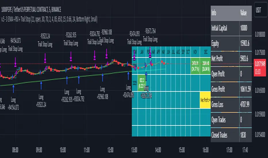
Codigo Trading 1.0📌Codigo Trading 1.0
This indicator strategically combines SuperTrend, multiple Exponential Moving Averages (EMAs), the Relative Strength Index (RSI), and the Average True Range (ATR) to offer clear entry and exit signals, as well as an in-depth view of market trends. Ideal for traders looking to optimize their operations with an all-in-one tool.
🔩How the Indicator Works:
This indicator relies on the interaction and confirmation of several key components to generate signals:
SuperTrend: Determines the primary trend direction. An uptrend SuperTrend signal (green line) indicates an upward trend, while a downtrend (red line) signals a downward trend. It also serves as a guide for setting Stop Loss and Take Profit levels.
EMAs: Includes EMAs of 10, 20, 55, 100, 200, and 325 periods. The relationship between the EMA 10 and EMA 20 is fundamental for confirming the strength and direction of movements. An EMA 10 above the EMA 20 suggests an uptrend, and vice versa. Longer EMAs act as dynamic support and resistance levels, offering a broader view of the market structure.
RSI: Used to identify overbought (RSI > 70/80) and oversold (RSI < 30/20) conditions, generating "Take Profit" alerts for potential trade closures.
ATR: Monitors market volatility to help you manage exits. ATR exit signals are triggered when volatility changes direction, indicating a possible exhaustion of the movement.
🗒️Entry and Exit Signals:
I designed specific alerts based on all the indicators I use in conjunction:
Long Entries: When SuperTrend is bullish and EMA 10 crosses above EMA 20.
Short Entries: When SuperTrend is bearish and EMA 10 crosses below EMA 20.
RSI Exits (Take Profit): Indicated by "TP" labels on the chart, when the RSI reaches extreme levels (overbought for longs, oversold for shorts).
EMA 20 Exits: When the price closes below EMA 20 (for longs) or above EMA 20 (for shorts).
ATR Exits: When the ATR changes direction, signaling a possible decrease in momentum.
📌Key Benefits:
Clarity in Trend: Quickly identifies market direction with SuperTrend and EMA alignment.
Strategic Entry and Exit Signals: Receive timely alerts to optimize your entry and exit points.
Assisted Trade Management: RSI and ATR help you consider when to take profits or exit a position.
Intuitive Visualization: Arrows, labels, and colored lines make analysis easy to interpret.
Disclaimer:
Trading in financial markets carries significant risks. This indicator is an analysis tool and should not be considered financial advice. Always conduct your own research and trade at your own risk.
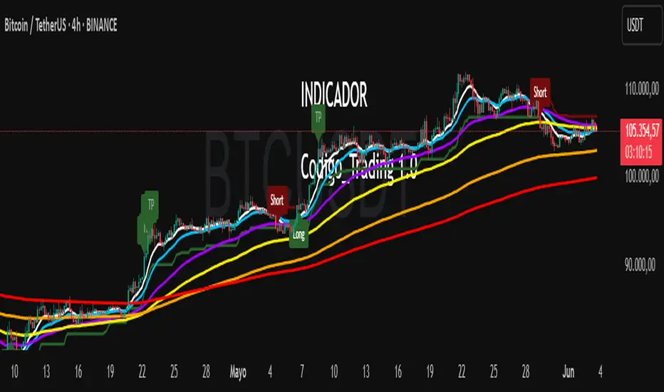
Crypto Scanner v4This guide explains a version 6 Pine Script that scans a user-provided list of cryptocurrency tokens to identify high probability tradable opportunities using several technical indicators. The script combines trend, momentum, and volume-based analyses to generate potential buying or selling signals, and it displays the results in a neatly formatted table with alerts for trading setups. Below is a detailed walkthrough of the script’s design, how traders can interpret its outputs, and recommendations for optimizing indicator inputs across different timeframes.
## Overview and Key Components
The script is designed to help traders assess multiple tokens by calculating several indicators for each one. The key components include:
- **Input Settings:**
- A comma-separated list of symbols to scan.
- Adjustable parameters for technical indicators such as ADX, RSI, MFI, and a custom Wave Trend indicator.
- Options to enable alerts and set update frequencies.
- **Indicator Calculations:**
- **ADX (Average Directional Index):** Measures trend strength. A value above the provided threshold indicates a strong trend, which is essential for validating momentum before entering a trade.
- **RSI (Relative Strength Index):** Helps determine overbought or oversold conditions. When the RSI is below the oversold level, it may present a buying opportunity, while an overbought condition (not explicitly part of this setup) could suggest selling.
- **MFI (Money Flow Index):** Similar in concept to RSI but incorporates volume, thus assessing buying and selling pressure. Values below the designated oversold threshold indicate potential undervaluation.
- **Wave Trend:** A custom indicator that calculates two components (WT1 and WT2); a crossover where WT1 moves from below to above WT2 (particularly near oversold levels) may signal a reversal and a potential entry point.
- **Scanning and Trading Zone:**
- The script identifies a *bullish setup* when the following conditions are met for a token:
- ADX exceeds the threshold (strong trend).
- Both RSI and MFI are below their oversold levels (indicating potential buying opportunities).
- A Wave Trend crossover confirms near-term reversal dynamics.
- A *trading zone* condition is also defined by specific ranges for ADX, RSI, MFI, and a limited difference between WT1 and WT2. This zone suggests that the token might be in a consolidation phase where even small moves may be significant.
- **Alerts and Table Reporting:**
- A table is generated, with each row corresponding to a token. The table contains columns for the symbol, ADX, RSI, MFI, WT1, WT2, and the trading zone status.
- Visual cues—such as different background colors—highlight tokens with a bullish setup or that are within the trading zone.
- Alerts are issued based on the detection of a bullish setup or entry into a trading zone. These alerts are limited per bar to avoid flooding the trader with notifications.
## How to Interpret the Indicator Outputs
Traders should use the indicator values as guidance, verifying them against their own analysis before making any trading decision. Here’s how to assess each output:
- **ADX:**
- **High values (above threshold):** Indicate strong trends. If other indicators confirm an oversold condition, a trader may consider a long position for a corrective reversal.
- **Low values:** Suggest that the market is not trending strongly, and caution should be taken when considering entry.
- **RSI and MFI:**
- **Below oversold levels:** These conditions are traditionally seen as signals that an asset is undervalued, potentially triggering a bounce.
- **Above typical resistance levels (not explicitly used here):** Would normally caution a trader against entering a long position.
- **Wave Trend (WT1 and WT2):**
- A crossover where WT1 moves upward above WT2 in an oversold environment can signal the beginning of a recovery or reversal, thereby reinforcing buy signals.
- **Trading Zone:**
- Being “in zone” means that the asset’s current values for ADX, RSI, MFI, and the closeness of the Wave Trend lines indicate a period of consolidation. This scenario might be suitable for both short-term scalping or as an early exit indicator, depending on further market analysis.
## Timeframe Optimization Input Table
Traders can optimize indicator inputs depending on the timeframe they use. The following table provides a set of recommended input values for various timeframes. These values are suggestions and should be adjusted based on market conditions and individual trading styles.
Timeframe ADX RSI MFI ADX RSI MFI WT Channel WT Average
5-min 10 10 10 20 30 20 7 15
15-min 12 12 12 22 30 20 9 18
1-hour 14 14 14 25 30 20 10 21
4-hour 16 16 16 27 30 20 12 24
1-day 18 18 18 30 30 20 14 28
Adjust these parameters directly in the script’s input settings to match the selected timeframe. For shorter timeframes (e.g., 5-min or 15-min), the shorter lengths help filter high-frequency noise. For longer timeframes (e.g., 1-day), longer input values may reduce false signals and capture more significant trends.
## Best Practices and Usage Tips
- **Token Limit:**
- Limit the number of tokens scanned to 10 per query line. If you need to scan more tokens, initiate a new query line. This helps manage screen real estate and ensures the table remains legible.
- **Confirming Signals:**
- Use this script as a starting point for identifying high potential trades. Each indicator’s output should be used to confirm your trading decision. Always cross-reference with additional technical analysis tools or market context.
- **Regular Review:**
- Since the script updates the table every few bars (as defined by the update frequency), review the table and alerts regularly. Market conditions change rapidly, so timely decisions are crucial.
## Conclusion
This Pine Script provides a comprehensive approach for scanning multiple cryptocurrencies using a combination of trend strength (ADX), momentum (RSI and MFI), and reversal signals (Wave Trend). By using the provided recommendation table for different timeframes and limiting the tokens to 20 per query line (with a maximum of four query lines), traders can streamline their scanning process and more effectively identify high probability tradable tokens. Ultimately, the outputs should be critically evaluated and combined with additional market research before executing any trades.

MEMA X-OL9+A. 5, 10, 20, 50 ema's
B. When the 10 goes below the 20 it has shades of red between the 10 and 20.
C. When there is a downward crossover, There will be a Red arrow pointing down.
D. When the 10 is moving closer (upward) towards the 20 it has orange shading. I use this to catch 10 over 20 crossovers.
E. When there is a crossover 10 over 20 it will shade green and have a gold arrow pointing upward. A little redundant, because you'll see the crossover from the shading.
F. Finally there will be smaller blue arrows that represent when there is a close of a candle, if it is lower than the prior candle.
All customizable and defaults should work.

M & W Checklistindicator to Validate & Grade M & W Patterns.
Indicator Inputs
Table Color Palette
• Position Valid : Positions the Valid Trade table on the chart.
• Position Grade : Positions the Grade table on the chart, hover over the Column 1 Row 1 for a description of the bands.
• Size: Text size for all tables.
• Text Color : Sets text color.
• Border Color : Sets the table border color for all tables.
• Background Color : Sets table backgroud color for all tables.
Valid Trade Table
Checkboxes to indicate if the trade is valid. Fail is displayed if unchecked, Pass if checked.
Grade Table
• S/R Level 1: distance between neckline and 1st resistance area in % of the total distance between neckline and take profit. This is not for road blocks but pivot points etc before the initial run up/down in price. I have this set to 30% , this means that if there is a pivot point between the neckline and 30% of the TP level I weight it negatively.
• S/R Level 2: distance between neckline and 1st resistance area in % of the total distance between neckline and take profit. This is not for road blocks but pivot points etc before the initial run up/down in price. I have this set to 50% , this means that if there is a pivot point between the neckline and 50% of the TP level 2 weight it negatively but less so than level 1.
• S/R Level 3: distance between neckline and 1st resistance area in % of the total distance between neckline and take profit. This is not for road blocks but pivot points etc before the initial run up/down in price. I have this set to 70% , this means that if there is a pivot point between the neckline and 70% of the TP level 3 weight it negatively but less so than level 1 & level 2.
• Checkboxes are self explanatory, they are binary options, all are weighted negatively if checked and are weighted positively if unchecked. Divergence values for weighting are neutral if unckecked & weighted positively if checked.
• The select options are neutral weighting if set to neutral , if set to For its weighted positive and set to Against weighted negatively.
Technical Specification of the Scoring and Band System
Overview
The scoring system is designed to evaluate a set of technical trade conditions, assigning weights to various criteria that influence the quality of the trade. The system calculates a total score based on both positive and negative conditions. Based on the final score, the system assigns a grade or band (A, B, or C) for positive scores, and a "Negative" label for negative scores.
Scoring System
The system calculates the score by evaluating a set of 12 conditions (gradeCondition1 to gradeCondition12). These conditions are manually input by the user via checkboxes or dropdowns in a technical indicator (written in Pine Script for TradingView). The score weights vary according to the relative importance of each condition.
Condition Breakdown and Weighting:
1. Divergences (GradeCondition1 & GradeCondition2):
◦ 1H Divergence: +5 points if condition is true.
◦ 4H Divergence: +10 points if condition is true (stronger weight than 1H).
2. Support/Resistance at Neckline (GradeCondition3):
◦ Negative if present: -15 points if true (carries significant negative weight).
3. RB near Entry (GradeCondition4):
◦ Very Negative: -20 points if true (this is a critical negative condition).
4. RB can Manage (GradeCondition5):
◦ Slightly Negative: -5 points if true.
5. Institutional Value Zones (GradeCondition6 to GradeCondition8):
◦ For the trade: +5 points.
◦ Against the trade: -5 points.
◦ Neutral: 0 points.
6. S/R between Neckline & Targets (GradeCondition9 to GradeCondition11):
◦ Level 1: -10 points if true, +7 points if false.
◦ Level 2: -7 points if true, +7 points if false.
◦ Level 3: -5 points if true, +7 points if false.
◦ Use fib tool or Gann Box to measure any S/R levels setup according to your preferences.
7. News Timing (GradeCondition12):
◦ News within 3 hours: -20 points if true (strong negative factor).
◦ No upcoming news: +10 points if false.
Scoring Calculation Formula:
totalScore = score1 + score2 + score3 + score4 + score5 + score6 + score7 + score8 + score9 + score10 + score11 + score12
Where:
• score1 to score12 represent the points derived from the conditions described above.
Coloring and Visual Feedback:
• Positive Scores: Displayed in green.
• Negative Scores: Displayed in red.
Band System
The Band System classifies the total score into different grades, depending on the final value of totalScore. This classification provides an intuitive ranking for trades, helping users quickly assess trade quality.
Band Classification:
• Band A: If the totalScore is 41 or more.
◦ Represents a highly favorable trade setup.
• Band B: If the totalScore is between 21 and 40.
◦ Represents a favorable trade setup with good potential.
• Band C: If the totalScore is between 1 and 20.
◦ Represents a trade setup that is acceptable but may have risks.
• Negative: If the totalScore is 0 or less.
◦ Represents a poor trade setup with significant risks or unfavorable conditions.
Band Calculation Logic (in Pine Script):
var string grade = ""
if (totalScore >= 41)
grade := "Band A"
else if (totalScore >= 21)
grade := "Band B"
else if (totalScore >= 1)
grade := "Band C"
else
grade := "Negative"
Technical Key Points:
• Highly Negative Conditions:
◦ The system penalizes certain conditions more heavily, especially those that suggest significant risks (e.g., News in less than 3 hours, RB near Entry).
• Positive Trade Conditions:
◦ Divergences, Institutional Value Zones in favor of the trade, and lack of significant nearby resistance all contribute positively to the score.
• Flexible System:
◦ The system can be adapted or fine-tuned by adjusting the weights of individual conditions according to trading preferences.
Use Case Example:
• If a trade has 1H and 4H Divergence, RB near Entry (negative), and no upcoming news:
◦ 1H Divergence: +5 points.
◦ 4H Divergence: +10 points.
◦ RB near Entry: -20 points.
◦ No news: +10 points.
◦ Total Score: 5 + 10 - 20 + 10 = 5 → Band C.
This modular and flexible scoring system allows traders to systematically evaluate trades and quickly gauge the trade's potential based on technical indicators
Summary:
Maximum Score: 61
Minimum Score: -97
These are the bounds of the score range based on the current logic of the script.

Grothendieck-Teichmüller Geometric SynthesisDskyz's Grothendieck-Teichmüller Geometric Synthesis (GTGS)
THEORETICAL FOUNDATION: A SYMPHONY OF GEOMETRIES
The 🎓 GTGS is built upon a revolutionary premise: that market dynamics can be modeled as geometric and topological structures. While not a literal academic implementation—such a task would demand computational power far beyond current trading platforms—it leverages core ideas from advanced mathematical theories as powerful analogies and frameworks for its algorithms. Each component translates an abstract concept into a practical market calculation, distinguishing GTGS by identifying deeper structural patterns rather than relying on standard statistical measures.
1. Grothendieck-Teichmüller Theory: Deforming Market Structure
The Theory : Studies symmetries and deformations of geometric objects, focusing on the "absolute" structure of mathematical spaces.
Indicator Analogy : The calculate_grothendieck_field function models price action as a "deformation" from its immediate state. Using the nth root of price ratios (math.pow(price_ratio, 1.0/prime)), it measures market "shape" stretching or compression, revealing underlying tensions and potential shifts.
2. Topos Theory & Sheaf Cohomology: From Local to Global Patterns
The Theory : A framework for assembling local properties into a global picture, with cohomology measuring "obstructions" to consistency.
Indicator Analogy : The calculate_topos_coherence function uses sine waves (math.sin) to represent local price "sections." Summing these yields a "cohomology" value, quantifying price action consistency. High values indicate coherent trends; low values signal conflict and uncertainty.
3. Tropical Geometry: Simplifying Complexity
The Theory : Transforms complex multiplicative problems into simpler, additive, piecewise-linear ones using min(a, b) for addition and a + b for multiplication.
Indicator Analogy : The calculate_tropical_metric function applies tropical_add(a, b) => math.min(a, b) to identify the "lowest energy" state among recent price points, pinpointing critical support levels non-linearly.
4. Motivic Cohomology & Non-Commutative Geometry
The Theory : Studies deep arithmetic and quantum-like properties of geometric spaces.
Indicator Analogy : The motivic_rank and spectral_triple functions compute weighted sums of historical prices to capture market "arithmetic complexity" and "spectral signature." Higher values reflect structured, harmonic price movements.
5. Perfectoid Spaces & Homotopy Type Theory
The Theory : Abstract fields dealing with p-adic numbers and logical foundations of mathematics.
Indicator Analogy : The perfectoid_conv and type_coherence functions analyze price convergence and path identity, assessing the "fractal dust" of price differences and price path cohesion, adding fractal and logical analysis.
The Combination is Key : No single theory dominates. GTGS ’s Unified Field synthesizes all seven perspectives into a comprehensive score, ensuring signals reflect deep structural alignment across mathematical domains.
🎛️ INPUTS: CONFIGURING THE GEOMETRIC ENGINE
The GTGS offers a suite of customizable inputs, allowing traders to tailor its behavior to specific timeframes, market sectors, and trading styles. Below is a detailed breakdown of key input groups, their functionality, and optimization strategies, leveraging provided tooltips for precision.
Grothendieck-Teichmüller Theory Inputs
🧬 Deformation Depth (Absolute Galois) :
What It Is : Controls the depth of Galois group deformations analyzed in market structure.
How It Works : Measures price action deformations under automorphisms of the absolute Galois group, capturing market symmetries.
Optimization :
Higher Values (15-20) : Captures deeper symmetries, ideal for major trends in swing trading (4H-1D).
Lower Values (3-8) : Responsive to local deformations, suited for scalping (1-5min).
Timeframes :
Scalping (1-5min) : 3-6 for quick local shifts.
Day Trading (15min-1H) : 8-12 for balanced analysis.
Swing Trading (4H-1D) : 12-20 for deep structural trends.
Sectors :
Stocks : Use 8-12 for stable trends.
Crypto : 3-8 for volatile, short-term moves.
Forex : 12-15 for smooth, cyclical patterns.
Pro Tip : Increase in trending markets to filter noise; decrease in choppy markets for sensitivity.
🗼 Teichmüller Tower Height :
What It Is : Determines the height of the Teichmüller modular tower for hierarchical pattern detection.
How It Works : Builds modular levels to identify nested market patterns.
Optimization :
Higher Values (6-8) : Detects complex fractals, ideal for swing trading.
Lower Values (2-4) : Focuses on primary patterns, faster for scalping.
Timeframes :
Scalping : 2-3 for speed.
Day Trading : 4-5 for balanced patterns.
Swing Trading : 5-8 for deep fractals.
Sectors :
Indices : 5-8 for robust, long-term patterns.
Crypto : 2-4 for rapid shifts.
Commodities : 4-6 for cyclical trends.
Pro Tip : Higher towers reveal hidden fractals but may slow computation; adjust based on hardware.
🔢 Galois Prime Base :
What It Is : Sets the prime base for Galois field computations.
How It Works : Defines the field extension characteristic for market analysis.
Optimization :
Prime Characteristics :
2 : Binary markets (up/down).
3 : Ternary states (bull/bear/neutral).
5 : Pentagonal symmetry (Elliott waves).
7 : Heptagonal cycles (weekly patterns).
11,13,17,19 : Higher-order patterns.
Timeframes :
Scalping/Day Trading : 2 or 3 for simplicity.
Swing Trading : 5 or 7 for wave or cycle detection.
Sectors :
Forex : 5 for Elliott wave alignment.
Stocks : 7 for weekly cycle consistency.
Crypto : 3 for volatile state shifts.
Pro Tip : Use 7 for most markets; 5 for Elliott wave traders.
Topos Theory & Sheaf Cohomology Inputs
🏛️ Temporal Site Size :
What It Is : Defines the number of time points in the topological site.
How It Works : Sets the local neighborhood for sheaf computations, affecting cohomology smoothness.
Optimization :
Higher Values (30-50) : Smoother cohomology, better for trends in swing trading.
Lower Values (5-15) : Responsive, ideal for reversals in scalping.
Timeframes :
Scalping : 5-10 for quick responses.
Day Trading : 15-25 for balanced analysis.
Swing Trading : 25-50 for smooth trends.
Sectors :
Stocks : 25-35 for stable trends.
Crypto : 5-15 for volatility.
Forex : 20-30 for smooth cycles.
Pro Tip : Match site size to your average holding period in bars for optimal coherence.
📐 Sheaf Cohomology Degree :
What It Is : Sets the maximum degree of cohomology groups computed.
How It Works : Higher degrees capture complex topological obstructions.
Optimization :
Degree Meanings :
1 : Simple obstructions (basic support/resistance).
2 : Cohomological pairs (double tops/bottoms).
3 : Triple intersections (complex patterns).
4-5 : Higher-order structures (rare events).
Timeframes :
Scalping/Day Trading : 1-2 for simplicity.
Swing Trading : 3 for complex patterns.
Sectors :
Indices : 2-3 for robust patterns.
Crypto : 1-2 for rapid shifts.
Commodities : 3-4 for cyclical events.
Pro Tip : Degree 3 is optimal for most trading; higher degrees for research or rare event detection.
🌐 Grothendieck Topology :
What It Is : Chooses the Grothendieck topology for the site.
How It Works : Affects how local data integrates into global patterns.
Optimization :
Topology Characteristics :
Étale : Finest topology, captures local-global principles.
Nisnevich : A1-invariant, good for trends.
Zariski : Coarse but robust, filters noise.
Fpqc : Faithfully flat, highly sensitive.
Sectors :
Stocks : Zariski for stability.
Crypto : Étale for sensitivity.
Forex : Nisnevich for smooth trends.
Indices : Zariski for robustness.
Timeframes :
Scalping : Étale for precision.
Swing Trading : Nisnevich or Zariski for reliability.
Pro Tip : Start with Étale for precision; switch to Zariski in noisy markets.
Unified Field Configuration Inputs
⚛️ Field Coupling Constant :
What It Is : Sets the interaction strength between geometric components.
How It Works : Controls signal amplification in the unified field equation.
Optimization :
Higher Values (0.5-1.0) : Strong coupling, amplified signals for ranging markets.
Lower Values (0.001-0.1) : Subtle signals for trending markets.
Timeframes :
Scalping : 0.5-0.8 for quick, strong signals.
Swing Trading : 0.1-0.3 for trend confirmation.
Sectors :
Crypto : 0.5-1.0 for volatility.
Stocks : 0.1-0.3 for stability.
Forex : 0.3-0.5 for balance.
Pro Tip : Default 0.137 (fine structure constant) is a balanced starting point; adjust up in choppy markets.
📐 Geometric Weighting Scheme :
What It Is : Determines the framework for combining geometric components.
How It Works : Adjusts emphasis on different mathematical structures.
Optimization :
Scheme Characteristics :
Canonical : Equal weighting, balanced.
Derived : Emphasizes higher-order structures.
Motivic : Prioritizes arithmetic properties.
Spectral : Focuses on frequency domain.
Sectors :
Stocks : Canonical for balance.
Crypto : Spectral for volatility.
Forex : Derived for structured moves.
Indices : Motivic for arithmetic cycles.
Timeframes :
Day Trading : Canonical or Derived for flexibility.
Swing Trading : Motivic for long-term cycles.
Pro Tip : Start with Canonical; experiment with Spectral in volatile markets.
Dashboard and Visual Configuration Inputs
📋 Show Enhanced Dashboard, 📏 Size, 📍 Position :
What They Are : Control dashboard visibility, size, and placement.
How They Work : Display key metrics like Unified Field , Resonance , and Signal Quality .
Optimization :
Scalping : Small size, Bottom Right for minimal chart obstruction.
Swing Trading : Large size, Top Right for detailed analysis.
Sectors : Universal across markets; adjust size based on screen setup.
Pro Tip : Use Large for analysis, Small for live trading.
📐 Show Motivic Cohomology Bands, 🌊 Morphism Flow, 🔮 Future Projection, 🔷 Holographic Mesh, ⚛️ Spectral Flow :
What They Are : Toggle visual elements representing mathematical calculations.
How They Work : Provide intuitive representations of market dynamics.
Optimization :
Timeframes :
Scalping : Enable Morphism Flow and Spectral Flow for momentum.
Swing Trading : Enable all for comprehensive analysis.
Sectors :
Crypto : Emphasize Morphism Flow and Future Projection for volatility.
Stocks : Focus on Cohomology Bands for stable trends.
Pro Tip : Disable non-essential visuals in fast markets to reduce clutter.
🌫️ Field Transparency, 🔄 Web Recursion Depth, 🎨 Mesh Color Scheme :
What They Are : Adjust visual clarity, complexity, and color.
How They Work : Enhance interpretability of visual elements.
Optimization :
Transparency : 30-50 for balanced visibility; lower for analysis.
Recursion Depth : 6-8 for balanced detail; lower for older hardware.
Color Scheme :
Purple/Blue : Analytical focus.
Green/Orange : Trading momentum.
Pro Tip : Use Neon Purple for deep analysis; Neon Green for active trading.
⏱️ Minimum Bars Between Signals :
What It Is : Minimum number of bars required between consecutive signals.
How It Works : Prevents signal clustering by enforcing a cooldown period.
Optimization :
Higher Values (10-20) : Fewer signals, avoids whipsaws, suited for swing trading.
Lower Values (0-5) : More responsive, allows quick reversals, ideal for scalping.
Timeframes :
Scalping : 0-2 bars for rapid signals.
Day Trading : 3-5 bars for balance.
Swing Trading : 5-10 bars for stability.
Sectors :
Crypto : 0-3 for volatility.
Stocks : 5-10 for trend clarity.
Forex : 3-7 for cyclical moves.
Pro Tip : Increase in choppy markets to filter noise.
Hardcoded Parameters
Tropical, Motivic, Spectral, Perfectoid, Homotopy Inputs : Fixed to optimize performance but influence calculations (e.g., tropical_degree=4 for support levels, perfectoid_prime=5 for convergence).
Optimization : Experiment with codebase modifications if advanced customization is needed, but defaults are robust across markets.
🎨 ADVANCED VISUAL SYSTEM: TRADING IN A GEOMETRIC UNIVERSE
The GTTMTSF ’s visuals are direct representations of its mathematics, designed for intuitive and precise trading decisions.
Motivic Cohomology Bands :
What They Are : Dynamic bands ( H⁰ , H¹ , H² ) representing cohomological support/resistance.
Color & Meaning : Colors reflect energy levels ( H⁰ tightest, H² widest). Breaks into H¹ signal momentum; H² touches suggest reversals.
How to Trade : Use for stop-loss/profit-taking. Band bounces with Dashboard confirmation are high-probability setups.
Morphism Flow (Webbing) :
What It Is : White particle streams visualizing market momentum.
Interpretation : Dense flows indicate strong trends; sparse flows signal consolidation.
How to Trade : Follow dominant flow direction; new flows post-consolidation signal trend starts.
Future Projection Web (Fractal Grid) :
What It Is : Fibonacci-period fractal projections of support/resistance.
Color & Meaning : Three-layer lines (white shadow, glow, colored quantum) with labels showing price, topological class, anomaly strength (φ), resonance (ρ), and obstruction ( H¹ ). ⚡ marks extreme anomalies.
How to Trade : Target ⚡/● levels for entries/exits. High-anomaly levels with weakening Unified Field are reversal setups.
Holographic Mesh & Spectral Flow :
What They Are : Visuals of harmonic interference and spectral energy.
How to Trade : Bright mesh nodes or strong Spectral Flow warn of building pressure before price movement.
📊 THE GEOMETRIC DASHBOARD: YOUR MISSION CONTROL
The Dashboard translates complex mathematics into actionable intelligence.
Unified Field & Signals :
FIELD : Master value (-10 to +10), synthesizing all geometric components. Extreme readings (>5 or <-5) signal structural limits, often preceding reversals or continuations.
RESONANCE : Measures harmony between geometric field and price-volume momentum. Positive amplifies bullish moves; negative amplifies bearish moves.
SIGNAL QUALITY : Confidence meter rating alignment. Trade only STRONG or EXCEPTIONAL signals for high-probability setups.
Geometric Components :
What They Are : Breakdown of seven mathematical engines.
How to Use : Watch for convergence. A strong Unified Field is reliable when components (e.g., Grothendieck , Topos , Motivic ) align. Divergence warns of trend weakening.
Signal Performance :
What It Is : Tracks indicator signal performance.
How to Use : Assesses real-time performance to build confidence and understand system behavior.
🚀 DEVELOPMENT & UNIQUENESS: BEYOND CONVENTIONAL ANALYSIS
The GTTMTSF was developed to analyze markets as evolving geometric objects, not statistical time-series.
Why This Is Unlike Anything Else :
Theoretical Depth : Uses geometry and topology, identifying patterns invisible to statistical tools.
Holistic Synthesis : Integrates seven deep mathematical frameworks into a cohesive Unified Field .
Creative Implementation : Translates PhD-level mathematics into functional Pine Script , blending theory and practice.
Immersive Visualization : Transforms charts into dynamic geometric landscapes for intuitive market understanding.
The GTTMTSF is more than an indicator; it’s a new lens for viewing markets, for traders seeking deeper insight into hidden order within chaos.
" Where there is matter, there is geometry. " - Johannes Kepler
— Dskyz , Trade with insight. Trade with anticipation.
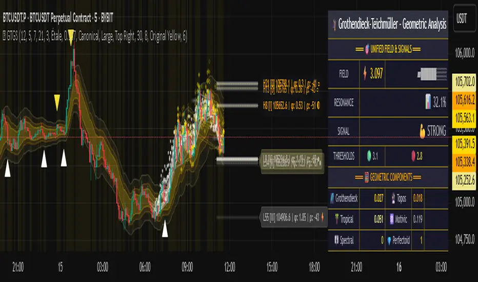
4 SMAs & Inside Bar (Colored)SMAs and Inside Bar strategy is very common as far as Technical analysis is concern. This script is a combination of 10-20-50-200 SMA and Inside Bar Candle Identification.
SMA Crossover:
4 SMAs (10, 20, 50 & 200) are combined here in one single indicator.
Crossover signal for Buy as "B" will be shown in the chart if SMA 10 is above 20 & 50 and SMA 20 is above 50.
Crossover signal for Sell as "S" will be shown in the chart if SMA 10 is below 20 & 50 and SMA 20 is below 50.
Inside Bar Identification:
This is to simply identify if there is a inside bar candle. The logic is very simple - High of the previous candle should be higher than current candle and low of the previous candle should be lower than the current candle.
If the previous candle is red, the following candle would be Yellow - which may give some bullish view in most of the cases but not always
If the previous candle is green, the following candle would be Black - which may give some bearish view in most of the cases but not always
Be Cautious when you see alternate yellow and black candle, it may give move on the both side
Please comment if you have any interesting ideas to improve this indicator.
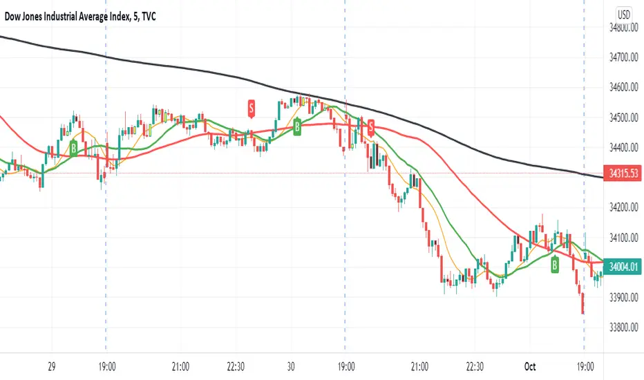
Pivot S/R with Volatility Filter## *📌 Indicator Purpose*
This indicator identifies *key support/resistance levels* using pivot points while also:
✅ Detecting *high-volume liquidity traps* (stop hunts)
✅ Filtering insignificant pivots via *ATR (Average True Range) volatility*
✅ Tracking *test counts and breakouts* to measure level strength
---
## *⚙ SETTINGS – Detailed Breakdown*
### *1️⃣ ◆ General Settings*
#### *🔹 Pivot Length*
- *Purpose:* Determines how many bars to analyze when identifying pivots.
- *Usage:*
- *Low values (5-20):* More pivots, better for scalping.
- *High values (50-200):* Fewer but stronger levels for swing trading.
- *Example:*
- Pivot Length = 50 → Only the most significant highs/lows over 50 bars are marked.
#### *🔹 Test Threshold (Max Test Count)*
- *Purpose:* Sets how many times a level can be tested before being invalidated.
- *Example:*
- Test Threshold = 3 → After 3 tests, the level is ignored (likely to break).
#### *🔹 Zone Range*
- *Purpose:* Creates a price buffer around pivots (±0.001 by default).
- *Why?* Markets often respect "zones" rather than exact prices.
---
### *2️⃣ ◆ Volatility Filter (ATR)*
#### *🔹 ATR Period*
- *Purpose:* Smoothing period for Average True Range calculation.
- *Default:* 14 (standard for volatility measurement).
#### *🔹 ATR Multiplier (Min Move)*
- *Purpose:* Requires pivots to show *meaningful price movement*.
- *Formula:* Min Move = ATR × Multiplier
- *Example:*
- ATR = 10 pips, Multiplier = 1.5 → Only pivots with *15+ pip swings* are valid.
#### *🔹 Show ATR Filter Info*
- Displays current ATR and minimum move requirements on the chart.
---
### *3️⃣ ◆ Volume Analysis*
#### *🔹 Volume Change Threshold (%)*
- *Purpose:* Filters for *unusual volume spikes* (institutional activity).
- *Example:*
- Threshold = 1.2 → Requires *120% of average volume* to confirm signals.
#### *🔹 Volume MA Period*
- *Purpose:* Lookback period for "normal" volume calculation.
---
### *4️⃣ ◆ Wick Analysis*
#### *🔹 Wick Length Threshold (Ratio)*
- *Purpose:* Ensures rejection candles have *long wicks* (strong reversals).
- *Formula:* Wick Ratio = (Upper Wick + Lower Wick) / Candle Range
- *Example:*
- Threshold = 0.6 → 60% of the candle must be wicks.
#### *🔹 Min Wick Size (ATR %)*
- *Purpose:* Filters out small wicks in volatile markets.
- *Example:*
- ATR = 20 pips, MinWickSize = 1% → Wicks under *0.2 pips* are ignored.
---
### *5️⃣ ◆ Display Settings*
- *Show Zones:* Toggles support/resistance shaded areas.
- *Show Traps:* Highlights liquidity traps (▲/▼ symbols).
- *Show Tests:* Displays how many times levels were tested.
- *Zone Transparency:* Adjusts opacity of zones.
---
## *🎯 Practical Use Cases*
### *1️⃣ Liquidity Trap Detection*
- *Scenario:* Price spikes *above resistance* then reverses sharply.
- *Requirements:*
- Long wick (Wick Ratio > 0.6)
- High volume (Volume > Threshold)
- *Outcome:* *Short Trap* signal (▼) appears.
### *2️⃣ Strong Support Level*
- *Scenario:* Price bounces *3 times* from the same level.
- *Indicator Action:*
- Labels the level with test count (3/5 = 3 tests out of max 5).
- Turns *red* if broken (Break Count > 0).
Deep Dive: How This Indicator Works*
This indicator combines *four professional trading concepts* into one powerful tool:
1. *Classic Pivot Point Theory*
- Identifies swing highs/lows where price previously reversed
- Unlike basic pivot indicators, ours uses *confirmed pivots only* (filtered by ATR)
2. *Volume-Weighted Validation*
- Requires unusual trading volume to confirm levels
- Filters out "phantom" levels with low participation
3. *ATR Volatility Filtering*
- Eliminates insignificant price swings in choppy markets
- Ensures only meaningful levels are plotted
4. *Liquidity Trap Detection*
- Spots institutional stop hunts where markets fake out traders
- Uses wick analysis + volume spikes for high-probability signals
---
## *📊 Parameter Encyclopedia (Expanded)*
### *1️⃣ Pivot Engine Settings*
#### *Pivot Length (50)*
- *What It Does:*
Determines how many bars to analyze when searching for swing highs/lows.
- *Professional Adjustment Guide:*
| Trading Style | Recommended Value | Why? |
|--------------|------------------|------|
| Scalping | 10-20 | Captures short-term levels |
| Day Trading | 30-50 | Balanced approach |
| Swing Trading| 50-200 | Focuses on major levels |
- *Real Market Example:*
On NASDAQ 5-minute chart:
- Length=20: Identifies levels holding for ~2 hours
- Length=50: Finds levels respected for entire trading day
#### *Test Threshold (5)*
- *Advanced Insight:*
Institutions often test levels 3-5 times before breaking them. This setting mimics the "probe and push" strategy used by smart money.
- *Psychology Behind It:*
Retail traders typically give up after 2-3 tests, while institutions keep testing until stops are run.
---
### *2️⃣ Volatility Filter System*
#### *ATR Multiplier (1.0)*
- *Professional Formula:*
Minimum Valid Swing = ATR(14) × Multiplier
- *Market-Specific Recommendations:*
| Market Type | Optimal Multiplier |
|------------------|--------------------|
| Forex Majors | 0.8-1.2 |
| Crypto (BTC/ETH) | 1.5-2.5 |
| SP500 Stocks | 1.0-1.5 |
- *Why It Matters:*
In EUR/USD (ATR=10 pips):
- Multiplier=1.0 → Requires 10 pip swings
- Multiplier=1.5 → Requires 15 pip swings (fewer but higher quality levels)
---
### *3️⃣ Volume Confirmation System*
#### *Volume Threshold (1.2)*
- *Institutional Benchmark:*
- 1.2x = Moderate institutional interest
- 1.5x+ = Strong smart money activity
- *Volume Spike Case Study:*
*Before Apple Earnings:*
- Normal volume: 2M shares
- Spike threshold (1.2): 2.4M shares
- Actual volume: 3.1M shares → STRONG confirmation
---
### *4️⃣ Liquidity Trap Detection*
#### *Wick Analysis System*
- *Two-Filter Verification:*
1. *Wick Ratio (0.6):*
- Ensures majority of candle shows rejection
- Formula: (UpperWick + LowerWick) / Total Range > 0.6
2. *Min Wick Size (1% ATR):*
- Prevents false signals in flat markets
- Example: ATR=20 pips → Min wick=0.2 pips
- *Trap Identification Flowchart:*
Price Enters Zone →
Spikes Beyond Level →
Shows Long Wick →
Volume > Threshold →
TRAP CONFIRMED
---
## *💡 Master-Level Usage Techniques*
### *Institutional Order Flow Analysis*
1. *Step 1:* Identify pivot levels with ≥3 tests
2. *Step 2:* Watch for volume contraction near levels
3. *Step 3:* Enter when trap signal appears with:
- Wick > 2×ATR
- Volume > 1.5× average
### *Multi-Timeframe Confirmation*
1. *Higher TF:* Find weekly/monthly pivots
2. *Lower TF:* Use this indicator for precise entries
3. *Example:*
- Weekly pivot at $180
- 4H shows liquidity trap → High-probability reversal
---
## *⚠ Critical Mistakes to Avoid*
1. *Using Default Settings Everywhere*
- Crude oil needs higher ATR multiplier than bonds
2. *Ignoring Trap Context*
- Traps work best at:
- All-time highs/lows
- Major psychological numbers (00/50 levels)
3. *Overlooking Cumulative Volume*
- Check if volume is building over multiple tests

Donchian Quest Research// =================================
Trend following strategy.
// =================================
Strategy uses two channels. One channel - for opening trades. Second channel - for closing.
Channel is similar to Donchian channel, but uses Close prices (not High/Low). That helps don't react to wicks of volatile candles (“stop hunting”). In most cases openings occur earlier than in Donchian channel. Closings occur only for real breakout.
// =================================
Strategy waits for beginning of trend - when price breakout of channel. Default length of both channels = 50 candles.
Conditions of trading:
- Open Long: If last Close = max Close for 50 closes.
- Close Long: If last Close = min Close for 50 closes.
- Open Short: If last Close = min Close for 50 closes.
- Close Short: If last Close = max Close for 50 closes.
// =================================
Color of lines:
- black - channel for opening trade.
- red - channel for closing trade.
- yellow - entry price.
- fuchsia - stoploss and breakeven.
- vertical green - go Long.
- vertical red - go Short.
- vertical gray - close in end, don't trade anymore.
// =================================
Order size calculated with ATR and volatility.
You can't trade 1 contract in BTC and 1 contract in XRP - for example. They have different price and volatility, so 1 contract BTC not equal 1 contract XRP.
Script uses universal calculation for every market. It is based on:
- Risk - USD sum you ready to loss in one trade. It calculated as percent of Equity.
- ATR indicator - measurement of volatility.
With default setting your stoploss = 0.5 percent of equity:
- If initial capital is 1000 USD and used parameter "Permit stop" - loss will be 5 USD (0.5 % of equity).
- If your Equity rises to 2000 USD and used parameter "Permit stop"- loss will be 10 USD (0.5 % of Equity).
// =================================
This Risk works only if you enable “Permit stop” parameter in Settings.
If this parameter disabled - strategy works as reversal strategy:
⁃ If close Long - channel border works as stoploss and momentarily go Short.
⁃ If close Short - channel border works as stoploss and momentarily go Long.
Channel borders changed dynamically. So sometime your loss will be greater than ‘Risk %’. Sometime - less than ‘Risk %’.
If this parameter enabled - maximum loss always equal to 'Risk %'. This parameter also include breakeven: if profit % = Risk %, then move stoploss to entry price.
// =================================
Like all trend following strategies - it works only in trend conditions. If no trend - slowly bleeding. There is no special additional indicator to filter trend/notrend. You need to trade every signal of strategy.
Strategy gives many losses:
⁃ 30 % of trades will close with profit.
⁃ 70 % of trades will close with loss.
⁃ But profit from 30% will be much greater than loss from 70 %.
Your task - patiently wait for it and don't use risky setting for position sizing.
// =================================
Recommended timeframe - Daily.
// =================================
Trend can vary in lengths. Selecting length of channels determine which trend you will be hunting:
⁃ 20/10 - from several days to several weeks.
⁃ 20/20 or 50/20 - from several weeks to several months.
⁃ 50/50 or 100/50 or 100/100 - from several months to several years.
// =================================
Inputs (Settings):
- Length: length of channel for trade opening/closing. You can choose 20/10, 20/20, 50/20, 50/50, 100/50, 100/100. Default value: 50/50.
- Permit Long / Permit short: Longs are most profitable for this strategy. You can disable Shorts and enable Longs only. Default value: permit all directions.
- Risk % of Equity: for position sizing used Equity percent. Don't use values greater than 5 % - it's risky. Default value: 0.5%.
⁃ ATR multiplier: this multiplier moves stoploss up or down. Big multiplier = small size of order, small profit, stoploss far from entry, low chance of stoploss. Small multiplier = big size of order, big profit, stop near entry, high chance of stoploss. Default value: 2.
- ATR length: number of candles to calculate ATR indicator. It used for order size and stoploss. Default value: 20.
- Close in end - to close active trade in the end (and don't trade anymore) or leave it open. You can see difference in Strategy Tester. Default value: don’t close.
- Permit stop: use stop or go reversal. Default value: without stop, reversal strategy.
// =================================
Properties (Settings):
- Initial capital - 1000 USD.
- Script don't uses 'Order size' - you need to change 'Risk %' in Inputs instead.
- Script don't uses 'Pyramiding'.
- 'Commission' 0.055 % and 'Slippage' 0 - this parameters are for crypto exchanges with perpetual contracts (for example Bybit). If use on other markets - set it accordingly to your exchange parameters.
// =================================
Big dataset used for chart - 'BITCOIN ALL TIME HISTORY INDEX'. It gives enough trades to understand logic of script. It have several good trends.
// =================================
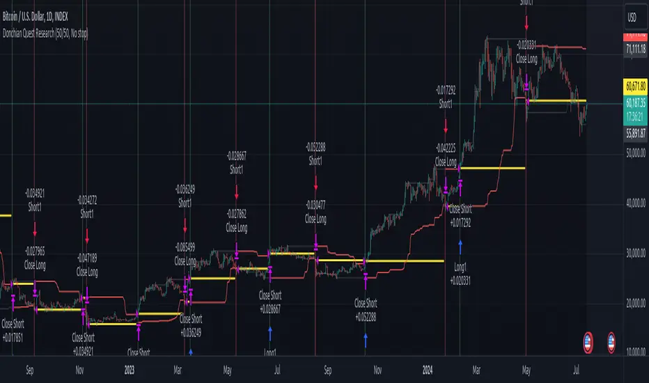
Langlands-Operadic Möbius Vortex (LOMV)Langlands-Operadic Möbius Vortex (LOMV)
Where Pure Mathematics Meets Market Reality
A Revolutionary Synthesis of Number Theory, Category Theory, and Market Dynamics
🎓 THEORETICAL FOUNDATION
The Langlands-Operadic Möbius Vortex represents a groundbreaking fusion of three profound mathematical frameworks that have never before been combined for market analysis:
The Langlands Program: Harmonic Analysis in Markets
Developed by Robert Langlands (Fields Medal recipient), the Langlands Program creates bridges between number theory, algebraic geometry, and harmonic analysis. In our indicator:
L-Function Implementation:
- Utilizes the Möbius function μ(n) for weighted price analysis
- Applies Riemann zeta function convergence principles
- Calculates quantum harmonic resonance between -2 and +2
- Measures deep mathematical patterns invisible to traditional analysis
The L-Function core calculation employs:
L_sum = Σ(return_val × μ(n) × n^(-s))
Where s is the critical strip parameter (0.5-2.5), controlling mathematical precision and signal smoothness.
Operadic Composition Theory: Multi-Strategy Democracy
Category theory and operads provide the mathematical framework for composing multiple trading strategies into a unified signal. This isn't simple averaging - it's mathematical composition using:
Strategy Composition Arity (2-5 strategies):
- Momentum analysis via RSI transformation
- Mean reversion through Bollinger Band mathematics
- Order Flow Polarity Index (revolutionary T3-smoothed volume analysis)
- Trend detection using Directional Movement
- Higher timeframe momentum confirmation
Agreement Threshold System: Democratic voting where strategies must reach consensus before signal generation. This prevents false signals during market uncertainty.
Möbius Function: Number Theory in Action
The Möbius function μ(n) forms the mathematical backbone:
- μ(n) = 1 if n is a square-free positive integer with even number of prime factors
- μ(n) = -1 if n is a square-free positive integer with odd number of prime factors
- μ(n) = 0 if n has a squared prime factor
This creates oscillating weights that reveal hidden market periodicities and harmonic structures.
🔧 COMPREHENSIVE INPUT SYSTEM
Langlands Program Parameters
Modular Level N (5-50, default 30):
Primary lookback for quantum harmonic analysis. Optimized by timeframe:
- Scalping (1-5min): 15-25
- Day Trading (15min-1H): 25-35
- Swing Trading (4H-1D): 35-50
- Asset-specific: Crypto 15-25, Stocks 30-40, Forex 35-45
L-Function Critical Strip (0.5-2.5, default 1.5):
Controls Riemann zeta convergence precision:
- Higher values: More stable, smoother signals
- Lower values: More reactive, catches quick moves
- High frequency: 0.8-1.2, Medium: 1.3-1.7, Low: 1.8-2.3
Frobenius Trace Period (5-50, default 21):
Galois representation lookback for price-volume correlation:
- Measures harmonic relationships in market flows
- Scalping: 8-15, Day Trading: 18-25, Swing: 25-40
HTF Multi-Scale Analysis:
Higher timeframe context prevents trading against major trends:
- Provides market bias and filters signals
- Improves win rates by 15-25% through trend alignment
Operadic Composition Parameters
Strategy Composition Arity (2-5, default 4):
Number of algorithms composed for final signal:
- Conservative: 4-5 strategies (higher confidence)
- Moderate: 3-4 strategies (balanced approach)
- Aggressive: 2-3 strategies (more frequent signals)
Category Agreement Threshold (2-5, default 3):
Democratic voting minimum for signal generation:
- Higher agreement: Fewer but higher quality signals
- Lower agreement: More signals, potential false positives
Swiss-Cheese Mixing (0.1-0.5, default 0.382):
Golden ratio φ⁻¹ based blending of trend factors:
- 0.382 is φ⁻¹, optimal for natural market fractals
- Higher values: Stronger trend following
- Lower values: More contrarian signals
OFPI Configuration:
- OFPI Length (5-30, default 14): Order Flow calculation period
- T3 Smoothing (3-10, default 5): Advanced exponential smoothing
- T3 Volume Factor (0.5-1.0, default 0.7): Smoothing aggressiveness control
Unified Scoring System
Component Weights (sum ≈ 1.0):
- L-Function Weight (0.1-0.5, default 0.3): Mathematical harmony emphasis
- Galois Rank Weight (0.1-0.5, default 0.2): Market structure complexity
- Operadic Weight (0.1-0.5, default 0.3): Multi-strategy consensus
- Correspondence Weight (0.1-0.5, default 0.2): Theory-practice alignment
Signal Threshold (0.5-10.0, default 5.0):
Quality filter producing:
- 8.0+: EXCEPTIONAL signals only
- 6.0-7.9: STRONG signals
- 4.0-5.9: MODERATE signals
- 2.0-3.9: WEAK signals
🎨 ADVANCED VISUAL SYSTEM
Multi-Dimensional Quantum Aura Bands
Five-layer resonance field showing market energy:
- Colors: Theme-matched gradients (Quantum purple, Holographic cyan, etc.)
- Expansion: Dynamic based on score intensity and volatility
- Function: Multi-timeframe support/resistance zones
Morphism Flow Portals
Category theory visualization showing market topology:
- Green/Cyan Portals: Bullish mathematical flow
- Red/Orange Portals: Bearish mathematical flow
- Size/Intensity: Proportional to signal strength
- Recursion Depth (1-8): Nested patterns for flow evolution
Fractal Grid System
Dynamic support/resistance with projected L-Scores:
- Multiple Timeframes: 10, 20, 30, 40, 50-period highs/lows
- Smart Spacing: Prevents level overlap using ATR-based minimum distance
- Projections: Estimated signal scores when price reaches levels
- Usage: Precise entry/exit timing with mathematical confirmation
Wick Pressure Analysis
Rejection level prediction using candle mathematics:
- Upper Wicks: Selling pressure zones (purple/red lines)
- Lower Wicks: Buying pressure zones (purple/green lines)
- Glow Intensity (1-8): Visual emphasis and line reach
- Application: Confluence with fractal grid creates high-probability zones
Regime Intensity Heatmap
Background coloring showing market energy:
- Black/Dark: Low activity, range-bound markets
- Purple Glow: Building momentum and trend development
- Bright Purple: High activity, strong directional moves
- Calculation: Combines trend, momentum, volatility, and score intensity
Six Professional Themes
- Quantum: Purple/violet for general trading and mathematical focus
- Holographic: Cyan/magenta optimized for cryptocurrency markets
- Crystalline: Blue/turquoise for conservative, stability-focused trading
- Plasma: Gold/magenta for high-energy volatility trading
- Cosmic Neon: Bright neon colors for maximum visibility and aggressive trading
📊 INSTITUTIONAL-GRADE DASHBOARD
Unified AI Score Section
- Total Score (-10 to +10): Primary decision metric
- >5: Strong bullish signals
- <-5: Strong bearish signals
- Quality ratings: EXCEPTIONAL > STRONG > MODERATE > WEAK
- Component Analysis: Individual L-Function, Galois, Operadic, and Correspondence contributions
Order Flow Analysis
Revolutionary OFPI integration:
- OFPI Value (-100% to +100%): Real buying vs selling pressure
- Visual Gauge: Horizontal bar chart showing flow intensity
- Momentum Status: SHIFTING, ACCELERATING, STRONG, MODERATE, or WEAK
- Trading Application: Flow shifts often precede major moves
Signal Performance Tracking
- Win Rate Monitoring: Real-time success percentage with emoji indicators
- Signal Count: Total signals generated for frequency analysis
- Current Position: LONG, SHORT, or NONE with P&L tracking
- Volatility Regime: HIGH, MEDIUM, or LOW classification
Market Structure Analysis
- Möbius Field Strength: Mathematical field oscillation intensity
- CHAOTIC: High complexity, use wider stops
- STRONG: Active field, normal position sizing
- MODERATE: Balanced conditions
- WEAK: Low activity, consider smaller positions
- HTF Trend: Higher timeframe bias (BULL/BEAR/NEUTRAL)
- Strategy Agreement: Multi-algorithm consensus level
Position Management
When in trades, displays:
- Entry Price: Original signal price
- Current P&L: Real-time percentage with risk level assessment
- Duration: Bars in trade for timing analysis
- Risk Level: HIGH/MEDIUM/LOW based on current exposure
🚀 SIGNAL GENERATION LOGIC
Balanced Long/Short Architecture
The indicator generates signals through multiple convergent pathways:
Long Entry Conditions:
- Score threshold breach with algorithmic agreement
- Strong bullish order flow (OFPI > 0.15) with positive composite signal
- Bullish pattern recognition with mathematical confirmation
- HTF trend alignment with momentum shifting
- Extreme bullish OFPI (>0.3) with any positive score
Short Entry Conditions:
- Score threshold breach with bearish agreement
- Strong bearish order flow (OFPI < -0.15) with negative composite signal
- Bearish pattern recognition with mathematical confirmation
- HTF trend alignment with momentum shifting
- Extreme bearish OFPI (<-0.3) with any negative score
Exit Logic:
- Score deterioration below continuation threshold
- Signal quality degradation
- Opposing order flow acceleration
- 10-bar minimum between signals prevents overtrading
⚙️ OPTIMIZATION GUIDELINES
Asset-Specific Settings
Cryptocurrency Trading:
- Modular Level: 15-25 (capture volatility)
- L-Function Precision: 0.8-1.3 (reactive to price swings)
- OFPI Length: 10-20 (fast correlation shifts)
- Cascade Levels: 5-7, Theme: Holographic
Stock Index Trading:
- Modular Level: 25-35 (balanced trending)
- L-Function Precision: 1.5-1.8 (stable patterns)
- OFPI Length: 14-20 (standard correlation)
- Cascade Levels: 4-5, Theme: Quantum
Forex Trading:
- Modular Level: 35-45 (smooth trends)
- L-Function Precision: 1.6-2.1 (high smoothing)
- OFPI Length: 18-25 (disable volume amplification)
- Cascade Levels: 3-4, Theme: Crystalline
Timeframe Optimization
Scalping (1-5 minute charts):
- Reduce all lookback parameters by 30-40%
- Increase L-Function precision for noise reduction
- Enable all visual elements for maximum information
- Use Small dashboard to save screen space
Day Trading (15 minute - 1 hour):
- Use default parameters as starting point
- Adjust based on market volatility
- Normal dashboard provides optimal information density
- Focus on OFPI momentum shifts for entries
Swing Trading (4 hour - Daily):
- Increase lookback parameters by 30-50%
- Higher L-Function precision for stability
- Large dashboard for comprehensive analysis
- Emphasize HTF trend alignment
🏆 ADVANCED TRADING STRATEGIES
The Mathematical Confluence Method
1. Wait for Fractal Grid level approach
2. Confirm with projected L-Score > threshold
3. Verify OFPI alignment with direction
4. Enter on portal signal with quality ≥ STRONG
5. Exit on score deterioration or opposing flow
The Regime Trading System
1. Monitor Aether Flow background intensity
2. Trade aggressively during bright purple periods
3. Reduce position size during dark periods
4. Use Möbius Field strength for stop placement
5. Align with HTF trend for maximum probability
The OFPI Momentum Strategy
1. Watch for momentum shifting detection
2. Confirm with accelerating flow in direction
3. Enter on immediate portal signal
4. Scale out at Fibonacci levels
5. Exit on flow deceleration or reversal
⚠️ RISK MANAGEMENT INTEGRATION
Mathematical Position Sizing
- Use Galois Rank for volatility-adjusted sizing
- Möbius Field strength determines stop width
- Fractal Dimension guides maximum exposure
- OFPI momentum affects entry timing
Signal Quality Filtering
- Trade only STRONG or EXCEPTIONAL quality signals
- Increase position size with higher agreement levels
- Reduce risk during CHAOTIC Möbius field periods
- Respect HTF trend alignment for directional bias
🔬 DEVELOPMENT JOURNEY
Creating the LOMV was an extraordinary mathematical undertaking that pushed the boundaries of what's possible in technical analysis. This indicator almost didn't happen. The theoretical complexity nearly proved insurmountable.
The Mathematical Challenge
Implementing the Langlands Program required deep research into:
- Number theory and the Möbius function
- Riemann zeta function convergence properties
- L-function analytical continuation
- Galois representations in finite fields
The mathematical literature spans decades of pure mathematics research, requiring translation from abstract theory to practical market application.
The Computational Complexity
Operadic composition theory demanded:
- Category theory implementation in Pine Script
- Multi-dimensional array management for strategy composition
- Real-time democratic voting algorithms
- Performance optimization for complex calculations
The Integration Breakthrough
Bringing together three disparate mathematical frameworks required:
- Novel approaches to signal weighting and combination
- Revolutionary Order Flow Polarity Index development
- Advanced T3 smoothing implementation
- Balanced signal generation preventing directional bias
Months of intensive research culminated in breakthrough moments when the mathematics finally aligned with market reality. The result is an indicator that reveals market structure invisible to conventional analysis while maintaining practical trading utility.
🎯 PRACTICAL IMPLEMENTATION
Getting Started
1. Apply indicator with default settings
2. Select appropriate theme for your markets
3. Observe dashboard metrics during different market conditions
4. Practice signal identification without trading
5. Gradually adjust parameters based on observations
Signal Confirmation Process
- Never trade on score alone - verify quality rating
- Confirm OFPI alignment with intended direction
- Check fractal grid level proximity for timing
- Ensure Möbius field strength supports position size
- Validate against HTF trend for bias confirmation
Performance Monitoring
- Track win rate in dashboard for strategy assessment
- Monitor component contributions for optimization
- Adjust threshold based on desired signal frequency
- Document performance across different market regimes
🌟 UNIQUE INNOVATIONS
1. First Integration of Langlands Program mathematics with practical trading
2. Revolutionary OFPI with T3 smoothing and momentum detection
3. Operadic Composition using category theory for signal democracy
4. Dynamic Fractal Grid with projected L-Score calculations
5. Multi-Dimensional Visualization through morphism flow portals
6. Regime-Adaptive Background showing market energy intensity
7. Balanced Signal Generation preventing directional bias
8. Professional Dashboard with institutional-grade metrics
📚 EDUCATIONAL VALUE
The LOMV serves as both a practical trading tool and an educational gateway to advanced mathematics. Traders gain exposure to:
- Pure mathematics applications in markets
- Category theory and operadic composition
- Number theory through Möbius function implementation
- Harmonic analysis via L-function calculations
- Advanced signal processing through T3 smoothing
⚖️ RESPONSIBLE USAGE
This indicator represents advanced mathematical research applied to market analysis. While the underlying mathematics are rigorously implemented, markets remain inherently unpredictable.
Key Principles:
- Use as part of comprehensive trading strategy
- Implement proper risk management at all times
- Backtest thoroughly before live implementation
- Understand that past performance does not guarantee future results
- Never risk more than you can afford to lose
The mathematics reveal deep market structure, but successful trading requires discipline, patience, and sound risk management beyond any indicator.
🔮 CONCLUSION
The Langlands-Operadic Möbius Vortex represents a quantum leap forward in technical analysis, bringing PhD-level pure mathematics to practical trading while maintaining visual elegance and usability.
From the harmonic analysis of the Langlands Program to the democratic composition of operadic theory, from the number-theoretic precision of the Möbius function to the revolutionary Order Flow Polarity Index, every component works in mathematical harmony to reveal the hidden order within market chaos.
This is more than an indicator - it's a mathematical lens that transforms how you see and understand market structure.
Trade with mathematical precision. Trade with the LOMV.
*"Mathematics is the language with which God has written the universe." - Galileo Galilei*
*In markets, as in nature, profound mathematical beauty underlies apparent chaos. The LOMV reveals this hidden order.*
— Dskyz, Trade with insight. Trade with anticipation.

Time-Based Fair Value Gaps (FVG) with Inversions (iFVG)Overview
The Time-Based Fair Value Gaps (FVG) with Inversions (iFVG) (ICT/SMT) indicator is a specialized tool designed for traders using Inner Circle Trader (ICT) methodologies. Inspired by LuxAlgo's Fair Value Gap indicator, this script introduces significant enhancements by integrating ICT principles, focusing on precise time-based FVG detection, inversion tracking, and retest signals tailored for institutional trading strategies. Unlike LuxAlgo’s general FVG approach, this indicator filters FVGs within customizable 10-minute windows aligned with ICT’s macro timeframes and incorporates ICT-specific concepts like mitigation, liquidity grabs, and session-based gap prioritization.
This tool is optimized for 1–5 minute charts, though probably best for 1 minute charts, identifying bullish and bearish FVGs, tracking their mitigation into inverted FVGs (iFVGs) as key support/resistance zones, and generating retest signals with customizable “Close” or “Wick” confirmation. Features like ATR-based filtering, optional FVG labels, mitigation removal, and session-specific FVG detection (e.g., first FVG in AM/PM sessions) make it a powerful tool for ICT traders.
Originality and Improvements
While inspired by LuxAlgo’s FVG indicator (credit to LuxAlgo for their foundational work), this script significantly extends the original concept by:
1. Time-Based FVG Detection: Unlike LuxAlgo’s continuous FVG identification, this script filters FVGs within user-defined 10-minute windows each hour (:00–:10, :10–:20, etc.), aligning with ICT’s emphasis on specific periods of institutional activity, such as hourly opens/closes or kill zones (e.g., New York 7:00–11:00 AM EST). This ensures FVGs are relevant to high-probability ICT setups.
2. Session-Specific First FVG Option: A unique feature allows traders to display only the first FVG in ICT-defined AM (9:30–10:00 AM EST) or PM (1:30–2:00 PM EST) sessions, reflecting ICT’s focus on initial market imbalances during key liquidity events.
3. ICT-Driven Mitigation and Inversion Logic: The script tracks FVG mitigation (when price closes through a gap) and converts mitigated FVGs into iFVGs, which serve as ICT-style support/resistance zones. This aligns with ICT’s view that mitigated gaps become critical reversal points, unlike LuxAlgo’s simpler gap display.
4. Customizable Retest Signals: Retest signals for iFVGs are configurable for “Close” (conservative, requiring candle body confirmation) or “Wick” (faster, using highs/lows), catering to ICT traders’ need for precise entry timing during liquidity grabs or Judas swings.
5. ATR Filtering and Mitigation Removal: An optional ATR filter ensures only significant FVGs are displayed, reducing noise, while mitigation removal declutters the chart by removing filled gaps, aligning with ICT’s principle that mitigated gaps lose relevance unless inverted.
6. Timezone and Timeframe Safeguards: A timezone offset setting aligns FVG detection with EST for ICT’s New York-centric strategies, and a timeframe warning alerts users to avoid ≥1-hour charts, ensuring accuracy in time-based filtering.
These enhancements make the script a distinct tool that builds on LuxAlgo’s foundation while offering ICT traders a tailored, high-precision solution.
How It Works
FVG Detection
FVGs are identified when a candle’s low is higher than the high of two candles prior (bullish FVG) or a candle’s high is lower than the low of two candles prior (bearish FVG). Detection is restricted to:
• User-selected 10-minute windows (e.g., :00–:10, :50–:60) to capture ICT-relevant periods like hourly transitions.
• AM/PM session first FVGs (if enabled), focusing on 9:30–10:00 AM or 1:30–2:00 PM EST for key market opens.
An optional ATR filter (default: 0.25× ATR) ensures only gaps larger than the threshold are displayed, prioritizing significant imbalances.
Mitigation and Inversion
When price closes through an FVG (e.g., below a bullish FVG’s bottom), the FVG is mitigated and becomes an iFVG, plotted as a support/resistance zone. iFVGs are critical in ICT for identifying reversal points where institutional orders accumulate.
Retest Signals
The script generates signals when price retests an iFVG:
• Close: Triggers when the candle body confirms the retest (conservative, lower noise).
• Wick: Triggers when the candle’s high/low touches the iFVG (faster, higher sensitivity). Signals are visualized with triangular markers (▲ for bullish, ▼ for bearish) and can trigger alerts.
Visualization
• FVGs: Displayed as colored boxes (green for bullish, red for bearish) with optional “Bull FVG”/“Bear FVG” labels.
• iFVGs: Shown as extended boxes with dashed midlines, limited to the user-defined number of recent zones (default: 5).
• Mitigation Removal: Mitigated FVGs/iFVGs are removed (if enabled) to keep the chart clean.
How to Use
Recommended Settings
• Timeframe: Use 1–5 minute charts for precision, avoiding ≥1-hour timeframes (a warning label appears if misconfigured).
• Time Windows: Enable :00–:10 and :50–:60 for hourly open/close FVGs, or use the “Show only 1st presented FVG” option for AM/PM session focus.
• ATR Filter: Keep enabled (multiplier 0.25–0.5) for significant gaps; disable on 1-minute charts for more FVGs during volatility.
• Signal Preference: Use “Close” for conservative entries, “Wick” for aggressive setups.
• Timezone Offset: Set to -5 for EST (or -4 for EDT) to align with ICT’s New York session.
Trading Strategy
1. Macro Timeframes: Focus on New York (7:00–11:00 AM EST) or London (2:00–5:00 AM EST) kill zones for high institutional activity.
2. FVG Entries: Trade bullish FVGs as support in uptrends or bearish FVGs as resistance in downtrends, especially in :00–:10 or :50–:60 windows.
3. iFVG Retests: Enter on retest signals (▲/▼) during liquidity grabs or Judas swings, using “Close” for confirmation or “Wick” for speed.
4. Session FVGs: Use the “Show only 1st presented FVG” option to target the first gap in AM/PM sessions, often tied to ICT’s market maker algorithms.
5. Risk Management: Combine with ICT concepts like order blocks or breaker blocks for confluence, and set stops beyond FVG/iFVG boundaries.
Alerts
Set alerts for:
• “Bullish FVG Detected”/“Bearish FVG Detected”: New FVGs in selected windows.
• “Bullish Signal”/“Bearish Signal”: iFVG retest confirmations.
Settings Description
• Show Last (1–100, default: 5): Number of recent iFVGs to display. Lower values reduce clutter.
• Show only 1st presented FVG : Limits FVGs to the first in 9:30–10:00 AM or 1:30–2:00 PM EST sessions (overrides time window checkboxes).
• Time Window Checkboxes: Enable/disable FVG detection in 10-minute windows (:00–:10, :10–:20, etc.). All enabled by default.
• Signal Preference: “Close” (default) or “Wick” for iFVG retest signals.
• Use ATR Filter: Enables ATR-based size filtering (default: true).
• ATR Multiplier (0–∞, default: 0.25): Sets FVG size threshold (higher values = larger gaps).
• Remove Mitigated FVGs: Removes filled FVGs/iFVGs (default: true).
• Show FVG Labels: Displays “Bull FVG”/“Bear FVG” labels (default: true).
• Timezone Offset (-12 to 12, default: -5): Aligns time windows with EST.
• Colors: Customize bullish (green), bearish (red), and midline (gray) colors.
Why Use This Indicator?
This indicator empowers ICT traders with a tool that goes beyond generic FVG detection, offering precise, time-filtered gaps and inversion tracking aligned with institutional trading principles. By focusing on ICT’s macro timeframes, session-specific imbalances, and customizable signal logic, it provides a clear edge for scalping, swing trading, or reversal setups in high-liquidity markets.
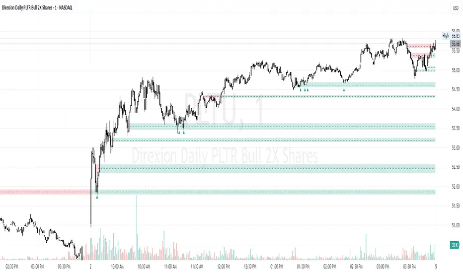
Bollinger Levels Table - Horizontal Support ZonesBollinger Levels Table - Horizontal Support Zones Indicator (with Customizable Options)
The "Bollinger Levels Table - Horizontal Support Zones" indicator is a comprehensive tool designed to help you identify potential support areas on your chart using moving averages and Bollinger Bands. The indicator displays an organized table of key price levels and draws horizontal lines on the chart, providing clear visibility of potential support zones.
What Does This Indicator Do?
This indicator aims to simplify support analysis by consolidating and displaying significant price levels derived from three different Bollinger Band settings: BB10, BB20, and BB50. It calculates both the Mid-line (Basis) and the Lower Band for each of these settings.
Furthermore, the indicator automatically arranges these levels from highest to lowest in an easy-to-read table, assigning a "Payment" label to each level. These "Payments" are simply labels to help you track the levels in descending order.
How Does This Indicator Work?
Bollinger Band Calculations: The indicator uses the standard Bollinger Band formula:
Mid-line (Basis): A Simple Moving Average (SMA) of the closing price over a specified period.
Standard Deviation (Dev): The standard deviation of the closing price over the same period, multiplied by a Multiplier.
Lower Band: The Mid-line minus the Standard Deviation.
These calculations are applied to three different periods: 10, 20, and 50, providing a variety of potential support levels based on different timeframes. You can adjust the values for these lengths (10, 20, 50) and the Multiplier through the indicator's settings.
Table Construction: A dynamic table is created on the chart (which can be positioned in the top or bottom right corner based on the current price's position). This table displays:
Indicator: The name of the Bollinger Band level (e.g., BB10 Mid, BB20 Lower).
Price: The exact price value of that level.
Payments: A label indicating the level's order in the table.
Level Ordering: All calculated levels are dynamically sorted from highest to lowest to present them in a logical order within the table.
Horizontal Line Plotting: Horizontal lines are drawn on the chart for each selected level, providing a visual representation of the potential support areas. These lines are colored black and have a consistent width for easy identification.
How to Use This Indicator:
This indicator is intended to provide potential entry points or accumulation zones for trades, especially for traders employing Dollar-Cost Averaging (DCA) strategies or building positions in stages. The levels displayed in the table and on the chart can represent potential support levels where one might consider initiating or adding to a position.
In the indicator's settings, you'll find important options:
Multiplier: Controls the width of the Bollinger Bands (default 2.0).
BB Lengths: Allows you to adjust the periods for the moving averages (default 20, 50, 10).
Visible Levels: This is the new feature! Here, you can select which levels you wish to see in the table and on the chart. Simply check or uncheck the boxes next to each level (BB10 Mid, BB10 Lower, and so on) to customize the indicator's display according to your strategy and needs.
Underlying Concepts:
This indicator is based on the principle that Bollinger Bands can act as dynamic support and resistance zones.
Mid-line (SMA): Often functions as a medium-term support or resistance.
Lower Band: Typically indicates that the price is relatively low and may find support, making it a potential area for buying or starting to build a position.
By combining different Bollinger Band timeframes (10, 20, 50), the indicator gives you a multi-timeframe perspective on support areas, helping you identify the most relevant levels for your strategy.
Note: While the indicator provides "Payments" for the levels, this is purely a sequential labeling within the table to assist your position-building strategy. There is no actual payment functionality associated with this indicator.
DECODE Moving Average ToolkitDECODE Moving Average Toolkit: Your All-in-One MA Analysis Powerhouse!
This versatile indicator is designed to be your go-to solution for analysing trends, identifying potential entry/exit points, and staying ahead of market movements using the power of Moving Averages (MAs).
Whether you're a seasoned trader or just starting out, the Decode MAT offers a comprehensive suite of features in a user-friendly package.
Key Features:
Multiple Moving Averages: Visualize up to 10 Moving Averages simultaneously on your chart.
Includes 5 Exponential Moving Averages (EMAs) and 5 Simple Moving Averages (SMAs).
Easily toggle the visibility of each MA and customize its length to suit your trading style and the asset you're analyzing.
Dynamic MA Ribbons: Gain a clearer perspective on trend direction and strength with 5 configurable MA Ribbons.
Each ribbon is formed between a corresponding EMA and SMA (e.g., EMA 20 / SMA 20).
The ribbon color changes to indicate bullish (e.g., green) or bearish (e.g., red) sentiment, providing an intuitive visual cue.
Toggle ribbon visibility with a single click.
Powerful Crossover Alerts: Never miss a potential trading opportunity with up to 5 customizable MA Crossover Alerts.
Define your own fast and slow MAs for each alert from any of the 10 available MAs.
Receive notifications directly through TradingView when your specified MAs cross over or cross under.
Optionally display visual symbols (e.g., triangles ▲▼) directly on your chart at the exact crossover points for quick identification.
Highly Customizable:
Adjust the source price (close, open, etc.) for all MA calculations.
Fine-tune the appearance (colors, line thickness) of every MA line, ribbon, and alert symbol to match your charting preferences.
User-Friendly Interface: All settings are neatly organized in the indicator's input menu, making configuration straightforward and intuitive.
How Can You Use the Decode MAT in Your Trading?
This toolkit is incredibly versatile and can be adapted to various trading strategies:
Trend Identification:
Use longer-term MAs (e.g., 50, 100, 200 period) to identify the prevailing market trend. When prices are consistently above these MAs, it suggests an uptrend, and vice-versa.
Observe the MA ribbons: A consistently green ribbon can indicate a strong uptrend, while a red ribbon can signal a downtrend. The widening or narrowing of the ribbon can also suggest changes in trend momentum.
Dynamic Support & Resistance:
Shorter-term MAs (e.g., 10, 20 period EMAs) can act as dynamic levels of support in an uptrend or resistance in a downtrend. Look for price pullbacks to these MAs as potential entry opportunities.
Crossover Signals (Entries & Exits):
Golden Cross / Death Cross: Configure alerts for classic crossover signals. For example, a 50-period MA crossing above a 200-period MA (Golden Cross) is often seen as a long-term bullish signal. Conversely, a 50-period MA crossing below a 200-period MA (Death Cross) can be a bearish signal.
Shorter-Term Signals: Use crossovers of shorter-term MAs (e.g., EMA 10 crossing EMA 20) for more frequent, shorter-term trading signals. A fast MA crossing above a slow MA can signal a buy, while a cross below can signal a sell.
Use the on-chart symbols for quick visual confirmation of these crossover events.
Confirmation Tool:
Combine the Decode MAT with other indicators (like RSI, MACD, or volume analysis) to confirm signals and increase the probability of successful trades. For instance, a bullish MA crossover combined with an oversold RSI reading could strengthen a buy signal.
Multi-Timeframe Analysis:
Apply the toolkit across different timeframes to get a broader market perspective. A long-term uptrend on the daily chart, confirmed by a short-term bullish crossover on the 1-hour chart, can provide a higher-confidence entry.
The DECODE Moving Average Toolkit empowers you to tailor your MA analysis precisely to your needs.
Ratings AlgoThe ratings algo is my discount version of the many paid-for algorithms put out by numerous different companies. A technical "rating" (by default between -10 and 10) is produced for each candle, telling the user when to buy, sell, or hold. I took 11 of my personal favorite indicators to develop a rating system. They are:
50/200 SMA crossover
10/20 SMA crossover
10/20 LSMA crossover
10/20 EMA crossover
"Arnold" a rate-of-change analysis of a smoothed LSMA
PVT and OBV momentum
MACD
RSI
DMI
Fisher Transform
The ratings system is very basic (a more complex, detailed version will be coming in the future!) where each indicator returns -1, 0, or 1, and the MAs and Oscillators are stratified with a user-defined weighting. The total calculation is based on the function:
maweight * (average of MA ratings) + oscillator weight * (average of osc ratings)
If the total value > user-defined threshold, the bar is teal, and if > 2.5 * threshold, is green, and vice versa for orange/red respectively. Purple is given if the total value is close to zero.
"Strong" signals are printed if the bar changes to either green or red and exits are printed if the bars change from green/red to any other color.
A table is also produced showing what each indicator is indicating, either "Buy" "Sell" or "Hold.
Reversal Bands are printed, intended to be used as areas where a trade might be exited if the market is sideways. If a Strong Buy signal is produced, it may be a good idea to enter the trade, and hold until the price enters the reversal bands, then hold until a candle closes outside the band for the first time.
This indicator truly shines in trending markets (like most indicators), but with very fast-acting exit signals and reversal zones, will facilitate minimal losses and possibly even profits in sideways markets.
