Golden Setup V1Golden Setup V1 is an overlay indicator that automates Tony Rago’s “Golden Setup” price-level framework. It divides the chart into fixed “blockSize” intervals (default 100 points) and plots a series of key horizontal levels within each block—levels at 00, 12, 26, 33, 50, 62, 77 and 88 offsets. These levels act as dynamic support and resistance grids that roll up or down as price moves between blocks.
Key Features
Customizable Offsets
Define eight offset levels corresponding to Rago’s Golden Setup:
00 (Round Number)
12 (Target 12)
26 (First “Golden” level)
33 (Target 33)
50 (Mid-block pivot)
62 (Target 62)
77 (Second “Golden” level)
88 (Target 88)
Multi-Block Coverage
Choose how many blocks above and below the current 100-point block you wish to display, so you always have levels drawn for the surrounding price range.
Golden-Only Filter
A handy toggle lets you show only the two “Golden” offsets (26 & 77), which many traders prioritize for high-probability bounce or breakout areas.
Dynamic Nearest-Level Label
Highlights the closest Golden Setup level (to the right edge of the chart) with a movable label, so you always know which level price is approaching.
Full Styling Control
Customize line colors, widths, block size, label fonts and opacity to suit your charting style.
How It Works
Block Calculation
On each bar, the indicator computes the “current block” by flooring (close / blockSize) and multiplying back by blockSize.
Level Offsets
It adds each of the eight user-defined offsets to that block base (and, if price has moved below the lowest offset, shifts the block down one interval).
Drawing
Each level is drawn as a horizontal line extending across the chart for as many blocks above/below as you select.
Nearest-Level Detection
Within the present block, it calculates which of the plotted levels is closest to price and displays that value on the right edge.
Usage Tips
Use the Golden-Only filter to declutter and focus solely on the 26 & 77 levels, which often act as strong intra-block pivot points.
Combine with volume or momentum indicators to confirm bounces at these levels.
Adjust blockSize (e.g. 50 or 200) if you wish to work in smaller or larger price increments.
⚠️ Disclaimer: This script is for educational and illustrative purposes only. Trading involves risk—always back-test and validate any strategy on a demo account before going live.
"摩根纳斯达克100基金风险大吗" için komut dosyalarını ara
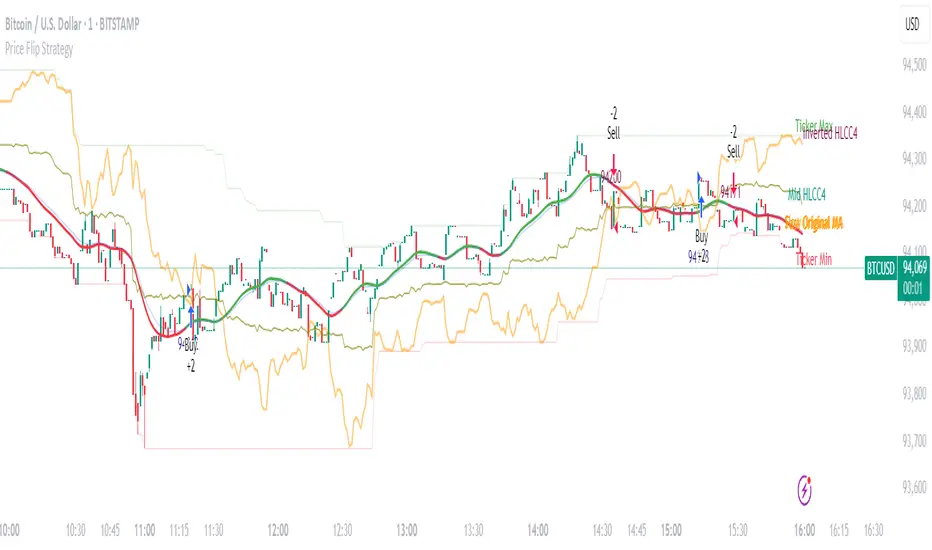
Price Flip StrategyPrice Flip Strategy with User-Defined Ticker Max/Max
This strategy leverages an inverted price calculation based on user-defined maximum and minimum price levels over customizable lookback periods. It generates buy and sell signals by comparing the previous bar's original price to the inverted price, within a specified date range. The script plots key metrics, including ticker max/min, original and inverted prices, moving averages, and HLCC4 averages, with customizable visibility toggles and labels for easy analysis.
Key Features:
Customizable Inputs: Set lookback periods for ticker max/min, moving average length, and date range for signal generation.
Inverted Price Logic: Calculates an inverted price using ticker max/min to identify trading opportunities.
Flexible Visualization: Toggle visibility for plots (e.g., ticker max/min, prices, moving averages, HLCC4 averages) and last-bar labels with user-defined colors and sizes.
Trading Signals: Generates buy signals when the previous original price exceeds the inverted price, and sell signals when it falls below, with alerts for real-time notifications.
Labeling: Displays values on the last bar for all plotted metrics, aiding in quick reference.
How to Use:
Add to Chart: Apply the script to a TradingView chart via the Pine Editor.
Configure Settings:
Date Range: Set the start and end dates to define the active trading period.
Ticker Levels: Adjust the lookback periods for calculating ticker max and min (e.g., 100 bars for max, 100 for min).
Moving Averages: Set the length for exponential moving averages (default: 20 bars).
Plots and Labels: Enable/disable specific plots (e.g., Inverted Price, Original HLCC4) and customize label colors/sizes for clarity.
Interpret Signals:
Buy Signal: Triggered when the previous close price is above the inverted price; marked with an upward label.
Sell Signal: Triggered when the previous close price is below the inverted price; marked with a downward label.
Set Alerts: Use the built-in alert conditions to receive notifications for buy/sell signals.
Analyze Plots: Review plotted lines (e.g., ticker max/min, HLCC4 averages) and last-bar labels to assess price behavior.
Tips:
Use in trending markets by enabling ticker max for uptrends or ticker min for downtrends, as indicated in tooltips.
Adjust the label offset to prevent overlapping text on the last bar.
Test the strategy on a demo account to optimize lookback periods and moving average settings for your asset.
Disclaimer: This script is for educational purposes and should be tested thoroughly before use in live trading. Past performance is not indicative of future results.
Machine Learning | Adaptive Trend Signals [Bitwardex]⚙️🧠Machine Learning | Adaptive Trend Signals
🔷Overview
Machine Learning | Adaptive Trend Signals is a Pine Script™ v6 indicator designed to visualize market trends and generate signals through a combination of volatility clustering, Gaussian smoothing, and adaptive trend calculations. Built as an overlay indicator, it integrates advanced techniques inspired by machine learning concepts, such as K-Means clustering, to adapt to changing market conditions. The script is highly customizable, includes a backtesting module, and supports alert conditions, making it suitable for traders exploring trend-based strategies and developers studying volatility-driven indicator design.
🔷Functionality
The indicator performs the following core functions:
• Volatility Clustering: Uses K-Means clustering to categorize market volatility into high, medium, and low states, adjusting trend sensitivity accordingly.
• Trend Calculation: Computes adaptive trend lines (SmartTrend) based on volatility-adjusted standard deviation, smoothed RSI, and ADX filters.
• Signal Generation: Identifies potential buy and sell points through trend line crossovers and directional confirmation.
• Backtesting Module: Tracks trade outcomes based on the SmartTrend3 value, displaying win rate and total trades.
• Visualization: Plots trend lines with gradient colors and optional signal markers (bullish 🐮 and bearish 🐻).
• Alerts: Provides configurable alerts for trend shifts and volatility state changes.
🔷Technical Methodology
Volatility Clustering with K-Means
The indicator employs a K-Means clustering algorithm to classify market volatility, measured via the Average True Range (ATR), into three distinct clusters:
• Data Collection: Gathers ATR values over a user-defined training period (default: 100 bars).
• Centroid Initialization: Sets initial centroids at the highest, lowest, and midpoint ATR values within the training period.
• Iterative Clustering: Assigns ATR data points to the nearest centroid, recalculates centroid means, and repeats until convergence.
• Dynamic Adjustment: Assigns a volatility state (high, medium, or low) based on the closest centroid, adjusting the trend factor (e.g., tighter for high volatility, wider for low volatility).
This approach allows the indicator to adapt its sensitivity to varying market conditions, providing a data-driven foundation for trend calculations.
🔷Gaussian Smoothing
To enhance signal clarity and reduce noise, the indicator applies Gaussian kernel smoothing to:
• RSI: Smooths the Relative Strength Index (calculated from OHLC4) to filter short-term fluctuations.
• SmartTrend: Smooths the primary trend line for a more stable output.
The Gaussian kernel uses a sigma value derived from the user-defined smoothing length, ensuring mathematically consistent noise reduction.
🔷SmartTrend Calculation
The pineSmartTrend function is the core of the indicator, producing three trend lines:
• SmartTrend: The primary trend line, calculated using a volatility-adjusted standard deviation, smoothed RSI, and ADX conditions.
• SmartTrend2: A secondary trend line with a wider factor (base factor * 1.382) for signal confirmation.
SmartTrend3: The average of SmartTrend and SmartTrend2, used for plotting and backtesting.
Key components of the calculation include:
• Dynamic Standard Deviation: Scales based on ATR relative to its 50-period smoothed average, with multipliers (1.0 to 1.4) applied according to volatility thresholds.
• RSI and ADX Filters: Requires RSI > 50 for bullish trends or < 50 for bearish trends, alongside ADX > 15 and rising to confirm trend strength.
Volatility-Adjusted Bands: Constructs upper and lower bands around price action, adjusted by the volatility cluster’s dynamic factor.
🔷Signal Generation
The generate_signals function generates signals as follows:
• Buy Signal: Triggered when SmartTrend crosses above SmartTrend2 and the price is above SmartTrend, with directional confirmation.
• Sell Signal: Triggered when SmartTrend crosses below SmartTrend2 and the price is below SmartTrend, with directional confirmation.
Directional Logic: Tracks trend direction to filter out conflicting signals, ensuring alignment with the broader market context.
Signals are visualized as small circles with bullish (🐮) or bearish (🐻) emojis, with an option to toggle visibility.
🔷Backtesting
The get_backtest function evaluates signal outcomes using the SmartTrend3 value (rather than closing prices) to align with the trend-based methodology.
It tracks:
• Total Trades: Counts completed long and short trades.
• Win Rate: Calculates the percentage of trades where SmartTrend3 moves favorably (higher for longs, lower for shorts).
Position Management: Closes opposite positions before opening new ones, simulating a single-position trading system.
Results are displayed in a table at the top-right of the chart, showing win rate and total trades. Note that backtest results reflect the indicator’s internal logic and should not be interpreted as predictive of real-world performance.
🔷Visualization and Alerts
• Trend Lines: SmartTrend3 is plotted with gradient colors reflecting trend direction and volatility cluster, accompanied by a secondary line for visual clarity.
• Signal Markers: Optional buy/sell signals are plotted as small circles with customizable colors.
• Alerts: Supports alerts for:
• Bullish and bearish trend shifts (confirmed on bar close).
Transitions to high, medium, or low volatility states.
🔷Input Parameters
• ATR Length (default: 14): Period for ATR calculation, used in volatility clustering.
• Period (default: 21): Common period for RSI, ADX, and standard deviation calculations.
• Base SmartTrend Factor (default: 2.0): Base multiplier for volatility-adjusted bands.
• SmartTrend Smoothing Length (default: 10): Length for Gaussian smoothing of the trend line.
• Show Buy/Sell Signals? (default: true): Enables/disables signal markers.
• Bullish/Bearish Color: Customizable colors for trend lines and signals.
🔷Usage Instructions
• Apply to Chart: Add the indicator to any TradingView chart.
• Configure Inputs: Adjust parameters to align with your trading style or market conditions (e.g., shorter ATR length for faster markets).
• Interpret Output:
• Trend Lines: Use SmartTrend3’s direction and color to gauge market bias.
• Signals: Monitor bullish (🐮) and bearish (🐻) markers for potential entry/exit points.
• Backtest Table: Review win rate and total trades to understand the indicator’s behavior in historical data.
• Set Alerts: Configure alerts for trend shifts or volatility changes to support manual or automated trading workflows.
• Combine with Analysis: Use the indicator alongside other tools or market context, as it is designed to complement, not replace, comprehensive analysis.
🔷Technical Notes
• Data Requirements: Requires at least 100 bars for accurate volatility clustering. Ensure sufficient historical data is loaded.
• Market Suitability: The indicator is designed for trend detection and may perform differently in ranging or volatile markets due to its reliance on RSI and ADX filters.
• Backtesting Scope: The backtest module uses SmartTrend3 values, which may differ from price-based outcomes. Results are for informational purposes only.
• Computational Intensity: The K-Means clustering and Gaussian smoothing may increase processing time on lower timeframes or with large datasets.
🔷For Developers
The script is modular, well-commented, encouraging reuse and modification with proper attribution.
Key functions include:
• gaussianSmooth: Applies Gaussian kernel smoothing to any data series.
• pineSmartTrend: Computes adaptive trend lines with volatility and momentum filters.
• getDynamicFactor: Adjusts trend sensitivity based on volatility clusters.
• get_backtest: Evaluates signal performance using SmartTrend3.
Developers can extend these functions for custom indicators or strategies, leveraging the volatility clustering and smoothing methodologies. The K-Means implementation is particularly useful for adaptive volatility analysis.
🔷Limitations
• The indicator is not predictive and should be used as part of a broader trading strategy.
• Performance varies by market, timeframe, and parameter settings, requiring user experimentation.
• Backtest results are based on historical data and internal logic, not real-world trading conditions.
• Volatility clustering assumes sufficient historical data; incomplete data may affect accuracy.
🔷Acknowledgments
Developed by Bitwardex, inspired by machine learning concepts and adaptive trading methodologies. Community feedback is welcome via TradingView’s platform.
🔷 Risk Disclaimer
Trading involves significant risks, and most traders may incur losses. Bitwardex AI Algo is provided for informational and educational purposes only and does not constitute financial advice or a recommendation to buy or sell any financial instrument . The signals, metrics, and features are tools for analysis and do not guarantee profits or specific outcomes. Past performance is not indicative of future results. Always conduct your own due diligence and consult a financial advisor before making trading decisions.

Aggregate PDH High Break Alert**Aggregate PDH High Break Alert**
**Overview**
The “Aggregate PDH High Break Alert” is a lightweight Pine Script v6 indicator designed to instantly notify you when today’s price breaks above any prior-day high in a user-defined lookback window. Instead of manually scanning dozens of daily highs, this script automatically loops through the last _N_ days (up to 100) and fires a single-bar alert the moment price eclipses a specific day’s high.
**Key Features**
- **Dynamic Lookback**: Choose any lookback period from 1 to 100 days via a single `High-Break Lookback` input.
- **Single Security Call**: Efficiently retrieves the entire daily-high series in one call to avoid TradingView’s 40-call security limit.
- **Automatic Looping**: Internally loops through each prior-day high, so there’s no need to manually code dozens of lines.
- **Custom Alerts**: Generates a clear, formatted alert message—e.g. “Crossed high from 7 day(s) ago”—for each breakout.
- **Lightweight & Maintainable**: Compact codebase (<15 lines) makes tweaking and debugging a breeze.
**Inputs**
- **High-Break Lookback (days)**: Number of past days to monitor for high breaks. Valid range: 1–100.
**How to Use**
1. **Add to Chart**: Open TradingView, click “Indicators,” then “Create,” and paste in the code.
2. **Configure Lookback**: In the script’s settings, set your desired lookback window (e.g., 20 for the past 20 days).
3. **Enable Alerts**: Right-click the indicator’s name on your chart, select “Add Alert on Aggregate PDH High Break Alert,” and choose “Once per bar close.”
4. **Receive Notifications**: Whenever price crosses above any of the specified prior-day highs, you’ll get an on-screen and/or mobile push alert with the exact number of days ago.
**Use Cases**
- **Trend Confirmation**: Confirm fresh bullish momentum when today’s high outpaces any of the last _N_ days.
- **Breakout Trading**: Automate entries off multi-day highs without manual chart scanning.
- **System Integration**: Integrate with alerts to trigger orders in third-party bots or webhook receivers.
**Disclaimer**
Breakouts alone do not guarantee sustained moves. Combine with your preferred risk management, volume filters, and other indicators for higher-probability setups. Use on markets and timeframes where daily breakout behavior aligns with your strategy.

CyberCandle SwiftEdgeCyberCandle SwiftEdge
Overview
CyberCandle SwiftEdge is a cutting-edge, AI-inspired trading indicator designed for traders seeking precision and clarity in trend-following and swing trading. Powered by SwiftEdge, it combines Heikin Ashi candles, a gradient-colored Exponential Moving Average (EMA), and a Relative Strength Index (RSI) to deliver clear buy and sell signals. Featuring glowing visuals, dynamic signal icons, and a customizable RSI dashboard in the top-right corner, this script offers a futuristic interface for identifying high-probability trade setups on various timeframes (e.g., 1H, 4H).
What It Does
CyberCandle SwiftEdge integrates three powerful components to generate actionable trading signals:
Heikin Ashi Candles: Smooths price action to highlight trends, reducing market noise and making reversals easier to spot.
Gradient EMA: A 100-period EMA with dynamic color transitions (blue/cyan for uptrends, red/pink for downtrends) to confirm market direction.
RSI Dashboard: A neon-lit display showing RSI levels, indicating overbought (>70), oversold (<30), or neutral (30-70) conditions.
Buy and sell signals are marked with prominent, glowing icons (triangles and arrows) based on trend direction, momentum, and specific Heikin Ashi patterns. The script’s customizable parameters allow traders to tailor the strategy to their preferences, balancing signal frequency and precision.
How It Works
The strategy leverages the synergy of Heikin Ashi, EMA, and RSI to filter trades and highlight opportunities:
Trend Direction: The price must be above the EMA for buy signals (bullish trend) or below for sell signals (bearish trend). The EMA’s gradient color shifts based on its slope, visually reinforcing trend strength.
Momentum Confirmation: RSI must exceed a user-defined threshold (default: 50) for buy signals or fall below it for sell signals, ensuring momentum supports the trade.
Candle Patterns: Buy signals require a green Heikin Ashi candle (close > open), with the two prior candles having minimal upper wicks (≤5% of candle body) and being red (indicating a retracement). Sell signals require a red candle, minimal lower wicks, and two prior green candles.
RSI Dashboard: Positioned in the top-right corner, it features a glowing circle (red for overbought, green for oversold, blue for neutral), the current RSI value, and a status indicator (triangle for extremes, square for neutral). This provides instant momentum insights without cluttering the chart.
By combining Heikin Ashi’s trend clarity, EMA’s directional filter, and RSI’s momentum validation, CyberCandle SwiftEdge minimizes false signals and highlights trades with strong potential. Its vibrant, AI-like visuals make it easy to interpret at a glance.
How to Use It
Add to Chart: In TradingView, search for "CyberCandle SwiftEdge" and add it to your chart. Set the chart to Heikin Ashi candles for optimal compatibility.
Interpret Signals:
Buy Signal: Large green triangles and arrows appear below candles when the price is above the EMA, RSI is above the buy threshold (default: 50), and conditions for a bullish retracement are met. Consider entering a long position with a 1:2 risk/reward ratio.
Sell Signal: Large red triangles and arrows appear above candles when the price is below the EMA, RSI is below the sell threshold (default: 50), and conditions for a bearish retracement are met. Consider entering a short position.
RSI Dashboard: Monitor the top-right dashboard. A red circle (RSI > 70) suggests caution for buys, a green circle (RSI < 30) indicates potential buying opportunities, and a blue circle (RSI 30-70) signals neutrality.
Customize Parameters: Open the indicator’s settings to adjust:
EMA Length (default: 100): Increase (e.g., 200) for longer-term trends or decrease (e.g., 50) for shorter-term sensitivity.
RSI Length (default: 14): Adjust for more (e.g., 7) or less (e.g., 21) responsive momentum signals.
RSI Buy/Sell Thresholds (default: 50): Set higher (e.g., 55) for buys or lower (e.g., 45) for sells to require stronger momentum.
Wick Tolerance (default: 0.05): Increase (e.g., 0.1) to allow larger wicks, generating more signals, or decrease (e.g., 0.02) for stricter conditions.
Require Retracement (default: true): Disable to remove the two-candle retracement requirement, increasing signal frequency.
Trading: Use signals in conjunction with the RSI dashboard and market context. For example, avoid buy signals if the RSI dashboard is red (overbought). Always apply proper risk management, such as setting stop-losses based on recent lows/highs.
What Makes It Original
CyberCandle SwiftEdge stands out due to its futuristic, AI-inspired visual design and user-friendly customization:
Neon Aesthetics: Glowing Heikin Ashi candles, gradient EMA, and dynamic signal icons (triangles and arrows) with RSI-driven transparency create a high-tech, immersive experience.
RSI Dashboard: A compact, top-right display with a neon circle, RSI value, and adaptive status indicator (triangle/square) provides instant momentum insights without cluttering the chart.
Customizability: Users can fine-tune EMA length, RSI parameters, wick tolerance, and retracement requirements via TradingView’s settings, balancing signal frequency and precision.
Integrated Approach: The synergy of Heikin Ashi’s trend clarity, EMA’s directional strength, and RSI’s momentum validation offers a cohesive strategy that reduces false signals.
Why This Combination?
The script combines Heikin Ashi, EMA, and RSI for a complementary effect:
Heikin Ashi smooths price fluctuations, making it ideal for identifying sustained trends and retracements, which are critical for the strategy’s signal logic.
EMA provides a reliable trend filter, ensuring signals align with the broader market direction. Its gradient color enhances visual trend recognition.
RSI adds momentum context, confirming that signals occur during favorable conditions (e.g., RSI > 50 for buys). The dashboard makes RSI intuitive, even for non-technical users.
Together, these components create a balanced system that captures trend reversals after retracements, validated by momentum, with a visually engaging interface that simplifies decision-making.
Tips
Best used on volatile assets (e.g., BTC/USD, EUR/USD) and higher timeframes (1H, 4H) for clearer trends.
Experiment with parameters in the settings to match your trading style (e.g., increase wick tolerance for more signals).
Combine with other analysis (e.g., support/resistance) for higher-confidence trades.
Note
This indicator is for informational purposes and does not guarantee profits. Always backtest and use proper risk management before trading.
Clenow MomentumClenow Momentum Method
The Clenow Momentum Method, developed by Andreas Clenow, is a systematic, quantitative trading strategy focused on capturing medium- to long-term price trends in financial markets. Popularized through Clenow’s book, Stocks on the Move: Beating the Market with Hedge Fund Momentum Strategies, the method leverages momentum—an empirically observed phenomenon where assets that have performed well in the recent past tend to continue performing well in the near future.
Theoretical Foundation
Momentum investing is grounded in behavioral finance and market inefficiencies. Investors often exhibit herding behavior, underreact to new information, or chase trends, causing prices to trend beyond fundamental values. Clenow’s method builds on academic research, such as Jegadeesh and Titman (1993), which demonstrated that stocks with high returns over 3–12 months outperform those with low returns over similar periods.
Clenow’s approach specifically uses **annualized momentum**, calculated as the rate of return over a lookback period (typically 90 days), annualized to reflect a yearly percentage. The formula is:
Momentum=(((Close N periods agoCurrent Close)^N252)−1)×100
- Current Close: The most recent closing price.
- Close N periods ago: The closing price N periods back (e.g., 90 days).
- N: Lookback period (commonly 90 days).
- 252: Approximate trading days in a year for annualization.
This metric ranks stocks by their momentum, prioritizing those with the strongest upward trends. Clenow’s method also incorporates risk management, diversification, and volatility adjustments to enhance robustness.
Methodology
The Clenow Momentum Method involves the following steps:
1. Universe Selection:
- A broad universe of liquid stocks is chosen, often from major indices (e.g., S&P 500, Nasdaq 100) or global exchanges.
- Filters should exclude illiquid stocks (e.g., low average daily volume) or those with extreme volatility.
2. Momentum Calculation:
- Stocks are ranked based on their annualized momentum over a lookback period (typically 90 days, though 60–120 days can be common tests).
- The top-ranked stocks (e.g., top 10–20%) are selected for the portfolio.
3. Volatility Adjustment (Optional):
- Clenow sometimes adjusts momentum scores by volatility (e.g., dividing by the standard deviation of returns) to favor stocks with smoother trends.
- This reduces exposure to erratic price movements.
4. Portfolio Construction:
- A diversified portfolio of 10–25 stocks is constructed, with equal or volatility-weighted allocations.
- Position sizes are often adjusted based on risk (e.g., 1% of capital per position).
5. Rebalancing:
- The portfolio is rebalanced periodically (e.g., weekly or monthly) to maintain exposure to high-momentum stocks.
- Stocks falling below a momentum threshold are replaced with higher-ranked candidates.
6. Risk Management:
- Stop-losses or trailing stops may be applied to limit downside risk.
- Diversification across sectors reduces concentration risk.
Implementation in TradingView
Key features include:
- Customizable Lookback: Users can adjust the lookback period in pinescript (e.g., 90 days) to align with Clenow’s methodology.
- Visual Cues: Background colors (green for positive, red for negative momentum) and a zero line help identify trend strength.
- Integration with Screeners: TradingView’s stock screener can filter high-momentum stocks, which can then be analyzed with the custom indicator.
Strengths
1. Simplicity: The method is straightforward, relying on a single metric (momentum) that’s easy to calculate and interpret.
2. Empirical Support: Backed by decades of academic research and real-world hedge fund performance.
3. Adaptability: Applicable to stocks, ETFs, or other asset classes, with flexible lookback periods.
4. Risk Management: Diversification and periodic rebalancing reduce idiosyncratic risk.
5. TradingView Integration: Pine Script implementation enables real-time visualization, enhancing decision-making for stocks like NVDA or SPY.
Limitations
1. Mean Reversion Risk: Momentum can reverse sharply in bear markets or during sector rotations, leading to drawdowns.
2. Transaction Costs: Frequent rebalancing increases trading costs, especially for retail traders with high commissions. This is not as prevalent with commission free trading becoming more available.
3. Overfitting Risk: Over-optimizing lookback periods or filters can reduce out-of-sample performance.
4. Market Conditions: Underperforms in low-momentum or highly volatile markets.
Practical Applications
The Clenow Momentum Method is ideal for:
Retail Traders: Use TradingView’s screener to identify high-momentum stocks, then apply the Pine Script indicator to confirm trends.
Portfolio Managers: Build diversified momentum portfolios, rebalancing monthly to capture trends.
Swing Traders: Combine with volume filters to target short-term breakouts in high-momentum stocks.
Cross-Platform Workflow: Integrate with Python scanners to rank stocks, then visualize on TradingView for trade execution.
Comparison to Other Strategies
Vs. Minervini’s VCP: Clenow’s method is purely quantitative, while Minervini’s Volatility Contraction Pattern (your April 11, 2025 query) combines momentum with chart patterns. Clenow is more systematic but less discretionary.
Vs. Mean Reversion: Momentum bets on trend continuation, unlike mean reversion strategies that target oversold conditions.
Vs. Value Investing: Momentum outperforms in bull markets but may lag value strategies in recovery phases.
Conclusion
The Clenow Momentum Method is a robust, evidence-based strategy that capitalizes on price trends while managing risk through diversification and rebalancing. Its simplicity and adaptability make it accessible to retail traders, especially when implemented on platforms like TradingView with custom Pine Script indicators. Traders must be mindful of transaction costs, mean reversion risks, and market conditions. By combining Clenow’s momentum with volume filters and alerts, you can optimize its application for swing or position trading.
Highest/Lowest Range in TimeframeThis script helps traders visually identify the highest high and lowest low within a customizable range of recent bars.
🔍 Key Features
Scans the last 100 to 1000 bars (user-defined)
Automatically detects:
The highest wick (high) and lowest wick (low)
Draws dotted green horizontal lines at both levels
Shows a label indicating the percentage range between high and low
Displays real-time high and low price labels directly on the chart
⚙️ Use Cases
Quickly spot price extremes over your desired time window
Visually measure market range and volatility
Identify breakout potential or reversal zones
✅ How to Use
Add the script to your chart.
Set the “Bars to Scan” input to your desired lookback period (between 100–1000).
Use the displayed lines and labels to identify key high/low price levels and range metrics.

Log-Normal Price ForecastLog-Normal Price Forecast
This Pine Script creates a log-normal forecast model of future price movements on a TradingView chart, based on historical log returns. It plots expected price trajectories and bands representing different levels of statistical deviation.
Parameters
Model Length – Number of bars used to calculate average and standard deviation of log returns (default: 100).
Forecast Length – Number of bars into the future for which the forecast is projected (default: 100, max: 500).
Volatility SMA Length – The smoothing length for the standard deviation (default: 20).
Confidence Intervals – Confidence intervals for price bands (default: 95%, 99%, 99.9%).

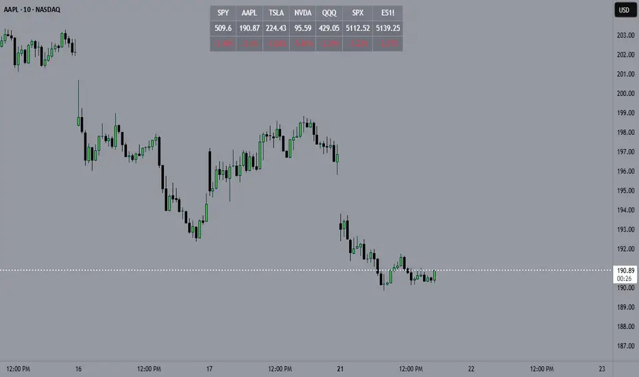
Horizontal Price TableOverview:
This script displays a dynamic price table on your chart, showing real-time prices and daily percentage changes for up to 7 user-defined tickers. You can customize both which tickers are shown and how many are visible, all through the settings panel.
How it works (Step-by-Step):
User-Defined Tickers:
The script provides input fields for up to 7 tickers using input.symbol(). You can track stocks, indexes, ETFs, crypto, or futures — anything supported by TradingView.
Choose How Many to Display:
An additional dropdown lets you choose how many of the 7 tickers to actually display (between 1 and 7). This gives you control over screen space and focus.
Market Data Fetching:
For each displayed ticker, the script fetches:
The current day’s closing price (close)
The previous day’s closing price (close )
This data is pulled using request.security() on the daily timeframe (1D).
% Change Calculation:
The script calculates the daily percentage change using:
(Current Price−Previous Close)/Previous Close×100(Current Price−Previous Close)/Previous Close×100
Cleaned Ticker Names:
Ticker symbols often include an exchange prefix like NASDAQ:AAPL. The script automatically removes anything before the colon (:), so only the clean symbol (e.g., AAPL) is shown in the table.
Table Display:
A visual table appears at the top-center of your chart, showing:
Row 1: Ticker symbol (cleaned)
Row 2: Current price (rounded to 2 decimals)
Row 3: Daily % change (green for gains, red for losses)
Customization:
You can choose the background color of the table.
Ticker names appear in white text with a gray background.
% change is color-coded: green for positive, red for negative.
Why Use This Script?
Track multiple tickers at once without leaving your chart.
Clean, customizable layout.
Useful for monitoring watchlists, portfolios, or related markets.
Tips:
Combine this with your favorite indicators for a personalized dashboard.
Works great on any chart or timeframe.
Ensure the tickers entered are valid on TradingView (e.g., SPY, BTCUSD, NQ1!, etc.).
RSI+Stoch Band Oscillator📈 RSI + Stochastic Band Oscillator
Overview:
The RSI + Stochastic Band Oscillator is a technical indicator that combines the strengths of both the Relative Strength Index (RSI) and the Stochastic Oscillator. Instead of using static thresholds, this indicator dynamically constructs upper and lower bands based on the RSI and Stochastic overbought/oversold zones. It then measures the relative position of the current price within this adaptive range, effectively producing a normalized oscillator.
Key Components:
RSI-Based Dynamic Bands:
Using RSI values and exponential moving averages of price changes, upper and lower dynamic bands are constructed.
These bands adjust based on overbought and oversold levels, offering a more responsive framework than fixed RSI thresholds.
Stochastic-Based Dynamic Bands:
Similarly, Stochastic %K and %D values are used to construct dynamic bands.
These adapt to overbought and oversold levels by recalculating potential high/low values within the lookback window.
Oscillator Calculation:
The oscillator (osc) is computed as the relative position of the current close within the combined upper and lower bands of both RSI and Stochastic.
This value is normalized between 0 and 100, allowing clear identification of extreme conditions.
Visual Features:
The oscillator is plotted as a line between 0 and 100.
Color-filled areas highlight when the oscillator enters extreme zones:
Above 100 with falling momentum: Red zone (potential reversal).
Below 0 with rising momentum: Green zone (potential reversal).
Additional trend conditions (falling/rising RSI, %K, and %D) are used to strengthen reversal signals by confirming momentum shifts.

Weighted Ichimoku StrategyLSE:HSBA
The Ichimoku Kinko Hyo indicator is a comprehensive tool that combines multiple signals to identify market trends and potential buying/selling opportunities. My weighted variant of this strategy attempts to assign specific weights to each signal, allowing for a more nuanced and customizable approach to trend identification. The intent is to try and make a more informed trading decision based on the cumulative strength of various signals.
I've tried not to make it a mishmash of this and that + MACD + RSI and on and on; most people have their preferred indicator that focuses on just that that they can use in conjunction.
The signals used can be grouped into two groups the 'Core Ichimoku Signals' & the 'Additional Signals' (at the end you will find the signals and their assigned weights followed by the thresholds where they align).
The Core Ichimoku Signals are the primary signals used in Ichimoku analysis, including Kumo Breakout, Chikou Cross, Kijun Cross, Tenkan Cross, and Kumo Twist.
While the Additional Signals provide further insights and confirmations, such as Kijun Confirmation, Tenkan-Kijun Above Cloud, Chikou Above Cloud, Price-Kijun Cross, Chikou Span Signal, and Price Positioning.
Entries are triggered when the cumulative weight of bullish signals exceeds a specified buy threshold, indicating a strong uptrend or potential trend reversal.
Exits are initiated when the cumulative weight of bearish signals surpasses a specified sell threshold, or when additional conditions such as consolidation patterns or ATR-based targets are met.
There are various exit types that you can choose between, which can be used separately or in conjunction with one another. As an example you might want to exit on a different condition during consolidation periods than during other periods or just use ATR with some other backstop.
They are listed in evaluation order i.e. ATR trumps all, Consolidation exit trumps the regular Kumo sell and so on:
**ATR Sell**: Exits trades based on ATR-based profit targets and stop-losses.
**Consolidation Exit**: Exits trades during consolidation periods to reduce drawdown.
**Sell Below Kumo**: Exits trades when the price is below the Kumo, indicating a potential downtrend.
**Sell Threshold**: Exits trades when the cumulative weight of bearish signals surpasses a specified sell threshold.
There are various 'filters' which are really behavior modifiers:
**Kumo Breakout Filter**: Requires price to close above the Kumo for buy signals (essentially a entry delay).
**Whipsaw Filter**: Ensures trend strength over specified days to reduce false signals.
**Buy Cooldown**: Prevents new entries until half the Kijun period passes after an exit (prevents flapping).
**Chikou Filter**: Delays exits unless the previous close is below the Chikou Span.
**Consolidation Trend Filter**: Prevents consolidation exits if the trend is bullish (rare, but happens).
Then there are some debugging options. Ichimoku periods have some presets (personally I like 8/22/44/22) but are freely configurable, preset to the traditional values for purists.
The list of signals and most thresholds follow, play around with them. Thats all.
Cheers,
**Core Ichimoku Signals**
**Kumo Breakout**
- 30 (Bullish) / -30 (Bearish)
- Indicates a strong trend when the price breaks above (bullish) or below (bearish) the Kumo (cloud). This signal suggests a significant shift in market sentiment.
**Chikou Cross**
- 20 (Bullish) / -20 (Bearish)
- Shows the relationship between the Chikou Span (lagging span) and the current price. A bullish signal occurs when the Chikou Span is above the price, indicating a potential uptrend. Conversely, a bearish signal occurs when the Chikou Span is below the price, suggesting a downtrend.
**Kijun Cross**
- 15 (Bullish) / -15 (Bearish)
- Signals trend changes when the Tenkan-sen (conversion line) crosses above (bullish) or below (bearish) the Kijun-sen (base line). This crossover is often used to identify potential trend reversals.
**Tenkan Cross**
- 10 (Bullish) / -10 (Bearish)
- Indicates short-term trend changes when the price crosses above (bullish) or below (bearish) the Tenkan-sen. This signal helps identify minor trend shifts within the broader trend.
**Kumo Twist**
- 5 (Bullish) / -5 (Bearish)
- Shows changes in the Kumo's direction, indicating potential trend shifts. A bullish Kumo Twist occurs when Senkou Span A crosses above Senkou Span B, and a bearish twist occurs when Senkou Span A crosses below Senkou Span B.
**Additional Signals**
**Kijun Confirmation**
- 8 (Bullish) / -8 (Bearish)
- Confirms the trend based on the price's position relative to the Kijun-sen. A bullish signal occurs when the price is above the Kijun-sen, and a bearish signal occurs when the price is below it.
**Tenkan-Kijun Above Cloud**
- 5 (Bullish) / -5 (Bearish)
- Indicates a strong bullish trend when both the Tenkan-sen and Kijun-sen are above the Kumo. Conversely, a bearish signal occurs when both lines are below the Kumo.
**Chikou Above Cloud**
- 5 (Bullish) / -5 (Bearish)
- Shows the Chikou Span's position relative to the Kumo, indicating trend strength. A bullish signal occurs when the Chikou Span is above the Kumo, and a bearish signal occurs when it is below.
**Price-Kijun Cross**
- 2 (Bullish) / -2 (Bearish)
- Signals short-term trend changes when the price crosses above (bullish) or below (bearish) the Kijun-sen. This signal is similar to the Kijun Cross but focuses on the price's direct interaction with the Kijun-sen.
**Chikou Span Signal**
- 10 (Bullish) / -10 (Bearish)
- Indicates the trend based on the Chikou Span's position relative to past price highs and lows. A bullish signal occurs when the Chikou Span is above the highest high of the past period, and a bearish signal occurs when it is below the lowest low.
**Price Positioning**
- 10 (Bullish) / -10 (Bearish)
- Shows indecision when the price is between the Tenkan-sen and Kijun-sen, indicating a potential consolidation phase. A bullish signal occurs when the price is above both lines, and a bearish signal occurs when the price is below both lines.
**Confidence Level**: Highly Sensitive
- **Buy Threshold**: 50
- **Sell Threshold**: -50
- **Notes / Significance**: ~2–3 signals, very early trend detection. High sensitivity, may capture noise and false signals.
**Confidence Level**: Entry-Level
- **Buy Threshold**: 58
- **Sell Threshold**: -58
- **Notes / Significance**: ~3–4 signals, often Chikou Cross or Kumo Breakout. Very sensitive, risks noise (e.g., false buys in choppy markets).
**Confidence Level**: Entry-Level
- **Buy Threshold**: 60
- **Sell Threshold**: -60
- **Notes / Significance**: ~3–4 signals, Kumo Breakout or Chikou Cross anchors. Entry point for early trends.
**Confidence Level**: Moderate
- **Buy Threshold**: 65
- **Sell Threshold**: -65
- **Notes / Significance**: ~4–5 signals, balances sensitivity and reliability. Suitable for moderate risk tolerance.
**Confidence Level**: Conservative
- **Buy Threshold**: 70
- **Sell Threshold**: -70
- **Notes / Significance**: ~4–5 signals, emphasizes stronger confirmations. Reduces false signals but may miss some opportunities.
**Confidence Level**: Very Conservative
- **Buy Threshold**: 75
- **Sell Threshold**: -75
- **Notes / Significance**: ~5–6 signals, prioritizes high confidence. Minimizes risk but may enter trades late.
**Confidence Level**: High Confidence
- **Buy Threshold**: 80
- **Sell Threshold**: -80
- **Notes / Significance**: ~6–7 signals, very strong confirmations needed. Suitable for cautious traders.
**Confidence Level**: Very High Confidence
- **Buy Threshold**: 85
- **Sell Threshold**: -85
- **Notes / Significance**: ~7–8 signals, extremely high confidence required. Minimizes false signals significantly.
**Confidence Level**: Maximum Confidence
- **Buy Threshold**: 90
- **Sell Threshold**: -90
- **Notes / Significance**: ~8–9 signals, maximum confidence level. Ensures trades are highly reliable but may result in fewer trades.
**Confidence Level**: Ultra Conservative
- **Buy Threshold**: 100
- **Sell Threshold**: -100
- **Notes / Significance**: ~9–10 signals, ultra-high confidence. Trades are extremely reliable but opportunities are rare.
**Confidence Level**: Extreme Confidence
- **Buy Threshold**: 110
- **Sell Threshold**: -110
- **Notes / Significance**: All signals align, extreme confidence. Trades are almost certain but very few opportunities.
Volume and Volatility Ratio Indicator-WODI该指标名为“交易量与波动率比例指标-WODI”,主要基于交易量和价格波动率构造一个复合指数,帮助识别市场内可能存在的异常或转折信号。具体实现如下:
用户自定义参数
用户可以设置交易量均线长度(vol_length)、指数的短期与长期均线长度(index_short_length、index_long_length)、均线敏感度(index_magnification)、阈值放大因子(index_threshold_magnification)以及检测K线形态的区间(lookback_bars)。这些参数为后续计算提供了灵活性,允许用户根据不同市场环境自定义指标的敏感度和响应速度。
交易量均线与百分比计算
首先通过 ta.sma 计算指定长度的交易量简单均线(vol_ma)。
接下来,将当前交易量与均线进行比较,计算出当前交易量占均线的百分比(vol_percent),这反映了短期内交易量的相对活跃程度。
波动率的衡量
使用当前K线的最高价和最低价计算振幅,再除以收盘价乘以100得到波动率(volatility),从而反映市场价格波动的幅度。
构建交易量/波动率指数
将交易量百分比与波动率相乘,形成了“交易量/波动率指数”(volatility_index)。该指数能够同时反映市场的交易活跃度和价格波动性,两者的联合作用帮助捕捉市场的“热度”。
计算指标均线与阈值
对交易量/波动率指数分别计算短期均线(index_short_ma)和长期均线(index_long_ma),并通过乘以一个敏感度参数(index_magnification)进行调整。
同时,依据长期均线计算一个阈值(index_threshold),起到过滤噪音的作用。当指数突破该阈值时,可能预示着市场的重要变化。
K线形态与反转模式检测
通过遍历最近几根K线(由lookback_bars控制),指标会检测是否符合一系列预定条件(涉及交易量、价格振幅、K线形态等),以判断是否存在反转模式。若符合条件,则标记为反转模式,从而为潜在的转折点提供提示。
图表展示
最终在独立窗口中绘制多个元素:
指数短均线与长均线:经过敏感度调整后显示,用于分析指数趋势。
交易量/波动率指数:采用阶梯线风格绘制,直观展示指数变化。
阈值线:作为参考水平,便于判断指数是否突破常规范围。
交易量柱状图:当当前交易量高于均线时,通过不同颜色显示;当检测到反转模式时,颜色会进一步强化,帮助用户迅速识别潜在信号。
English Description
This indicator, titled “Volume and Volatility Ratio Indicator - WODI”, is designed to construct a composite index based on trading volume and price volatility, aiding in the identification of abnormal market conditions or potential reversal signals. Its functionality is broken down as follows:
User-Defined Parameters
The indicator allows users to set parameters such as the moving average length for volume (vol_length), the short and long moving average lengths for the index (index_short_length and index_long_length), a sensitivity multiplier (index_magnification), a threshold magnification factor (index_threshold_magnification), and the number of bars for pattern detection (lookback_bars). These parameters provide flexibility to adjust the sensitivity and responsiveness of the indicator based on different market conditions.
Volume Moving Average and Percentage Calculation
A simple moving average (SMA) of volume is computed over the specified length (vol_ma) using the ta.sma function.
The current volume is then compared to its moving average to calculate the volume percentage (vol_percent), reflecting the relative trading intensity in the short term.
Measuring Volatility
Volatility is calculated based on the current bar’s high and low prices, normalized by the closing price and multiplied by 100, which provides a measure of the market’s price fluctuation magnitude.
Constructing the Volume/Volatility Index
The index (volatility_index) is derived by multiplying the volume percentage by the calculated volatility. This composite metric reflects both market activity and price movement, effectively capturing the overall “heat” of the market.
Calculating the Index Moving Averages and Threshold
Two moving averages for the volatility_index are computed: one short-term (index_short_ma) and one long-term (index_long_ma). These are then adjusted by the sensitivity multiplier (index_magnification).
A threshold level (index_threshold) is calculated based on the long-term moving average multiplied by the threshold magnification factor, serving to filter out market noise. When the index exceeds this threshold, it may signal significant market shifts.
Detection of Reversal Patterns
The indicator iterates through the recent bars (as determined by lookback_bars) to check whether a set of predetermined conditions (involving trends in the volatility_index, volume comparisons, price closes, and K-line patterns) are met. If these conditions are satisfied, it flags a reversal pattern, which may serve as a warning for a potential market turnaround.
Visualization on the Chart
The final display includes several elements plotted in a separate indicator window:
The short-term and long-term moving averages of the index (after sensitivity adjustment) which help visualize the trend of the composite index.
The volatility index itself is drawn using a step-line style for clarity.
A threshold line is plotted to provide a reference level against which index movements can be compared.
A volume histogram is also displayed, where bars are colored differently when the current volume exceeds the moving average; the color is further enhanced if a reversal pattern is detected, making it easy for users to quickly spot potential signals.
Balancelink : Partition Function 1.0This script computes the partition function values 𝑝(𝑛) using Euler’s Pentagonal Number Theorem and displays them in a horizontally wrapped table directly on the chart. The partition function is a classic function in number theory that counts the number of ways an integer 𝑛 can be expressed as a sum of positive integers, disregarding the order of the summands.
Key Features
Efficient Calculation:
The script computes 𝑝(𝑛) for all orders from 0 up to a user-defined maximum (set by the "End Order" input). The recursive computation leverages Euler’s Pentagonal Number Theorem, ensuring the function is calculated correctly for each order.
Display Range Selection:
Users can select a specific range of orders (for example, from 𝑛 = 100 to 𝑛 = 200 to display.) This means you can focus on a particular segment of the partition function results without cluttering the chart.
Horizontally Wrapped Table:
The partition values are organized into a clean, horizontal table with a customizable number of columns per row (default is 20). When the number of values exceeds the maximum columns, the table automatically wraps onto a new set of rows for better readability.
Medium Text Size:
The table cells use a medium (normal) text size for easy viewing and clarity.
How to Use
Inputs:
Start Order (n): The starting index from which you want to display the partition function (default is 100).
End Order (n): The ending index up to which the partition function values will be displayed (default is 200).
Max Columns Per Row: Determines how many results are shown per row before wrapping to the next (default is 20).
Calculation:
The script calculates all 𝑝(𝑛) values from 0 up to the specified "End Order". It then extracts and displays only the values in the chosen range.
Visualization:
The computed values are shown in a neatly arranged table at the top right of your TradingView chart, making it simple to scroll through and inspect the partition function values.
Use Cases
Educational & Research:
Ideal for educators and students exploring concepts of integer partitions and number theory.
Data Analysis & Pattern Recognition:
Useful for those interested in the behavior and growth of partition numbers as 𝑛 increases.

RSI Full [Titans_Invest]RSI Full
One of the most complete RSI indicators on the market.
While maintaining the classic RSI foundation, our indicator integrates multiple entry conditions to generate more accurate buy and sell signals.
All conditions are fully configurable, allowing complete customization to fit your trading strategy.
⯁ WHAT IS THE RSI❓
The Relative Strength Index (RSI) is a technical analysis indicator developed by J. Welles Wilder. It measures the magnitude of recent price movements to evaluate overbought or oversold conditions in a market. The RSI is an oscillator that ranges from 0 to 100 and is commonly used to identify potential reversal points, as well as the strength of a trend.
⯁ HOW TO USE THE RSI❓
The RSI is calculated based on average gains and losses over a specified period (usually 14 periods). It is plotted on a scale from 0 to 100 and includes three main zones:
Overbought: When the RSI is above 70, indicating that the asset may be overbought.
Oversold: When the RSI is below 30, indicating that the asset may be oversold.
Neutral Zone: Between 30 and 70, where there is no clear signal of overbought or oversold conditions.
⯁ ENTRY CONDITIONS
The conditions below are fully flexible and allow for complete customization of the signal.
______________________________________________________
🔹 CONDITIONS TO BUY 📈
______________________________________________________
• Signal Validity: The signal will remain valid for X bars .
• Signal Sequence: Configurable as AND/OR .
📈 RSI Conditions:
🔹 RSI > Upper
🔹 RSI < Upper
🔹 RSI > Lower
🔹 RSI < Lower
🔹 RSI > Middle
🔹 RSI < Middle
🔹 RSI > MA
🔹 RSI < MA
📈 MA Conditions:
🔹 MA > Upper
🔹 MA < Upper
🔹 MA > Lower
🔹 MA < Lower
📈 Crossovers:
🔹 RSI (Crossover) Upper
🔹 RSI (Crossunder) Upper
🔹 RSI (Crossover) Lower
🔹 RSI (Crossunder) Lower
🔹 RSI (Crossover) Middle
🔹 RSI (Crossunder) Middle
🔹 RSI (Crossover) MA
🔹 RSI (Crossunder) MA
🔹 MA (Crossover) Upper
🔹 MA (Crossunder) Upper
🔹 MA (Crossover) Lower
🔹 MA (Crossunder) Lower
📈 RSI Divergences:
🔹 RSI Divergence Bull
🔹 RSI Divergence Bear
______________________________________________________
______________________________________________________
🔸 CONDITIONS TO SELL 📉
______________________________________________________
• Signal Validity: The signal will remain valid for X bars .
• Signal Sequence: Configurable as AND/OR .
📉 RSI Conditions:
🔸 RSI > Upper
🔸 RSI < Upper
🔸 RSI > Lower
🔸 RSI < Lower
🔸 RSI > Middle
🔸 RSI < Middle
🔸 RSI > MA
🔸 RSI < MA
📉 MA Conditions:
🔸 MA > Upper
🔸 MA < Upper
🔸 MA > Lower
🔸 MA < Lower
📉 Crossovers:
🔸 RSI (Crossover) Upper
🔸 RSI (Crossunder) Upper
🔸 RSI (Crossover) Lower
🔸 RSI (Crossunder) Lower
🔸 RSI (Crossover) Middle
🔸 RSI (Crossunder) Middle
🔸 RSI (Crossover) MA
🔸 RSI (Crossunder) MA
🔸 MA (Crossover) Upper
🔸 MA (Crossunder) Upper
🔸 MA (Crossover) Lower
🔸 MA (Crossunder) Lower
📉 RSI Divergences:
🔸 RSI Divergence Bull
🔸 RSI Divergence Bear
______________________________________________________
______________________________________________________
🤖 AUTOMATION 🤖
• You can automate the BUY and SELL signals of this indicator.
______________________________________________________
______________________________________________________
⯁ UNIQUE FEATURES
______________________________________________________
Signal Validity: The signal will remain valid for X bars
Signal Sequence: Configurable as AND/OR
Condition Table: BUY/SELL
Condition Labels: BUY/SELL
Plot Labels in the Graph Above: BUY/SELL
Automate and Monitor Signals/Alerts: BUY/SELL
Signal Validity: The signal will remain valid for X bars
Signal Sequence: Configurable as AND/OR
Condition Table: BUY/SELL
Condition Labels: BUY/SELL
Plot Labels in the Graph Above: BUY/SELL
Automate and Monitor Signals/Alerts: BUY/SELL
______________________________________________________
📜 SCRIPT : RSI Full
🎴 Art by : @Titans_Invest & @DiFlip
👨💻 Dev by : @Titans_Invest & @DiFlip
🎑 Titans Invest — The Wizards Without Gloves 🧤
✨ Enjoy the Spell!
______________________________________________________
o Mission 🗺
• Inspire Traders to manifest Magic in the Market.
o Vision 𐓏
• To elevate collective Energy 𐓷𐓏

RSI and CCICombined RSI and CCI Indicator for MetaTrader
The Combined RSI and CCI Indicator is a powerful hybrid momentum oscillator designed to merge the strengths of two popular indicators—the Relative Strength Index (RSI) and the Commodity Channel Index (CCI)—into a single, visually intuitive chart window. This tool enhances traders’ ability to identify overbought and oversold conditions, divergences, trend strength, and potential reversal zones with improved precision.
Purpose
By integrating RSI and CCI, this indicator helps filter out false signals that often occur when using each tool independently. It is especially useful for swing trading, trend confirmation, and spotting high-probability entry/exit zones. This dual-oscillator approach combines RSI’s relative momentum insights with CCI’s deviation-based analysis to produce a more reliable signal structure.
Key Features
Dual Oscillator Display: Plots both RSI and CCI on the same subwindow for easy comparison and correlation analysis.
Customizable Parameters:
RSI Period and Level (default: 14)
CCI Period and Typical Price Type (default: 20, TP)
Overbought/Oversold Levels for both indicators
Color-Coded Zones:
Background highlights when both RSI and CCI enter overbought/oversold territory, signaling high potential reversal zones.
Combined Signal Logic (Optional Feature):
Buy Signal: RSI < 30 and CCI < -100
Sell Signal: RSI > 70 and CCI > 100
These can be visualized as arrows or plotted as signal markers.
Trend Filter Overlay (Optional):
Can be combined with a moving average or price action filter to confirm trend direction before accepting signals.
Divergence Detection (Advanced Option):
Optional plotting of bullish or bearish divergence where both indicators diverge from price action.
Multi-Timeframe Compatibility:
Allows the use of higher timeframe RSI/CCI values to confirm signals on lower timeframes.
Benefits
Improved Signal Accuracy: Using both RSI and CCI together helps avoid false breakouts and whipsaws.
More Informed Decision-Making: Correlating momentum (RSI) with deviation (CCI) provides a well-rounded picture of market behavior.
Efficient Charting: Saves screen space and cognitive load by combining two indicators into one clean panel.
Scalable Strategy Integration: Can be used in discretionary trading or coded into automated strategies/alerts.
Use Case Example
In a ranging market, the indicator highlights zones where both RSI and CCI are oversold, alerting traders to potential bounce opportunities.
In trending markets, it confirms trend strength when RSI and CCI are both aligned with trend direction.
When RSI is diverging from price but CCI isn’t, it can be a clue of weakening momentum, helping traders scale out or avoid traps.
This combined indicator offers a versatile, high-performance toolset for traders looking to elevate their technical analysis by leveraging multiple momentum perspectives simultaneously.

Multi Oscillator OB/OS Signals v3 - Scope TestIndicator Description: Multi Oscillator OB/OS Signals
Purpose:
The "Multi Oscillator OB/OS Signals" indicator is a TradingView tool designed to help traders identify potential market extremes and momentum shifts by monitoring four popular oscillators simultaneously: RSI, Stochastic RSI, CCI, and MACD. Instead of displaying these oscillators in separate panes, this indicator plots distinct visual symbols directly onto the main price chart whenever specific predefined conditions (typically related to overbought/oversold levels or line crossovers) are met for each oscillator. This provides a consolidated view of potential signals from these different technical tools.
How It Works:
The indicator calculates the values for each of the four oscillators based on user-defined settings (like length periods and price sources) and then checks for specific signal conditions on every bar:
Relative Strength Index (RSI):
It monitors the standard RSI value.
When the RSI crosses above the user-defined Overbought (OB) level (e.g., 70), it plots an "Overbought" symbol (like a downward triangle) above that price bar.
When the RSI crosses below the user-defined Oversold (OS) level (e.g., 30), it plots an "Oversold" symbol (like an upward triangle) below that price bar.
Stochastic RSI:
This works similarly to RSI but is based on the Stochastic calculation applied to the RSI value itself (specifically, the %K line of the Stoch RSI).
When the Stoch RSI's %K line crosses above its Overbought level (e.g., 80), it plots its designated OB symbol (like a downward arrow) above the bar.
When the %K line crosses below its Oversold level (e.g., 20), it plots its OS symbol (like an upward arrow) below the bar.
Commodity Channel Index (CCI):
It tracks the CCI value.
When the CCI crosses above its Overbought level (e.g., +100), it plots its OB symbol (like a square) above the bar.
When the CCI crosses below its Oversold level (e.g., -100), it plots its OS symbol (like a square) below the bar.
Moving Average Convergence Divergence (MACD):
Unlike the others, MACD signals here are not based on fixed OB/OS levels.
It identifies when the main MACD line crosses above its Signal line. This is considered a bullish crossover and is indicated by a specific symbol (like an upward label) plotted below the price bar.
It also identifies when the MACD line crosses below its Signal line. This is a bearish crossover, indicated by a different symbol (like a downward label) plotted above the price bar.
Visualization:
All these signals appear as small, distinct shapes directly on the price chart at the bar where the condition occurred. The shapes, their colors, and their position (above or below the bar) are predefined for each signal type to allow for quick visual identification. Note: In the current version of the underlying code, the size of these shapes is fixed (e.g., tiny) and not user-adjustable via the settings.
Configuration:
Users can access the indicator's settings to customize:
The calculation parameters (Length periods, smoothing, price source) for each individual oscillator (RSI, Stoch RSI, CCI, MACD).
The specific Overbought and Oversold threshold levels for RSI, Stoch RSI, and CCI.
The colors associated with each type of signal (OB, OS, Bullish Cross, Bearish Cross).
(Limitation Note: While settings exist to toggle the visibility of signals for each oscillator individually, due to a technical workaround in the current code, these toggles may not actively prevent the shapes from plotting if the underlying condition is met.)
Alerts:
The indicator itself does not automatically generate pop-up alerts. However, it creates the necessary "Alert Conditions" within TradingView's alert system. This means users can manually set up alerts for any of the specific signals generated by the indicator (e.g., "RSI Overbought Enter," "MACD Bullish Crossover"). When creating an alert, the user selects this indicator, chooses the desired condition from the list provided by the script, and configures the alert actions.
Intended Use:
This indicator aims to provide traders with convenient visual cues for potential over-extension in price (via OB/OS signals) or shifts in momentum (via MACD crossovers) based on multiple standard oscillators. These signals are often used as potential indicators for:
Identifying areas where a trend might be exhausted and prone to a pullback or reversal.
Confirming signals generated by other analysis methods or trading strategies.
Noting shifts in short-term momentum.
Disclaimer: As with any technical indicator, the signals generated should not be taken as direct buy or sell recommendations. They are best used in conjunction with other forms of analysis (price action, trend analysis, volume, fundamental analysis, etc.) and within the framework of a well-defined trading plan that includes risk management. Market conditions can change, and indicator signals can sometimes be false or misleading.

Stochastic Overlay [NLR]If you've ever traded with the Stochastic oscillator, you probably love its ability to gauge momentum and overbought/oversold conditions. However, one common frustration is interpreting its movements alongside the actual price chart. The oscillator, plotted separately, can feel disconnected from price action, forcing traders to constantly glance back and forth. That’s exactly the problem I wanted to solve with this indicator.
The Solution: Stochastic Overlay
This indicator takes the familiar Stochastic oscillator and integrates it directly onto the price chart. Instead of struggling to correlate Stochastic signals with price movements, you now see the levels overlaid on the main chart, bringing momentum analysis into a more intuitive space.
What is the Stochastic Oscillator? (For the Newbies)
The Stochastic oscillator is a momentum-based indicator that measures the closing price relative to the high-low range over a specified period. It fluctuates between 0 and 100, helping traders identify potential reversals when the market is overbought (above 80) or oversold (below 20). The two key components are:
%K (fast-moving line)
%D (a smoothed moving average of %K)
Technical Details of the Overlay
The indicator adjusts the traditional Stochastic calculation by multiplying the timeframe (HTF multiplier), allowing traders to view higher-timeframe Stochastics. Set HTF Multiplier to 1 to see current timeframe Stochastics
It plots horizontal reference lines representing 0%, 20%, 40%, 50%, 60%, 80%, and 100% levels, giving a visual framework of price movement.
Color-coded fills help differentiate bullish and bearish zones—making it easy to spot potential turning points.
Why Do the %K & %D Lines Look “Crooked”?
Normally, the %K and %D lines range between 0 and 100, but in this overlay, they are scaled to fit the current price gap (the difference between the highest and lowest price in the selected period). This means their movement aligns more closely with price action, but it may appear distorted compared to a standard Stochastic oscillator.
For clarity, you can enable the visibility of %K and %D (Show %K %D option), allowing the scaled Stochastic values to be plotted within the price range.
Why Use This Overlay?
Better price interpretation: Instead of staring at a separate oscillator panel, you see momentum levels right where the price action unfolds.
Higher-timeframe integration: Adjusting the multiplier allows you to track the Stochastic behavior of larger timeframes without switching charts.
Clear visual cues: The colored fills and midpoint signals enhance readability for momentum shifts.
This tool transforms the way traders engage with Stochastic indicators, making momentum analysis more intuitive and efficient. Try it out, and see how your interpretation of price and momentum improves!
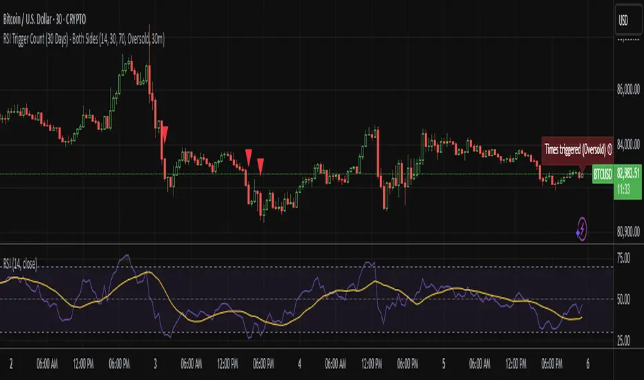
RSI Trigger Count (30 Days) - Both SidesRSI Dual Trigger Counter (30 Days)
This indicator tracks both oversold ( crossunder ) and overbought ( crossover ) RSI events on a 30-minute chart, featuring:
Dual-Mode Selector:
Counts either RSI < 30 (oversold) or RSI > 70 (overbought) crossings
Toggle between modes via input menu
30-Day Rolling Count:
Displays total triggers in the last 30 days (e.g., "Times triggered (Oversold) ① 19")
Visual Alerts:
Red triangles ↓ for oversold crossunders
Green triangles ↑ for overbought crossovers
Customizable:
Adjustable RSI length (2-100) and thresholds (1-100)
Works on any timeframe (auto-scales calculations)
Purpose: Identifies frequent reversal signals for both buying dips (oversold) and selling rallies (overbought).
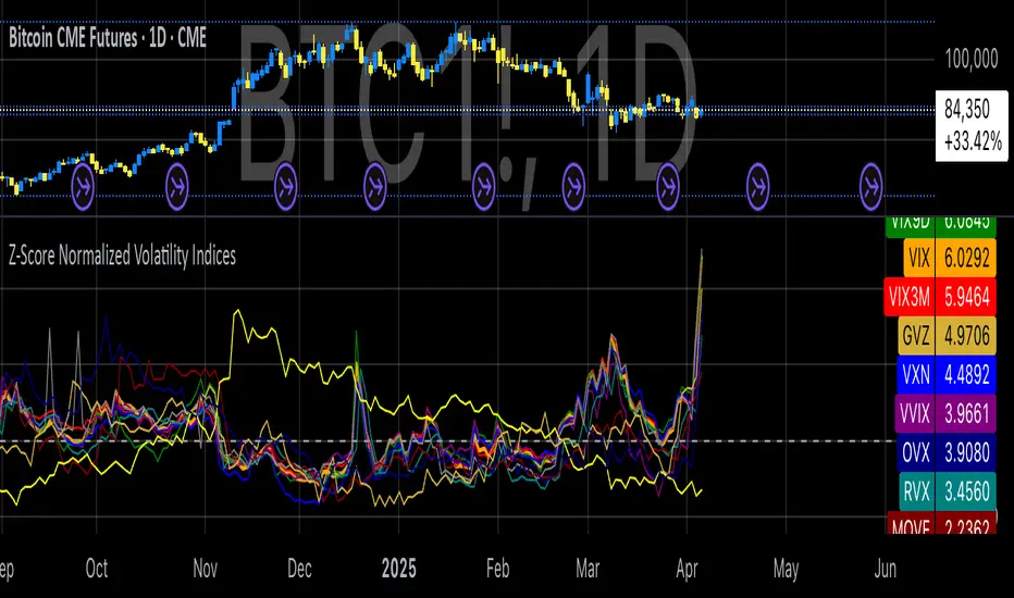
Z-Score Normalized Volatility IndicesVolatility is one of the most important measures in financial markets, reflecting the extent of variation in asset prices over time. It is commonly viewed as a risk indicator, with higher volatility signifying greater uncertainty and potential for price swings, which can affect investment decisions. Understanding volatility and its dynamics is crucial for risk management and forecasting in both traditional and alternative asset classes.
Z-Score Normalization in Volatility Analysis
The Z-score is a statistical tool that quantifies how many standard deviations a given data point is from the mean of the dataset. It is calculated as:
Z = \frac{X - \mu}{\sigma}
Where X is the value of the data point, \mu is the mean of the dataset, and \sigma is the standard deviation of the dataset. In the context of volatility indices, the Z-score allows for the normalization of these values, enabling their comparison regardless of the original scale. This is particularly useful when analyzing volatility across multiple assets or asset classes.
This script utilizes the Z-score to normalize various volatility indices:
1. VIX (CBOE Volatility Index): A widely used indicator that measures the implied volatility of S&P 500 options. It is considered a barometer of market fear and uncertainty (Whaley, 2000).
2. VIX3M: Represents the 3-month implied volatility of the S&P 500 options, providing insight into medium-term volatility expectations.
3. VIX9D: The implied volatility for a 9-day S&P 500 options contract, which reflects short-term volatility expectations.
4. VVIX: The volatility of the VIX itself, which measures the uncertainty in the expectations of future volatility.
5. VXN: The Nasdaq-100 volatility index, representing implied volatility in the Nasdaq-100 options.
6. RVX: The Russell 2000 volatility index, tracking the implied volatility of options on the Russell 2000 Index.
7. VXD: Volatility for the Dow Jones Industrial Average.
8. MOVE: The implied volatility index for U.S. Treasury bonds, offering insight into expectations for interest rate volatility.
9. BVIX: Volatility of Bitcoin options, a useful indicator for understanding the risk in the cryptocurrency market.
10. GVZ: Volatility index for gold futures, reflecting the risk perception of gold prices.
11. OVX: Measures implied volatility for crude oil futures.
Volatility Clustering and Z-Score
The concept of volatility clustering—where high volatility tends to be followed by more high volatility—is well documented in financial literature. This phenomenon is fundamental in volatility modeling and highlights the persistence of periods of heightened market uncertainty (Bollerslev, 1986).
Moreover, studies by Andersen et al. (2012) explore how implied volatility indices, like the VIX, serve as predictors for future realized volatility, underlining the relationship between expected volatility and actual market behavior. The Z-score normalization process helps in making volatility data comparable across different asset classes, enabling more effective decision-making in volatility-based strategies.
Applications in Trading and Risk Management
By using Z-score normalization, traders can more easily assess deviations from the mean in volatility, helping to identify periods when volatility is unusually high or low. This can be used to adjust risk exposure or to implement volatility-based trading strategies, such as mean reversion strategies. Research suggests that volatility mean-reversion is a reliable pattern that can be exploited for profit (Christensen & Prabhala, 1998).
References:
• Andersen, T. G., Bollerslev, T., Diebold, F. X., & Vega, C. (2012). Realized volatility and correlation dynamics: A long-run approach. Journal of Financial Economics, 104(3), 385-406.
• Bollerslev, T. (1986). Generalized autoregressive conditional heteroskedasticity. Journal of Econometrics, 31(3), 307-327.
• Christensen, B. J., & Prabhala, N. R. (1998). The relation between implied and realized volatility. Journal of Financial Economics, 50(2), 125-150.
• Whaley, R. E. (2000). Derivatives on market volatility and the VIX index. Journal of Derivatives, 8(1), 71-84.
RiskCalc FX & GoldRiskCalc FX & Gold is a multi-market position sizing tool designed to help you manage risk quickly and accurately. With this script, simply enter your account capital, the percentage of risk you wish to take, and your stop in ticks. Depending on the selected market—Forex or XAUUSD—the script automatically adjusts its calculations:
Forex: Assumes 1 lot equals 100,000 units.
XAUUSD: Assumes 1 lot equals 100 ounces.
The script calculates your risk in dollars and, using a fixed value of 1 USD per tick per lot, determines the ideal position size in both lots and total contracts. Results are displayed in a clear, centralized table at the top of the chart for real-time decision-making.
Perfect for traders operating across multiple markets who need an automated and consistent approach to risk management.

Oracle Prediction Futur
// (\_/)
// ( •.•)
// (")_(")
Indicator Description: Oracle Prediction Futur
The Oracle Prediction Futur is a sophisticated technical indicator designed for traders and analysts looking to gain insights into market trends through the analysis of price movements. This Pine Script™ code integrates innovative elements to enhance the trading experience and is governed by the Mozilla Public License 2.0.
Key Features:
Normalization of Closing Prices:
The indicator normalizes closing prices over a defined lookback period (100 periods) to provide a percentage-based representation of the current price relative to its historical range. This helps in identifying potential price extremes.
Peak and Trough Detection:
It identifies and plots peak tops and bottom troughs based on normalized closing values. Peak tops are marked with vibrant magenta circles, while peak bottoms are indicated by soothing cyan circles, helping traders visually spot significant turning points in the price action.
Dynamic Background Gradient:
The indicator features a visually appealing gradient background that represents market sentiment. The background color transitions between bear and bull colors based on the position of the normalized close within the 0-100 range. This provides an immediate visual cue about the strength or weakness of the market.
Horizontal Reference Lines:
The indicator includes horizontal lines at key levels (9.51 and 92.5) for quick reference, which can help to gauge areas of potential support or resistance.
User-Friendly Visuals:
The combination of background colors, dynamic plots, and clear labeling offers a user-friendly visual representation, making it easier to interpret market conditions at a glance.
Overlay Options:
As an overlay-free indicator, it maintains clarity on the price chart while providing insightful trends and forecasts.
Practical Application:
Traders can utilize the Oracle Prediction Futur indicator to identify potential entry and exit points in their trading strategies. By observing the peaks, troughs, and background color shifts, users can better understand market momentum and price action.
How to Use:
Deploy this indicator on your trading platform, and analyze the peaks and troughs along with the normalized close line and background gradient to inform your trading decisions. Look for alignment between price action and the signaling provided by the indicator for optimized trading results.

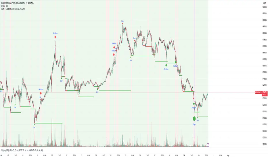
Multi-TF Support LevelsThe Multi-TF Support Levels indicator identifies and displays key support levels based on swing lows across three user-selected timeframes.
How it works:
Input Parameters:
Lookback Period (100) — historical depth to search for swing lows.
Timeframe 1-3 (15, 45, 240) — three timeframes (e.g., 15min, 45min, 4hr).
Logic:
For each timeframe, a swing low is detected: the lowest price within the lookback period that is also lower than the two preceding candles.
Support levels update dynamically when new swing lows are formed.
The most recent levels are plotted as horizontal cross marks (blue, red, green for each timeframe).
Purpose: Visualize significant support zones from multiple timeframes to identify confluent areas for trading decisions.
Индикатор Multi-TF Support Levels (Мультитаймфреймовые уровни поддержки) определяет и отображает ключевые уровни поддержки на основе минимумов свингов (swing lows) на трёх выбранных таймфреймах.
Как работает:
Входные параметры:
Lookback Period (100) — глубина анализа для поиска минимумов.
Timeframe 1-3 (15, 45, 240) — три таймфрейма (например, 15 минут, 45 минут, 4 часа).
Логика:
Для каждого таймфрейма определяется свинг-минимум: цена, которая является самой низкой за период lookback и ниже двух предыдущих свечей.
Уровни поддержки обновляются при появлении новых свинг-минимумов.
Последние актуальные уровни отображаются на графике в виде горизонтальных линий-крестиков (синий, красный, зелёный для каждого таймфрейма).
Цель: Визуализировать значимые уровни поддержки с разных таймфреймов для поиска зон "конфлюэнса".
Multi-Fibonacci Trend Average[FibonacciFlux]Multi-Fibonacci Trend Average (MFTA): An Institutional-Grade Trend Confluence Indicator for Discerning Market Participants
My original indicator/Strategy:
Engineered for the sophisticated demands of institutional and advanced traders, the Multi-Fibonacci Trend Average (MFTA) indicator represents a paradigm shift in technical analysis. This meticulously crafted tool is designed to furnish high-definition trend signals within the complexities of modern financial markets. Anchored in the rigorous principles of Fibonacci ratios and augmented by advanced averaging methodologies, MFTA delivers a granular perspective on trend dynamics. Its integration of Multi-Timeframe (MTF) filters provides unparalleled signal robustness, empowering strategic decision-making with a heightened degree of confidence.
MFTA indicator on BTCUSDT 15min chart with 1min RSI and MACD filters enabled. Note the refined signal generation with reduced noise.
MFTA indicator on BTCUSDT 15min chart without MTF filters. While capturing more potential trading opportunities, it also generates a higher frequency of signals, including potential false positives.
Core Innovation: Proprietary Fibonacci-Enhanced Supertrend Averaging Engine
The MFTA indicator’s core innovation lies in its proprietary implementation of Supertrend analysis, strategically fortified by Fibonacci ratios to construct a truly dynamic volatility envelope. Departing from conventional Supertrend methodologies, MFTA autonomously computes not one, but three distinct Supertrend lines. Each of these lines is uniquely parameterized by a specific Fibonacci factor: 0.618 (Weak), 1.618 (Medium/Golden Ratio), and 2.618 (Strong/Extended Fibonacci).
// Fibonacci-based factors for multiple Supertrend calculations
factor1 = input.float(0.618, 'Factor 1 (Weak/Fibonacci)', minval=0.01, step=0.01, tooltip='Factor 1 (Weak/Fibonacci)', group="Fibonacci Supertrend")
factor2 = input.float(1.618, 'Factor 2 (Medium/Golden Ratio)', minval=0.01, step=0.01, tooltip='Factor 2 (Medium/Golden Ratio)', group="Fibonacci Supertrend")
factor3 = input.float(2.618, 'Factor 3 (Strong/Extended Fib)', minval=0.01, step=0.01, tooltip='Factor 3 (Strong/Extended Fib)', group="Fibonacci Supertrend")
This multi-faceted architecture adeptly captures a spectrum of market volatility sensitivities, ensuring a comprehensive assessment of prevailing conditions. Subsequently, the indicator algorithmically synthesizes these disparate Supertrend lines through arithmetic averaging. To achieve optimal signal fidelity and mitigate inherent market noise, this composite average is further refined utilizing an Exponential Moving Average (EMA).
// Calculate average of the three supertends and a smoothed version
superlength = input.int(21, 'Smoothing Length', tooltip='Smoothing Length for Average Supertrend', group="Fibonacci Supertrend")
average_trend = (supertrend1 + supertrend2 + supertrend3) / 3
smoothed_trend = ta.ema(average_trend, superlength)
The resultant ‘Smoothed Trend’ line emerges as a remarkably responsive yet stable trend demarcation, offering demonstrably superior clarity and precision compared to singular Supertrend implementations, particularly within the turbulent dynamics of high-volatility markets.
Elevated Signal Confluence: Integrated Multi-Timeframe (MTF) Validation Suite
MFTA transcends the limitations of conventional trend indicators by incorporating an advanced suite of three independent MTF filters: RSI, MACD, and Volume. These filters function as sophisticated validation protocols, rigorously ensuring that only signals exhibiting a confluence of high-probability factors are brought to the forefront.
1. Granular Lower Timeframe RSI Momentum Filter
The Relative Strength Index (RSI) filter, computed from a user-defined lower timeframe, furnishes critical momentum-based signal validation. By meticulously monitoring RSI dynamics on an accelerated timeframe, traders gain the capacity to evaluate underlying momentum strength with precision, prior to committing to signal execution on the primary chart timeframe.
// --- Lower Timeframe RSI Filter ---
ltf_rsi_filter_enable = input.bool(false, title="Enable RSI Filter", group="MTF Filters", tooltip="Use RSI from lower timeframe as a filter")
ltf_rsi_timeframe = input.timeframe("1", title="RSI Timeframe", group="MTF Filters", tooltip="Timeframe for RSI calculation")
ltf_rsi_length = input.int(14, title="RSI Length", minval=1, group="MTF Filters", tooltip="Length for RSI calculation")
ltf_rsi_threshold = input.int(30, title="RSI Threshold", minval=0, maxval=100, group="MTF Filters", tooltip="RSI value threshold for filtering signals")
2. Convergent Lower Timeframe MACD Trend-Momentum Filter
The Moving Average Convergence Divergence (MACD) filter, also calculated on a lower timeframe basis, introduces a critical layer of trend-momentum convergence confirmation. The bullish signal configuration rigorously mandates that the MACD line be definitively positioned above the Signal line on the designated lower timeframe. This stringent condition ensures a robust indication of converging momentum that aligns synergistically with the prevailing trend identified on the primary timeframe.
// --- Lower Timeframe MACD Filter ---
ltf_macd_filter_enable = input.bool(false, title="Enable MACD Filter", group="MTF Filters", tooltip="Use MACD from lower timeframe as a filter")
ltf_macd_timeframe = input.timeframe("1", title="MACD Timeframe", group="MTF Filters", tooltip="Timeframe for MACD calculation")
ltf_macd_fast_length = input.int(12, title="MACD Fast Length", minval=1, group="MTF Filters", tooltip="Fast EMA length for MACD")
ltf_macd_slow_length = input.int(26, title="MACD Slow Length", minval=1, group="MTF Filters", tooltip="Slow EMA length for MACD")
ltf_macd_signal_length = input.int(9, title="MACD Signal Length", minval=1, group="MTF Filters", tooltip="Signal SMA length for MACD")
3. Definitive Volume Confirmation Filter
The Volume Filter functions as an indispensable arbiter of trade conviction. By establishing a dynamic volume threshold, defined as a percentage relative to the average volume over a user-specified lookback period, traders can effectively ensure that all generated signals are rigorously validated by demonstrably increased trading activity. This pivotal validation step signifies robust market participation, substantially diminishing the potential for spurious or false breakout signals.
// --- Volume Filter ---
volume_filter_enable = input.bool(false, title="Enable Volume Filter", group="MTF Filters", tooltip="Use volume level as a filter")
volume_threshold_percent = input.int(title="Volume Threshold (%)", defval=150, minval=100, group="MTF Filters", tooltip="Minimum volume percentage compared to average volume to allow signal (100% = average)")
These meticulously engineered filters operate in synergistic confluence, requiring all enabled filters to definitively satisfy their pre-defined conditions before a Buy or Sell signal is generated. This stringent multi-layered validation process drastically minimizes the incidence of false positive signals, thereby significantly enhancing entry precision and overall signal reliability.
Intuitive Visual Architecture & Actionable Intelligence
MFTA provides a demonstrably intuitive and visually rich charting environment, meticulously delineating trend direction and momentum through precisely color-coded plots:
Average Supertrend: Thin line, green/red for uptrend/downtrend, immediate directional bias.
Smoothed Supertrend: Bold line, teal/purple for uptrend/downtrend, cleaner, institutionally robust trend.
Dynamic Trend Fill: Green/red fill between Supertrends quantifies trend strength and momentum.
Adaptive Background Coloring: Light green/red background mirrors Smoothed Supertrend direction, holistic trend perspective.
Precision Buy/Sell Signals: ‘BUY’/‘SELL’ labels appear on chart when trend touch and MTF filter confluence are satisfied, facilitating high-conviction trade action.
MFTA indicator applied to BTCUSDT 4-hour chart, showcasing its effectiveness on higher timeframes. The Smoothed Length parameter is increased to 200 for enhanced smoothness on this timeframe, coupled with 1min RSI and Volume filters for signal refinement. This illustrates the indicator's adaptability across different timeframes and market conditions.
Strategic Applications for Institutional Mandates
MFTA’s sophisticated design provides distinct advantages for advanced trading operations and institutional investment mandates. Key strategic applications include:
High-Probability Trend Identification: Fibonacci-averaged Supertrend with MTF filters robustly identifies high-probability trend continuations and reversals, enhancing alpha generation.
Precision Entry/Exit Signals: Volume and momentum-filtered signals enable institutional-grade precision for optimized risk-adjusted returns.
Algorithmic Trading Integration: Clear signal logic facilitates seamless integration into automated trading systems for scalable strategy deployment.
Multi-Asset/Timeframe Versatility: Adaptable parameters ensure applicability across diverse asset classes and timeframes, catering to varied trading mandates.
Enhanced Risk Management: Superior signal fidelity from MTF filters inherently reduces false signals, supporting robust risk management protocols.
Granular Customization and Parameterized Control
MFTA offers unparalleled customization, empowering users to fine-tune parameters for precise alignment with specific trading styles and market conditions. Key adjustable parameters include:
Fibonacci Factors: Adjust Supertrend sensitivity to volatility regimes.
ATR Length: Control volatility responsiveness in Supertrend calculations.
Smoothing Length: Refine Smoothed Trend line responsiveness and noise reduction.
MTF Filter Parameters: Independently configure timeframes, lookback periods, and thresholds for RSI, MACD, and Volume filters for optimal signal filtering.
Disclaimer
MFTA is meticulously engineered for high-quality trend signals; however, no indicator guarantees profit. Market conditions are unpredictable, and trading involves substantial risk. Rigorous backtesting and forward testing across diverse datasets, alongside a comprehensive understanding of the indicator's logic, are essential before live deployment. Past performance is not indicative of future results. MFTA is for informational and analytical purposes only and is not financial or investment advice.
