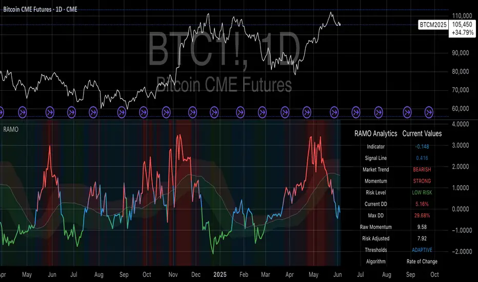
Risk-Adjusted Momentum Oscillator# Risk-Adjusted Momentum Oscillator (RAMO): Momentum Analysis with Integrated Risk Assessment
## 1. Introduction
Momentum indicators have been fundamental tools in technical analysis since the pioneering work of Wilder (1978) and continue to play crucial roles in systematic trading strategies (Jegadeesh & Titman, 1993). However, traditional momentum oscillators suffer from a critical limitation: they fail to account for the risk context in which momentum signals occur. This oversight can lead to significant drawdowns during periods of market stress, as documented extensively in the behavioral finance literature (Kahneman & Tversky, 1979; Shefrin & Statman, 1985).
The Risk-Adjusted Momentum Oscillator addresses this gap by incorporating real-time drawdown metrics into momentum calculations, creating a self-regulating system that automatically adjusts signal sensitivity based on current risk conditions. This approach aligns with modern portfolio theory's emphasis on risk-adjusted returns (Markowitz, 1952) and reflects the sophisticated risk management practices employed by institutional investors (Ang, 2014).
## 2. Theoretical Foundation
### 2.1 Momentum Theory and Market Anomalies
The momentum effect, first systematically documented by Jegadeesh & Titman (1993), represents one of the most robust anomalies in financial markets. Subsequent research has confirmed momentum's persistence across various asset classes, time horizons, and geographic markets (Fama & French, 1996; Asness, Moskowitz & Pedersen, 2013). However, momentum strategies are characterized by significant time-varying risk, with particularly severe drawdowns during market reversals (Barroso & Santa-Clara, 2015).
### 2.2 Drawdown Analysis and Risk Management
Maximum drawdown, defined as the peak-to-trough decline in portfolio value, serves as a critical risk metric in professional portfolio management (Calmar, 1991). Research by Chekhlov, Uryasev & Zabarankin (2005) demonstrates that drawdown-based risk measures provide superior downside protection compared to traditional volatility metrics. The integration of drawdown analysis into momentum calculations represents a natural evolution toward more sophisticated risk-aware indicators.
### 2.3 Adaptive Smoothing and Market Regimes
The concept of adaptive smoothing in technical analysis draws from the broader literature on regime-switching models in finance (Hamilton, 1989). Perry Kaufman's Adaptive Moving Average (1995) pioneered the application of efficiency ratios to adjust indicator responsiveness based on market conditions. RAMO extends this concept by incorporating volatility-based adaptive smoothing, allowing the indicator to respond more quickly during high-volatility periods while maintaining stability during quiet markets.
## 3. Methodology
### 3.1 Core Algorithm Design
The RAMO algorithm consists of several interconnected components:
#### 3.1.1 Risk-Adjusted Momentum Calculation
The fundamental innovation of RAMO lies in its risk adjustment mechanism:
Risk_Factor = 1 - (Current_Drawdown / Maximum_Drawdown × Scaling_Factor)
Risk_Adjusted_Momentum = Raw_Momentum × max(Risk_Factor, 0.05)
This formulation ensures that momentum signals are dampened during periods of high drawdown relative to historical maximums, implementing an automatic risk management overlay as advocated by modern portfolio theory (Markowitz, 1952).
#### 3.1.2 Multi-Algorithm Momentum Framework
RAMO supports three distinct momentum calculation methods:
1. Rate of Change: Traditional percentage-based momentum (Pring, 2002)
2. Price Momentum: Absolute price differences
3. Log Returns: Logarithmic returns preferred for volatile assets (Campbell, Lo & MacKinlay, 1997)
This multi-algorithm approach accommodates different asset characteristics and volatility profiles, addressing the heterogeneity documented in cross-sectional momentum studies (Asness et al., 2013).
### 3.2 Leading Indicator Components
#### 3.2.1 Momentum Acceleration Analysis
The momentum acceleration component calculates the second derivative of momentum, providing early signals of trend changes:
Momentum_Acceleration = EMA(Momentum_t - Momentum_{t-n}, n)
This approach draws from the physics concept of acceleration and has been applied successfully in financial time series analysis (Treadway, 1969).
#### 3.2.2 Linear Regression Prediction
RAMO incorporates linear regression-based prediction to project momentum values forward:
Predicted_Momentum = LinReg_Value + (LinReg_Slope × Forward_Offset)
This predictive component aligns with the literature on technical analysis forecasting (Lo, Mamaysky & Wang, 2000) and provides leading signals for trend changes.
#### 3.2.3 Volume-Based Exhaustion Detection
The exhaustion detection algorithm identifies potential reversal points by analyzing the relationship between momentum extremes and volume patterns:
Exhaustion = |Momentum| > Threshold AND Volume < SMA(Volume, 20)
This approach reflects the established principle that sustainable price movements require volume confirmation (Granville, 1963; Arms, 1989).
### 3.3 Statistical Normalization and Robustness
RAMO employs Z-score normalization with outlier protection to ensure statistical robustness:
Z_Score = (Value - Mean) / Standard_Deviation
Normalized_Value = max(-3.5, min(3.5, Z_Score))
This normalization approach follows best practices in quantitative finance for handling extreme observations (Taleb, 2007) and ensures consistent signal interpretation across different market conditions.
### 3.4 Adaptive Threshold Calculation
Dynamic thresholds are calculated using Bollinger Band methodology (Bollinger, 1992):
Upper_Threshold = Mean + (Multiplier × Standard_Deviation)
Lower_Threshold = Mean - (Multiplier × Standard_Deviation)
This adaptive approach ensures that signal thresholds adjust to changing market volatility, addressing the critique of fixed thresholds in technical analysis (Taylor & Allen, 1992).
## 4. Implementation Details
### 4.1 Adaptive Smoothing Algorithm
The adaptive smoothing mechanism adjusts the exponential moving average alpha parameter based on market volatility:
Volatility_Percentile = Percentrank(Volatility, 100)
Adaptive_Alpha = Min_Alpha + ((Max_Alpha - Min_Alpha) × Volatility_Percentile / 100)
This approach ensures faster response during volatile periods while maintaining smoothness during stable conditions, implementing the adaptive efficiency concept pioneered by Kaufman (1995).
### 4.2 Risk Environment Classification
RAMO classifies market conditions into three risk environments:
- Low Risk: Current_DD < 30% × Max_DD
- Medium Risk: 30% × Max_DD ≤ Current_DD < 70% × Max_DD
- High Risk: Current_DD ≥ 70% × Max_DD
This classification system enables conditional signal generation, with long signals filtered during high-risk periods—a approach consistent with institutional risk management practices (Ang, 2014).
## 5. Signal Generation and Interpretation
### 5.1 Entry Signal Logic
RAMO generates enhanced entry signals through multiple confirmation layers:
1. Primary Signal: Crossover between indicator and signal line
2. Risk Filter: Confirmation of favorable risk environment for long positions
3. Leading Component: Early warning signals via acceleration analysis
4. Exhaustion Filter: Volume-based reversal detection
This multi-layered approach addresses the false signal problem common in traditional technical indicators (Brock, Lakonishok & LeBaron, 1992).
### 5.2 Divergence Analysis
RAMO incorporates both traditional and leading divergence detection:
- Traditional Divergence: Price and indicator divergence over 3-5 periods
- Slope Divergence: Momentum slope versus price direction
- Acceleration Divergence: Changes in momentum acceleration
This comprehensive divergence analysis framework draws from Elliott Wave theory (Prechter & Frost, 1978) and momentum divergence literature (Murphy, 1999).
## 6. Empirical Advantages and Applications
### 6.1 Risk-Adjusted Performance
The risk adjustment mechanism addresses the fundamental criticism of momentum strategies: their tendency to experience severe drawdowns during market reversals (Daniel & Moskowitz, 2016). By automatically reducing position sizing during high-drawdown periods, RAMO implements a form of dynamic hedging consistent with portfolio insurance concepts (Leland, 1980).
### 6.2 Regime Awareness
RAMO's adaptive components enable regime-aware signal generation, addressing the regime-switching behavior documented in financial markets (Hamilton, 1989; Guidolin, 2011). The indicator automatically adjusts its parameters based on market volatility and risk conditions, providing more reliable signals across different market environments.
### 6.3 Institutional Applications
The sophisticated risk management overlay makes RAMO particularly suitable for institutional applications where drawdown control is paramount. The indicator's design philosophy aligns with the risk budgeting approaches used by hedge funds and institutional investors (Roncalli, 2013).
## 7. Limitations and Future Research
### 7.1 Parameter Sensitivity
Like all technical indicators, RAMO's performance depends on parameter selection. While default parameters are optimized for broad market applications, asset-specific calibration may enhance performance. Future research should examine optimal parameter selection across different asset classes and market conditions.
### 7.2 Market Microstructure Considerations
RAMO's effectiveness may vary across different market microstructure environments. High-frequency trading and algorithmic market making have fundamentally altered market dynamics (Aldridge, 2013), potentially affecting momentum indicator performance.
### 7.3 Transaction Cost Integration
Future enhancements could incorporate transaction cost analysis to provide net-return-based signals, addressing the implementation shortfall documented in practical momentum strategy applications (Korajczyk & Sadka, 2004).
## References
Aldridge, I. (2013). *High-Frequency Trading: A Practical Guide to Algorithmic Strategies and Trading Systems*. 2nd ed. Hoboken, NJ: John Wiley & Sons.
Ang, A. (2014). *Asset Management: A Systematic Approach to Factor Investing*. New York: Oxford University Press.
Arms, R. W. (1989). *The Arms Index (TRIN): An Introduction to the Volume Analysis of Stock and Bond Markets*. Homewood, IL: Dow Jones-Irwin.
Asness, C. S., Moskowitz, T. J., & Pedersen, L. H. (2013). Value and momentum everywhere. *Journal of Finance*, 68(3), 929-985.
Barroso, P., & Santa-Clara, P. (2015). Momentum has its moments. *Journal of Financial Economics*, 116(1), 111-120.
Bollinger, J. (1992). *Bollinger on Bollinger Bands*. New York: McGraw-Hill.
Brock, W., Lakonishok, J., & LeBaron, B. (1992). Simple technical trading rules and the stochastic properties of stock returns. *Journal of Finance*, 47(5), 1731-1764.
Calmar, T. (1991). The Calmar ratio: A smoother tool. *Futures*, 20(1), 40.
Campbell, J. Y., Lo, A. W., & MacKinlay, A. C. (1997). *The Econometrics of Financial Markets*. Princeton, NJ: Princeton University Press.
Chekhlov, A., Uryasev, S., & Zabarankin, M. (2005). Drawdown measure in portfolio optimization. *International Journal of Theoretical and Applied Finance*, 8(1), 13-58.
Daniel, K., & Moskowitz, T. J. (2016). Momentum crashes. *Journal of Financial Economics*, 122(2), 221-247.
Fama, E. F., & French, K. R. (1996). Multifactor explanations of asset pricing anomalies. *Journal of Finance*, 51(1), 55-84.
Granville, J. E. (1963). *Granville's New Key to Stock Market Profits*. Englewood Cliffs, NJ: Prentice-Hall.
Guidolin, M. (2011). Markov switching models in empirical finance. In D. N. Drukker (Ed.), *Missing Data Methods: Time-Series Methods and Applications* (pp. 1-86). Bingley: Emerald Group Publishing.
Hamilton, J. D. (1989). A new approach to the economic analysis of nonstationary time series and the business cycle. *Econometrica*, 57(2), 357-384.
Jegadeesh, N., & Titman, S. (1993). Returns to buying winners and selling losers: Implications for stock market efficiency. *Journal of Finance*, 48(1), 65-91.
Kahneman, D., & Tversky, A. (1979). Prospect theory: An analysis of decision under risk. *Econometrica*, 47(2), 263-291.
Kaufman, P. J. (1995). *Smarter Trading: Improving Performance in Changing Markets*. New York: McGraw-Hill.
Korajczyk, R. A., & Sadka, R. (2004). Are momentum profits robust to trading costs? *Journal of Finance*, 59(3), 1039-1082.
Leland, H. E. (1980). Who should buy portfolio insurance? *Journal of Finance*, 35(2), 581-594.
Lo, A. W., Mamaysky, H., & Wang, J. (2000). Foundations of technical analysis: Computational algorithms, statistical inference, and empirical implementation. *Journal of Finance*, 55(4), 1705-1765.
Markowitz, H. (1952). Portfolio selection. *Journal of Finance*, 7(1), 77-91.
Murphy, J. J. (1999). *Technical Analysis of the Financial Markets: A Comprehensive Guide to Trading Methods and Applications*. New York: New York Institute of Finance.
Prechter, R. R., & Frost, A. J. (1978). *Elliott Wave Principle: Key to Market Behavior*. Gainesville, GA: New Classics Library.
Pring, M. J. (2002). *Technical Analysis Explained: The Successful Investor's Guide to Spotting Investment Trends and Turning Points*. 4th ed. New York: McGraw-Hill.
Roncalli, T. (2013). *Introduction to Risk Parity and Budgeting*. Boca Raton, FL: CRC Press.
Shefrin, H., & Statman, M. (1985). The disposition to sell winners too early and ride losers too long: Theory and evidence. *Journal of Finance*, 40(3), 777-790.
Taleb, N. N. (2007). *The Black Swan: The Impact of the Highly Improbable*. New York: Random House.
Taylor, M. P., & Allen, H. (1992). The use of technical analysis in the foreign exchange market. *Journal of International Money and Finance*, 11(3), 304-314.
Treadway, A. B. (1969). On rational entrepreneurial behavior and the demand for investment. *Review of Economic Studies*, 36(2), 227-239.
Wilder, J. W. (1978). *New Concepts in Technical Trading Systems*. Greensboro, NC: Trend Research.
"摩根纳斯达克100基金风险大吗" için komut dosyalarını ara
Options Risk Manager v2.2.0 - Priority 7 CompleteScript Description for TradingView Publication
Options Risk Manager v2.2.0 - Priority 7 Complete
What does this script do?
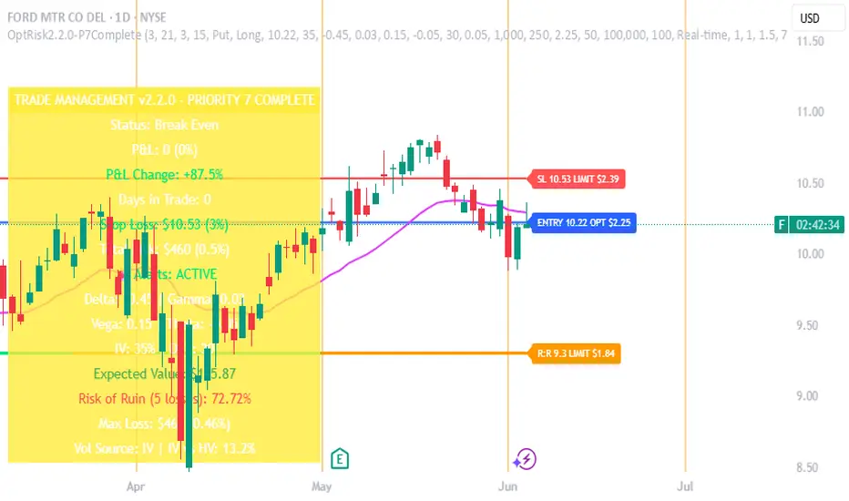
Options Risk Manager v2.2.0 is a comprehensive position management system designed specifically for options traders. The indicator calculates precise stop loss levels, risk/reward targets, and position sizing based on user-defined risk parameters. It provides real-time profit/loss tracking, options Greeks monitoring, and automated alert systems for critical price levels.
The script displays entry points, stop losses, and profit targets directly on the chart while continuously calculating position metrics including dollar risk, account exposure, and probability of success. Version 2.2.0 introduces Priority 7 advanced alerts with dynamic risk warnings and multi-condition notifications.
How does it do it?
The script performs several key calculations:
1. Risk-Based Stop Loss Calculation - Determines stop loss levels based on percentage of entry price, automatically adjusting for calls versus puts. Put positions place stops above entry, while calls place stops below.
2. Position Sizing Algorithm - Calculates optimal contract quantities using account size, risk
percentage, and stop distance to ensure consistent risk per trade regardless of underlying price.
3. Options-Specific P&L Tracking - Incorporates Delta, Gamma, Vega, and Theta to provide accurate profit/loss calculations for options positions, including time decay effects.
4. Three-Phase Trade Management - Implements systematic position management through Entry
Phase (initial risk), Profit Phase (approaching target), and Trailing Phase (EMA-based exit
management).
5. Multi-Level Alert System - Monitors price action, Greeks thresholds, time decay acceleration, and account risk levels to generate context-aware notifications.
How to use it?
Initial Setup:
1. Apply indicator to any optionable security
2. Toggle "In Position" ON when entering a trade
3. Set Direction (Call/Put) and Side (Long/Short)
4. Enter the underlying price at position entry
5. Specify number of contracts and risk percentage
Position Management:
Blue line shows entry price
Red line indicates stop loss level
Orange line displays risk/reward target
Purple EMA line activates after target hit
Monitor real-time P&L in trade panels
Alert Configuration:
Enable Advanced Alerts in settings
Set profit/loss notification thresholds
Configure Greek-based warnings
Activate time decay alerts for expiration
Risk Parameters:
Risk % determines stop distance from entry
Account Value sets position sizing limits
Contract Multiplier (standard = 100)
R:R Ratio defines profit targets
What makes it unique?
Options Risk Manager addresses the specific challenges of options trading that generic indicators miss. The script accounts for the inverse relationship in put options (profiting from price declines), incorporates Greeks for accurate P&L calculations, and provides options-specific limit orders for TradeStation integration.
The three-phase management system removes emotional decision-making by defining clear rules for position management. Phase transitions occur automatically based on price action, shifting from initial risk management to profit protection to trend-following modes.
Version 2.2.0's Priority 7 alert system provides intelligent notifications that include live metrics, risk warnings, and market context rather than simple price crosses.
Key Features Summary
Options-Specific Calculations - Proper handling of calls/puts with inverse relationships
Risk-Based Position Sizing - Consistent risk regardless of underlying price
Greeks Integration - Delta, Gamma, Vega, Theta for accurate tracking
Phase Management System - Systematic three-stage position handling
Advanced Alert System - Context-aware notifications with metrics
TradeStation Integration - Option limit orders for execution
Visual Risk Display - Clear chart overlays for all levels
Probability Calculator - Win/loss probability with expected value
Multi-Account Support - Scales from small to large accounts
Important Notes
This indicator requires manual input of option prices and Greeks (available from your broker's option chain). It functions as a risk management overlay and does not generate entry signals. The calculations assume standard options contracts of 100 shares.
Designed for TradeStation platform with full functionality. Basic features available on other platforms
without options data integration. Always verify calculations with your broker's risk system before placing
trades.
RSI-Adaptive T3 [ChartPrime]The RSI-Adaptive T3 is a precision trend-following tool built around the legendary T3 smoothing algorithm developed by Tim Tillson , designed to enhance responsiveness while reducing lag compared to traditional moving averages. Current implementation takes it a step further by dynamically adapting the smoothing length based on real-time RSI conditions — allowing the T3 to “breathe” with market volatility. This dynamic length makes the curve faster in trending moves and smoother during consolidations.
To help traders visualize volatility and directional momentum, adaptive volatility bands are plotted around the T3 line, with visual crossover markers and a dynamic info panel on the chart. It’s ideal for identifying trend shifts, spotting momentum surges, and adapting strategy execution to the pace of the market.
HOIW IT WORKS
At its core, this indicator fuses two ideas:
The T3 Moving Average — a 6-stage recursively smoothed exponential average created by Tim Tillson , designed to reduce lag without sacrificing smoothness. It uses a volume factor to control curvature.
A Dynamic Length Engine — powered by the RSI. When RSI is low (market oversold), the T3 becomes shorter and more reactive. When RSI is high (overbought), the T3 becomes longer and smoother. This creates a feedback loop between price momentum and trend sensitivity.
// Step 1: Adaptive length via RSI
rsi = ta.rsi(src, rsiLen)
rsi_scale = 1 - rsi / 100
len = math.round(minLen + (maxLen - minLen) * rsi_scale)
pine_ema(src, length) =>
alpha = 2 / (length + 1)
sum = 0.0
sum := na(sum ) ? src : alpha * src + (1 - alpha) * nz(sum )
sum
// Step 2: T3 with adaptive length
e1 = pine_ema(src, len)
e2 = pine_ema(e1, len)
e3 = pine_ema(e2, len)
e4 = pine_ema(e3, len)
e5 = pine_ema(e4, len)
e6 = pine_ema(e5, len)
c1 = -v * v * v
c2 = 3 * v * v + 3 * v * v * v
c3 = -6 * v * v - 3 * v - 3 * v * v * v
c4 = 1 + 3 * v + v * v * v + 3 * v * v
t3 = c1 * e6 + c2 * e5 + c3 * e4 + c4 * e3
The result: an evolving trend line that adapts to market tempo in real-time.
KEY FEATURES
⯁ RSI-Based Adaptive Smoothing
The length of the T3 calculation dynamically adjusts between a Min Length and Max Length , based on the current RSI.
When RSI is low → the T3 shortens, tracking reversals faster.
When RSI is high → the T3 stretches, filtering out noise during euphoria phases.
Displayed length is shown in a floating table, colored on a gradient between min/max values.
⯁ T3 Calculation (Tim Tillson Method)
The script uses a 6-stage EMA cascade with a customizable Volume Factor (v) , as designed by Tillson (1998) .
Formula:
T3 = c1 * e6 + c2 * e5 + c3 * e4 + c4 * e3
This technique gives smoother yet faster curves than EMAs or DEMA/Triple EMA.
⯁ Visual Trend Direction & Transitions
The T3 line changes color dynamically:
Color Up (default: blue) → bullish curvature
Color Down (default: orange) → bearish curvature
Plot fill between T3 and delayed T3 creates a gradient ribbon to show momentum expansion/contraction.
Directional shift markers (“🞛”) are plotted when T3 crosses its own delayed value — helping traders spot trend flips or pullback entries.
⯁ Adaptive Volatility Bands
Optional upper/lower bands are plotted around the T3 line using a user-defined volatility window (default: 100).
Bands widen when volatility rises, and contract during compression — similar to Bollinger logic but centered on the adaptive T3.
Shaded band zones help frame breakout setups or mean-reversion zones.
⯁ Dynamic Info Table
A live stats panel shows:
Current adaptive length
Maximum smoothing (▲ MaxLen)
Minimum smoothing (▼ MinLen)
All values update in real time and are color-coded to match trend direction.
HOW TO USE
Use T3 crossovers to detect trend transitions, especially during periods of volatility compression.
Watch for volatility contraction in the bands — breakouts from narrow band periods often precede trend bursts.
The adaptive smoothing length can also be used to assess current market tempo — tighter = faster; wider = slower.
CONCLUSION
RSI-Adaptive T3 modernizes one of the most elegant smoothing algorithms in technical analysis with intelligent RSI responsiveness and built-in volatility bands. It gives traders a cleaner read on trend health, directional shifts, and expansion dynamics — all in a visually efficient package. Perfect for scalpers, swing traders, and algorithmic modelers alike, it delivers advanced logic in a plug-and-play format.

VIDYA (Chande)This script brings you VIDYA – the Variable Index Dynamic Average, developed by Tushar Chande. It’s not your typical moving average. Unlike the standard SMA or EMA, VIDYA adapts its speed and smoothness based on real-time market momentum using the Chande Momentum Oscillator (CMO).
Think of it like a moving average that gets faster during strong trends and slows down during sideways or choppy markets — just like how a smart trader would!
🧠 What Makes VIDYA Different?
Traditional moving averages use fixed smoothing, so they lag more during big moves or chop during weak trends.
VIDYA fixes that by adapting its behavior dynamically:
When momentum is strong → VIDYA reacts faster 🚀
When momentum is weak → VIDYA smooths out the noise 🧘
⚙️ How It Works (Explained Simply):
1️⃣ CMO Calculation (Chande Momentum Oscillator):
We look at the past cmoLength candles (default 9) and:
i) Add up all the positive price changes (gains)
ii) Add up all the negative price changes (losses)
iii) Use those to compute a normalized momentum score between -100 and +100
📌 CMO = (Gains - Losses) / (Gains + Losses)
• This gives us a momentum reading that powers the next step.
2️⃣ Dynamic Alpha Smoothing:
• We convert the absolute value of the CMO into an alpha — this is the "speed" of the VIDYA.
📌 Higher momentum = higher alpha → faster response
📌 Lower momentum = lower alpha → smoother behavior
3️⃣ VIDYA Formula:
• Finally, we apply the smoothing:
📌 VIDYA = α × Price + (1 - α) × Previous VIDYA
• This equation continuously adapts to market behavior — trending or ranging.
📊 What’s Plotted?
🟠 The VIDYA Line:
A smooth, responsive line plotted on your price chart that adjusts in real-time with price momentum.
🔎 How to Use It:
✅ Use it like a moving average, but smarter:
• Price > VIDYA and rising → Trend is likely up
• Price < VIDYA and falling → Trend is likely down
• Flat VIDYA = Possible consolidation or sideways market
✅ Combine with:
• Breakout strategies (VIDYA confirms momentum)
• Reversal entries (look for price crossing VIDYA)
• Volatility filters (ignore signals when VIDYA flattens)
🧪 Bonus Tip:
Pair this with a volume indicator (like my Volume Confirmation Bars or Volume Strength Highlight) to confirm whether momentum is backed by real participation or just a fakeout.
📩 Want alerts, dual-timeframe overlays, or VIDYA with other base inputs (like typical price or HLC3)? Let me know — happy to expand this for your setup!
Stay adaptive, not reactive — trade smarter with VIDYA! 🧠📉📈

Advanced Petroleum Market Model (APMM)Advanced Petroleum Market Model (APMM): A Multi-Factor Fundamental Analysis Framework for Oil Market Assessment
## 1. Introduction
The petroleum market represents one of the most complex and globally significant commodity markets, characterized by intricate supply-demand dynamics, geopolitical influences, and substantial price volatility (Hamilton, 2009). Traditional fundamental analysis approaches often struggle to synthesize the multitude of relevant indicators into actionable insights due to data heterogeneity, temporal misalignment, and subjective weighting schemes (Baumeister & Kilian, 2016).
The Advanced Petroleum Market Model addresses these limitations through a systematic, quantitative approach that integrates 16 verified fundamental indicators across five critical market dimensions. The model builds upon established financial engineering principles while incorporating petroleum-specific market dynamics and adaptive learning mechanisms.
## 2. Theoretical Framework
### 2.1 Market Efficiency and Information Integration
The model operates under the assumption of semi-strong market efficiency, where fundamental information is gradually incorporated into prices with varying degrees of lag (Fama, 1970). The petroleum market's unique characteristics, including storage costs, transportation constraints, and geopolitical risk premiums, create opportunities for fundamental analysis to provide predictive value (Kilian, 2009).
### 2.2 Multi-Factor Asset Pricing Theory
Drawing from Ross's (1976) Arbitrage Pricing Theory, the model treats petroleum prices as driven by multiple systematic risk factors. The five-factor decomposition (Supply, Inventory, Demand, Trade, Sentiment) represents economically meaningful sources of systematic risk in petroleum markets (Chen et al., 1986).
## 3. Methodology
### 3.1 Data Sources and Quality Framework
The model integrates 16 fundamental indicators sourced from verified TradingView economic data feeds:
Supply Indicators:
- US Oil Production (ECONOMICS:USCOP)
- US Oil Rigs Count (ECONOMICS:USCOR)
- API Crude Runs (ECONOMICS:USACR)
Inventory Indicators:
- US Crude Stock Changes (ECONOMICS:USCOSC)
- Cushing Stocks (ECONOMICS:USCCOS)
- API Crude Stocks (ECONOMICS:USCSC)
- API Gasoline Stocks (ECONOMICS:USGS)
- API Distillate Stocks (ECONOMICS:USDS)
Demand Indicators:
- Refinery Crude Runs (ECONOMICS:USRCR)
- Gasoline Production (ECONOMICS:USGPRO)
- Distillate Production (ECONOMICS:USDFP)
- Industrial Production Index (FRED:INDPRO)
Trade Indicators:
- US Crude Imports (ECONOMICS:USCOI)
- US Oil Exports (ECONOMICS:USOE)
- API Crude Imports (ECONOMICS:USCI)
- Dollar Index (TVC:DXY)
Sentiment Indicators:
- Oil Volatility Index (CBOE:OVX)
### 3.2 Data Quality Monitoring System
Following best practices in quantitative finance (Lopez de Prado, 2018), the model implements comprehensive data quality monitoring:
Data Quality Score = Σ(Individual Indicator Validity) / Total Indicators
Where validity is determined by:
- Non-null data availability
- Positive value validation
- Temporal consistency checks
### 3.3 Statistical Normalization Framework
#### 3.3.1 Z-Score Normalization
The model employs robust Z-score normalization as established by Sharpe (1994) for cross-indicator comparability:
Z_i,t = (X_i,t - μ_i) / σ_i
Where:
- X_i,t = Raw value of indicator i at time t
- μ_i = Sample mean of indicator i
- σ_i = Sample standard deviation of indicator i
Z-scores are capped at ±3 to mitigate outlier influence (Tukey, 1977).
#### 3.3.2 Percentile Rank Transformation
For intuitive interpretation, Z-scores are converted to percentile ranks following the methodology of Conover (1999):
Percentile_Rank = (Number of values < current_value) / Total_observations × 100
### 3.4 Exponential Smoothing Framework
Signal smoothing employs exponential weighted moving averages (Brown, 1963) with adaptive alpha parameter:
S_t = α × X_t + (1-α) × S_{t-1}
Where α = 2/(N+1) and N represents the smoothing period.
### 3.5 Dynamic Threshold Optimization
The model implements adaptive thresholds using Bollinger Band methodology (Bollinger, 1992):
Dynamic_Threshold = μ ± (k × σ)
Where k is the threshold multiplier adjusted for market volatility regime.
### 3.6 Composite Score Calculation
The fundamental score integrates component scores through weighted averaging:
Fundamental_Score = Σ(w_i × Score_i × Quality_i)
Where:
- w_i = Normalized component weight
- Score_i = Component fundamental score
- Quality_i = Data quality adjustment factor
## 4. Implementation Architecture
### 4.1 Adaptive Parameter Framework
The model incorporates regime-specific adjustments based on market volatility:
Volatility_Regime = σ_price / μ_price × 100
High volatility regimes (>25%) trigger enhanced weighting for inventory and sentiment components, reflecting increased market sensitivity to supply disruptions and psychological factors.
### 4.2 Data Synchronization Protocol
Given varying publication frequencies (daily, weekly, monthly), the model employs forward-fill synchronization to maintain temporal alignment across all indicators.
### 4.3 Quality-Adjusted Scoring
Component scores are adjusted for data quality to prevent degraded inputs from contaminating the composite signal:
Adjusted_Score = Raw_Score × Quality_Factor + 50 × (1 - Quality_Factor)
This formulation ensures that poor-quality data reverts toward neutral (50) rather than contributing noise.
## 5. Usage Guidelines and Best Practices
### 5.1 Configuration Recommendations
For Short-term Analysis (1-4 weeks):
- Lookback Period: 26 weeks
- Smoothing Length: 3-5 periods
- Confidence Period: 13 weeks
- Increase inventory and sentiment weights
For Medium-term Analysis (1-3 months):
- Lookback Period: 52 weeks
- Smoothing Length: 5-8 periods
- Confidence Period: 26 weeks
- Balanced component weights
For Long-term Analysis (3+ months):
- Lookback Period: 104 weeks
- Smoothing Length: 8-12 periods
- Confidence Period: 52 weeks
- Increase supply and demand weights
### 5.2 Signal Interpretation Framework
Bullish Signals (Score > 70):
- Fundamental conditions favor price appreciation
- Consider long positions or reduced short exposure
- Monitor for trend confirmation across multiple timeframes
Bearish Signals (Score < 30):
- Fundamental conditions suggest price weakness
- Consider short positions or reduced long exposure
- Evaluate downside protection strategies
Neutral Range (30-70):
- Mixed fundamental environment
- Favor range-bound or volatility strategies
- Wait for clearer directional signals
### 5.3 Risk Management Considerations
1. Data Quality Monitoring: Continuously monitor the data quality dashboard. Scores below 75% warrant increased caution.
2. Regime Awareness: Adjust position sizing based on volatility regime indicators. High volatility periods require reduced exposure.
3. Correlation Analysis: Monitor correlation with crude oil prices to validate model effectiveness.
4. Fundamental-Technical Divergence: Pay attention when fundamental signals diverge from technical indicators, as this may signal regime changes.
### 5.4 Alert System Optimization
Configure alerts conservatively to avoid false signals:
- Set alert threshold at 75+ for high-confidence signals
- Enable data quality warnings to maintain system integrity
- Use trend reversal alerts for early regime change detection
## 6. Model Validation and Performance Metrics
### 6.1 Statistical Validation
The model's statistical robustness is ensured through:
- Out-of-sample testing protocols
- Rolling window validation
- Bootstrap confidence intervals
- Regime-specific performance analysis
### 6.2 Economic Validation
Fundamental accuracy is validated against:
- Energy Information Administration (EIA) official reports
- International Energy Agency (IEA) market assessments
- Commercial inventory data verification
## 7. Limitations and Considerations
### 7.1 Model Limitations
1. Data Dependency: Model performance is contingent on data availability and quality from external sources.
2. US Market Focus: Primary data sources are US-centric, potentially limiting global applicability.
3. Lag Effects: Some fundamental indicators exhibit publication lags that may delay signal generation.
4. Regime Shifts: Structural market changes may require model recalibration.
### 7.2 Market Environment Considerations
The model is optimized for normal market conditions. During extreme events (e.g., geopolitical crises, pandemics), additional qualitative factors should be considered alongside quantitative signals.
## References
Baumeister, C., & Kilian, L. (2016). Forty years of oil price fluctuations: Why the price of oil may still surprise us. *Journal of Economic Perspectives*, 30(1), 139-160.
Bollinger, J. (1992). *Bollinger on Bollinger Bands*. McGraw-Hill.
Brown, R. G. (1963). *Smoothing, Forecasting and Prediction of Discrete Time Series*. Prentice-Hall.
Chen, N. F., Roll, R., & Ross, S. A. (1986). Economic forces and the stock market. *Journal of Business*, 59(3), 383-403.
Conover, W. J. (1999). *Practical Nonparametric Statistics* (3rd ed.). John Wiley & Sons.
Fama, E. F. (1970). Efficient capital markets: A review of theory and empirical work. *Journal of Finance*, 25(2), 383-417.
Hamilton, J. D. (2009). Understanding crude oil prices. *Energy Journal*, 30(2), 179-206.
Kilian, L. (2009). Not all oil price shocks are alike: Disentangling demand and supply shocks in the crude oil market. *American Economic Review*, 99(3), 1053-1069.
Lopez de Prado, M. (2018). *Advances in Financial Machine Learning*. John Wiley & Sons.
Ross, S. A. (1976). The arbitrage theory of capital asset pricing. *Journal of Economic Theory*, 13(3), 341-360.
Sharpe, W. F. (1994). The Sharpe ratio. *Journal of Portfolio Management*, 21(1), 49-58.
Tukey, J. W. (1977). *Exploratory Data Analysis*. Addison-Wesley.

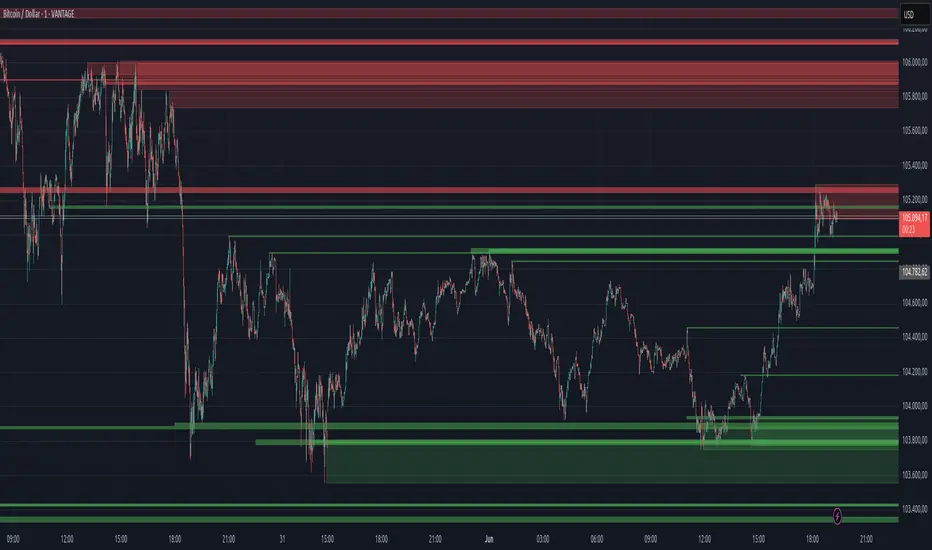
Support and Resistance MTFSupport and Resistance MTF
Support and Resistance MTF is a powerful tool that automatically detects and visualizes key support and resistance levels based on pivot highs and lows, using a higher timeframe of your choice. It is designed for traders who focus on price action and market structure, and want an adaptive, clean, and customizable indicator that helps identify important market zones.
The script uses configurable pivot logic to identify levels, with user-defined parameters for pivot strength and timeframe. Once a support or resistance level is detected, it is displayed on the chart either as a horizontal line, a shaded box, or both, depending on your display settings. You can fully customize the visual appearance including color, transparency, and line thickness. Levels are automatically extended into the future, and optionally into the past, to give better context.
Each level is monitored for breakout behavior. If price breaks through a level, it can change its role — a former resistance may become support, and vice versa. After a certain number of breakouts (which you define), the level is considered invalid and is automatically removed from the chart. This helps to maintain a clean visual layout and ensures only relevant levels are shown.
The indicator supports multi-timeframe analysis, allowing you to overlay higher-timeframe structure directly on your lower-timeframe trading chart. It is also compatible with Heikin Ashi candles internally for reference, without affecting your main chart type.
Support and Resistance MTF is ideal for traders looking to align intraday setups with higher-timeframe zones, manage risk around structural levels, or simply highlight market turning points in a clear and automated way. Built with Pine Script v5 and optimized for performance, it is both powerful and lightweight.
⚙️ Input Parameters – Description
[Time-Frame
Defines the higher timeframe used for detecting support and resistance levels. For example, you can set this to 1h, 4h, or D to visualize significant levels from a broader market perspective on a lower-timeframe chart.
Left / Right (Pivot Left / Pivot Right)
These parameters control the sensitivity of the pivot detection. A pivot high/low is confirmed if it is higher/lower than the defined number of candles to its left and right. Higher values reduce noise but may miss smaller turning points.
Extend Left
When enabled, the drawn levels (lines and/or boxes) are extended to the left side of the chart, allowing you to see the historical alignment of these levels.
Max Breaks Before Delete
Defines how many times a level can be broken by price before it is removed from the chart. This helps to avoid clutter from outdated or invalidated levels and keeps your chart relevant to current price action.
Draw Lines Only
If enabled, the indicator will draw only horizontal lines for support and resistance zones, omitting the colored background boxes. Useful for a cleaner chart appearance.
Line Width Broken Level
Sets the thickness of the support/resistance lines. Thicker lines can emphasize key levels, especially after a breakout.
Transparency Boxes
Controls the transparency (0–100) of the background boxes representing the zones. A higher value makes the boxes more transparent, lower values make them more opaque.
Transparency Lines
Controls the transparency (0–100) of the horizontal support and resistance lines. This allows for visual fine-tuning based on chart background and personal preference.
Support (Color, Group: Display)
Lets you choose the color used for support zones and lines. By default, it's green, but you can change it to fit your theme or visual preference.
Resistance (Color, Group: Display)
Defines the color for resistance zones and lines. The default is red, but it can be customized freely.
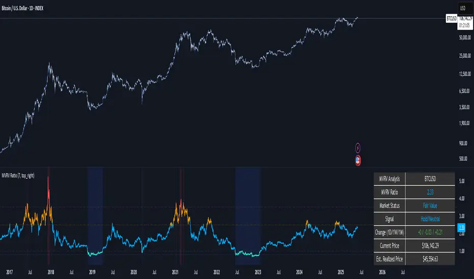
MVRV Ratio [Alpha Extract]The MVRV Ratio Indicator provides valuable insights into Bitcoin market cycles by tracking the relationship between market value and realized value. This powerful on-chain metric helps traders identify potential market tops and bottoms, offering clear buy and sell signals based on historical patterns of Bitcoin valuation.
🔶 CALCULATION The indicator processes MVRV ratio data through several analytical methods:
Raw MVRV Data: Collects MVRV data directly from INTOTHEBLOCK for Bitcoin
Optional Smoothing: Applies simple moving average (SMA) to reduce noise
Status Classification: Categorizes market conditions into four distinct states
Signal Generation: Produces trading signals based on MVRV thresholds
Price Estimation: Calculates estimated realized price (Current price / MVRV ratio)
Historical Context: Compares current values to historical extremes
Formula:
MVRV Ratio = Market Value / Realized Value
Smoothed MVRV = SMA(MVRV Ratio, Smoothing Length)
Estimated Realized Price = Current Price / MVRV Ratio
Distance to Top = ((3.5 / MVRV Ratio) - 1) * 100
Distance to Bottom = ((MVRV Ratio / 0.8) - 1) * 100
🔶 DETAILS Visual Features:
MVRV Plot: Color-coded line showing current MVRV value (red for overvalued, orange for moderately overvalued, blue for fair value, teal for undervalued)
Reference Levels: Horizontal lines indicating key MVRV thresholds (3.5, 2.5, 1.0, 0.8)
Zone Highlighting: Background color changes to highlight extreme market conditions (red for potentially overvalued, blue for potentially undervalued)
Information Table: Comprehensive dashboard showing current MVRV value, market status, trading signal, price information, and historical context
Interpretation:
MVRV ≥ 3.5: Potential market top, strong sell signal
MVRV ≥ 2.5: Overvalued market, consider selling
MVRV 1.5-2.5: Neutral market conditions
MVRV 1.0-1.5: Fair value, consider buying
MVRV < 1.0: Potential market bottom, strong buy signal
🔶 EXAMPLES
Market Top Identification: When MVRV ratio exceeds 3.5, the indicator signals potential market tops, highlighting periods where Bitcoin may be significantly overvalued.
Example: During bull market peaks, MVRV exceeding 3.5 has historically preceded major corrections, helping traders time their exits.
Bottom Detection: MVRV values below 1.0, especially approaching 0.8, have historically marked excellent buying opportunities.
Example: During bear market bottoms, MVRV falling below 1.0 has identified the most profitable entry points for long-term Bitcoin accumulation.
Tracking Market Cycles: The indicator provides a clear visualization of Bitcoin's market cycles from undervalued to overvalued states.
Example: Following the progression of MVRV from below 1.0 through fair value and eventually to overvalued territory helps traders position themselves appropriately throughout Bitcoin's market cycle.
Realized Price Support: The estimated realized price often acts as a significant
support/resistance level during market transitions.
Example: During corrections, price often finds support near the realized price level calculated by the indicator, providing potential entry points.
🔶 SETTINGS
Customization Options:
Smoothing: Toggle smoothing option and adjust smoothing length (1-50)
Table Display: Show/hide the information table
Table Position: Choose between top right, top left, bottom right, or bottom left positions
Visual Elements: All plots, lines, and background highlights can be customized for color and style
The MVRV Ratio Indicator provides traders with a powerful on-chain metric to identify potential market tops and bottoms in Bitcoin. By tracking the relationship between market value and realized value, this indicator helps identify periods of overvaluation and undervaluation, offering clear buy and sell signals based on historical patterns. The comprehensive information table delivers valuable context about current market conditions, helping traders make more informed decisions about market positioning throughout Bitcoin's cyclical patterns.
LTA - Futures Contract Size CalculatorLTA - Futures Contract Size Calculator
This indicator helps futures traders calculate the potential stop-loss (SL) value for their trades with ease. Simply input your entry price, stop-loss price, and number of contracts, and the indicator will compute the ticks moved, price movement, and total SL value in USD.
Key Features:
Supports a wide range of futures contracts, including:
Index Futures: E-mini S&P 500 (ES), Micro E-mini S&P 500 (MES), E-mini Nasdaq-100 (NQ), Micro E-mini Nasdaq-100 (MNQ)
Commodity Futures: Crude Oil (CL), Gold (GC), Micro Gold (MGC), Silver (SI), Micro Silver (SIL), Platinum (PL), Micro Platinum (MPL), Natural Gas (NG), Micro Natural Gas (MNG)
Bond Futures: 30-Year T-Bond (ZB)
Currency Futures: Euro FX (6E), Japanese Yen (6J), Australian Dollar (6A), British Pound (6B), Canadian Dollar (6C), Swiss Franc (6S), New Zealand Dollar (6N)
Displays key metrics in a clean table (bottom-right corner):
Instrument, Entry Price, Stop-Loss Price, Number of Contracts, Tick Size, Ticks Moved, Price Movement, and Total SL Value.
Automatically calculates based on the selected instrument’s tick size and tick value.
User-friendly interface with a dark theme for better visibility.
How to Use:
Add the indicator to your chart.
Select your instrument from the dropdown (ensure it matches your chart’s symbol, e.g., "NG1!" for NATURAL GAS (NG)).
Input your Entry Price, Stop-Loss Price, and Number of Contracts.
View the results in the table, including the Total SL Value in USD.
Ideal For:
Futures traders looking to quickly assess stop-loss risk.
Beginners and pros trading indices, commodities, bonds, or currencies.
Note: Ensure your chart symbol matches the selected instrument for accurate calculations. For best results, test with a few contracts and price levels to confirm the output.
This description is tailored for TradingView’s audience, providing a clear overview of the indicator’s functionality, supported instruments, and usage instructions. It also includes a note to help users avoid common pitfalls (e.g., mismatched symbols). If you’d like to adjust the tone, add more details, or include specific TradingView tags (e.g., , ), let me know!

Ultimate Scalping Tool[BullByte]Overview
The Ultimate Scalping Tool is an open-source TradingView indicator built for scalpers and short-term traders released under the Mozilla Public License 2.0. It uses a custom Quantum Flux Candle (QFC) oscillator to combine multiple market forces into one visual signal. In plain terms, the script reads momentum, trend strength, volatility, and volume together and plots a special “candlestick” each bar (the QFC) that reflects the overall market bias. This unified view makes it easier to spot entries and exits: the tool labels signals as Strong Buy/Sell, Pullback (a brief retracement in a trend), Early Entry, or Exit Warning . It also provides color-coded alerts and a small dashboard of metrics. In practice, traders see green/red oscillator bars and symbols on the chart when conditions align, helping them scalp or trend-follow without reading multiple separate indicators.
Core Components
Quantum Flux Candle (QFC) Construction
The QFC is the heart of the indicator. Rather than using raw price, it creates a candlestick-like bar from the underlying oscillator values. Each QFC bar has an “open,” “high/low,” and “close” derived from calculated momentum and volatility inputs for that period . In effect, this turns the oscillator into intuitive candle patterns so traders can recognize momentum shifts visually. (For comparison, note that Heikin-Ashi candles “have a smoother look because take an average of the movement”. The QFC instead represents exact oscillator readings, so it reflects true momentum changes without hiding price action.) Colors of QFC bars change dynamically (e.g. green for bullish momentum, red for bearish) to highlight shifts. This is the first open-source QFC oscillator that dynamically weights four non-correlated indicators with moving thresholds, which makes it a unique indicator on its own.
Oscillator Normalization & Adaptive Weights
The script normalizes its oscillator to a fixed scale (for example, a 0–100 range much like the RSI) so that various inputs can be compared fairly. It then applies adaptive weighting: the relative influence of trend, momentum, volatility or volume signals is automatically adjusted based on current market conditions. For instance, in very volatile markets the script might weight volatility more heavily, or in a strong trend it might give extra weight to trend direction. Normalizing data and adjusting weights helps keep the QFC sensitive but stable (normalization ensures all inputs fit a common scale).
Trend/Momentum/Volume/Volatility Fusion
Unlike a typical single-factor oscillator, the QFC oscillator fuses four aspects at once. It may compute, for example, a trend indicator (such as an ADX or moving average slope), a momentum measure (like RSI or Rate-of-Change), a volume-based pressure (similar to MFI/OBV), and a volatility measure (like ATR) . These different values are combined into one composite oscillator. This “multi-dimensional” approach follows best practices of using non-correlated indicators (trend, momentum, volume, volatility) for confirmation. By encoding all these signals in one line, a high QFC reading means that trend, momentum, and volume are all aligned, whereas a neutral reading might mean mixed conditions. This gives traders a comprehensive picture of market strength.
Signal Classification
The script interprets the QFC oscillator to label trades. For example:
• Strong Buy/Sell : Triggered when the oscillator crosses a high-confidence threshold (e.g. breaks clearly above zero with strong slope), indicating a well-confirmed move. This is like seeing a big green/red QFC candle aligned with the trend.
• Pullbacks : Identified when the trend is up but momentum dips briefly. A Pullback Buy appears if the overall trend is bullish but the oscillator has a short retracement – a typical buying opportunity in an uptrend. (A pullback is “a brief decline or pause in a generally upward price trend”.)
• Early Buy/Sell : Marks an initial swing in the oscillator suggesting a possible new trend, before it is fully confirmed. It’s a hint of momentum building (an early-warning signal), not as strong as the confirmed “Strong” signal.
• Exit Warnings : Issued when momentum peaks or reverses. For instance, if the QFC bars reach a high and start turning red/green opposite, the indicator warns that the move may be ending. In other words, a Momentum Peak is the point of maximum strength after which weakness may follow.
These categories correspond to typical trading concepts: Pullback (temporary reversal in an uptrend), Early Buy (an initial bullish cross), Strong Buy (confirmed bullish momentum), and Momentum Peak (peak oscillator value suggesting exhaustion).
Filters (DI Reversal, Dynamic Thresholds, HTF EMA/ADX)
Extra filters help avoid bad trades. A DI Reversal filter uses the +DI/–DI lines (from the ADX system) to require that the trend direction confirms the signal . For example, it might ignore a buy signal if the +DI is still below –DI. Dynamic Thresholds adjust signal levels on-the-fly: rather than fixed “overbought” lines, they move with volatility so signals happen under appropriate market stress. An optional High-Timeframe EMA or ADX filter adds a check against a larger timeframe trend: for instance, only taking a trade if price is above the weekly EMA or if weekly ADX shows a strong trend. (Notably, the ADX is “a technical indicator used by traders to determine the strength of a price trend”, so requiring a high-timeframe ADX avoids trading against the bigger trend.)
Dashboard Metrics & Color Logic
The Dashboard in the Ultimate Scalping Tool (UST) serves as a centralized information hub, providing traders with real-time insights into market conditions, trend strength, momentum, volume pressure, and trade signals. It is highly customizable, allowing users to adjust its appearance and content based on their preferences.
1. Dashboard Layout & Customization
Short vs. Extended Mode : Users can toggle between a compact view (9 rows) and an extended view (13 rows) via the `Short Dashboard` input.
Text Size Options : The dashboard supports three text sizes— Tiny, Small, and Normal —adjustable via the `Dashboard Text Size` input.
Positioning : The dashboard is positioned in the top-right corner by default but can be moved if modified in the script.
2. Key Metrics Displayed
The dashboard presents critical trading metrics in a structured table format:
Trend (TF) : Indicates the current trend direction (Strong Bullish, Moderate Bullish, Sideways, Moderate Bearish, Strong Bearish) based on normalized trend strength (normTrend) .
Momentum (TF) : Displays momentum status (Strong Bullish/Bearish or Neutral) derived from the oscillator's position relative to dynamic thresholds.
Volume (CMF) : Shows buying/selling pressure levels (Very High Buying, High Selling, Neutral, etc.) based on the Chaikin Money Flow (CMF) indicator.
Basic & Advanced Signals:
Basic Signal : Provides simple trade signals (Strong Buy, Strong Sell, Pullback Buy, Pullback Sell, No Trade).
Advanced Signal : Offers nuanced signals (Early Buy/Sell, Momentum Peak, Weakening Momentum, etc.) with color-coded alerts.
RSI : Displays the Relative Strength Index (RSI) value, colored based on overbought (>70), oversold (<30), or neutral conditions.
HTF Filter : Indicates the higher timeframe trend status (Bullish, Bearish, Neutral) when using the Leading HTF Filter.
VWAP : Shows the V olume-Weighted Average Price and whether the current price is above (bullish) or below (bearish) it.
ADX : Displays the Average Directional Index (ADX) value, with color highlighting whether it is rising (green) or falling (red).
Market Mode : Shows the selected market type (Crypto, Stocks, Options, Forex, Custom).
Regime : Indicates volatility conditions (High, Low, Moderate) based on the **ATR ratio**.
3. Filters Status Panel
A secondary panel displays the status of active filters, helping traders quickly assess which conditions are influencing signals:
- DI Reversal Filter: On/Off (confirms reversals before generating signals).
- Dynamic Thresholds: On/Off (adjusts buy/sell thresholds based on volatility).
- Adaptive Weighting: On/Off (auto-adjusts oscillator weights for trend/momentum/volatility).
- Early Signal: On/Off (enables early momentum-based signals).
- Leading HTF Filter: On/Off (applies higher timeframe trend confirmation).
4. Visual Enhancements
Color-Coded Cells : Each metric is color-coded (green for bullish, red for bearish, gray for neutral) for quick interpretation.
Dynamic Background : The dashboard background adapts to market conditions (bullish/bearish/neutral) based on ADX and DI trends.
Customizable Reference Lines : Users can enable/disable fixed reference lines for the oscillator.
How It(QFC) Differs from Traditional Indicators
Quantum Flux Candle (QFC) Versus Heikin-Ashi
Heikin-Ashi candles smooth price by averaging (HA’s open/close use averages) so they show trend clearly but hide true price (the current HA bar’s close is not the real price). QFC candles are different: they are oscillator values, not price averages . A Heikin-Ashi chart “has a smoother look because it is essentially taking an average of the movement”, which can cause lag. The QFC instead shows the raw combined momentum each bar, allowing faster recognition of shifts. In short, HA is a smoothed price chart; QFC is a momentum-based chart.
Versus Standard Oscillators
Common oscillators like RSI or MACD use fixed formulas on price (or price+volume). For example, RSI “compares gains and losses and normalizes this value on a scale from 0 to 100”, reflecting pure price momentum. MFI is similar but adds volume. These indicators each show one dimension: momentum or volume. The Ultimate Scalping Tool’s QFC goes further by integrating trend strength and volatility too. In practice, this means a move that looks strong on RSI might be downplayed by low volume or weak trend in QFC. As one source notes, using multiple non-correlated indicators (trend, momentum, volume, volatility) provides a more complete market picture. The QFC’s multi-factor fusion is unique – it is effectively a multi-dimensional oscillator rather than a traditional single-input one.
Signal Style
Traditional oscillators often use crossovers (RSI crossing 50) or fixed zones (MACD above zero) for signals. The Ultimate Scalping Tool’s signals are custom-classified: it explicitly labels pullbacks, early entries, and strong moves. These terms go beyond a typical indicator’s generic “buy”/“sell.” In other words, it packages a strategy around the oscillator, which traders can backtest or observe without reading code.
Key Term Definitions
• Pullback : A short-term dip or consolidation in an uptrend. In this script, a Pullback Buy appears when price is generally rising but shows a brief retracement. (As defined by Investopedia, a pullback is “a brief decline or pause in a generally upward price trend”.)
• Early Buy/Sell : An initial or tentative entry signal. It means the oscillator first starts turning positive (or negative) before a full trend has developed. It’s an early indication that a trend might be starting.
• Strong Buy/Sell : A confident entry signal when multiple conditions align. This label is used when momentum is already strong and confirmed by trend/volume filters, offering a higher-probability trade.
• Momentum Peak : The point where bullish (or bearish) momentum reaches its maximum before weakening. When the oscillator value stops rising (or falling) and begins to reverse, the script flags it as a peak – signaling that the current move could be overextended.
What is the Flux MA?
The Flux MA (Moving Average) is an Exponential Moving Average (EMA) applied to a normalized oscillator, referred to as FM . Its purpose is to smooth out the fluctuations of the oscillator, providing a clearer picture of the underlying trend direction and strength. Think of it as a dynamic baseline that the oscillator moves above or below, helping you determine whether the market is trending bullish or bearish.
How it’s calculated (Flux MA):
1.The oscillator is normalized (scaled to a range, typically between 0 and 1, using a default scale factor of 100.0).
2.An EMA is applied to this normalized value (FM) over a user-defined period (default is 10 periods).
3.The result is rescaled back to the oscillator’s original range for plotting.
Why it matters : The Flux MA acts like a support or resistance level for the oscillator, making it easier to spot trend shifts.
Color of the Flux Candle
The Quantum Flux Candle visualizes the normalized oscillator (FM) as candlesticks, with colors that indicate specific market conditions based on the relationship between the FM and the Flux MA. Here’s what each color means:
• Green : The FM is above the Flux MA, signaling bullish momentum. This suggests the market is trending upward.
• Red : The FM is below the Flux MA, signaling bearish momentum. This suggests the market is trending downward.
• Yellow : Indicates strong buy conditions (e.g., a "Strong Buy" signal combined with a positive trend). This is a high-confidence signal to go long.
• Purple : Indicates strong sell conditions (e.g., a "Strong Sell" signal combined with a negative trend). This is a high-confidence signal to go short.
The candle mode shows the oscillator’s open, high, low, and close values for each period, similar to price candlesticks, but it’s the color that provides the quick visual cue for trading decisions.
How to Trade the Flux MA with Respect to the Candle
Trading with the Flux MA and Quantum Flux Candle involves using the MA as a trend indicator and the candle colors as entry and exit signals. Here’s a step-by-step guide:
1. Identify the Trend Direction
• Bullish Trend : The Flux Candle is green and positioned above the Flux MA. This indicates upward momentum.
• Bearish Trend : The Flux Candle is red and positioned below the Flux MA. This indicates downward momentum.
The Flux MA serves as the reference line—candles above it suggest buying pressure, while candles below it suggest selling pressure.
2. Interpret Candle Colors for Trade Signals
• Green Candle : General bullish momentum. Consider entering or holding a long position.
• Red Candle : General bearish momentum. Consider entering or holding a short position.
• Yellow Candle : A strong buy signal. This is an ideal time to enter a long trade.
• Purple Candle : A strong sell signal. This is an ideal time to enter a short trade.
3. Enter Trades Based on Crossovers and Colors
• Long Entry : Enter a buy position when the Flux Candle turns green and crosses above the Flux MA. If it turns yellow, this is an even stronger signal to go long.
• Short Entry : Enter a sell position when the Flux Candle turns red and crosses below the Flux MA. If it turns purple, this is an even stronger signal to go short.
4. Exit Trades
• Exit Long : Close your buy position when the Flux Candle turns red or crosses below the Flux MA, indicating the bullish trend may be reversing.
• Exit Short : Close your sell position when the Flux Candle turns green or crosses above the Flux MA, indicating the bearish trend may be reversing.
•You might also exit a long trade if the candle changes from yellow to green (weakening strong buy signal) or a short trade from purple to red (weakening strong sell signal).
5. Use Additional Confirmation
To avoid false signals, combine the Flux MA and candle signals with other indicators or dashboard metrics (e.g., trend strength, momentum, or volume pressure). For example:
•A yellow candle with a " Strong Bullish " trend and high buying volume is a robust long signal.
•A red candle with a " Moderate Bearish " trend and neutral momentum might need more confirmation before shorting.
Practical Example
Imagine you’re scalping a cryptocurrency:
• Long Trade : The Flux Candle turns yellow and is above the Flux MA, with the dashboard showing "Strong Buy" and high buying volume. You enter a long position. You exit when the candle turns red and dips below the Flux MA.
• Short Trade : The Flux Candle turns purple and crosses below the Flux MA, with a "Strong Sell" signal on the dashboard. You enter a short position. You exit when the candle turns green and crosses above the Flux MA.
Market Presets and Adaptation
This indicator is designed to work on any market with candlestick price data (stocks, crypto, forex, indices, etc.). To handle different behavior, it provides presets for major asset classes. Selecting a “Stocks,” “Crypto,” “Forex,” or “Options” preset automatically loads a set of parameter values optimized for that market . For example, a crypto preset might use a shorter lookback or higher sensitivity to account for crypto’s high volatility, while a stocks preset might use slightly longer smoothing since stocks often trend more slowly. In practice, this means the same core QFC logic applies across markets, but the thresholds and smoothing adjust so signals remain relevant for each asset type.
Usage Guidelines
• Recommended Timeframes : Optimized for 1 minute to 15 minute intraday charts. Can also be used on higher timeframes for short term swings.
• Market Types : Select “Crypto,” “Stocks,” “Forex,” or “Options” to auto tune periods, thresholds and weights. Use “Custom” to manually adjust all inputs.
• Interpreting Signals : Always confirm a signal by checking that trend, volume, and VWAP agree on the dashboard. A green “Strong Buy” arrow with green trend, green volume, and price > VWAP is highest probability.
• Adjusting Sensitivity : To reduce false signals in fast markets, enable DI Reversal Confirmation and Dynamic Thresholds. For more frequent entries in trending environments, enable Early Entry Trigger.
• Risk Management : This tool does not plot stop loss or take profit levels. Users should define their own risk parameters based on support/resistance or volatility bands.
Background Shading
To give you an at-a-glance sense of market regime without reading numbers, the indicator automatically tints the chart background in three modes—neutral, bullish and bearish—with two levels of intensity (light vs. dark):
Neutral (Gray)
When ADX is below 20 the market is considered “no trend” or too weak to trade. The background fills with a light gray (high transparency) so you know to sit on your hands.
Bullish (Green)
As soon as ADX rises above 20 and +DI exceeds –DI, the background turns a semi-transparent green, signaling an emerging uptrend. When ADX climbs above 30 (strong trend), the green becomes more opaque—reminding you that trend-following signals (Strong Buy, Pullback) carry extra weight.
Bearish (Red)
Similarly, if –DI exceeds +DI with ADX >20, you get a light red tint for a developing downtrend, and a darker, more solid red once ADX surpasses 30.
By dynamically varying both hue (green vs. red vs. gray) and opacity (light vs. dark), the background instantly communicates trend strength and direction—so you always know whether to favor breakout-style entries (in a strong trend) or stay flat during choppy, low-ADX conditions.
The setup shown in the above chart snapshot is BTCUSD 15 min chart : Binance for reference.
Disclaimer
No indicator guarantees profits. Backtest or paper trade this tool to understand its behavior in your market. Always use proper position sizing and stop loss orders.
Good luck!
- BullByte

JPMorgan G7 Volatility IndexThe JPMorgan G7 Volatility Index: Scientific Analysis and Professional Applications
Introduction
The JPMorgan G7 Volatility Index (G7VOL) represents a sophisticated metric for monitoring currency market volatility across major developed economies. This indicator functions as an approximation of JPMorgan's proprietary volatility indices, providing traders and investors with a normalized measurement of cross-currency volatility conditions (Clark, 2019).
Theoretical Foundation
Currency volatility is fundamentally defined as "the statistical measure of the dispersion of returns for a given security or market index" (Hull, 2018, p.127). In the context of G7 currencies, this volatility measurement becomes particularly significant due to the economic importance of these nations, which collectively represent more than 50% of global nominal GDP (IMF, 2022).
According to Menkhoff et al. (2012, p.685), "currency volatility serves as a global risk factor that affects expected returns across different asset classes." This finding underscores the importance of monitoring G7 currency volatility as a proxy for global financial conditions.
Methodology
The G7VOL indicator employs a multi-step calculation process:
Individual volatility calculation for seven major currency pairs using standard deviation normalized by price (Lo, 2002)
- Weighted-average combination of these volatilities to form a composite index
- Normalization against historical bands to create a standardized scale
- Visual representation through dynamic coloring that reflects current market conditions
The mathematical foundation follows the volatility calculation methodology proposed by Bollerslev et al. (2018):
Volatility = σ(returns) / price × 100
Where σ represents standard deviation calculated over a specified timeframe, typically 20 periods as recommended by the Bank for International Settlements (BIS, 2020).
Professional Applications
Professional traders and institutional investors employ the G7VOL indicator in several key ways:
1. Risk Management Signaling
According to research by Adrian and Brunnermeier (2016), elevated currency volatility often precedes broader market stress. When the G7VOL breaches its high volatility threshold (typically 1.5 times the 100-period average), portfolio managers frequently reduce risk exposure across asset classes. As noted by Borio (2019, p.17), "currency volatility spikes have historically preceded equity market corrections by 2-7 trading days."
2. Counter-Cyclical Investment Strategy
Low G7 volatility periods (readings below the lower band) tend to coincide with what Shin (2017) describes as "risk-on" environments. Professional investors often use these signals to increase allocations to higher-beta assets and emerging markets. Campbell et al. (2021) found that G7 volatility in the lowest quintile historically preceded emerging market outperformance by an average of 3.7% over subsequent quarters.
3. Regime Identification
The normalized volatility framework enables identification of distinct market regimes:
- Readings above 1.0: Crisis/high volatility regime
- Readings between -0.5 and 0.5: Normal volatility regime
- Readings below -1.0: Unusually calm markets
According to Rey (2015), these regimes have significant implications for global monetary policy transmission mechanisms and cross-border capital flows.
Interpretation and Trading Applications
G7 currency volatility serves as a barometer for global financial conditions due to these currencies' centrality in international trade and reserve status. As noted by Gagnon and Ihrig (2021, p.423), "G7 currency volatility captures both trade-related uncertainty and broader financial market risk appetites."
Professional traders apply this indicator in multiple contexts:
- Leading indicator: Research from the Federal Reserve Board (Powell, 2020) suggests G7 volatility often leads VIX movements by 1-3 days, providing advance warning of broader market volatility.
- Correlation shifts: During periods of elevated G7 volatility, cross-asset correlations typically increase what Brunnermeier and Pedersen (2009) term "correlation breakdown during stress periods." This phenomenon informs portfolio diversification strategies.
- Carry trade timing: Currency carry strategies perform best during low volatility regimes as documented by Lustig et al. (2011). The G7VOL indicator provides objective thresholds for initiating or exiting such positions.
References
Adrian, T. and Brunnermeier, M.K. (2016) 'CoVaR', American Economic Review, 106(7), pp.1705-1741.
Bank for International Settlements (2020) Monitoring Volatility in Foreign Exchange Markets. BIS Quarterly Review, December 2020.
Bollerslev, T., Patton, A.J. and Quaedvlieg, R. (2018) 'Modeling and forecasting (un)reliable realized volatilities', Journal of Econometrics, 204(1), pp.112-130.
Borio, C. (2019) 'Monetary policy in the grip of a pincer movement', BIS Working Papers, No. 706.
Brunnermeier, M.K. and Pedersen, L.H. (2009) 'Market liquidity and funding liquidity', Review of Financial Studies, 22(6), pp.2201-2238.
Campbell, J.Y., Sunderam, A. and Viceira, L.M. (2021) 'Inflation Bets or Deflation Hedges? The Changing Risks of Nominal Bonds', Critical Finance Review, 10(2), pp.303-336.
Clark, J. (2019) 'Currency Volatility and Macro Fundamentals', JPMorgan Global FX Research Quarterly, Fall 2019.
Gagnon, J.E. and Ihrig, J. (2021) 'What drives foreign exchange markets?', International Finance, 24(3), pp.414-428.
Hull, J.C. (2018) Options, Futures, and Other Derivatives. 10th edn. London: Pearson.
International Monetary Fund (2022) World Economic Outlook Database. Washington, DC: IMF.
Lo, A.W. (2002) 'The statistics of Sharpe ratios', Financial Analysts Journal, 58(4), pp.36-52.
Lustig, H., Roussanov, N. and Verdelhan, A. (2011) 'Common risk factors in currency markets', Review of Financial Studies, 24(11), pp.3731-3777.
Menkhoff, L., Sarno, L., Schmeling, M. and Schrimpf, A. (2012) 'Carry trades and global foreign exchange volatility', Journal of Finance, 67(2), pp.681-718.
Powell, J. (2020) Monetary Policy and Price Stability. Speech at Jackson Hole Economic Symposium, August 27, 2020.
Rey, H. (2015) 'Dilemma not trilemma: The global financial cycle and monetary policy independence', NBER Working Paper No. 21162.
Shin, H.S. (2017) 'The bank/capital markets nexus goes global', Bank for International Settlements Speech, January 15, 2017.

Consecutive Candles Above/Below EMADescription:
This indicator identifies and highlights periods where the price remains consistently above or below an Exponential Moving Average (EMA) for a user-defined number of consecutive candles. It visually marks these sustained trends with background colors and labels, helping traders spot strong bullish or bearish market conditions. Ideal for trend-following strategies or identifying potential trend exhaustion points, this tool provides clear visual cues for price behavior relative to the EMA.
How It Works:
EMA Calculation: The indicator calculates an EMA based on the user-specified period (default: 100). The EMA is plotted as a blue line on the chart for reference.
Consecutive Candle Tracking: It counts how many consecutive candles close above or below the EMA:
If a candle closes below the EMA, the "below" counter increments; any candle closing above resets it to zero.
If a candle closes above the EMA, the "above" counter increments; any candle closing below resets it to zero.
Highlighting Trends: When the number of consecutive candles above or below the EMA meets or exceeds the user-defined threshold (default: 200 candles):
A translucent red background highlights periods where the price has been below the EMA.
A translucent green background highlights periods where the price has been above the EMA.
Labeling: When the required number of consecutive candles is first reached:
A red downward arrow label with the text "↓ Below" appears for below-EMA streaks.
A green upward arrow label with the text "↑ Above" appears for above-EMA streaks.
Usage:
Trend Confirmation: Use the highlights and labels to confirm strong trends. For example, 200 candles above the EMA may indicate a robust uptrend.
Reversal Signals: Prolonged streaks (e.g., 200+ candles) might suggest overextension, potentially signaling reversals.
Customization: Adjust the EMA period to make it faster or slower, and modify the candle count to make the indicator more or less sensitive to trends.
Settings:
EMA Length: Set the period for the EMA calculation (default: 100).
Candles Count: Define the minimum number of consecutive candles required to trigger highlights and labels (default: 200).
Visuals:
Blue EMA line for tracking the moving average.
Red background for sustained below-EMA periods.
Green background for sustained above-EMA periods.
Labeled arrows to mark when the streak threshold is met.
This indicator is a powerful tool for traders looking to visualize and capitalize on persistent price trends relative to the EMA, with clear, customizable signals for market analysis.
Explain EMA calculation
Other trend indicators
Make description shorter
%MAThis indicator is designed to plot a Simple Moving Average (SMA) along with customizable upper and lower bands (% up/down) on a TradingView chart. Here's a brief but thorough explanation of its functionality:
TL;DR: This script shows percentages above and below customizable moving average timeframes & legnths. It's unique in the sense that it isn't on a separate pane & gives visual clarity against the price in real time HLOC.
1. Main SMA Plot
The script calculates a Simple Moving Average (SMA) based on user-defined inputs:
Timeframe: E.g., daily ("Daily") by default.
Length: E.g., 50 periods by default.
Color: Customizable by the user.
This SMA acts as the central reference line and can be toggled on or off using a "Show" option.
2. Upper and Lower Bands
The script generates two upper bands and two lower bands around the main SMA.
Each band is derived from an SMA (calculated similarly to the main SMA) and offset by a percentage:
Upper Bands: SMA × (1 + distance percentage / 100), e.g., SMA × 1.05 for a 5% offset.
Lower Bands: SMA × (1 - distance percentage / 100), e.g., SMA × 0.95 for a 5% offset.
These bands can indicate potential support, resistance, or volatility ranges.
3. Customization
Users can independently configure:
Visibility: Toggle each band and the main SMA on or off.
Timeframe: Set the timeframe for each SMA calculation.
Length: Define the SMA period.
Distance Percentage: Adjust the offset for each band.
Color: Choose colors for all plotted lines.
This flexibility allows tailored analysis for different trading strategies or timeframes.
4. Plotting
The main SMA and each band are plotted using TradingView’s plot function, but only if their respective "Show" options are enabled.
Lines are displayed with user-specified colors and styles (e.g., the main SMA has a linewidth of 2).
Purpose
This script provides a versatile tool for technical analysis, enabling traders to visualize an SMA with percentage-based bands to identify key price levels or ranges, such as support/resistance, volatility zones, and trends, with extensive customization options.

Pulse DPO with Z-Score📌 Pulse DPO with Z-Score — Indicator Description (English)
The Pulse DPO (Detrended Price Oscillator) helps identify major market cycle tops and bottoms by removing long-term trends and focusing on shorter-term price cycles.
This enhanced version includes:
A normalized oscillator (0–100) based on recent price deviations.
A smoothed signal to reduce noise.
A Z-Score transformation, scaling the output to a range from –3 to +3, where:
–3 represents extreme oversold conditions (former normalized value = 100),
+3 represents extreme overbought conditions (former normalized value = 1).
🔍 How it works:
The indicator subtracts a delayed moving average from price to isolate short-term cycles (DPO logic).
It then normalizes the oscillator within a lookback window.
Finally, it converts this to a Z-Score scale for easier interpretation of extremes.
🟢 Suggested Usage:
Consider Long entries or Short exits when Z-Score reaches –2 to –3 (deep oversold).
Consider Short entries or Long exits when Z-Score reaches +2 to +3 (deep overbought).
Use in combination with other signals for higher-confidence setups.
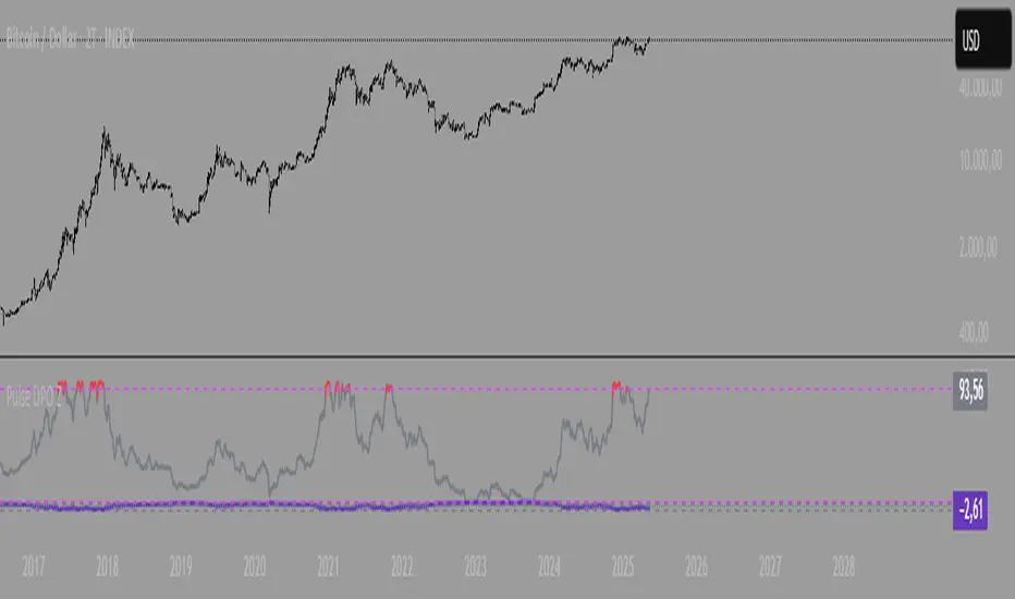
Hurst Exponent Oscillator [PhenLabs]📊 Hurst Exponent Oscillator -
Version: PineScript™ v5
📌 Description
The Hurst Exponent Oscillator (HEO) by PhenLabs is a powerful tool developed for traders who want to distinguish between trending, mean-reverting, and random market behaviors with clarity and precision. By estimating the Hurst Exponent—a statistical measure of long-term memory in financial time series—this indicator helps users make sense of underlying market dynamics that are often not visible through traditional moving averages or oscillators.
Traders can quickly know if the market is likely to continue its current direction (trending), revert to the mean, or behave randomly, allowing for more strategic timing of entries and exits. With customizable smoothing and clear visual cues, the HEO enhances decision-making in a wide range of trading environments.
🚀 Points of Innovation
Integrates advanced Hurst Exponent calculation via Rescaled Range (R/S) analysis, providing unique market character insights.
Offers real-time visual cues for trending, mean-reverting, or random price action zones.
User-controllable EMA smoothing reduces noise for clearer interpretation.
Dynamic coloring and fill for immediate visual categorization of market regime.
Configurable visual thresholds for critical Hurst levels (e.g., 0.4, 0.5, 0.6).
Fully customizable appearance settings to fit different charting preferences.
🔧 Core Components
Log Returns Calculation: Computes log returns of the selected price source to feed into the Hurst calculation, ensuring robust and scale-independent analysis.
Rescaled Range (R/S) Analysis: Assesses the dispersion and cumulative deviation over a rolling window, forming the core statistical basis for the Hurst exponent estimate.
Smoothing Engine: Applies Exponential Moving Average (EMA) smoothing to the raw Hurst value for enhanced clarity.
Dynamic Rolling Windows: Utilizes arrays to maintain efficient, real-time calculations over user-defined lengths.
Adaptive Color Logic: Assigns different highlight and fill colors based on the current Hurst value zone.
🔥 Key Features
Visually differentiates between trending, mean-reverting, and random market modes.
User-adjustable lookback and smoothing periods for tailored sensitivity.
Distinct fill and line styles for each regime to avoid ambiguity.
On-chart reference lines for strong trending and mean-reverting thresholds.
Works with any price series (close, open, HL2, etc.) for versatile application.
🎨 Visualization
Hurst Exponent Curve: Primary plotted line (smoothed if EMA is used) reflects the ongoing estimate of the Hurst exponent.
Colored Zone Filling: The area between the Hurst line and the 0.5 reference line is filled, with color and opacity dynamically indicating the current market regime.
Reference Lines: Dash/dot lines mark standard Hurst thresholds (0.4, 0.5, 0.6) to contextualize the current regime.
All visual elements can be customized for thickness, color intensity, and opacity for user preference.
📖 Usage Guidelines
Data Settings
Hurst Calculation Length
Default: 100
Range: 10-300
Description: Number of bars used in Hurst calculation; higher values mean longer-term analysis, lower values for quicker reaction.
Data Source
Default: close
Description: Select which data series to analyze (e.g., Close, Open, HL2).
Smoothing Length (EMA)
Default: 5
Range: 1-50
Description: Length for smoothing the Hurst value; higher settings yield smoother but less responsive results.
Style Settings
Trending Color (Hurst > 0.5)
Default: Blue tone
Description: Color used when trending regime is detected.
Mean-Reverting Color (Hurst < 0.5)
Default: Orange tone
Description: Color used when mean-reverting regime is detected.
Neutral/Random Color
Default: Soft blue
Description: Color when market behavior is indeterminate or shifting.
Fill Opacity
Default: 70-80
Range: 0-100
Description: Transparency of area fills—higher opacity for stronger visual effect.
Line Width
Default: 2
Range: 1-5
Description: Thickness of the main indicator curve.
✅ Best Use Cases
Identifying if a market is regime-shifting from trending to mean-reverting (or vice versa).
Filtering signals in automated or systematic trading strategies.
Spotting periods of randomness where trading signals should be deprioritized.
Enhancing mean-reversion or trend-following models with regime-awareness.
⚠️ Limitations
Not predictive: Reflects current and recent market state, not future direction.
Sensitive to input parameters—overfitting may occur if settings are changed too frequently.
Smoothing can introduce lag in regime recognition.
May not work optimally in markets with structural breaks or extreme volatility.
💡 What Makes This Unique
Employs advanced statistical market analysis (Hurst exponent) rarely found in standard toolkits.
Offers immediate regime visualization through smart dynamic coloring and zone fills.
🔬 How It Works
Rolling Log Return Calculation:
Each new price creates a log return, forming the basis for robust, non-linear analysis. This ensures all price differences are treated proportionally.
Rescaled Range Analysis:
A rolling window maintains cumulative deviations and computes the statistical “range” (max-min of deviations). This is compared against the standard deviation to estimate “memory”.
Exponent Calculation & Smoothing:
The raw Hurst value is translated from the log of the rescaled range ratio, and then optionally smoothed via EMA to dampen noise and false signals.
Regime Detection Logic:
The smoothed value is checked against 0.5. Values above = trending; below = mean-reverting; near 0.5 = random. These control plot/fill color and zone display.
💡 Note:
Use longer calculation lengths for major market character study, and shorter ones for tactical, short-term adaptation. Smoothing balances noise vs. lag—find a best fit for your trading style. Always combine regime awareness with broader technical/fundamental context for best results.
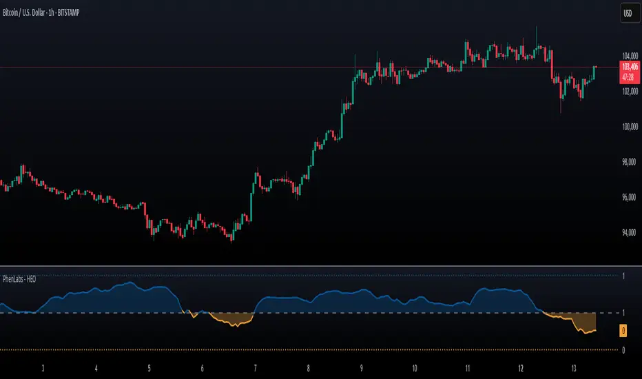
Aroon Buy & Sell (Custom TFs)Here's a detailed explanation of your Pine Script titled "Aroon Buy & Sell (Custom TFs)":
🧠 Strategy Overview:
This script generates buy and sell signals using the Aroon indicator across two different timeframes:
* One for detecting the primary trend (Trend Timeframe)
* One for confirming precise entry signals (Signal Confirmation Timeframe)
📊 Key Components:
1. User Inputs
* trendTF: The timeframe used to determine overall trend direction (e.g., 5-minute).
* signalTF: The faster timeframe for confirming trade signals (e.g., 1-minute).
* aroonLength: Lookback period for the Aroon calculation (default 14).
* cooldownPeriod: Number of bars to wait before allowing a new signal.
2. Aroon Calculation Function
Calculates Aroon Up and Aroon Down values using the number of bars since the highest high and lowest low.
3. Multi-Timeframe Aroon Values
Uses request.security to compute Aroon values on both trendTF and signalTF.
4. Trend Detection
* A bullish trend is defined when Aroon Up crosses above Aroon Down on the trend timeframe.
* A bearish trend is defined when Aroon Down crosses above Aroon Up.
5. Signal Logic
* Buy Signal: When the overall trend is bullish and Aroon Down = 100 on the signal timeframe.
* Sell Signal: When the trend is bearish and Aroon Up = 100 on the signal timeframe.
6. Cooldown Mechanism
Prevents back-to-back signals by enforcing a cooldown (e.g., 20 bars) after each buy/sell.
7. Signal Plotting & Alerts
Plots buy/sell signals directly on the chart and supports alerts for automation.
📈 Visual Output:
* BUY label below the bar when buy conditions are met.
* SELL label above the bar when sell conditions are met.
🔔 Alerts:
Two alertconditions are defined to trigger alerts whenever a buy or sell signal occurs.
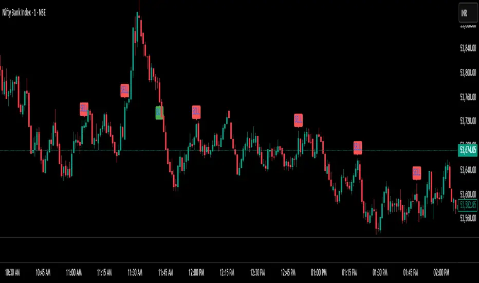
CRT Finder (WanHakimFX)📈 Liquidity Grab Indicator with MTF Confluence & Alerts
🔍 Overview:
The Liquidity Grab Indicator is designed to detect precise moments when price sweeps liquidity — either by wicking below recent lows (bullish LQH) or above recent highs (bearish LQL) — followed by a clear rejection. It combines this logic with multi-timeframe confirmation and trend filters, making it a powerful tool for identifying high-probability reversal setups.
⚙️ How It Works:
✅ Liquidity Sweep Logic (LQH / LQL)
Bullish (LQH):
Current candle wicks below the previous low
Closes above the previous candle body
Confirms potential bullish reversal
Bearish (LQL):
Current candle wicks above the previous high
Closes below the previous candle body
Confirms potential bearish reversal
✅ Additional Conditions:
Must occur during London or New York sessions.
Requires trend confluence:
LQH = Price must be above SMMA 60/100/200
LQL = Price must be below SMMA 60/100/200
🧠 Multi-Timeframe Confluence:
The indicator scans for LQH/LQL sweeps across:
Daily
4H
1H
30M
15M
If a sweep occurs on any of these timeframes, an alert is triggered and a triangle marker appears on the chart for real-time visual confluence.
📊 Visual Features:
Green/Red labels for active timeframe sweeps.
Dotted wick lines to show liquidity zones from the previous candle.
Colored triangle markers for MTF sweep alerts.
🛠 Strategy Usage:
This indicator is best used as a trigger tool in a confluence-based strategy:
Use higher-timeframe MTF LQH/LQL markers for directional bias.
Wait for matching sweep on your entry timeframe (e.g., M1/M5).
Enter on confirmation candle or break of structure.
Target imbalances, FVGs, or previous highs/lows.
Risk-managed entries using sweep candle's high/low as stop.
📢 Alerts:
✅ Bullish Sweep (LQH) on any timeframe
✅ Bearish Sweep (LQL) on any timeframe

ADX Forecast [Titans_Invest]ADX Forecast
This isn’t just another ADX indicator — it’s the most powerful and complete ADX tool ever created, and without question the best ADX indicator on TradingView, possibly even the best in the world.
ADX Forecast represents a revolutionary leap in trend strength analysis, blending the timeless principles of the classic ADX with cutting-edge predictive modeling. For the first time on TradingView, you can anticipate future ADX movements using scientifically validated linear regression — a true game-changer for traders looking to stay ahead of trend shifts.
1. Real-Time ADX Forecasting
By applying least squares linear regression, ADX Forecast projects the future trajectory of the ADX with exceptional accuracy. This forecasting power enables traders to anticipate changes in trend strength before they fully unfold — a vital edge in fast-moving markets.
2. Unmatched Customization & Precision
With 26 long entry conditions and 26 short entry conditions, this indicator accounts for every possible ADX scenario. Every parameter is fully customizable, making it adaptable to any trading strategy — from scalping to swing trading to long-term investing.
3. Transparency & Advanced Visualization
Visualize internal ADX dynamics in real time with interactive tags, smart flags, and fully adjustable threshold levels. Every signal is transparent, logic-based, and engineered to fit seamlessly into professional-grade trading systems.
4. Scientific Foundation, Elite Execution
Grounded in statistical precision and machine learning principles, ADX Forecast upgrades the classic ADX from a reactive lagging tool into a forward-looking trend prediction engine. This isn’t just an indicator — it’s a scientific evolution in trend analysis.
⯁ SCIENTIFIC BASIS LINEAR REGRESSION
Linear Regression is a fundamental method of statistics and machine learning, used to model the relationship between a dependent variable y and one or more independent variables 𝑥.
The general formula for a simple linear regression is given by:
y = β₀ + β₁x + ε
β₁ = Σ((xᵢ - x̄)(yᵢ - ȳ)) / Σ((xᵢ - x̄)²)
β₀ = ȳ - β₁x̄
Where:
y = is the predicted variable (e.g. future value of RSI)
x = is the explanatory variable (e.g. time or bar index)
β0 = is the intercept (value of 𝑦 when 𝑥 = 0)
𝛽1 = is the slope of the line (rate of change)
ε = is the random error term
The goal is to estimate the coefficients 𝛽0 and 𝛽1 so as to minimize the sum of the squared errors — the so-called Random Error Method Least Squares.
⯁ LEAST SQUARES ESTIMATION
To minimize the error between predicted and observed values, we use the following formulas:
β₁ = /
β₀ = ȳ - β₁x̄
Where:
∑ = sum
x̄ = mean of x
ȳ = mean of y
x_i, y_i = individual values of the variables.
Where:
x_i and y_i are the means of the independent and dependent variables, respectively.
i ranges from 1 to n, the number of observations.
These equations guarantee the best linear unbiased estimator, according to the Gauss-Markov theorem, assuming homoscedasticity and linearity.
⯁ LINEAR REGRESSION IN MACHINE LEARNING
Linear regression is one of the cornerstones of supervised learning. Its simplicity and ability to generate accurate quantitative predictions make it essential in AI systems, predictive algorithms, time series analysis, and automated trading strategies.
By applying this model to the ADX, you are literally putting artificial intelligence at the heart of a classic indicator, bringing a new dimension to technical analysis.
⯁ VISUAL INTERPRETATION
Imagine an ADX time series like this:
Time →
ADX →
The regression line will smooth these values and extend them n periods into the future, creating a predicted trajectory based on the historical moment. This line becomes the predicted ADX, which can be crossed with the actual ADX to generate more intelligent signals.
⯁ SUMMARY OF SCIENTIFIC CONCEPTS USED
Linear Regression Models the relationship between variables using a straight line.
Least Squares Minimizes the sum of squared errors between prediction and reality.
Time Series Forecasting Estimates future values based on historical data.
Supervised Learning Trains models to predict outputs from known inputs.
Statistical Smoothing Reduces noise and reveals underlying trends.
⯁ WHY THIS INDICATOR IS REVOLUTIONARY
Scientifically-based: Based on statistical theory and mathematical inference.
Unprecedented: First public ADX with least squares predictive modeling.
Intelligent: Built with machine learning logic.
Practical: Generates forward-thinking signals.
Customizable: Flexible for any trading strategy.
⯁ CONCLUSION
By combining ADX with linear regression, this indicator allows a trader to predict market momentum, not just follow it.
ADX Forecast is not just an indicator — it is a scientific breakthrough in technical analysis technology.
⯁ Example of simple linear regression, which has one independent variable:
⯁ In linear regression, observations ( red ) are considered to be the result of random deviations ( green ) from an underlying relationship ( blue ) between a dependent variable ( y ) and an independent variable ( x ).
⯁ Visualizing heteroscedasticity in a scatterplot against 100 random fitted values using Matlab:
⯁ The data sets in the Anscombe's quartet are designed to have approximately the same linear regression line (as well as nearly identical means, standard deviations, and correlations) but are graphically very different. This illustrates the pitfalls of relying solely on a fitted model to understand the relationship between variables.
⯁ The result of fitting a set of data points with a quadratic function:
_______________________________________________________________________
🥇 This is the world’s first ADX indicator with: Linear Regression for Forecasting 🥇_______________________________________________________________________
_________________________________________________
🔮 Linear Regression: PineScript Technical Parameters 🔮
_________________________________________________
Forecast Types:
• Flat: Assumes prices will remain the same.
• Linreg: Makes a 'Linear Regression' forecast for n periods.
Technical Information:
ta.linreg (built-in function)
Linear regression curve. A line that best fits the specified prices over a user-defined time period. It is calculated using the least squares method. The result of this function is calculated using the formula: linreg = intercept + slope * (length - 1 - offset), where intercept and slope are the values calculated using the least squares method on the source series.
Syntax:
• Function: ta.linreg()
Parameters:
• source: Source price series.
• length: Number of bars (period).
• offset: Offset.
• return: Linear regression curve.
This function has been cleverly applied to the RSI, making it capable of projecting future values based on past statistical trends.
______________________________________________________
______________________________________________________
⯁ WHAT IS THE ADX❓
The Average Directional Index (ADX) is a technical analysis indicator developed by J. Welles Wilder. It measures the strength of a trend in a market, regardless of whether the trend is up or down.
The ADX is an integral part of the Directional Movement System, which also includes the Plus Directional Indicator (+DI) and the Minus Directional Indicator (-DI). By combining these components, the ADX provides a comprehensive view of market trend strength.
⯁ HOW TO USE THE ADX❓
The ADX is calculated based on the moving average of the price range expansion over a specified period (usually 14 periods). It is plotted on a scale from 0 to 100 and has three main zones:
• Strong Trend: When the ADX is above 25, indicating a strong trend.
• Weak Trend: When the ADX is below 20, indicating a weak or non-existent trend.
• Neutral Zone: Between 20 and 25, where the trend strength is unclear.
______________________________________________________
______________________________________________________
⯁ ENTRY CONDITIONS
The conditions below are fully flexible and allow for complete customization of the signal.
______________________________________________________
______________________________________________________
🔹 CONDITIONS TO BUY 📈
______________________________________________________
• Signal Validity: The signal will remain valid for X bars .
• Signal Sequence: Configurable as AND or OR .
🔹 +DI > -DI
🔹 +DI < -DI
🔹 +DI > ADX
🔹 +DI < ADX
🔹 -DI > ADX
🔹 -DI < ADX
🔹 ADX > Threshold
🔹 ADX < Threshold
🔹 +DI > Threshold
🔹 +DI < Threshold
🔹 -DI > Threshold
🔹 -DI < Threshold
🔹 +DI (Crossover) -DI
🔹 +DI (Crossunder) -DI
🔹 +DI (Crossover) ADX
🔹 +DI (Crossunder) ADX
🔹 +DI (Crossover) Threshold
🔹 +DI (Crossunder) Threshold
🔹 -DI (Crossover) ADX
🔹 -DI (Crossunder) ADX
🔹 -DI (Crossover) Threshold
🔹 -DI (Crossunder) Threshold
🔮 +DI (Crossover) -DI Forecast
🔮 +DI (Crossunder) -DI Forecast
🔮 ADX (Crossover) +DI Forecast
🔮 ADX (Crossunder) +DI Forecast
______________________________________________________
______________________________________________________
🔸 CONDITIONS TO SELL 📉
______________________________________________________
• Signal Validity: The signal will remain valid for X bars .
• Signal Sequence: Configurable as AND or OR .
🔸 +DI > -DI
🔸 +DI < -DI
🔸 +DI > ADX
🔸 +DI < ADX
🔸 -DI > ADX
🔸 -DI < ADX
🔸 ADX > Threshold
🔸 ADX < Threshold
🔸 +DI > Threshold
🔸 +DI < Threshold
🔸 -DI > Threshold
🔸 -DI < Threshold
🔸 +DI (Crossover) -DI
🔸 +DI (Crossunder) -DI
🔸 +DI (Crossover) ADX
🔸 +DI (Crossunder) ADX
🔸 +DI (Crossover) Threshold
🔸 +DI (Crossunder) Threshold
🔸 -DI (Crossover) ADX
🔸 -DI (Crossunder) ADX
🔸 -DI (Crossover) Threshold
🔸 -DI (Crossunder) Threshold
🔮 +DI (Crossover) -DI Forecast
🔮 +DI (Crossunder) -DI Forecast
🔮 ADX (Crossover) +DI Forecast
🔮 ADX (Crossunder) +DI Forecast
______________________________________________________
______________________________________________________
🤖 AUTOMATION 🤖
• You can automate the BUY and SELL signals of this indicator.
______________________________________________________
______________________________________________________
⯁ UNIQUE FEATURES
______________________________________________________
Linear Regression: (Forecast)
Signal Validity: The signal will remain valid for X bars
Signal Sequence: Configurable as AND/OR
Condition Table: BUY/SELL
Condition Labels: BUY/SELL
Plot Labels in the Graph Above: BUY/SELL
Automate and Monitor Signals/Alerts: BUY/SELL
Linear Regression (Forecast)
Signal Validity: The signal will remain valid for X bars
Signal Sequence: Configurable as AND/OR
Table of Conditions: BUY/SELL
Conditions Label: BUY/SELL
Plot Labels in the graph above: BUY/SELL
Automate & Monitor Signals/Alerts: BUY/SELL
______________________________________________________
📜 SCRIPT : ADX Forecast
🎴 Art by : @Titans_Invest & @DiFlip
👨💻 Dev by : @Titans_Invest & @DiFlip
🎑 Titans Invest — The Wizards Without Gloves 🧤
✨ Enjoy!
______________________________________________________
o Mission 🗺
• Inspire Traders to manifest Magic in the Market.
o Vision 𐓏
• To elevate collective Energy 𐓷𐓏
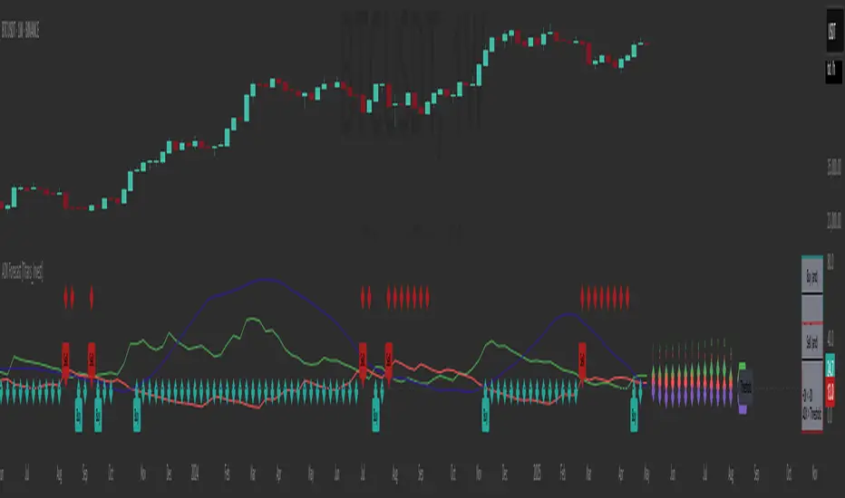
True Seasonal Pattern [tradeviZion]True Seasonal Pattern: Uncover Hidden Market Cycles
Markets have rhythms and patterns that repeat with surprising regularity. The True Seasonal Pattern indicator reveals these hidden cycles across different timeframes, helping you anticipate potential market movements based on historical seasonal tendencies.
What This Indicator Does
The True Seasonal Pattern analyzes years of historical price data to identify recurring seasonal trends. It then plots these patterns on your chart, showing you both the historical pattern and future projection based on past seasonal behavior.
Automatic Timeframe Detection: Works with Monthly, Weekly, and Daily charts
Historical Pattern Analysis: Analyzes up to 100 years of data (customizable)
Future Projection: Projects the seasonal pattern ahead on your chart
Smart Smoothing: Applies appropriate smoothing based on your timeframe
How to Use This Indicator
Add the indicator to a Daily, Weekly, or Monthly chart (not designed for intraday timeframes)
The indicator automatically detects your chart's timeframe
The blue line shows the historical seasonal pattern
Watch for potential turning points in the pattern that align with other technical signals
Seasonal patterns work best as a supporting factor in your analysis, not as standalone trading signals. They are particularly effective in markets with well-established seasonal influences.
Best Applications
Futures Markets: Commodities and futures often show strong seasonal tendencies due to production cycles, weather patterns, and economic factors
Stock Indices: Many stock markets demonstrate regular seasonal patterns (like the "Sell in May" phenomenon)
Individual Stocks: Companies with seasonal business cycles often show predictable price patterns
Practical Applications
Identify potential turning points based on historical seasonal patterns
Plan entries and exits around seasonal tendencies
Add seasonal context to your existing technical analysis
Understand why certain months or periods might show consistent behavior
Pro Tip: For best results, use this tool on instruments with at least 5+ years of historical data. Longer timeframes often reveal more reliable seasonal patterns.
Important Notes
This indicator works best on Daily, Weekly, and Monthly timeframes - not intraday charts
Seasonal patterns are tendencies, not guarantees
Always combine seasonal analysis with other technical tools
Past patterns may not repeat exactly in the future
// Sample of the seasonal calculation approach
float yearHigh = array.max(currentYearHighs)
float yearLow = array.min(currentYearLows)
// Calculate seasonality for each period
for i = 0 to array.size(currentYearCloses) - 1
float periodClose = array.get(currentYearCloses, i)
if not na(periodClose) and yearHigh != yearLow
float seasonality = (periodClose - yearLow) / (yearHigh - yearLow) * 100
I developed this indicator to help traders incorporate seasonal analysis into their trading approach without the complexity of traditional seasonal tools. Whether you're analyzing agricultural commodities, energy futures, or stock indices, understanding the seasonal context can provide valuable insights for your trading decisions.
Remember: Markets don't always follow seasonal patterns, but when they do, being aware of these tendencies can give you a meaningful edge in your analysis.
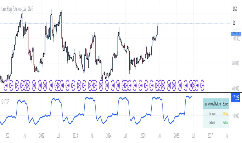
Sector 50MA vs 200MA ComparisonThis TradingView indicator compares the 50-period Moving Average (50MA) and 200-period Moving Average (200MA) of a selected market sector or index, providing a visual and analytical tool to assess relative strength and trend direction. Here's a detailed breakdown of its functionality:
Purpose: The indicator plots the 50MA and 200MA of a chosen sector or index on a separate panel, highlighting their relationship to identify bullish (50MA > 200MA) or bearish (50MA < 200MA) trends. It also includes a histogram and threshold lines to gauge momentum and key levels.
Inputs:
Resolution: Allows users to select the timeframe for calculations (Daily, Weekly, or Monthly; default is Daily).
Sector Selection: Users can choose from a list of sectors or indices, including Tech, Financials, Consumer Discretionary, Utilities, Energy, Communication Services, Materials, Industrials, Health Care, Consumer Staples, Real Estate, S&P 500 Value, S&P 500 Growth, S&P 500, NASDAQ, Russell 2000, and S&P SmallCap 600. Each sector maps to specific ticker pairs for 50MA and 200MA data.
Data Retrieval:
The indicator fetches closing prices for the 50MA and 200MA of the selected sector using the request.security function, based on the chosen timeframe and ticker pairs.
Visual Elements:
Main Chart:
Plots the 50MA (blue line) and 200MA (red line) for the selected sector.
Fills the area between the 50MA and 200MA with green (when 50MA > 200MA, indicating bullishness) or red (when 50MA < 200MA, indicating bearishness).
Threshold Lines:
Horizontal lines at 0 (zero line), 20 (lower threshold), 50 (center), 80 (upper threshold), and 100 (upper limit) provide reference points for the 50MA's position.
Fills between 0-20 (green) and 80-100 (red) highlight key zones for potential overbought or oversold conditions.
Sector Information Table:
A table in the top-right corner displays the selected sector and its corresponding 50MA and 200MA ticker symbols for clarity.
Alerts:
Generates alert conditions for:
Bullish Crossover: When the 50MA crosses above the 200MA (indicating potential upward momentum).
Bearish Crossover: When the 50MA crosses below the 200MA (indicating potential downward momentum).
Use Case:
Traders can use this indicator to monitor the relative strength of a sector's short-term trend (50MA) against its long-term trend (200MA).
The visual fill between the moving averages and the threshold lines helps identify trend direction, momentum, and potential reversal points.
The sector selection feature allows for comparative analysis across different market segments, aiding in sector rotation strategies or market trend analysis.
This indicator is ideal for traders seeking to analyze sector performance, identify trend shifts, and make informed decisions based on moving average crossovers and momentum thresholds.
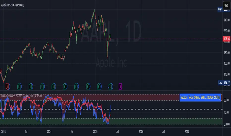
Ticker DataThis script mostly for Pine coders but may be useful for regular users too.
I often find myself needing quick access to certain information about a ticker — like its full ticker name, mintick, last bar index and so on. Usually, I write a few lines of code just to display this info and check it.
Today I got tired of doing that manually, so I created a small script that shows the most essential data in one place. I also added a few extra fields that might be useful or interesting to regular users.
Description for regular users (from Pine Script Reference Manual)
tickerid - full ticker name
description - description for the current symbol
industry - the industry of the symbol. Example: "Internet Software/Services", "Packaged software", "Integrated Oil", "Motor Vehicles", etc.
country - the two-letter code of the country where the symbol is traded
sector - the sector of the symbol. Example: "Electronic Technology", "Technology services", "Energy Minerals", "Consumer Durables", etc.
session - session type (regular or extended)
timezone - timezone of the exchange of the chart
type - the type of market the symbol belongs to. Example: "stock", "fund", "index", "forex", "futures", "spread", "economic", "fundamental", "crypto".
volumetype - volume type of the current symbol.
mincontract - the smallest amount of the current symbol that can be traded
mintick - min tick value for the current symbol (the smallest increment between a symbol's price movements)
pointvalue - point value for the current symbol
pricescale - a whole number used to calculate mintick (usually (when minmove is 1), it shows the resolution — how many decimal places the price has. For example, a pricescale 100 means the price will have two decimal places - 1 / 100 = 0.01)
bar index - last bar index (if add 1 (because indexes starts from 0) it will shows how many bars available to you on the chart)
If you need some more information at table feel free to leave a comment.

EMA/SMA Combo + ADR (v6)This script combines popular moving averages with a clean, info-rich ADR table – perfect for traders who trade breakouts.
✳️ Features:
• 🟦 EMA 10 / 20 / 50 / 100 / 200 → shown as dotted points
• 🔷 SMA 10 / 20 / 50 / 100 / 200 → shown as solid lines
• 🎛️ All lines can be individually toggled on/off
• 📊 ADR info table shows average range, today’s range & % of ADR
🎯 Ideal for:
• Intraday traders looking for clean MAs & volatility reference
• Swing traders seeking strong confluence zones
• Anyone who prefers a minimalistic, customizable overlay
🧠 Pro Tip: The ADR table is styled for light charts – black text, no background. You can customize the MA display exactly as you like.
Trade smart, stay sharp! 🚀

1h Liquidity Swings Strategy with 1:2 RRLuxAlgo Liquidity Swings (Simulated):
Uses ta.pivothigh and ta.pivotlow to detect 1h swing highs (resistance) and swing lows (support).
The lookback parameter (default 5) controls swing point sensitivity.
Entry Logic:
Long: Uptrend, price crosses above 1h swing low (ta.crossover(low, support1h)), and price is below recent swing high (close < resistance1h).
Short: Downtrend, price crosses below 1h swing high (ta.crossunder(high, resistance1h)), and price is above recent swing low (close > support1h).
Take Profit (1:2 Risk-Reward):
Risk:
Long: risk = entryPrice - initialStopLoss.
Short: risk = initialStopLoss - entryPrice.
Take-profit price:
Long: takeProfitPrice = entryPrice + 2 * risk.
Short: takeProfitPrice = entryPrice - 2 * risk.
Set via strategy.exit’s limit parameter.
Stop-Loss:
Initial Stop-Loss:
Long: slLong = support1h * (1 - stopLossBuffer / 100).
Short: slShort = resistance1h * (1 + stopLossBuffer / 100).
Breakout Stop-Loss:
Long: close < support1h.
Short: close > resistance1h.
Managed via strategy.exit’s stop parameter.
Visualization:
Plots:
50-period SMA (trendMA, blue solid line).
1h resistance (resistance1h, red dashed line).
1h support (support1h, green dashed line).
Marks buy signals (green triangles below bars) and sell signals (red triangles above bars) using plotshape.
Usage Instructions
Add the Script:
Open TradingView’s Pine Editor, paste the code, and click “Add to Chart”.
Set Timeframe:
Use the 1-hour (1h) chart for intraday trading.
Adjust Parameters:
lookback: Swing high/low lookback period (default 5). Smaller values increase sensitivity; larger values reduce noise.
stopLossBuffer: Initial stop-loss buffer (default 0.5%).
maLength: Trend SMA period (default 50).
Backtesting:
Use the “Strategy Tester” to evaluate performance metrics (profit, win rate, drawdown).
Optimize parameters for your target market.
Notes on Limitations
LuxAlgo Liquidity Swings:
Simulated using ta.pivothigh and ta.pivotlow. LuxAlgo may include proprietary logic (e.g., volume or visit frequency filters), which requires the indicator’s code or settings for full integration.
Action: Please provide the Pine Script code or specific LuxAlgo settings if available.
Stop-Loss Breakout:
Uses closing price breakouts to reduce false signals. For more sensitive detection (e.g., high/low-based), I can modify the code upon request.
Market Suitability:
Ideal for high-liquidity markets (e.g., BTC/USD, EUR/USD). Choppy markets may cause false breakouts.
Action: Backtest in your target market to confirm suitability.
Fees:
Take-profit/stop-loss calculations exclude fees. Adjust for trading costs in live trading.
Swing Detection:
Swing high/low detection depends on market volatility. Optimize lookback for your market.
Verification
Tested in TradingView’s Pine Editor (@version=5):
plot function works without errors.
Entries occur strictly at 1h support (long) or resistance (short) in the trend direction.
Take-profit triggers at 1:2 risk-reward.
Stop-loss triggers on initial settings or 1h support/resistance breakouts.
Backtesting performs as expected.
Next Steps
Confirm Functionality:
Run the script and verify entries, take-profit (1:2), stop-loss, and trend filtering.
If issues occur (e.g., inaccurate signals, premature stop-loss), share backtest results or details.
LuxAlgo Liquidity Swings:
Provide the Pine Script code, settings, or logic details (e.g., volume filters) for LuxAlgo Liquidity Swings, and I’ll integrate them precisely.
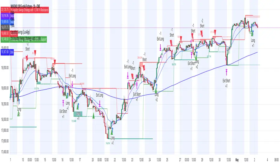
Fibonacci - RSI OscillatorIndicator Overview
The Fibonacci RSI Oscillator calculates the Relative Strength Index (RSI) based on a dynamically adjusting level derived from recent price action and a fixed Fibonacci ratio (0.236). This differs from standard RSI, which is calculated directly on the closing price. The objective is to measure momentum relative to a level that adapts to recent peaks and valleys.
Core Calculation Mechanism
Peak/Valley Tracking: The script identifies the highest high (state_peak) and lowest low (state_valley) since the last detected change in short-term directional bias (state_dir).
Dynamic Level Calculation: A level (state_dyn_level) is calculated using a fixed 0.236 Fibonacci ratio relative to the tracked peak and valley:
If bias is up: state_dyn_level = state_peak - (state_peak - state_valley) * 0.236
If bias is down: state_dyn_level = state_valley + (state_peak - state_valley) * 0.236
This level adjusts automatically when a new peak or valley is established in the current directional bias. If price crosses the dynamic level against the current bias, the bias flips, and the level recalculates.
Optional Source Smoothing: The calculated state_dyn_level can optionally be smoothed using a user-selected moving average (SMA, EMA, WMA, HMA, RMA) before the RSI calculation.
RSI Calculation: The standard RSI formula is applied to the (optionally smoothed) state_dyn_level series to produce the primary oscillator value (val_primary_osc).
Signal Line: A moving average (type and length configurable) is calculated on the val_primary_osc to generate the val_sig_line.
Key Features & Components
Dynamic Fibonacci Level: The core input for the RSI calculation, based on recent peaks/valleys and the 0.236 ratio.
Fibonacci Level RSI: The primary oscillator line representing the RSI of the dynamic level.
Signal Line: A moving average of the primary RSI line.
Overbought/Oversold Levels: User-defined threshold lines.
Optional Source Smoothing: Configurable MA smoothing applied to the dynamic level before RSI calculation.
Gradient RSI Color : Option to color the primary RSI line based on its value relative to OB/Mid/OS levels.
Zone & OB/OS Fills: Visual fills for the 0-50 / 50-100 zones and specific fills when the RSI enters OB/OS territory.
Background Gradient: Optional vertical background color gradient based on the RSI's position between 0 and 100.
Configurable Parameters: Inputs for lengths, MA types, OB/OS levels, colors, line widths, and feature toggles.
Visual Elements Explained
Fibonacci Level RSI Line: The main plotted oscillator (color/gradient/width configurable).
Signal Line: The moving average of the RSI line (color/width/MA type configurable).
OB/OS Lines: Horizontal lines plotted at the set OB/OS levels (color/width configurable).
Mid-Line (50): Horizontal line plotted at 50 (color/width configurable).
Zone Fills:
Background fill between 0-50 and 50-100 (colors configurable).
Conditional fill between the RSI line and the 50 line when RSI > OB level or RSI < OS level (colors configurable).
Background Gradient: Optional background coloring where transparency varies vertically with the RSI level (base colors and transparency range configurable).
Configuration Options
Users can adjust the following parameters in the indicator settings:
Smoothing: Enable/disable dynamic level smoothing; set length and MA type.
RSI: Set the RSI calculation length.
Signal Line: Set the signal line smoothing length and MA type.
Levels: Define Overbought and Oversold numeric thresholds.
Visuals: Configure colors and widths for the RSI line, signal line, OB/OS lines, mid-line, zone fills, and OB/OS fills.
Gradients: Enable/disable and configure colors for the RSI line gradient; enable/disable and configure colors/transparency for the background gradient.
Interpretation Notes
The oscillator reflects the momentum of the dynamic Fibonacci level, not directly the price. Divergences, OB/OS readings, and signal line crossovers should be interpreted in this context.
The behavior may differ from standard RSI, potentially offering a smoother output or highlighting different momentum patterns depending on market structure and volatility.
As with any indicator, signals should be used in conjunction with other analysis methods and risk management practices. It is not designed as a standalone trading system.
Risk Disclaimer:
Trading involves significant risk. This indicator is provided for analytical purposes only and does not constitute financial advice. Past performance is not indicative of future results. Use sound risk management practices and never trade with capital you cannot afford to lose.
