Simplified Market ForecastSimplified Market Forecast Indicator
This indicator pairs nicely with the Contrarian 100 MA and can be located here:
Overview
The "Simplified Market Forecast" (SMF) indicator is a streamlined technical analysis tool designed for traders to identify potential buy and sell opportunities based on a momentum-based oscillator. By analyzing price movements relative to a defined lookback period, SMF generates clear buy and sell signals when the oscillator crosses customizable threshold levels. This indicator is versatile, suitable for various markets (e.g., forex, stocks, cryptocurrencies), and optimized for daily timeframes, though it can be adapted to other timeframes with proper testing. Its intuitive design and visual cues make it accessible for both novice and experienced traders.
How It Works
The SMF indicator calculates a momentum oscillator based on the price’s position within a specified range over a user-defined lookback period. It then smooths this value to reduce noise and plots the result as a line in a separate lower pane. Buy and sell signals are generated when the smoothed oscillator crosses above a user-defined buy level or below a user-defined sell level, respectively. These signals are visualized as triangles either on the main chart or in the lower pane, with a table displaying the current ticker and oscillator value for quick reference.
Key Components
Momentum Oscillator: The indicator measures the price’s position relative to the highest high and lowest low over a specified period, normalized to a 0–100 scale.
Signal Generation: Buy signals occur when the oscillator crosses above the buy level (default: 15), indicating potential oversold conditions. Sell signals occur when the oscillator crosses below the sell level (default: 85), suggesting potential overbought conditions.
Visual Aids: The indicator includes customizable horizontal lines for buy and sell levels, shaded zones for clarity, and a table showing the ticker and current oscillator value.
Mathematical Concepts
Oscillator Calculation: The indicator uses the following formula to compute the raw oscillator value:
c1I = close - lowest(low, medLen)
c2I = highest(high, medLen) - lowest(low, medLen)
fastK_I = (c1I / c2I) * 100
The result is smoothed using a 5-period Simple Moving Average (SMA) to produce the final oscillator value (inter).
Signal Logic:
A buy signal is triggered when the smoothed oscillator crosses above the buy level (ta.crossover(inter, buyLevel)).
A sell signal is triggered when the smoothed oscillator crosses below the sell level (ta.crossunder(inter, sellLevel)).
Entry and Exit Rules
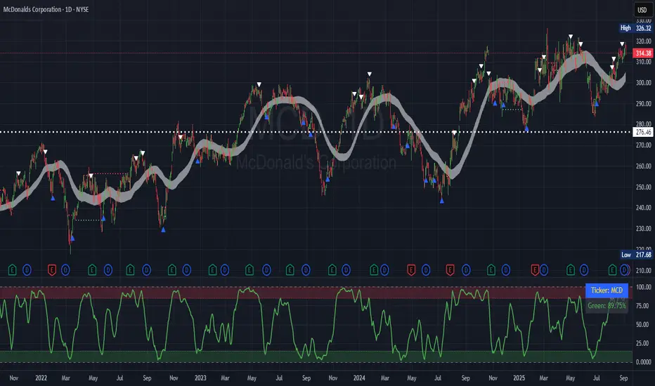
Buy Signal (Blue Triangle): Triggered when the oscillator crosses above the buy level (default: 15), indicating a potential oversold condition and a buying opportunity. The signal appears as a blue triangle either below the price bar (if plotted on the main chart) or at the bottom of the lower pane.
Sell Signal (White Triangle): Triggered when the oscillator crosses below the sell level (default: 85), indicating a potential overbought condition and a selling opportunity. The signal appears as a white triangle either above the price bar (if plotted on the main chart) or at the top of the lower pane.
Exit Rules: Traders can exit positions when an opposite signal occurs (e.g., exit a buy on a sell signal) or based on additional technical analysis tools (e.g., support/resistance, trendlines). Always apply proper risk management.
Recommended Usage
The SMF indicator is optimized for the daily timeframe but can be adapted to other timeframes (e.g., 1H, 4H) with careful testing. It performs best in markets with clear momentum shifts, such as trending or range-bound conditions. Traders should:
Backtest the indicator on their chosen asset and timeframe to validate signal reliability.
Combine with other indicators (e.g., moving averages, support/resistance) or price action for confirmation.
Adjust the lookback period and buy/sell levels to suit market volatility and trading style.
Customization Options
Intermediate Length: Adjust the lookback period for the oscillator calculation (default: 31 bars).
Buy/Sell Levels: Customize the threshold levels for buy (default: 15) and sell (default: 85) signals.
Colors: Modify the colors of the oscillator line, buy/sell signals, and threshold lines.
Signal Display: Toggle whether signals appear on the main chart or in the lower pane.
Visual Aids: The indicator includes dotted horizontal lines at the buy (green) and sell (red) levels, with shaded zones between 0–buy level (green) and sell level–100 (red) for clarity.
Ticker Table: A table in the top-right corner displays the current ticker and oscillator value (in percentage), with customizable colors.
Why Use This Indicator?
The "Simplified Market Forecast" indicator provides a straightforward, momentum-based approach to identifying potential reversals in overbought or oversold markets. Its clear signals, customizable settings, and visual aids make it easy to integrate into various trading strategies. Whether you’re a swing trader or a day trader, SMF offers a reliable tool to enhance decision-making and improve market timing.
Tips for Users
Test the indicator thoroughly on your chosen asset and timeframe to optimize settings.
Use in conjunction with other technical tools for stronger trade confirmation.
Adjust the buy and sell levels based on market conditions (e.g., lower levels for less volatile markets).
Monitor the ticker table for real-time oscillator values to gauge market momentum.
Happy trading with the Simplified Market Forecast indicator!
"摩根纳斯达克100基金风险大吗" için komut dosyalarını ara
Moving Average Adaptive RSI [BackQuant]Moving Average Adaptive RSI
What this is
A momentum oscillator that reshapes classic RSI into a zero-centered column plot and makes it adaptive. It builds RSI from two parts:
• A sensitivity window that scans several recent bars to capture the strongest up and down impulses.
• A selectable moving average that smooths those impulses before computing RSI.
The output ranges roughly from −100 to +100 with 0 as the midline, with optional extra smoothing and built-in divergence detection.
How it works
Impulse extraction
• For each bar the script inspects the last rsi_sen bars and collects upward and downward price changes versus the current price.
• It keeps the maximum upward change and maximum downward change from that window, emphasizing true bursts over single-bar noise.
MA-based averaging
• The up and down impulse series are averaged with your chosen MA over rsi_len bars.
• Supported MA types: SMA, EMA, DEMA, WMA, HMA, SMMA (RMA), TEMA.
Zero-centered RSI transform
• RS = UpMA ÷ DownMA, then mapped to a symmetric scale: 100 − 200 ÷ (1 + RS) .
• Above 0 implies positive momentum bias. Below 0 implies negative momentum bias.
Optional extra smoothing
• A second smoothing pass can be applied to the final oscillator using smoothing_len and smooth_type . Toggle with “Use Extra Smoothing”.
Visual encoding
• The oscillator is drawn as columns around the zero line with a gradient that intensifies toward extremes.
• Static bands mark 80 to 100 and −80 to −100 for extreme conditions.
Key inputs and what they change
• Price Source : input series for momentum.
• Calculation Period (rsi_len) : primary averaging window on up and down components. Higher = smoother, slower.
• Sensitivity (rsi_sen) : how many recent bars are scanned to find max impulses. Higher = more responsive to bursts.
• Calculation Type (ma_type) : MA family that shapes the core behavior. HMA or DEMA is faster, SMA or SMMA is slower.
• Smoothing Type and Length : optional second pass to calm noise on the final output.
• UI toggles : show or hide the oscillator, candle painting, and extreme bands.
Reading the oscillator
• Midline cross up (0) : momentum bias turning positive.
• Midline cross down (0) : momentum bias turning negative.
• Positive territory :
– 0 to 40: constructive but not stretched.
– 40 to 80: strong momentum, continuation more likely.
– Above 80: extreme risk of mean reversion grows.
• Negative territory : mirror the same levels for the downside.
Divergence detection
The script plots four divergence types using pivot highs and lows on both price and the oscillator. Lookbacks are set by lbL and lbR .
• Regular bullish : price lower low, oscillator higher low. Possible downside exhaustion.
• Hidden bullish : price higher low, oscillator lower low. Bias to trend continuation up.
• Regular bearish : price higher high, oscillator lower high. Possible upside exhaustion.
• Hidden bearish : price lower high, oscillator higher high. Bias to trend continuation down.
Labels: ℝ for regular, ℍ for hidden. Green for bullish, red for bearish.
Candle coloring
• Optional bar painting: green when the oscillator is above 0, red when below 0. This is for visual scanning only.
Strengths
• Adaptive sensitivity via a rolling impulse window that responds to genuine bursts.
• Configurable MA core so you can match responsiveness to the instrument.
• Zero-centered scale for simple regime reads with 0 as a clear bias line.
• Built-in regular and hidden divergence mapping.
• Flexible across symbols and timeframes once tuned.
Limitations and cautions
• Trends can remain extended. Treat extremes as context rather than automatic reversal signals.
• Divergence quality depends on pivot lookbacks. Short lookbacks give more signals with more noise. Long lookbacks reduce noise but add lag.
• Double smoothing can delay zero-line transitions. Balance smoothness and timeliness.
Practical usage ideas
• Regime filter : only take long setups from your separate method when the oscillator is above 0, shorts when below 0.
• Pullback confirmation : in uptrends, look for dips that hold above 0 or turn up from 0 to 40. Reverse for downtrends.
• Divergence as a heads-up : wait for a zero-line cross or a price trigger before acting on divergence.
• Sensitivity tuning : start with rsi_sen 2 to 5 on faster timeframes, increase slightly on slower charts.
Alerts
• MA-A RSI Long : oscillator crosses above 0.
• MA-A RSI Short : oscillator crosses below 0.
Use these as bias or timing aids, not standalone trade commands.
Settings quick reference
• Calculation : Price Source, Calculation Type, Calculation Period, Sensitivity.
• Smoothing : Smoothing Type, Smoothing Length, Use Extra Smoothing.
• UI : Show Oscillator, Paint Candles, Show Static High and Low Levels.
• Divergences : Pivot Lookback Left and Right, Div Signal Length, Show Detected Divergences.
Final thoughts
This tool reframes RSI by extracting strong short-term impulses and averaging them with a moving-average model of your choice, then presenting a zero-centered output for clear regime reads. Pair it with your structure, risk and execution process, and tune sensitivity and smoothing to the market you trade.

Infinite EMA with Alpha Control♾️ Infinite EMA with Alpha Control
What Makes This EMA "Infinite"?
Unlike traditional EMA indicators that are limited to typical periods (1-5000), this Infinite EMA breaks all boundaries. You can create EMAs with periods of 1,000, 10,000, or even 1,000,000 bars - that's why it's called "infinite"! Also Infinite EMA starts working immediately from the very first bar on your chart
Why This EMA is "Infinite":
1. Mathematically: When N → ∞, alpha → 0, meaning infinitely long "memory"
2. Practically: You can set any period - even 100,000 bars
3. Flexibility: Alpha allows precise control over the "forgetting speed"
How Does It Work?
The magic lies in the Alpha parameter. While regular EMAs use fixed formulas, this indicator gives you direct control over the EMA's "memory" through Alpha values:
• High Alpha (0.1-0.2): Fast reaction, short memory
• Medium Alpha (0.01-0.05): Balanced response
• Low Alpha (0.0001-0.001): Extremely slow reaction, very long memory
• Ultra-low Alpha (0.000001): Almost frozen in time
The Mathematical Formula:
Alpha = 2 / (Period + 1)
This means you can achieve any EMA period by adjusting Alpha, giving you infinite flexibility!
Expanded "Infinite EMA" Table:
Period EMA (N) - Alpha (Rounded) - Alpha (Exact) - Description
10 - 0.1818 - 0.181818... - Fast EMA
20 - 0.0952 - 0.095238... - Short-term
50 - 0.0392 - 0.039215... - Medium-term
100 - 0.0198 - 0.019801... - Long-term
200 - 0.0100 - 0.009950... - Standard long-term
500 - 0.0040 - 0.003996... - Very long-term
1,000 - 0.0020 - 0.001998... - Super long-term
2,000 - 0.0010 - 0.000999... - Ultra long-term
5,000 - 0.0004 - 0.000399... - Mega long-term
10,000 - 0.0002 - 0.000199... - Giga long-term
25,000 - 0.00008 - 0.000079... - Century-scale EMA
50,000 - 0.00004 - 0.000039... - Practically motionless
100,000 - 0.00002 - 0.000019... - "Glacial" EMA
500,000 - 0.000004 - 0.000003... - Geological timescale
1,000,000 - 0.000002 - 0.000001... - Approaching constant
5,000,000 - 0.0000004 - 0.0000003... - Virtually static
10,000,000 - 0.0000002 - 0.0000001... - Nearly flat line
100,000,000 - 0.00000002 - 0.00000001... - Mathematical infinity
Formula: Alpha = 2/(N+1) where N is the EMA period
Key Features:
Dual EMA System: Run fast and slow EMAs simultaneously
Crossover Signals: Automatic buy/sell signals with customizable alerts
Alpha Control: Direct mathematical control over EMA behavior
Infinite Periods: From 1 to 100,000,000+ bars
Visual Customization: Colors, fills, backgrounds, signal sizes
Instant Start: Works accurately from the very first bar
Update Intervals: Control calculation frequency for noise reduction
Why Choose Infinite EMA?
1. Unlimited Flexibility: Any period you can imagine
2. Mathematical Precision: Direct alpha control for exact behavior
3. Professional Grade: Suitable for all trading styles
4. Easy to Use: Simple settings with powerful results
5. No Warm-up Period: Accurate values from bar #1
Simple Explanation:
Think of EMA as a "memory system":
• High Alpha = Short memory (forgets quickly, reacts fast)
• Low Alpha = Long memory (remembers everything, moves slowly)
With Infinite EMA, you can set the "memory length" to anything from seconds to centuries!
⚡ Instant Start Feature - EMA from First Bar
Immediate Calculation from Bar #1
Unlike traditional EMA indicators that require a "warm-up period" of N bars before showing accurate values, Infinite EMA starts working immediately from the very first bar on your chart.
How It Works:
Traditional EMA Problem:
• Standard 200-period EMA: Needs 200+ bars to become accurate
• First 200 bars: Shows incorrect/unstable values
• Result: Large portions of historical data are unusable
Infinite EMA Solution:
Bar #1: EMA = Current Price (perfect starting point)
Bar #2: EMA = Alpha × Price + (1-Alpha) × Previous EMA
Bar #3: EMA = Alpha × Price + (1-Alpha) × Previous EMA
...and so on
Key Benefits:
No Warm-up Period: Start trading signals from day one
Full Chart Coverage: Every bar has a valid EMA value
Historical Accuracy: Backtesting works on entire dataset
New Markets: Works perfectly on newly listed assets
Short Datasets: Effective even with limited historical data
Practical Impact:
Scenario Traditional EMA Infinite EMA
New cryptocurrency Unusable for first 200 days ✅ Works from day 1
Limited data (< 200 bars) Inaccurate values ✅ Fully functional
Backtesting Must skip first 200 bars ✅ Test entire history
Real-time trading Wait for stabilization ✅ Trade immediately
Technical Implementation:
if barstate.isfirst
EMA := currentPrice // Perfect initialization
else
EMA := alpha × currentPrice + (1-alpha) × previousEMA
This smart initialization ensures mathematical accuracy from the very first calculation, eliminating the traditional EMA "ramp-up" problem.
Why This Matters:
For Backesters: Use 100% of available data
For Live Trading: Get signals immediately on any timeframe
For Researchers: Analyze complete datasets without gaps
Bottom Line: Infinite EMA is ready to work the moment you add it to your chart - no waiting, no warm-up, no exceptions!
Unlike traditional EMAs that require a "warm-up period" of 200+ bars before showing accurate values, Infinite EMA starts working immediately from bar #1.
This breakthrough eliminates the common problem where the first portion of your chart shows unreliable EMA data. Whether you're analyzing a newly listed cryptocurrency, working with limited historical data, or backtesting strategies, every single bar provides mathematically accurate EMA values.
No more waiting periods, no more unusable data sections - just instant, reliable trend analysis from the moment you apply the indicator to any chart.
🔄 Update Interval Bars Feature
The Update Interval feature allows you to control how frequently the EMA recalculates, providing flexible noise filtering without changing the core mathematics.
Set to 1 for standard behavior (updates every bar), or increase to 5-10 for smoother signals that update less frequently. Higher intervals reduce market noise and false signals but introduce slightly more lag. This is particularly useful on volatile timeframes where you want the EMA's directional bias without every minor price fluctuation affecting the calculation.
Perfect for swing traders who prefer cleaner, more stable trend lines over hyper-responsive indicators.
Conclusion
The Infinite EMA transforms the traditional EMA from a fixed-period tool into a precision instrument with unlimited flexibility. By understanding the Alpha-Period relationship, traders can create custom EMAs that perfectly match their trading style, timeframe, and market conditions.
The "infinite" nature comes from the ability to set any period imaginable - from ultra-fast 2-bar EMAs to glacially slow 10-million-bar EMAs, all controlled through a single Alpha parameter.
________________________________________
Whether you're a beginner looking for simple trend following or a professional researcher analyzing century-long patterns, Infinite EMA adapts to your needs. The power of infinite periods is now in your hands! 🚀
Go forward to the horizon. When you reach it, a new one will open up.
- J. P. Morgan

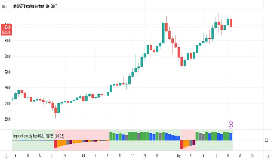
Impulse Convexity Trend Gate [T1][T69]OVERVIEW 🧭
• A price-only trend engine that opens a “gate” only when trend strength, acceleration, and impulse dominance align.
• Built from three cooperating parts: adaptive slope, directional convexity, and an impulse-vs-pullback ratio.
• Output is a bounded oscillator (−100…+100) plus side-specific gate states (bull/bear), with optional pullback and weakness highlights.
THE IDEA & USEFULNESS 🧪
• Not a simple mashup: each component plays a distinct role—slope for direction, convexity for acceleration agreement, and an impulse ratio to suppress correction noise.
• Adaptive EMA length (series-based) lets the midline adjust to conditions without external indicators.
• Approximation of hyperbolic tangent and clamp keep signals bounded and stable while avoiding library dependencies.
• Designed to help trend traders act only when continuation is likely, and stand down during pullbacks or chop.
HOW IT WORKS (PIPELINE) ⚙️
• Price transform
• Uses log price for scale stability.
• Adaptive midline
• Volatility-aware EMA length is clamped between minimum and maximum, then applied via a custom recursive EMA.
• Slope & convexity
• Slope (first difference of the midline) defines direction; convexity (second difference) verifies acceleration agrees with that direction.
• Impulse vs pullback ratio (R)
• Sums directional progress versus counter-direction pullbacks over a window; requires impulse to dominate.
• Normalization & score
• Slope and convexity are normalized by recent dispersion; combined into a raw score and squashed to −100…+100 using manual tanh.
• Trend gate
• Gate opens only when: R ≥ threshold, |normalized slope| ≥ threshold, and slope/convexity share the same sign.
• States & visuals
• Bull/Bear Gate Entry when gate is open, oscillator crosses ±15 in the correct direction, price is on the correct side of the midline, and slope/convexity agree.
• Pullbacks mark counter-moves while a gate is active; Weakness flags specific fade patterns after pullbacks.
FEATURES ✨
• Bull and Bear Gate Entries (green/red columns).
• Pullback shading and optional trend-weakness highlights (yellow/orange + teal/maroon).
• Background tint reflects the active side (bull or bear).
• Pure price logic; no volume or external filters required.
HOW TO USE 🎯
• Regime filter
• Trade only in the direction of the open gate; ignore signals when the gate is closed.
• Pullback entries
• During an open gate, wait for a pullback zone, then act on trend-resumption (e.g., oscillator re-push through ±15 or structure break in gate direction).
• Exits & risk
• Consider trimming when the oscillator relaxes toward 0 while the gate remains open, or when convexity flips against slope and R deteriorates.
• Timeframes & markets
• Suited for trend following on crypto/FX/indices from M30 to 4H/1D; raise thresholds on lower timeframes to reduce noise.
CONFIGURATION 🔧
• Impulse ratio gate (R ≥): raises/lowers the standard for continuation dominance.
• Slope strength gate (|sN| ≥): controls how strong a slope must be to count.
• Show Pullback Impulse (toggle): enable/disable pullback highlights.
• Show Trend Weakness (toggle): enable/disable weakness flags.
LIMITATIONS ⚠️
• As a trend tool, it can lag at regime transitions; expect whipsaws in tight ranges.
• Parameters are instrument- and timeframe-dependent; tune thresholds before live use.
• Pullback/weakness flags are contextual—not trade signals by themselves; use them with gate state and your execution rules.
ADVANCED TIPS 🛠️
• Tighten R and slope thresholds for lower timeframes; loosen for higher timeframes.
• Pair with NNFX-style money management and pair-level filters; let the gate be the confirmation layer, not the entry trigger by itself.
• Batch-test across 100+ symbols, export metrics, and run Monte Carlo to validate LLN reliability and Sharpe/IQR stability.
• For system hedging, disable entries when both sides trigger on the same asset to avoid internal conflict.
NOTES 📝
• Price-only construction reduces data-vendor differences and keeps behavior consistent across markets.
• Manual tanh/clamp ensure stable, bounded scores even during extremes.
DISCLAIMER 🛡️
• For research and education. No financial advice. Test thoroughly, size conservatively, and respect your risk rules.
Stock Profit Calculator — Live Mode
## Overview
This Pine Script indicator calculates, in real time, the financial impact of a stock trade, including purchase/sale commissions, capital gains tax (CGT), and return on investment (ROI). It displays a compact table with key values and also calculates the breakeven price to see at what level the net P/L returns to zero.
---
## Inputs and customization
- **Number of shares:** `shares` defines the purchased quantity.
- **Purchase price:** `buyPrice` is the unit cost; the total purchase is calculated from this.
- **Live selling price:** `sellPrice = close` uses the last bar’s price for live valuation.
- **Fixed or percentage commissions:** `useFixedComm` selects the model.
- **Fixed:** `buyCommFixed`, `sellCommFixed`.
- **Percentage:** `buyCommPct`, `sellCommPct` (applied to notional value).
- **CGT rate:** `cgtRate` is the percentage rate, applied only in case of profit.
- **Table position:** `tablePosition` with predefined options.
- **Visual style:** `colTxt`, `colPos`, `colNeg`, `colBg`, `colHdr`, `colFrame` for text color, positive/negative P/L, background, header, and borders.
> Tip: if your broker uses minimum fees or composite fees, turn on “Use fixed commissions?” and enter the two fixed fees; otherwise, use the percentage model.
---
## Calculation logic
#### Purchase costs
- **Total purchase:**
\
- **Purchase commission:**
\
- **Net entry cost:**
\
#### Sale revenues
- **Total sale (with live price):**
\
- **Sale commission:**
\
- **Net exit revenue:**
\
#### P/L and taxes
- **Gross P/L:**
\
- **CGT (only on positive P/L):**
\
- **Net P/L:**
\
#### ROI
- **Percentage ROI on invested capital:**
\
#### Breakeven
- **Gross breakeven** shown in the table: the unit price that makes the net P/L exactly zero, including purchase cost and an estimate of the sale commission.
\
In the script, if commissions are fixed it adds the fixed sale fee; if percentage-based, the sale component is not included in this row (conservative approximation).
- **Breakeven with tax** (calculated but not shown):
\
Useful when you want the post-CGT result to be exactly zero. Not displayed in the table but ready for use.
> Note: CGT applies only on positive profits; near breakeven, the tax effect is null or only kicks in beyond a threshold. That’s why the script distinguishes between the “gross” and “with tax” versions.
---
## On-screen table
- **Displayed rows:**
- **Purchase:** total net entry cost (with commissions).
- **Sale:** total net exit revenue (with commissions).
- **Gross P/L:** difference between netSell and netBuy.
- **CGT:** estimated tax only if there’s a gain.
- **Net P/L:** P/L after taxes.
- **ROI (%):** percentage return on netBuy.
- **Breakeven:** gross unit breakeven price.
- **Conditional colors:**
- **P/L and ROI:** green for ≥ 0, red for < 0.
- **Headers and cells:** customizable via the color inputs.
- **Efficient refresh:** the table updates only on the last bar via `barstate.islast` to avoid unnecessary redraws.
---
## Behavior and performance
- **Overlay:** displayed on the price chart.
- **Persistent variable:** table is created once with `var table`.
- **Live price:** `sellPrice` follows the current `close`, making P/L, ROI, and breakeven dynamic.
---
## Limitations and suggestions
- **Commission model:** when using percentage commissions, the breakeven in the table doesn’t add the sale percentage fee in the “breakevenPrice” formula. For more precision, you could solve the equation including the percentage fee on exit.
- **Breakeven with tax:** `breakevenWithTax` is a linear estimate; near zero profit, tax may be null. You might choose to display it instead of, or alongside, the gross breakeven.
- **Precision and formatting:** values are shown with `format.mintick`. If the symbol has very small ticks, consider a custom format for better readability.
- **Edge cases:** ROI is undefined if `netBuy = 0` (unlikely in practice but good to note).
> Pro tip: if you want to show the breakeven with tax, add a “Breakeven (post-CGT)” row printing `breakevenWithTax`. If you prefer a single row, replace the shown value with the post-CGT one.
---

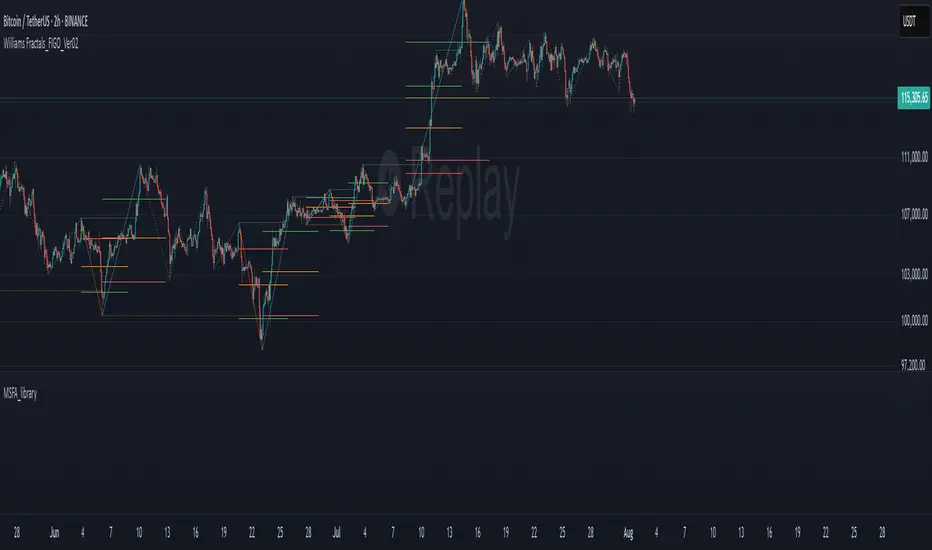
MSFA_LibraryLibrary "MSFA_library"
TODO: add library description here
getDecimals()
Calculates how many decimals are on the quote price of the current market
Returns: The current decimal places on the market quote price
getPipSize(multiplier)
Calculates the pip size of the current market
Parameters:
multiplier (int) : The mintick point multiplier (1 by default, 10 for FX/Crypto/CFD but can be used to override when certain markets require)
Returns: The pip size for the current market
truncate(number, decimalPlaces)
Truncates (cuts) excess decimal places
Parameters:
number (float) : The number to truncate
decimalPlaces (simple float) : (default=2) The number of decimal places to truncate to
Returns: The given number truncated to the given decimalPlaces
toWhole(number)
Converts pips into whole numbers
Parameters:
number (float) : The pip number to convert into a whole number
Returns: The converted number
toPips(number)
Converts whole numbers back into pips
Parameters:
number (float) : The whole number to convert into pips
Returns: The converted number
getPctChange(value1, value2, lookback)
Gets the percentage change between 2 float values over a given lookback period
Parameters:
value1 (float) : The first value to reference
value2 (float) : The second value to reference
lookback (int) : The lookback period to analyze
Returns: The percent change over the two values and lookback period
random(minRange, maxRange)
Wichmann–Hill Pseudo-Random Number Generator
Parameters:
minRange (float) : The smallest possible number (default: 0)
maxRange (float) : The largest possible number (default: 1)
Returns: A random number between minRange and maxRange
bullFib(priceLow, priceHigh, fibRatio)
Calculates a bullish fibonacci value
Parameters:
priceLow (float) : The lowest price point
priceHigh (float) : The highest price point
fibRatio (float) : The fibonacci % ratio to calculate
Returns: The fibonacci value of the given ratio between the two price points
bearFib(priceLow, priceHigh, fibRatio)
Calculates a bearish fibonacci value
Parameters:
priceLow (float) : The lowest price point
priceHigh (float) : The highest price point
fibRatio (float) : The fibonacci % ratio to calculate
Returns: The fibonacci value of the given ratio between the two price points
getMA(length, maType)
Gets a Moving Average based on type (! MUST BE CALLED ON EVERY TICK TO BE ACCURATE, don't place in scopes)
Parameters:
length (simple int) : The MA period
maType (string) : The type of MA
Returns: A moving average with the given parameters
barsAboveMA(lookback, ma)
Counts how many candles are above the MA
Parameters:
lookback (int) : The lookback period to look back over
ma (float) : The moving average to check
Returns: The bar count of how many recent bars are above the MA
barsBelowMA(lookback, ma)
Counts how many candles are below the MA
Parameters:
lookback (int) : The lookback period to look back over
ma (float) : The moving average to reference
Returns: The bar count of how many recent bars are below the EMA
barsCrossedMA(lookback, ma)
Counts how many times the EMA was crossed recently (based on closing prices)
Parameters:
lookback (int) : The lookback period to look back over
ma (float) : The moving average to reference
Returns: The bar count of how many times price recently crossed the EMA (based on closing prices)
getPullbackBarCount(lookback, direction)
Counts how many green & red bars have printed recently (ie. pullback count)
Parameters:
lookback (int) : The lookback period to look back over
direction (int) : The color of the bar to count (1 = Green, -1 = Red)
Returns: The bar count of how many candles have retraced over the given lookback & direction
getBodySize()
Gets the current candle's body size (in POINTS, divide by 10 to get pips)
Returns: The current candle's body size in POINTS
getTopWickSize()
Gets the current candle's top wick size (in POINTS, divide by 10 to get pips)
Returns: The current candle's top wick size in POINTS
getBottomWickSize()
Gets the current candle's bottom wick size (in POINTS, divide by 10 to get pips)
Returns: The current candle's bottom wick size in POINTS
getBodyPercent()
Gets the current candle's body size as a percentage of its entire size including its wicks
Returns: The current candle's body size percentage
isHammer(fib, colorMatch)
Checks if the current bar is a hammer candle based on the given parameters
Parameters:
fib (float) : (default=0.382) The fib to base candle body on
colorMatch (bool) : (default=false) Does the candle need to be green? (true/false)
Returns: A boolean - true if the current bar matches the requirements of a hammer candle
isStar(fib, colorMatch)
Checks if the current bar is a shooting star candle based on the given parameters
Parameters:
fib (float) : (default=0.382) The fib to base candle body on
colorMatch (bool) : (default=false) Does the candle need to be red? (true/false)
Returns: A boolean - true if the current bar matches the requirements of a shooting star candle
isDoji(wickSize, bodySize)
Checks if the current bar is a doji candle based on the given parameters
Parameters:
wickSize (float) : (default=2) The maximum top wick size compared to the bottom (and vice versa)
bodySize (float) : (default=0.05) The maximum body size as a percentage compared to the entire candle size
Returns: A boolean - true if the current bar matches the requirements of a doji candle
isBullishEC(allowance, rejectionWickSize, engulfWick)
Checks if the current bar is a bullish engulfing candle
Parameters:
allowance (float) : (default=0) How many POINTS to allow the open to be off by (useful for markets with micro gaps)
rejectionWickSize (float) : (default=disabled) The maximum rejection wick size compared to the body as a percentage
engulfWick (bool) : (default=false) Does the engulfing candle require the wick to be engulfed as well?
Returns: A boolean - true if the current bar matches the requirements of a bullish engulfing candle
isBearishEC(allowance, rejectionWickSize, engulfWick)
Checks if the current bar is a bearish engulfing candle
Parameters:
allowance (float) : (default=0) How many POINTS to allow the open to be off by (useful for markets with micro gaps)
rejectionWickSize (float) : (default=disabled) The maximum rejection wick size compared to the body as a percentage
engulfWick (bool) : (default=false) Does the engulfing candle require the wick to be engulfed as well?
Returns: A boolean - true if the current bar matches the requirements of a bearish engulfing candle
isInsideBar()
Detects inside bars
Returns: Returns true if the current bar is an inside bar
isOutsideBar()
Detects outside bars
Returns: Returns true if the current bar is an outside bar
barInSession(sess, useFilter)
Determines if the current price bar falls inside the specified session
Parameters:
sess (simple string) : The session to check
useFilter (bool) : (default=true) Whether or not to actually use this filter
Returns: A boolean - true if the current bar falls within the given time session
barOutSession(sess, useFilter)
Determines if the current price bar falls outside the specified session
Parameters:
sess (simple string) : The session to check
useFilter (bool) : (default=true) Whether or not to actually use this filter
Returns: A boolean - true if the current bar falls outside the given time session
dateFilter(startTime, endTime)
Determines if this bar's time falls within date filter range
Parameters:
startTime (int) : The UNIX date timestamp to begin searching from
endTime (int) : the UNIX date timestamp to stop searching from
Returns: A boolean - true if the current bar falls within the given dates
dayFilter(monday, tuesday, wednesday, thursday, friday, saturday, sunday)
Checks if the current bar's day is in the list of given days to analyze
Parameters:
monday (bool) : Should the script analyze this day? (true/false)
tuesday (bool) : Should the script analyze this day? (true/false)
wednesday (bool) : Should the script analyze this day? (true/false)
thursday (bool) : Should the script analyze this day? (true/false)
friday (bool) : Should the script analyze this day? (true/false)
saturday (bool) : Should the script analyze this day? (true/false)
sunday (bool) : Should the script analyze this day? (true/false)
Returns: A boolean - true if the current bar's day is one of the given days
atrFilter(atrValue, maxSize)
Parameters:
atrValue (float)
maxSize (float)
tradeCount()
Calculate total trade count
Returns: Total closed trade count
isLong()
Check if we're currently in a long trade
Returns: True if our position size is positive
isShort()
Check if we're currently in a short trade
Returns: True if our position size is negative
isFlat()
Check if we're currentlyflat
Returns: True if our position size is zero
wonTrade()
Check if this bar falls after a winning trade
Returns: True if we just won a trade
lostTrade()
Check if this bar falls after a losing trade
Returns: True if we just lost a trade
maxDrawdownRealized()
Gets the max drawdown based on closed trades (ie. realized P&L). The strategy tester displays max drawdown as open P&L (unrealized).
Returns: The max drawdown based on closed trades (ie. realized P&L). The strategy tester displays max drawdown as open P&L (unrealized).
totalPipReturn()
Gets the total amount of pips won/lost (as a whole number)
Returns: Total amount of pips won/lost (as a whole number)
longWinCount()
Count how many winning long trades we've had
Returns: Long win count
shortWinCount()
Count how many winning short trades we've had
Returns: Short win count
longLossCount()
Count how many losing long trades we've had
Returns: Long loss count
shortLossCount()
Count how many losing short trades we've had
Returns: Short loss count
breakEvenCount(allowanceTicks)
Count how many break-even trades we've had
Parameters:
allowanceTicks (float) : Optional - how many ticks to allow between entry & exit price (default 0)
Returns: Break-even count
longCount()
Count how many long trades we've taken
Returns: Long trade count
shortCount()
Count how many short trades we've taken
Returns: Short trade count
longWinPercent()
Calculate win rate of long trades
Returns: Long win rate (0-100)
shortWinPercent()
Calculate win rate of short trades
Returns: Short win rate (0-100)
breakEvenPercent(allowanceTicks)
Calculate break even rate of all trades
Parameters:
allowanceTicks (float) : Optional - how many ticks to allow between entry & exit price (default 0)
Returns: Break-even win rate (0-100)
averageRR()
Calculate average risk:reward
Returns: Average winning trade divided by average losing trade
unitsToLots(units)
(Forex) Convert the given unit count to lots (multiples of 100,000)
Parameters:
units (float) : The units to convert into lots
Returns: Units converted to nearest lot size (as float)
skipTradeMonteCarlo(chance, debug)
Checks to see if trade should be skipped to emulate rudimentary Monte Carlo simulation
Parameters:
chance (float) : The chance to skip a trade (0-1 or 0-100, function will normalize to 0-1)
debug (bool) : Whether or not to display a label informing of the trade skip
Returns: True if the trade is skipped, false if it's not skipped (idea being to include this function in entry condition validation checks)
fillCell(tableID, column, row, title, value, bgcolor, txtcolor, tooltip)
This updates the given table's cell with the given values
Parameters:
tableID (table) : The table ID to update
column (int) : The column to update
row (int) : The row to update
title (string) : The title of this cell
value (string) : The value of this cell
bgcolor (color) : The background color of this cell
txtcolor (color) : The text color of this cell
tooltip (string)
Returns: Nothing.
Aetherium Institutional Market Resonance EngineAetherium Institutional Market Resonance Engine (AIMRE)
A Three-Pillar Framework for Decoding Institutional Activity
🎓 THEORETICAL FOUNDATION
The Aetherium Institutional Market Resonance Engine (AIMRE) is a multi-faceted analysis system designed to move beyond conventional indicators and decode the market's underlying structure as dictated by institutional capital flow. Its philosophy is built on a singular premise: significant market moves are preceded by a convergence of context , location , and timing . Aetherium quantifies these three dimensions through a revolutionary three-pillar architecture.
This system is not a simple combination of indicators; it is an integrated engine where each pillar's analysis feeds into a central logic core. A signal is only generated when all three pillars achieve a state of resonance, indicating a high-probability alignment between market organization, key liquidity levels, and cyclical momentum.
⚡ THE THREE-PILLAR ARCHITECTURE
1. 🌌 PILLAR I: THE COHERENCE ENGINE (THE 'CONTEXT')
Purpose: To measure the degree of organization within the market. This pillar answers the question: " Is the market acting with a unified purpose, or is it chaotic and random? "
Conceptual Framework: Institutional campaigns (accumulation or distribution) create a non-random, organized market environment. Retail-driven or directionless markets are characterized by "noise" and chaos. The Coherence Engine acts as a filter to ensure we only engage when institutional players are actively steering the market.
Formulaic Concept:
Coherence = f(Dominance, Synchronization)
Dominance Factor: Calculates the absolute difference between smoothed buying pressure (volume-weighted bullish candles) and smoothed selling pressure (volume-weighted bearish candles), normalized by total pressure. A high value signifies a clear winner between buyers and sellers.
Synchronization Factor: Measures the correlation between the streams of buying and selling pressure over the analysis window. A high positive correlation indicates synchronized, directional activity, while a negative correlation suggests choppy, conflicting action.
The final Coherence score (0-100) represents the percentage of market organization. A high score is a prerequisite for any signal, filtering out unpredictable market conditions.
2. 💎 PILLAR II: HARMONIC LIQUIDITY MATRIX (THE 'LOCATION')
Purpose: To identify and map high-impact institutional footprints. This pillar answers the question: " Where have institutions previously committed significant capital? "
Conceptual Framework: Large institutional orders leave indelible marks on the market in the form of anomalous volume spikes at specific price levels. These are not random occurrences but are areas of intense historical interest. The Harmonic Liquidity Matrix finds these footprints and consolidates them into actionable support and resistance zones called "Harmonic Nodes."
Algorithmic Process:
Footprint Identification: The engine scans the historical lookback period for candles where volume > average_volume * Institutional_Volume_Filter. This identifies statistically significant volume events.
Node Creation: A raw node is created at the mean price of the identified candle.
Dynamic Clustering: The engine uses an ATR-based proximity algorithm. If a new footprint is identified within Node_Clustering_Distance (ATR) of an existing Harmonic Node, it is merged. The node's price is volume-weighted, and its magnitude is increased. This prevents chart clutter and consolidates nearby institutional orders into a single, more significant level.
Node Decay: Nodes that are older than the Institutional_Liquidity_Scanback period are automatically removed from the chart, ensuring the analysis remains relevant to recent market dynamics.
3. 🌊 PILLAR III: CYCLICAL RESONANCE MATRIX (THE 'TIMING')
Purpose: To identify the market's dominant rhythm and its current phase. This pillar answers the question: " Is the market's immediate energy flowing up or down? "
Conceptual Framework: Markets move in waves and cycles of varying lengths. Trading in harmony with the current cyclical phase dramatically increases the probability of success. Aetherium employs a simplified wavelet analysis concept to decompose price action into short, medium, and long-term cycles.
Algorithmic Process:
Cycle Decomposition: The engine calculates three oscillators based on the difference between pairs of Exponential Moving Averages (e.g., EMA8-EMA13 for short cycle, EMA21-EMA34 for medium cycle).
Energy Measurement: The 'energy' of each cycle is determined by its recent volatility (standard deviation). The cycle with the highest energy is designated as the "Dominant Cycle."
Phase Analysis: The engine determines if the dominant cycles are in a bullish phase (rising from a trough) or a bearish phase (falling from a peak).
Cycle Sync: The highest conviction timing signals occur when multiple cycles (e.g., short and medium) are synchronized in the same direction, indicating broad-based momentum.
🔧 COMPREHENSIVE INPUT SYSTEM
Pillar I: Market Coherence Engine
Coherence Analysis Window (10-50, Default: 21): The lookback period for the Coherence Engine.
Lower Values (10-15): Highly responsive to rapid shifts in market control. Ideal for scalping but can be sensitive to noise.
Balanced (20-30): Excellent for day trading, capturing the ebb and flow of institutional sessions.
Higher Values (35-50): Smoother, more stable reading. Best for swing trading and identifying long-term institutional campaigns.
Coherence Activation Level (50-90%, Default: 70%): The minimum market organization required to enable signal generation.
Strict (80-90%): Only allows signals in extremely clear, powerful trends. Fewer, but potentially higher quality signals.
Standard (65-75%): A robust filter that effectively removes choppy conditions while capturing most valid institutional moves.
Lenient (50-60%): Allows signals in less-organized markets. Can be useful in ranging markets but may increase false signals.
Pillar II: Harmonic Liquidity Matrix
Institutional Liquidity Scanback (100-400, Default: 200): How far back the engine looks for institutional footprints.
Short (100-150): Focuses on recent institutional activity, providing highly relevant, immediate levels.
Long (300-400): Identifies major, long-term structural levels. These nodes are often extremely powerful but may be less frequent.
Institutional Volume Filter (1.3-3.0, Default: 1.8): The multiplier for detecting a volume spike.
High (2.5-3.0): Only registers climactic, undeniable institutional volume. Fewer, but more significant nodes.
Low (1.3-1.7): More sensitive, identifying smaller but still relevant institutional interest.
Node Clustering Distance (0.2-0.8 ATR, Default: 0.4): The ATR-based distance for merging nearby nodes.
High (0.6-0.8): Creates wider, more consolidated zones of liquidity.
Low (0.2-0.3): Creates more numerous, precise, and distinct levels.
Pillar III: Cyclical Resonance Matrix
Cycle Resonance Analysis (30-100, Default: 50): The lookback for determining cycle energy and dominance.
Short (30-40): Tunes the engine to faster, shorter-term market rhythms. Best for scalping.
Long (70-100): Aligns the timing component with the larger primary trend. Best for swing trading.
Institutional Signal Architecture
Signal Quality Mode (Professional, Elite, Supreme): Controls the strictness of the three-pillar confluence.
Professional: Loosest setting. May generate signals if two of the three pillars are in strong alignment. Increases signal frequency.
Elite: Balanced setting. Requires a clear, unambiguous resonance of all three pillars. The recommended default.
Supreme: Most stringent. Requires perfect alignment of all three pillars, with each pillar exhibiting exceptionally strong readings (e.g., coherence > 85%). The highest conviction signals.
Signal Spacing Control (5-25, Default: 10): The minimum bars between signals to prevent clutter and redundant alerts.
🎨 ADVANCED VISUAL SYSTEM
The visual architecture of Aetherium is designed not merely for aesthetics, but to provide an intuitive, at-a-glance understanding of the complex data being processed.
Harmonic Liquidity Nodes: The core visual element. Displayed as multi-layered, semi-transparent horizontal boxes.
Magnitude Visualization: The height and opacity of a node's "glow" are proportional to its volume magnitude. More significant nodes appear brighter and larger, instantly drawing the eye to key levels.
Color Coding: Standard nodes are blue/purple, while exceptionally high-magnitude nodes are highlighted in an accent color to denote critical importance.
🌌 Quantum Resonance Field: A dynamic background gradient that visualizes the overall market environment.
Color: Shifts from cool blues/purples (low coherence) to energetic greens/cyans (high coherence and organization), providing instant context.
Intensity: The brightness and opacity of the field are influenced by total market energy (a composite of coherence, momentum, and volume), making powerful market states visually apparent.
💎 Crystalline Lattice Matrix: A geometric web of lines projected from a central moving average.
Mathematical Basis: Levels are projected using multiples of the Golden Ratio (Phi ≈ 1.618) and the ATR. This visualizes the natural harmonic and fractal structure of the market. It is not arbitrary but is based on mathematical principles of market geometry.
🧠 Synaptic Flow Network: A dynamic particle system visualizing the engine's "thought process."
Node Density & Activation: The number of particles and their brightness/color are tied directly to the Market Coherence score. In high-coherence states, the network becomes a dense, bright, and organized web. In chaotic states, it becomes sparse and dim.
⚡ Institutional Energy Waves: Flowing sine waves that visualize market volatility and rhythm.
Amplitude & Speed: The height and speed of the waves are directly influenced by the ATR and volume, providing a feel for market energy.
📊 INSTITUTIONAL CONTROL MATRIX (DASHBOARD)
The dashboard is the central command console, providing a real-time, quantitative summary of each pillar's status.
Header: Displays the script title and version.
Coherence Engine Section:
State: Displays a qualitative assessment of market organization: ◉ PHASE LOCK (High Coherence), ◎ ORGANIZING (Moderate Coherence), or ○ CHAOTIC (Low Coherence). Color-coded for immediate recognition.
Power: Shows the precise Coherence percentage and a directional arrow (↗ or ↘) indicating if organization is increasing or decreasing.
Liquidity Matrix Section:
Nodes: Displays the total number of active Harmonic Liquidity Nodes currently being tracked.
Target: Shows the price level of the nearest significant Harmonic Node to the current price, representing the most immediate institutional level of interest.
Cycle Matrix Section:
Cycle: Identifies the currently dominant market cycle (e.g., "MID ") based on cycle energy.
Sync: Indicates the alignment of the cyclical forces: ▲ BULLISH , ▼ BEARISH , or ◆ DIVERGENT . This is the core timing confirmation.
Signal Status Section:
A unified status bar that provides the final verdict of the engine. It will display "QUANTUM SCAN" during neutral periods, or announce the tier and direction of an active signal (e.g., "◉ TIER 1 BUY ◉" ), highlighted with the appropriate color.
🎯 SIGNAL GENERATION LOGIC
Aetherium's signal logic is built on the principle of strict, non-negotiable confluence.
Condition 1: Context (Coherence Filter): The Market Coherence must be above the Coherence Activation Level. No signals can be generated in a chaotic market.
Condition 2: Location (Liquidity Node Interaction): Price must be actively interacting with a significant Harmonic Liquidity Node.
For a Buy Signal: Price must be rejecting the Node from below (testing it as support).
For a Sell Signal: Price must be rejecting the Node from above (testing it as resistance).
Condition 3: Timing (Cycle Alignment): The Cyclical Resonance Matrix must confirm that the dominant cycles are synchronized with the intended trade direction.
Signal Tiering: The Signal Quality Mode input determines how strictly these three conditions must be met. 'Supreme' mode, for example, might require not only that the conditions are met, but that the Market Coherence is exceptionally high and the interaction with the Node is accompanied by a significant volume spike.
Signal Spacing: A final filter ensures that signals are spaced by a minimum number of bars, preventing over-alerting in a single move.
🚀 ADVANCED TRADING STRATEGIES
The Primary Confluence Strategy: The intended use of the system. Wait for a Tier 1 (Elite/Supreme) or Tier 2 (Professional/Elite) signal to appear on the chart. This represents the alignment of all three pillars. Enter after the signal bar closes, with a stop-loss placed logically on the other side of the Harmonic Node that triggered the signal.
The Coherence Context Strategy: Use the Coherence Engine as a standalone market filter. When Coherence is high (>70%), favor trend-following strategies. When Coherence is low (<50%), avoid new directional trades or favor range-bound strategies. A sharp drop in Coherence during a trend can be an early warning of a trend's exhaustion.
Node-to-Node Trading: In a high-coherence environment, use the Harmonic Liquidity Nodes as both entry points and profit targets. For example, after a BUY signal is generated at one Node, the next Node above it becomes a logical first profit target.
⚖️ RESPONSIBLE USAGE AND LIMITATIONS
Decision Support, Not a Crystal Ball: Aetherium is an advanced decision-support tool. It is designed to identify high-probability conditions based on a model of institutional behavior. It does not predict the future.
Risk Management is Paramount: No indicator can replace a sound risk management plan. Always use appropriate position sizing and stop-losses. The signals provided are probabilistic, not certainties.
Past Performance Disclaimer: The market models used in this script are based on historical data. While robust, there is no guarantee that these patterns will persist in the future. Market conditions can and do change.
Not a "Set and Forget" System: The indicator performs best when its user understands the concepts behind the three pillars. Use the dashboard and visual cues to build a comprehensive view of the market before acting on a signal.
Backtesting is Essential: Before applying this tool to live trading, it is crucial to backtest and forward-test it on your preferred instruments and timeframes to understand its unique behavior and characteristics.
🔮 CONCLUSION
The Aetherium Institutional Market Resonance Engine represents a paradigm shift from single-variable analysis to a holistic, multi-pillar framework. By quantifying the abstract concepts of market context, location, and timing into a unified, logical system, it provides traders with an unprecedented lens into the mechanics of institutional market operations.
It is not merely an indicator, but a complete analytical engine designed to foster a deeper understanding of market dynamics. By focusing on the core principles of institutional order flow, Aetherium empowers traders to filter out market noise, identify key structural levels, and time their entries in harmony with the market's underlying rhythm.
"In all chaos there is a cosmos, in all disorder a secret order." - Carl Jung
— Dskyz, Trade with insight. Trade with confluence. Trade with Aetherium.

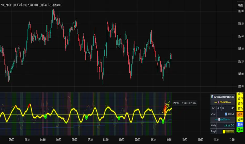
RSI of RSI Deviation (RoRD)RSI of RSI Deviation (RoRD) - Advanced Momentum Acceleration Analysis
What is RSI of RSI Deviation (RoRD)?
RSI of RSI Deviation (RoRD) is a insightful momentum indicator that transcends traditional oscillator analysis by measuring the acceleration of momentum through sophisticated mathematical layering. By calculating RSI on RSI itself (RSI²) and applying advanced statistical deviation analysis with T3 smoothing, RoRD reveals hidden market dynamics that single-layer indicators miss entirely.
This isn't just another RSI variant—it's a complete reimagining of how we measure and visualize momentum dynamics. Where traditional RSI shows momentum, RoRD shows momentum's rate of change . Where others show static overbought/oversold levels, RoRD reveals statistically significant deviations unique to each market's character.
Theoretical Foundation - The Mathematics of Momentum Acceleration
1. RSI² (RSI of RSI) - The Core Innovation
Traditional RSI measures price momentum. RoRD goes deeper:
Primary RSI (RSI₁) : Standard RSI calculation on price
Secondary RSI (RSI²) : RSI calculated on RSI₁ values
This creates a "momentum of momentum" indicator that leads price action
Mathematical Expression:
RSI₁ = 100 - (100 / (1 + RS₁))
RSI² = 100 - (100 / (1 + RS₂))
Where RS₂ = Average Gain of RSI₁ / Average Loss of RSI₁
2. T3 Smoothing - Lag-Free Response
The T3 Moving Average, developed by Tim Tillson, provides:
Superior smoothing with minimal lag
Adaptive response through volume factor (vFactor)
Noise reduction while preserving signal integrity
T3 Formula:
T3 = c1×e6 + c2×e5 + c3×e4 + c4×e3
Where e1...e6 are cascaded EMAs and c1...c4 are volume-factor-based coefficients
3. Statistical Z-Score Deviation
RoRD employs dual-layer Z-score normalization :
Initial Z-Score : (RSI² - SMA) / StDev
Final Z-Score : Z-score of the Z-score for refined extremity detection
This identifies statistically rare events relative to recent market behavior
4. Multi-Timeframe Confluence
Compares current timeframe Z-score with higher timeframe (HTF)
Provides directional confirmation across time horizons
Filters false signals through timeframe alignment
Why RoRD is Different & More Sophisticated
Beyond Traditional Indicators:
Acceleration vs. Velocity : While RSI measures momentum (velocity), RoRD measures momentum's rate of change (acceleration)
Adaptive Thresholds : Z-score analysis adapts to market conditions rather than using fixed 70/30 levels
Statistical Significance : Signals are based on mathematical rarity, not arbitrary levels
Leading Indicator : RSI² often turns before price, providing earlier signals
Reduced Whipsaws : T3 smoothing eliminates noise while maintaining responsiveness
Unique Signal Generation:
Quantum Orbs : Multi-layered visual signals for statistically extreme events
Divergence Detection : Automated identification of price/momentum divergences
Regime Backgrounds : Visual market state classification (Bullish/Bearish/Neutral)
Particle Effects : Dynamic visualization of momentum energy
Visual Design & Interpretation Guide
Color Coding System:
Yellow (#e1ff00) : Neutral/balanced momentum state
Red (#ff0000) : Overbought/extreme bullish acceleration
Green (#2fff00) : Oversold/extreme bearish acceleration
Orange : Z-score visualization
Blue : HTF Z-score comparison
Main Visual Elements:
RSI² Line with Glow Effect
Multi-layer glow creates depth and emphasis
Color dynamically shifts based on momentum state
Line thickness indicates signal strength
Quantum Signal Orbs
Green Orbs Below : Statistically rare oversold conditions
Red Orbs Above : Statistically rare overbought conditions
Multiple layers indicate signal strength
Only appear at Z-score extremes for high-conviction signals
Divergence Markers
Green Circles : Bullish divergence detected
Red Circles : Bearish divergence detected
Plotted at pivot points for precision
Background Regimes
Green Background : Bullish momentum regime
Grey Background : Bearish momentum regime
Blue Background : Neutral/transitioning regime
Particle Effects
Density indicates momentum energy
Color matches current RSI² state
Provides dynamic market "feel"
Dashboard Metrics - Deep Dive
RSI² ANALYSIS Section:
RSI² Value (0-100)
Current smoothed RSI of RSI reading
>70 : Strong bullish acceleration
<30 : Strong bearish acceleration
~50 : Neutral momentum state
RSI¹ Value
Traditional RSI for reference
Compare with RSI² for acceleration/deceleration insights
Z-Score Status
🔥 EXTREME HIGH : Z > threshold, statistically rare bullish
❄️ EXTREME LOW : Z < threshold, statistically rare bearish
📈 HIGH/📉 LOW : Elevated but not extreme
➡️ NEUTRAL : Normal statistical range
MOMENTUM Section:
Velocity Indicator
▲▲▲ : Strong positive acceleration
▼▼▼ : Strong negative acceleration
Shows rate of change in RSI²
Strength Bar
██████░░░░ : Visual power gauge
Filled bars indicate momentum strength
Based on deviation from center line
SIGNALS Section:
Divergence Status
🟢 BULLISH DIV : Price making lows, RSI² making highs
🔴 BEARISH DIV : Price making highs, RSI² making lows
⚪ NO DIVERGENCE : No divergence detected
HTF Comparison
🔥 HTF EXTREME : Higher timeframe confirms extremity
📊 HTF NORMAL : Higher timeframe is neutral
Critical for multi-timeframe confirmation
Trading Application & Strategy
Signal Hierarchy (Highest to Lowest Priority):
Quantum Orb + HTF Alignment + Divergence
Highest conviction reversal signal
Z-score extreme + timeframe confluence + divergence
Quantum Orb + HTF Alignment
Strong reversal signal
Wait for price confirmation
Divergence + Regime Change
Medium-term reversal signal
Monitor for orb confirmation
Threshold Crosses
Traditional overbought/oversold
Use as alert, not entry
Entry Strategies:
For Reversals:
Wait for Quantum Orb signal
Confirm with HTF Z-score direction
Enter on price structure break
Stop beyond recent extreme
For Continuations:
Trade with regime background color
Use RSI² pullbacks to center line
Avoid signals against HTF trend
For Scalping:
Focus on Z-score extremes
Quick entries on orb signals
Exit at center line cross
Risk Management:
Reduce position size when signals conflict with HTF
Avoid trades during regime transitions (blue background)
Tighten stops after divergence completion
Scale out at statistical mean reversion
Development & Uniqueness
RoRD represents months of research into momentum dynamics and statistical analysis. Unlike indicators that simply combine existing tools, RoRD introduces several genuine innovations :
True RSI² Implementation : Not a smoothed RSI, but actual RSI calculated on RSI values
Dual Z-Score Normalization : Unique approach to finding statistical extremes
T3 Integration : First RSI² implementation with T3 smoothing for optimal lag reduction
Quantum Orb Visualization : Revolutionary signal display method
Dynamic Regime Detection : Automatic market state classification
Statistical Adaptability : Thresholds adapt to market volatility
This indicator was built from first principles, with each component carefully selected for its mathematical properties and practical trading utility. The result is a professional-grade tool that provides insights unavailable through traditional momentum analysis.
Best Practices & Tips
Start with default settings - they're optimized for most markets
Always check HTF alignment before taking signals
Use divergences as early warning , orbs as confirmation
Respect regime backgrounds - trade with them, not against
Combine with price action - RoRD shows when, price shows where
Adjust Z-score thresholds based on market volatility
Monitor dashboard metrics for complete market context
Conclusion
RoRD isn't just another indicator—it's a complete momentum analysis system that reveals market dynamics invisible to traditional tools. By combining momentum acceleration, statistical analysis, and multi-timeframe confluence with intuitive visualization, RoRD provides traders with a sophisticated edge in any market condition.
Whether you're scalping rapid reversals or positioning for major trend changes, RoRD's unique approach to momentum analysis will transform how you see and trade market dynamics.
See momentum's future. Trade with statistical edge.
Trade with insight. Trade with anticipation.
— Dskyz, for DAFE Trading Systems
Anomalous Holonomy Field Theory🌌 Anomalous Holonomy Field Theory (AHFT) - Revolutionary Quantum Market Analysis
Where Theoretical Physics Meets Trading Reality
A Groundbreaking Synthesis of Differential Geometry, Quantum Field Theory, and Market Dynamics
🔬 THEORETICAL FOUNDATION - THE MATHEMATICS OF MARKET REALITY
The Anomalous Holonomy Field Theory represents an unprecedented fusion of advanced mathematical physics with practical market analysis. This isn't merely another indicator repackaging old concepts - it's a fundamentally new lens through which to view and understand market structure .
1. HOLONOMY GROUPS (Differential Geometry)
In differential geometry, holonomy measures how vectors change when parallel transported around closed loops in curved space. Applied to markets:
Mathematical Formula:
H = P exp(∮_C A_μ dx^μ)
Where:
P = Path ordering operator
A_μ = Market connection (price-volume gauge field)
C = Closed price path
Market Implementation:
The holonomy calculation measures how price "remembers" its journey through market space. When price returns to a previous level, the holonomy captures what has changed in the market's internal geometry. This reveals:
Hidden curvature in the market manifold
Topological obstructions to arbitrage
Geometric phase accumulated during price cycles
2. ANOMALY DETECTION (Quantum Field Theory)
Drawing from the Adler-Bell-Jackiw anomaly in quantum field theory:
Mathematical Formula:
∂_μ j^μ = (e²/16π²)F_μν F̃^μν
Where:
j^μ = Market current (order flow)
F_μν = Field strength tensor (volatility structure)
F̃^μν = Dual field strength
Market Application:
Anomalies represent symmetry breaking in market structure - moments when normal patterns fail and extraordinary opportunities arise. The system detects:
Spontaneous symmetry breaking (trend reversals)
Vacuum fluctuations (volatility clusters)
Non-perturbative effects (market crashes/melt-ups)
3. GAUGE THEORY (Theoretical Physics)
Markets exhibit gauge invariance - the fundamental physics remains unchanged under certain transformations:
Mathematical Formula:
A'_μ = A_μ + ∂_μΛ
This ensures our signals are gauge-invariant observables , immune to arbitrary market "coordinate changes" like gaps or reference point shifts.
4. TOPOLOGICAL DATA ANALYSIS
Using persistent homology and Morse theory:
Mathematical Formula:
β_k = dim(H_k(X))
Where β_k are the Betti numbers describing topological features that persist across scales.
🎯 REVOLUTIONARY SIGNAL CONFIGURATION
Signal Sensitivity (0.5-12.0, default 2.5)
Controls the responsiveness of holonomy field calculations to market conditions. This parameter directly affects the threshold for detecting quantum phase transitions in price action.
Optimization by Timeframe:
Scalping (1-5min): 1.5-3.0 for rapid signal generation
Day Trading (15min-1H): 2.5-5.0 for balanced sensitivity
Swing Trading (4H-1D): 5.0-8.0 for high-quality signals only
Score Amplifier (10-200, default 50)
Scales the raw holonomy field strength to produce meaningful signal values. Higher values amplify weak signals in low-volatility environments.
Signal Confirmation Toggle
When enabled, enforces additional technical filters (EMA and RSI alignment) to reduce false positives. Essential for conservative strategies.
Minimum Bars Between Signals (1-20, default 5)
Prevents overtrading by enforcing quantum decoherence time between signals. Higher values reduce whipsaws in choppy markets.
👑 ELITE EXECUTION SYSTEM
Execution Modes:
Conservative Mode:
Stricter signal criteria
Higher quality thresholds
Ideal for stable market conditions
Adaptive Mode:
Self-adjusting parameters
Balances signal frequency with quality
Recommended for most traders
Aggressive Mode:
Maximum signal sensitivity
Captures rapid market moves
Best for experienced traders in volatile conditions
Dynamic Position Sizing:
When enabled, the system scales position size based on:
Holonomy field strength
Current volatility regime
Recent performance metrics
Advanced Exit Management:
Implements trailing stops based on ATR and signal strength, with mode-specific multipliers for optimal profit capture.
🧠 ADAPTIVE INTELLIGENCE ENGINE
Self-Learning System:
The strategy analyzes recent trade outcomes and adjusts:
Risk multipliers based on win/loss ratios
Signal weights according to performance
Market regime detection for environmental adaptation
Learning Speed (0.05-0.3):
Controls adaptation rate. Higher values = faster learning but potentially unstable. Lower values = stable but slower adaptation.
Performance Window (20-100 trades):
Number of recent trades analyzed for adaptation. Longer windows provide stability, shorter windows increase responsiveness.
🎨 REVOLUTIONARY VISUAL SYSTEM
1. Holonomy Field Visualization
What it shows: Multi-layer quantum field bands representing market resonance zones
How to interpret:
Blue/Purple bands = Primary holonomy field (strongest resonance)
Band width = Field strength and volatility
Price within bands = Normal quantum state
Price breaking bands = Quantum phase transition
Trading application: Trade reversals at band extremes, breakouts on band violations with strong signals.
2. Quantum Portals
What they show: Entry signals with recursive depth patterns indicating momentum strength
How to interpret:
Upward triangles with portals = Long entry signals
Downward triangles with portals = Short entry signals
Portal depth = Signal strength and expected momentum
Color intensity = Probability of success
Trading application: Enter on portal appearance, with size proportional to portal depth.
3. Field Resonance Bands
What they show: Fibonacci-based harmonic price zones where quantum resonance occurs
How to interpret:
Dotted circles = Minor resonance levels
Solid circles = Major resonance levels
Color coding = Resonance strength
Trading application: Use as dynamic support/resistance, expect reactions at resonance zones.
4. Anomaly Detection Grid
What it shows: Fractal-based support/resistance with anomaly strength calculations
How to interpret:
Triple-layer lines = Major fractal levels with high anomaly probability
Labels show: Period (H8-H55), Price, and Anomaly strength (φ)
⚡ symbol = Extreme anomaly detected
● symbol = Strong anomaly
○ symbol = Normal conditions
Trading application: Expect major moves when price approaches high anomaly levels. Use for precise entry/exit timing.
5. Phase Space Flow
What it shows: Background heatmap revealing market topology and energy
How to interpret:
Dark background = Low market energy, range-bound
Purple glow = Building energy, trend developing
Bright intensity = High energy, strong directional move
Trading application: Trade aggressively in bright phases, reduce activity in dark phases.
📊 PROFESSIONAL DASHBOARD METRICS
Holonomy Field Strength (-100 to +100)
What it measures: The Wilson loop integral around price paths
>70: Strong positive curvature (bullish vortex)
<-70: Strong negative curvature (bearish collapse)
Near 0: Flat connection (range-bound)
Anomaly Level (0-100%)
What it measures: Quantum vacuum expectation deviation
>70%: Major anomaly (phase transition imminent)
30-70%: Moderate anomaly (elevated volatility)
<30%: Normal quantum fluctuations
Quantum State (-1, 0, +1)
What it measures: Market wave function collapse
+1: Bullish eigenstate |↑⟩
0: Superposition (uncertain)
-1: Bearish eigenstate |↓⟩
Signal Quality Ratings
LEGENDARY: All quantum fields aligned, maximum probability
EXCEPTIONAL: Strong holonomy with anomaly confirmation
STRONG: Good field strength, moderate anomaly
MODERATE: Decent signals, some uncertainty
WEAK: Minimal edge, high quantum noise
Performance Metrics
Win Rate: Rolling performance with emoji indicators
Daily P&L: Real-time profit tracking
Adaptive Risk: Current risk multiplier status
Market Regime: Bull/Bear classification
🏆 WHY THIS CHANGES EVERYTHING
Traditional technical analysis operates on 100-year-old principles - moving averages, support/resistance, and pattern recognition. These work because many traders use them, creating self-fulfilling prophecies.
AHFT transcends this limitation by analyzing markets through the lens of fundamental physics:
Markets have geometry - The holonomy calculations reveal this hidden structure
Price has memory - The geometric phase captures path-dependent effects
Anomalies are predictable - Quantum field theory identifies symmetry breaking
Everything is connected - Gauge theory unifies disparate market phenomena
This isn't just a new indicator - it's a new way of thinking about markets . Just as Einstein's relativity revolutionized physics beyond Newton's mechanics, AHFT revolutionizes technical analysis beyond traditional methods.
🔧 OPTIMAL SETTINGS FOR MNQ 10-MINUTE
For the Micro E-mini Nasdaq-100 on 10-minute timeframe:
Signal Sensitivity: 2.5-3.5
Score Amplifier: 50-70
Execution Mode: Adaptive
Min Bars Between: 3-5
Theme: Quantum Nebula or Dark Matter
💭 THE JOURNEY - FROM IMPOSSIBLE THEORY TO TRADING REALITY
Creating AHFT was a mathematical odyssey that pushed the boundaries of what's possible in Pine Script. The journey began with a seemingly impossible question: Could the profound mathematical structures of theoretical physics be translated into practical trading tools?
The Theoretical Challenge:
Months were spent diving deep into differential geometry textbooks, studying the works of Chern, Simons, and Witten. The mathematics of holonomy groups and gauge theory had never been applied to financial markets. Translating abstract mathematical concepts like parallel transport and fiber bundles into discrete price calculations required novel approaches and countless failed attempts.
The Computational Nightmare:
Pine Script wasn't designed for quantum field theory calculations. Implementing the Wilson loop integral, managing complex array structures for anomaly detection, and maintaining computational efficiency while calculating geometric phases pushed the language to its limits. There were moments when the entire project seemed impossible - the script would timeout, produce nonsensical results, or simply refuse to compile.
The Breakthrough Moments:
After countless sleepless nights and thousands of lines of code, breakthrough came through elegant simplifications. The realization that market anomalies follow patterns similar to quantum vacuum fluctuations led to the revolutionary anomaly detection system. The discovery that price paths exhibit holonomic memory unlocked the geometric phase calculations.
The Visual Revolution:
Creating visualizations that could represent 4-dimensional quantum fields on a 2D chart required innovative approaches. The multi-layer holonomy field, recursive quantum portals, and phase space flow representations went through dozens of iterations before achieving the perfect balance of beauty and functionality.
The Balancing Act:
Perhaps the greatest challenge was maintaining mathematical rigor while ensuring practical trading utility. Every formula had to be both theoretically sound and computationally efficient. Every visual had to be both aesthetically pleasing and information-rich.
The result is more than a strategy - it's a synthesis of pure mathematics and market reality that reveals the hidden order within apparent chaos.
📚 INTEGRATED DOCUMENTATION
Once applied to your chart, AHFT includes comprehensive tooltips on every input parameter. The source code contains detailed explanations of the mathematical theory, practical applications, and optimization guidelines. This published description provides the overview - the indicator itself is a complete educational resource.
⚠️ RISK DISCLAIMER
While AHFT employs advanced mathematical models derived from theoretical physics, markets remain inherently unpredictable. No mathematical model, regardless of sophistication, can guarantee future results. This strategy uses realistic commission ($0.62 per contract) and slippage (1 tick) in all calculations. Past performance does not guarantee future results. Always use appropriate risk management and never risk more than you can afford to lose.
🌟 CONCLUSION
The Anomalous Holonomy Field Theory represents a quantum leap in technical analysis - literally. By applying the profound insights of differential geometry, quantum field theory, and gauge theory to market analysis, AHFT reveals structure and opportunities invisible to traditional methods.
From the holonomy calculations that capture market memory to the anomaly detection that identifies phase transitions, from the adaptive intelligence that learns and evolves to the stunning visualizations that make the invisible visible, every component works in mathematical harmony.
This is more than a trading strategy. It's a new lens through which to view market reality.
Trade with the precision of physics. Trade with the power of mathematics. Trade with AHFT.
I hope this serves as a good replacement for Quantum Edge Pro - Adaptive AI until I'm able to fix it.
— Dskyz, Trade with insight. Trade with anticipation.

AWR Pearsons R & LR Oscillator MTF1. Overview
This indicator is designed to analyze the correlation between a price series (or any custom indicator) and the bar index using Pearson’s correlation coefficient. It performs multiple linear regressions over shifted periods and then aggregates these results to create an oscillator. In addition, it integrates a multi-timeframe (MTF) analysis by retrieving the same calculations on 3 different time intervals, providing a more comprehensive view of the trend evolution.
2. User Parameters
The indicator offers several configurable parameters that allow the user to adjust both the calculations and the display:
Source (Linear Regression): The data source on which the regressions are applied (by default, the closing price).
Number of Linear Regressions (numOfLinReg): Allows choosing the number of correlation calculations (up to 10) to be carried out on different shifted periods.
Start Period (startPeriod) and Period Increment (periodIncrement): These parameters define the reference window for each regression. The calculation starts with a base period and then increases with each regression by a fixed increment, creating several time windows to assess the relationship between price evolution and time progression.
Deviation (def_deviation): Although defined, this parameter is intended to control the sensitivity of the calculations. It can be used in further developments of the indicator.
For Multi Time Frames analysis, three additional timeframes are provided through inputs in addition of the current period:
Sum up :
Timeframe 1 = current
Timeframe 2 = 30-minute (default settings)
Timeframe 3 = 1-hour (default settings)
Timeframe 4 = 4-hour (default settings)
These different timeframes allow you to obtain consistent or divergent signals over multiple resolutions, thereby enhancing the confidence of trading decisions.
3. Calculation Logic
At the core of the indicator is the f_calcConditions() function, which performs several essential tasks:
Calculating Pearson's Coefficients For each linear regression, the script uses ta.correlation() to measure the correlation between the chosen source (for example, the closing price) and the chronological index (bar_index). Up to 10 coefficients are computed over shifted windows, providing an evolving view of the linear relationship over different intervals.
Averaging the Results Once the coefficients are calculated, they are stored in an array and averaged to produce a global correlation value called avgPR_local.
Applying Moving Averages
The resulting average is then smoothed using several moving averages (SMA):
A short-term SMA (period of 14),
An intermediate SMA (period of 100),
A long-term SMA (period of 400).
These moving averages help to highlight the underlying trend of the oscillator by indicating the direction in which the correlation is moving.
Defining Trading Conditions Based on avgPR_local and its associated SMAs, multiple conditions are set to generate buy or sell signals:
Simple SMA Conditions :
Small signal :
Light blue below bar signal :
When the averaged coefficients lie between -1 and -0.63, are above the short-term SMA (14 periods), and are increasing, it may indicate a bullish dynamic (buy signal).
Orange above bar signal :
Conversely, when the value is higher (between 0.63 and 1) and below its SMA (14 periods), and are decreasing the trend is considered bearish (sell signal).
Medium signal :
Dark green signal
When the averaged coefficients lie between -1 and -0.45, are above the short-term SMA (14 periods), and are increasing, and also the average 100 is increasing. It may indicate a bullish dynamic (buy signal).
Light red signal :
Conversely, when the value is higher (between 0.45 and 1) and below its SMA (14 periods), the trend and are decreasing, and also the average 100 is decreasing. It may indicate a bearish dynamic(sell signal).
Light green signal :
When the averaged coefficients lie between -1 and -0.15, are above the short-term SMA (14 periods), and are increasing, and also the average 100 & 400 is increasing . It may indicate a bullish dynamic (buy signal).
Dark red signal :
Conversely, when the value is higher (between 0.45 and 1) and below its SMA (14 periods), the trend and are decreasing, and also the average 100 & 400 is decreasing. It may indicate a bearish dynamic(sell signal).
These additional conditions further refine the signals by verifying the consistency of the movement over longer periods. They check that the trends from the respective averages (intermediate and long-term) are in line with the direction indicated by the initial moving average.
These conditions are designed to capture moments when the oscillator's dynamics change, which can be interpreted as opportunities to enter or exit a trade.
4. Multi-Timeframes and Display
One of the main strengths of this indicator is its multi-timeframe approach.
This offers several advantages:
Comparative Analysis: Compare short-term dynamics with broader trends.
Enhanced Signal Reliability: A signal confirmed across multiple timeframes has a higher probability of success.
To visually highlight these signals on the chart, the indicator uses the plotchar() function with distinct symbols for each timeframe:
Current Timeframe: Signals are represented by the character "1"
30-Minute Timeframe: Displayed with the character "2".
1-Hour Timeframe: Displayed with the character "3".
4-Hour Timeframe: Displayed with the character "4".
The colors used are various shades of green for buy signals and shades of red/orange for sell signals, making it easy to distinguish between the different alerts.
5. Integrated Alerts
To avoid missing any trading opportunities, the indicator includes an alert condition via the alertcondition() function. This alert is triggered if any buy or sell signal is generated on any of the analyzed timeframes. The message "MTF valide" indicates that multiple timeframes are confirming the signal, enabling more informed decision-making.
6. How to Use This Indicator
Installation and Configuration: Copy the script into the TradingView Pine Script editor and add it to your chart. The default parameters can be tuned according to market behavior or personal preferences regarding sensitivity and responsiveness.
Interpreting the Signals:
Watch for the symbols on the chart corresponding to each timeframe.
A buy signal appears as a specific symbol below the bar (indicating a bullish condition based on a rising or less negative correlation), while a sell signal appears above the bar.
Multi-Timeframe Analysis: By comparing signals across timeframes, you can filter out false signals. For example, if the short-term timeframe shows a buy signal but the 4-hour timeframe indicates a bearish trend, you may need to reassess your position.
Adjusting the Settings: Depending on the asset type or market volatility, you might need to tweak the periods (startPeriod, periodIncrement) or the number of linear regressions to generate signals that better align with the price dynamics.
Using Alerts: Activate the built-in alert feature so that TradingView notifies you as soon as a multi-timeframe signal is detected. This ensures you stay informed even if you are not continuously monitoring the chart.
In Conclusion
The AWR Pearsons R & LR Oscillator MTF is a powerful tool for traders seeking a detailed understanding of market trends by combining statistical rigor (via Pearson's correlation coefficient) with a multi-timeframe approach. It is capable of generating clear entry and exit signals, visualized with specific symbols and colors depending on the timeframe. By adjusting the parameters to match your trading strategy and leveraging the alert system, you now have a robust instrument for making well-informed market decisions.
Feel free to dive deeper into each component and experiment with different configurations to see how the oscillator integrates with your overall technical analysis strategy. Enjoy exploring its potential and refining your trading approach!

DCA Investment Tracker Pro [tradeviZion]DCA Investment Tracker Pro: Educational DCA Analysis Tool
An educational indicator that helps analyze Dollar-Cost Averaging strategies by comparing actual performance with historical data calculations.
---
💡 Why I Created This Indicator
As someone who practices Dollar-Cost Averaging, I was frustrated with constantly switching between spreadsheets, calculators, and charts just to understand how my investments were really performing. I wanted to see everything in one place - my actual performance, what I should expect based on historical data, and most importantly, visualize where my strategy could take me over the long term .
What really motivated me was watching friends and family underestimate the incredible power of consistent investing. When Napoleon Bonaparte first learned about compound interest, he reportedly exclaimed "I wonder it has not swallowed the world" - and he was right! Yet most people can't visualize how their $500 monthly contributions today could become substantial wealth decades later.
Traditional DCA tracking tools exist, but they share similar limitations:
Require manual data entry and complex spreadsheets
Use fixed assumptions that don't reflect real market behavior
Can't show future projections overlaid on actual price charts
Lose the visual context of what's happening in the market
Make compound growth feel abstract rather than tangible
I wanted to create something different - a tool that automatically analyzes real market history, detects volatility periods, and shows you both current performance AND educational projections based on historical patterns right on your TradingView charts. As Warren Buffett said: "Someone's sitting in the shade today because someone planted a tree a long time ago." This tool helps you visualize your financial tree growing over time.
This isn't just another calculator - it's a visualization tool that makes the magic of compound growth impossible to ignore.
---
🎯 What This Indicator Does
This educational indicator provides DCA analysis tools. Users can input investment scenarios to study:
Theoretical Performance: Educational calculations based on historical return data
Comparative Analysis: Study differences between actual and theoretical scenarios
Historical Projections: Theoretical projections for educational analysis (not predictions)
Performance Metrics: CAGR, ROI, and other analytical metrics for study
Historical Analysis: Calculates historical return data for reference purposes
---
🚀 Key Features
Volatility-Adjusted Historical Return Calculation
Analyzes 3-20 years of actual price data for any symbol
Automatically detects high-volatility stocks (meme stocks, growth stocks)
Uses median returns for volatile stocks, standard CAGR for stable stocks
Provides conservative estimates when extreme outlier years are detected
Smart fallback to manual percentages when data insufficient
Customizable Performance Dashboard
Educational DCA performance analysis with compound growth calculations
Customizable table sizing (Tiny to Huge text options)
9 positioning options (Top/Middle/Bottom + Left/Center/Right)
Theme-adaptive colors (automatically adjusts to dark/light mode)
Multiple display layout options
Future Projection System
Visual future growth projections
Timeframe-aware calculations (Daily/Weekly/Monthly charts)
1-30 year projection options
Shows projected portfolio value and total investment amounts
Investment Insights
Performance vs benchmark comparison
ROI from initial investment tracking
Monthly average return analysis
Investment milestone alerts (25%, 50%, 100% gains)
Contribution tracking and next milestone indicators
---
📊 Step-by-Step Setup Guide
1. Investment Settings 💰
Initial Investment: Enter your starting lump sum (e.g., $60,000)
Monthly Contribution: Set your regular DCA amount (e.g., $500/month)
Return Calculation: Choose "Auto (Stock History)" for real data or "Manual" for fixed %
Historical Period: Select 3-20 years for auto calculations (default: 10 years)
Start Year: When you began investing (e.g., 2020)
Current Portfolio Value: Your actual portfolio worth today (e.g., $150,000)
2. Display Settings 📊
Table Sizes: Choose from Tiny, Small, Normal, Large, or Huge
Table Positions: 9 options - Top/Middle/Bottom + Left/Center/Right
Visibility Toggles: Show/hide Main Table and Stats Table independently
3. Future Projection 🔮
Enable Projections: Toggle on to see future growth visualization
Projection Years: Set 1-30 years ahead for analysis
Live Example - NASDAQ:META Analysis:
Settings shown: $60K initial + $500/month + Auto calculation + 10-year history + 2020 start + $150K current value
---
🔬 Pine Script Code Examples
Core DCA Calculations:
// Calculate total invested over time
months_elapsed = (year - start_year) * 12 + month - 1
total_invested = initial_investment + (monthly_contribution * months_elapsed)
// Compound growth formula for initial investment
theoretical_initial_growth = initial_investment * math.pow(1 + annual_return, years_elapsed)
// Future Value of Annuity for monthly contributions
monthly_rate = annual_return / 12
fv_contributions = monthly_contribution * ((math.pow(1 + monthly_rate, months_elapsed) - 1) / monthly_rate)
// Total expected value
theoretical_total = theoretical_initial_growth + fv_contributions
Volatility Detection Logic:
// Detect extreme years for volatility adjustment
extreme_years = 0
for i = 1 to historical_years
yearly_return = ((price_current / price_i_years_ago) - 1) * 100
if yearly_return > 100 or yearly_return < -50
extreme_years += 1
// Use median approach for high volatility stocks
high_volatility = (extreme_years / historical_years) > 0.2
calculated_return = high_volatility ? median_of_returns : standard_cagr
Performance Metrics:
// Calculate key performance indicators
absolute_gain = actual_value - total_invested
total_return_pct = (absolute_gain / total_invested) * 100
roi_initial = ((actual_value - initial_investment) / initial_investment) * 100
cagr = (math.pow(actual_value / initial_investment, 1 / years_elapsed) - 1) * 100
---
📊 Real-World Examples
See the indicator in action across different investment types:
Stable Index Investments:
AMEX:SPY (SPDR S&P 500) - Shows steady compound growth with standard CAGR calculations
Classic DCA success story: $60K initial + $500/month starting 2020. The indicator shows SPY's historical 10%+ returns, demonstrating how consistent broad market investing builds wealth over time. Notice the smooth theoretical growth line vs actual performance tracking.
MIL:VUAA (Vanguard S&P 500 UCITS) - Shows both data limitation and solution approaches
Data limitation example: VUAA shows "Manual (Auto Failed)" and "No Data" when default 10-year historical setting exceeds available data. The indicator gracefully falls back to manual percentage input while maintaining all DCA calculations and projections.
MIL:VUAA (Vanguard S&P 500 UCITS) - European ETF with successful 5-year auto calculation
Solution demonstration: By adjusting historical period to 5 years (matching available data), VUAA auto calculation works perfectly. Shows how users can optimize settings for newer assets. European market exposure with EUR denomination, demonstrating DCA effectiveness across different markets and currencies.
NYSE:BRK.B (Berkshire Hathaway) - Quality value investment with Warren Buffett's proven track record
Value investing approach: Berkshire Hathaway's legendary performance through DCA lens. The indicator demonstrates how quality companies compound wealth over decades. Lower volatility than tech stocks = standard CAGR calculations used.
High-Volatility Growth Stocks:
NASDAQ:NVDA (NVIDIA Corporation) - Demonstrates volatility-adjusted calculations for extreme price swings
High-volatility example: NVIDIA's explosive AI boom creates extreme years that trigger volatility detection. The indicator automatically switches to "Median (High Vol): 50%" calculations for conservative projections, protecting against unrealistic future estimates based on outlier performance periods.
NASDAQ:TSLA (Tesla) - Shows how 10-year analysis can stabilize volatile tech stocks
Stable long-term growth: Despite Tesla's reputation for volatility, the 10-year historical analysis (34.8% CAGR) shows consistent enough performance that volatility detection doesn't trigger. Demonstrates how longer timeframes can smooth out extreme periods for more reliable projections.
NASDAQ:META (Meta Platforms) - Shows stable tech stock analysis using standard CAGR calculations
Tech stock with stable growth: Despite being a tech stock and experiencing the 2022 crash, META's 10-year history shows consistent enough performance (23.98% CAGR) that volatility detection doesn't trigger. The indicator uses standard CAGR calculations, demonstrating how not all tech stocks require conservative median adjustments.
Notice how the indicator automatically detects high-volatility periods and switches to median-based calculations for more conservative projections, while stable investments use standard CAGR methods.
---
📈 Performance Metrics Explained
Current Portfolio Value: Your actual investment worth today
Expected Value: What you should have based on historical returns (Auto) or your target return (Manual)
Total Invested: Your actual money invested (initial + all monthly contributions)
Total Gains/Loss: Absolute dollar difference between current value and total invested
Total Return %: Percentage gain/loss on your total invested amount
ROI from Initial Investment: How your starting lump sum has performed
CAGR: Compound Annual Growth Rate of your initial investment (Note: This shows initial investment performance, not full DCA strategy)
vs Benchmark: How you're performing compared to the expected returns
---
⚠️ Important Notes & Limitations
Data Requirements: Auto mode requires sufficient historical data (minimum 3 years recommended)
CAGR Limitation: CAGR calculation is based on initial investment growth only, not the complete DCA strategy
Projection Accuracy: Future projections are theoretical and based on historical returns - actual results may vary
Timeframe Support: Works ONLY on Daily (1D), Weekly (1W), and Monthly (1M) charts - no other timeframes supported
Update Frequency: Update "Current Portfolio Value" regularly for accurate tracking
---
📚 Educational Use & Disclaimer
This analysis tool can be applied to various stock and ETF charts for educational study of DCA mathematical concepts and historical performance patterns.
Study Examples: Can be used with symbols like AMEX:SPY , NASDAQ:QQQ , AMEX:VTI , NASDAQ:AAPL , NASDAQ:MSFT , NASDAQ:GOOGL , NASDAQ:AMZN , NASDAQ:TSLA , NASDAQ:NVDA for learning purposes.
EDUCATIONAL DISCLAIMER: This indicator is a study tool for analyzing Dollar-Cost Averaging strategies. It does not provide investment advice, trading signals, or guarantees. All calculations are theoretical examples for educational purposes only. Past performance does not predict future results. Users should conduct their own research and consult qualified financial professionals before making any investment decisions.
---
© 2025 TradeVizion. All rights reserved.
AWR R & LR Oscillator with plots & tableHello trading viewers !
I'm glad to share with you one of my favorite indicator. It's the aggregate of many things. It is partly based on an indicator designed by gentleman goat. Many thanks to him.
1. Oscillator and Correlation Calculations
Overview and Functionality: This part of the indicator computes up to 10 Pearson correlation coefficients between a chosen source (typically the close price, though this is user-configurable) and the bar index over various periods. Starting with an initial period defined by the startPeriod parameter and increasing by a set increment (periodIncrement), each correlation coefficient is calculated using the built-in ta.correlation function over successive ranges. These coefficients are stored in an array, and the indicator calculates their average (avgPR) to provide a complete view of the market trend strength.
Display Features: Each individual coefficient, as well as the overall average, is plotted on the chart using a specific color. Horizontal lines (both dashed and solid) are drawn at levels 0, ±0.8, and ±1, serving as visual thresholds. Additionally, conditional fills in red or blue highlight when values exceed these thresholds, helping the user quickly identify potential extreme conditions (such as overbought or oversold situations).
2. Visual Signals and Automated Alerts
Graphical Signal Enhancements: To reinforce the analysis, the indicator uses graphical elements like emojis and shape markers. For example:
If all 10 curves drop below -0.79, a 🌋 emoji appears at the bottom of the chart;
When curves 2 through 10 are below -0.79, a ⛰️ emoji is displayed below the bar, potentially serving as a buy signal accompanied by an alert condition;
Likewise, symmetrical conditions for correlations exceeding 0.79 produce corresponding emojis (🤿 and 🏖️) at the top or bottom of the chart.
Alerts and Notifications: Using these visual triggers, several alertcondition statements are defined within the script. This allows users to set up TradingView alerts and receive real-time notifications whenever the market reaches these predefined critical zones identified by the multi-period analysis.
3. Regression Channel Analysis
Principles and Calculations: In addition to the oscillator, the indicator implements an analysis of regression channels. For each of the 8 configurable channels, the user can set a range of periods (for example, min1 to max1, etc.). The function calc_regression_channel iterates through the defined period range to find the optimal period that maximizes a statistical measure derived from a regression parameter calculated by the function r(p). Once this optimal period is identified, the indicator computes two key points (A and B) which define the main regression line, and then creates a channel based on the calculated deviation (an RMSE multiplied by a user-defined factor).
The regression channels are not displayed on the chart but are used to plot shapes & fullfilled a table.
Blue shapes are plotted when 6th channel or 7th channel are lower than 3 deviations
Yellow shapes are plotted when 6th channel or 7th channel are higher than 3 deviations
4. Scores, Conditions, and the Summary Table
Scoring System: The indicator goes further by assigning scores across multiple analytical categories, such as:
1. BigPear Score
What It Represents: This score is based on a longer-term moving average of the Pearson correlation values (SMA 100 of the average of the 10 curves of correlation of Pearson). The BigPear category is designed to capture where this longer-term average falls within specific ranges.
Conditions: The script defines nine boolean conditions (labeled BigPear1up through BigPear9up for the “up” direction).
Here's the rules :
BigPear1up = (bigsma_avgPR <= 0.5 and bigsma_avgPR > 0.25)
BigPear2up = (bigsma_avgPR <= 0.25 and bigsma_avgPR > 0)
BigPear3up = (bigsma_avgPR <= 0 and bigsma_avgPR > -0.25)
BigPear4up = (bigsma_avgPR <= -0.25 and bigsma_avgPR > -0.5)
BigPear5up = (bigsma_avgPR <= -0.5 and bigsma_avgPR > -0.65)
BigPear6up = (bigsma_avgPR <= -0.65 and bigsma_avgPR > -0.7)
BigPear7up = (bigsma_avgPR <= -0.7 and bigsma_avgPR > -0.75)
BigPear8up = (bigsma_avgPR <= -0.75 and bigsma_avgPR > -0.8)
BigPear9up = (bigsma_avgPR <= -0.8)
Conditions: The script defines nine boolean conditions (labeled BigPear1down through BigPear9down for the “down” direction).
BigPear1down = (bigsma_avgPR >= -0.5 and bigsma_avgPR < -0.25)
BigPear2down = (bigsma_avgPR >= -0.25 and bigsma_avgPR < 0)
BigPear3down = (bigsma_avgPR >= 0 and bigsma_avgPR < 0.25)
BigPear4down = (bigsma_avgPR >= 0.25 and bigsma_avgPR < 0.5)
BigPear5down = (bigsma_avgPR >= 0.5 and bigsma_avgPR < 0.65)
BigPear6down = (bigsma_avgPR >= 0.65 and bigsma_avgPR < 0.7)
BigPear7down = (bigsma_avgPR >= 0.7 and bigsma_avgPR < 0.75)
BigPear8down = (bigsma_avgPR >= 0.75 and bigsma_avgPR < 0.8)
BigPear9down = (bigsma_avgPR >= 0.8)
Weighting:
If BigPear1up is true, 1 point is added; if BigPear2up is true, 2 points are added; and so on up to 9 points from BigPear9up.
Total Score:
The positive score (posScoreBigPear) is the sum of these weighted conditions.
Similarly, there is a negative score (negScoreBigPear) that is calculated using a mirrored set of conditions (named BigPear1down to BigPear9down), each contributing a negative weight (from -1 to -9).
In essence, the BigPear score tells you—in a weighted cumulative way—where the longer-term correlation average falls relative to predefined thresholds.
2. Pear Score
What It Represents: This category uses the immediate average of the Pearson correlations (avgPR) rather than a longer-term smoothed version. It reflects a more current picture of the market’s correlation behavior.
How It’s Calculated:
Conditions: There are nine conditions defined for the “up” scenario (named Pear1up through Pear9up), which partition the range of avgPR into intervals. For instance:
Pear1up = (avgPR > -0.2 and avgPR <= 0)
Pear2up = (avgPR > -0.4 and avgPR <= -0.2)
Pear3up = (avgPR > -0.5 and avgPR <= -0.4)
Pear4up = (avgPR > -0.6 and avgPR <= -0.5)
Pear5up = (avgPR > -0.65 and avgPR <= -0.6)
Pear6up = (avgPR > -0.7 and avgPR <= -0.65)
Pear7up = (avgPR > -0.75 and avgPR <= -0.7)
Pear8up = (avgPR > -0.8 and avgPR <= -0.75)
Pear9up = (avgPR > -1 and avgPR <= -0.8)
There are nine conditions defined for the “down” scenario (named Pear1down through Pear9down), which partition the range of avgPR into intervals. For instance:
Pear1down = (avgPR >= 0 and avgPR < 0.2)
Pear2down = (avgPR >= 0.2 and avgPR < 0.4)
Pear3down = (avgPR >= 0.4 and avgPR < 0.5)
Pear4down = (avgPR >= 0.5 and avgPR < 0.6)
Pear5down = (avgPR >= 0.6 and avgPR < 0.65)
Pear6down = (avgPR >= 0.65 and avgPR < 0.7)
Pear7down = (avgPR >= 0.7 and avgPR < 0.75)
Pear8down = (avgPR >= 0.75 and avgPR < 0.8)
Pear9down = (avgPR >= 0.8 and avgPR <= 1)
Weighting:
Each condition has an associated weight, such as 0.9 for Pear1up, 1.9 for Pear2up, and so on, up to 9 for Pear9up.
Sum up :
Pear1up = 0.9
Pear2up = 1.9
Pear3up = 2.9
Pear4up = 3.9
Pear5up = 4.99
Pear6up = 6
Pear7up = 7
Pear8up = 8
Pear9up = 9
Total Score:
The positive score (posScorePear) is the sum of these values for each condition that returns true.
A corresponding negative score (negScorePear) is calculated using conditions for when avgPR falls on the positive side, with similar weights in the negative direction.
This score quantifies the current correlation reading by translating its relative level into a numeric score through a weighted sum.
3. Trendpear Score
What It Represents: The Trendpear score is more dynamic as it compares the current avgPR with its short-term moving average (sma_avgPR / 14 periods ) and also considers its relationship with an even longer moving average (bigsma_avgPR / 100 periods). It is meant to capture the trend or momentum in the correlation behavior.
How It’s Calculated:
Conditions: Nine conditions (from Trendpear1up to Trendpear9up) are defined to check:
Whether avgPR is below, equal to, or above sma_avgPR by different margins;
Whether it is trending upward (i.e., it is higher than its previous value).
Here are the rules
Trendpear1up = (avgPR <= sma_avgPR -0.2) and (avgPR >= avgPR )
Trendpear2up = (avgPR > sma_avgPR -0.2) and (avgPR <= sma_avgPR -0.07) and (avgPR >= avgPR )
Trendpear3up = (avgPR > sma_avgPR -0.07) and (avgPR <= sma_avgPR -0.03) and (avgPR >= avgPR )
Trendpear4up = (avgPR > sma_avgPR -0.03) and (avgPR <= sma_avgPR -0.02) and (avgPR >= avgPR )
Trendpear5up = (avgPR > sma_avgPR -0.02) and (avgPR <= sma_avgPR -0.01) and (avgPR >= avgPR )
Trendpear6up = (avgPR > sma_avgPR -0.01) and (avgPR <= sma_avgPR -0.001) and (avgPR >= avgPR )
Trendpear7up = (avgPR >= sma_avgPR) and (avgPR >= avgPR ) and (avgPR <= bigsma_avgPR)
Trendpear8up = (avgPR >= sma_avgPR) and (avgPR >= avgPR ) and (avgPR >= bigsma_avgPR -0.03)
Trendpear9up = (avgPR >= sma_avgPR) and (avgPR >= avgPR ) and (avgPR >= bigsma_avgPR)
Weighting:
The weights here are not linear. For example, the lightest condition may add 0.1 point, whereas the most extreme condition (e.g., when avgPR is not only above the moving average but also reaches a high proportion relative to bigsma_avgPR) might add as much as 90 points.
Trendpear1up = 0.1
Trendpear2up = 0.2
Trendpear3up = 0.3
Trendpear4up = 0.4
Trendpear5up = 0.5
Trendpear6up = 0.69
Trendpear7up = 7
Trendpear8up = 8.9
Trendpear9up = 90
Total Score:
The positive score (posScoreTrendpear) is the sum of the weights from all conditions that are satisfied.
A negative counterpart (negScoreTrendpear) exists similarly for when the trend indicates a downward bias.
Trendpear integrates both the level and the direction of change in the correlations, giving a strong numeric indication when the market starts to diverge from its short-term average.
4. Deviation Score
What It Represents: The “Écart” score quantifies how far the asset’s price deviates from the boundaries defined by the regression channels. This metric can indicate if the price is excessively deviating—which might signal an eventual reversion—or confirming a breakout.
How It’s Calculated:
Conditions: For each channel (with at least seven channels contributing to the scoring from the provided code), there are three levels of deviation:
First tier (EcartXup): Checks if the price is below the upper boundary but above a second boundary.
Second tier (EcartXup2): Checks if the price has dropped further, between a lower and a more extreme boundary.
Third tier (EcartXup3): Checks if the price is below the most extreme limit.
Weighting:
Each tier within a channel has a very small weight for the lowest severities (for example, 0.0001 for the first tier, 0.0002 for the second, 0.0003 for the third) with weights increasing with the channel index.
First channel : 0.0001 to 0.0003 (very short term)
Second channel : 0.001 to 0.003 (short term)
Third channel : 0.01 to 0.03 (short mid term)
4th channel : 0.1 to 0.3 ( mid term)
5th channel: 1 to 3 (long mid term)
6th channel : 10 to 30 (long term)
7th channel : 100 to 300 (very long term)
Total Score:
The overall positive score (posScoreEcart) is the sum of all the weights for conditions met among the first, second, and third tiers.
The corresponding negative score (negScoreEcart) is calculated similarly (using conditions when the price is above the channel boundaries), with the weights being the same in magnitude but negative in sign.
This layered scoring method allows the indicator to reflect both minor and major deviations in a gradated and cumulative manner.
Example :
Score + = 321.0001
Score - = -0.111
The asset price is really overextended in long term view, not for mid term & short term expect the in the very short term.
Score + = 0.0033
Score - = -1.11
The asset price is really extended in short term view, not for mid term (even a bit underextended) & long term is neutral
5. Slope Score
What It Represents: The Slope score captures the trend direction and steepness of the regression channels. It reflects whether the regression line (and hence the underlying trend) is sloping upward or downward.
How It’s Calculated:
Conditions:
if the slope has a uptrend = 1
if the slope has a downtrend = -1
Weighting:
First channel : 0.0001 to 0.0003 (very short term)
Second channel : 0.001 to 0.003 (short term)
Third channel : 0.01 to 0.03 (short mid term)
4th channel : 0.1 to 0.3 ( mid term)
5th channel: 1 to 3 (long mid term)
6th channel : 10 to 30 (long term)
7th channel : 100 to 300 (very long term)
The positive slope conditions incrementally add weights from 0.0001 for the smallest positive slopes to 100 for the largest among the seven checks. And negative for the downward slopes.
The positive score (posScoreSlope) is the sum of all the weights from the upward slope conditions that are met.
The negative score (negScoreSlope) sums the negative weights when downward conditions are met.
Example :
Score + = 111
Score - = -0.1111
Trend is up for longterm & down for mid & short term
The slope score therefore emphasizes both the magnitude and the direction of the trend as indicated by the regression channels, with an intentional asymmetry that flags strong downtrends more aggressively.
Summary
For each category—BigPear, Pear, Trendpear, Écart, and Slope—the indicator evaluates a defined set of conditions. Each condition is a binary test (true/false) based on different thresholds or comparisons (for example, comparing the current value to a moving average or a channel boundary). When a condition is true, its assigned weight is added to the cumulative score for that category. These individual scores, both positive and negative, are then displayed in a table, making it easy for the trader to see at a glance where the market stands according to each analytical dimension.
This comprehensive, weighted approach allows the indicator to encapsulate several layers of market information into a single set of scores, aiding in the identification of potential trading opportunities or market reversals.
5. Practical Use and Application
How to Use the Indicator:
Interpreting the Signals:
On your chart, observe the following components:
The individual correlation curves and their average, plotted with visual thresholds;
Visual markers (such as emojis and shape markers) that signal potential oversold or overbought conditions
The summary table that aggregates the scores from each category, offering a quick glance at the market’s state.
Trading Alerts and Decisions: Set your TradingView alerts through the alertcondition functions provided by the indicator. This way, you receive immediate notifications when critical conditions are met, allowing you to react as soon as the market reaches key levels. This tool is especially beneficial for advanced traders who want to combine multiple technical dimensions to optimize entry and exit points with a confluence of signals.
Conclusion and Additional Insights
In summary, this advanced indicator innovatively combines multi-scale Pearson correlation analysis (via multiple linear regressions) with robust regression channel analysis. It offers a deep and nuanced view of market dynamics by delivering clear visual signals and a comprehensive numerical summary through a built-in score table.
Combine this indicator with other tools (e.g., oscillators, moving averages, volume indicators) to enhance overall strategy robustness.

Mandelbrot-Fibonacci Cascade Vortex (MFCV)Mandelbrot-Fibonacci Cascade Vortex (MFCV) - Where Chaos Theory Meets Sacred Geometry
A Revolutionary Synthesis of Fractal Mathematics and Golden Ratio Dynamics
What began as an exploration into Benoit Mandelbrot's fractal market hypothesis and the mysterious appearance of Fibonacci sequences in nature has culminated in a groundbreaking indicator that reveals the hidden mathematical structure underlying market movements. This indicator represents months of research into chaos theory, fractal geometry, and the golden ratio's manifestation in financial markets.
The Theoretical Foundation
Mandelbrot's Fractal Market Hypothesis Traditional efficient market theory assumes normal distributions and random walks. Mandelbrot proved markets are fractal - self-similar patterns repeating across all timeframes with power-law distributions. The MFCV implements this through:
Hurst Exponent Calculation: H = log(R/S) / log(n/2)
Where:
R = Range of cumulative deviations
S = Standard deviation
n = Period length
This measures market memory:
H > 0.5: Trending (persistent) behavior
H = 0.5: Random walk
H < 0.5: Mean-reverting (anti-persistent) behavior
Fractal Dimension: D = 2 - H
This quantifies market complexity, where higher dimensions indicate more chaotic behavior.
Fibonacci Vortex Theory Markets don't move linearly - they spiral. The MFCV reveals these spirals using Fibonacci sequences:
Vortex Calculation: Vortex(n) = Price + sin(bar_index × φ / Fn) × ATR(Fn) × Volume_Factor
Where:
φ = 0.618 (golden ratio)
Fn = Fibonacci number (8, 13, 21, 34, 55)
Volume_Factor = 1 + (Volume/SMA(Volume,50) - 1) × 0.5
This creates oscillating spirals that contract and expand with market energy.
The Volatility Cascade System
Markets exhibit volatility clustering - Mandelbrot's "Noah Effect." The MFCV captures this through cascading volatility bands:
Cascade Level Calculation: Level(i) = ATR(20) × φ^i
Each level represents a different fractal scale, creating a multi-dimensional view of market structure. The golden ratio spacing ensures harmonic resonance between levels.
Implementation Architecture
Core Components:
Fractal Analysis Engine
Calculates Hurst exponent over user-defined periods
Derives fractal dimension for complexity measurement
Identifies market regime (trending/ranging/chaotic)
Fibonacci Vortex Generator
Creates 5 independent spiral oscillators
Each spiral follows a Fibonacci period
Volume amplification creates dynamic response
Cascade Band System
Up to 8 volatility levels
Golden ratio expansion between levels
Dynamic coloring based on fractal state
Confluence Detection
Identifies convergence of vortex and cascade levels
Highlights high-probability reversal zones
Real-time confluence strength calculation
Signal Generation Logic
The MFCV generates two primary signal types:
Fractal Signals: Generated when:
Hurst > 0.65 (strong trend) AND volatility expanding
Hurst < 0.35 (mean reversion) AND RSI < 35
Trend strength > 0.4 AND vortex alignment
Cascade Signals: Triggered by:
RSI > 60 AND price > SMA(50) AND bearish vortex
RSI < 40 AND price < SMA(50) AND bullish vortex
Volatility expansion AND trend strength > 0.3
Both signals implement a 15-bar cooldown to prevent overtrading.
Advanced Input System
Mandelbrot Parameters:
Cascade Levels (3-8):
Controls number of volatility bands
Crypto: 5-7 (high volatility)
Indices: 4-5 (moderate volatility)
Forex: 3-4 (low volatility)
Hurst Period (20-200):
Lookback for fractal calculation
Scalping: 20-50
Day Trading: 50-100
Swing Trading: 100-150
Position Trading: 150-200
Cascade Ratio (1.0-3.0):
Band width multiplier
1.618: Golden ratio (default)
Higher values for trending markets
Lower values for ranging markets
Fractal Memory (21-233):
Fibonacci retracement lookback
Uses Fibonacci numbers for harmonic alignment
Fibonacci Vortex Settings:
Spiral Periods:
Comma-separated Fibonacci sequence
Fast: "5,8,13,21,34" (scalping)
Standard: "8,13,21,34,55" (balanced)
Extended: "13,21,34,55,89" (swing)
Rotation Speed (0.1-2.0):
Controls spiral oscillation frequency
0.618: Golden ratio (balanced)
Higher = more signals, more noise
Lower = smoother, fewer signals
Volume Amplification:
Enables dynamic spiral expansion
Essential for stocks and crypto
Disable for forex (no central volume)
Visual System Architecture
Cascade Bands:
Multi-level volatility envelopes
Gradient coloring from primary to secondary theme
Transparency increases with distance from price
Fill between bands shows fractal structure
Vortex Spirals:
5 Fibonacci-period oscillators
Blue above price (bullish pressure)
Red below price (bearish pressure)
Multiple display styles: Lines, Circles, Dots, Cross
Dynamic Fibonacci Levels:
Auto-updating retracement levels
Smart update logic prevents disruption near levels
Distance-based transparency (closer = more visible)
Updates every 50 bars or on volatility spikes
Confluence Zones:
Highlighted boxes where indicators converge
Stronger confluence = stronger support/resistance
Key areas for reversal trades
Professional Dashboard System
Main Fractal Dashboard: Displays real-time:
Hurst Exponent with market state
Fractal Dimension with complexity level
Volatility Cascade status
Vortex rotation impact
Market regime classification
Signal strength percentage
Active indicator levels
Vortex Metrics Panel: Shows:
Individual spiral deviations
Convergence/divergence metrics
Real-time vortex positioning
Fibonacci period performance
Fractal Metrics Display: Tracks:
Dimension D value
Market complexity rating
Self-similarity strength
Trend quality assessment
Theory Guide Panel: Educational reference showing:
Mandelbrot principles
Fibonacci vortex concepts
Dynamic trading suggestions
Trading Applications
Trend Following:
High Hurst (>0.65) indicates strong trends
Follow cascade band direction
Use vortex spirals for entry timing
Exit when Hurst drops below 0.5
Mean Reversion:
Low Hurst (<0.35) signals reversal potential
Trade toward vortex spiral convergence
Use Fibonacci levels as targets
Tighten stops in chaotic regimes
Breakout Trading:
Monitor cascade band compression
Watch for vortex spiral alignment
Volatility expansion confirms breakouts
Use confluence zones for targets
Risk Management:
Position size based on fractal dimension
Wider stops in high complexity markets
Tighter stops when Hurst is extreme
Scale out at Fibonacci levels
Market-Specific Optimization
Cryptocurrency:
Cascade Levels: 5-7
Hurst Period: 50-100
Rotation Speed: 0.786-1.2
Enable volume amplification
Stock Indices:
Cascade Levels: 4-5
Hurst Period: 80-120
Rotation Speed: 0.5-0.786
Moderate cascade ratio
Forex:
Cascade Levels: 3-4
Hurst Period: 100-150
Rotation Speed: 0.382-0.618
Disable volume amplification
Commodities:
Cascade Levels: 4-6
Hurst Period: 60-100
Rotation Speed: 0.5-1.0
Seasonal adjustment consideration
Innovation and Originality
The MFCV represents several breakthrough innovations:
First Integration of Mandelbrot Fractals with Fibonacci Vortex Theory
Unique synthesis of chaos theory and sacred geometry
Novel application of Hurst exponent to spiral dynamics
Dynamic Volatility Cascade System
Golden ratio-based band expansion
Multi-timeframe fractal analysis
Self-adjusting to market conditions
Volume-Amplified Vortex Spirals
Revolutionary spiral calculation method
Dynamic response to market participation
Multiple Fibonacci period integration
Intelligent Signal Generation
Cooldown system prevents overtrading
Multi-factor confirmation required
Regime-aware signal filtering
Professional Analytics Dashboard
Institutional-grade metrics display
Real-time fractal analysis
Educational integration
Development Journey
Creating the MFCV involved overcoming numerous challenges:
Mathematical Complexity: Implementing Hurst exponent calculations efficiently
Visual Clarity: Displaying multiple indicators without cluttering
Performance Optimization: Managing array operations and calculations
Signal Quality: Balancing sensitivity with reliability
User Experience: Making complex theory accessible
The result is an indicator that brings PhD-level mathematics to practical trading while maintaining visual elegance and usability.
Best Practices and Guidelines
Start Simple: Use default settings initially
Match Timeframe: Adjust parameters to your trading style
Confirm Signals: Never trade MFCV signals in isolation
Respect Regimes: Adapt strategy to market state
Manage Risk: Use fractal dimension for position sizing
Color Themes
Six professional themes included:
Fractal: Balanced blue/purple palette
Golden: Warm Fibonacci-inspired colors
Plasma: Vibrant modern aesthetics
Cosmic: Dark mode optimized
Matrix: Classic green terminal
Fire: Heat map visualization
Disclaimer
This indicator is for educational and research purposes only. It does not constitute financial advice. While the MFCV reveals deep market structure through advanced mathematics, markets remain inherently unpredictable. Past performance does not guarantee future results.
The integration of Mandelbrot's fractal theory with Fibonacci vortex dynamics provides unique market insights, but should be used as part of a comprehensive trading strategy. Always use proper risk management and never risk more than you can afford to lose.
Acknowledgments
Special thanks to Benoit Mandelbrot for revolutionizing our understanding of markets through fractal geometry, and to the ancient mathematicians who discovered the golden ratio's universal significance.
"The geometry of nature is fractal... Markets are fractal too." - Benoit Mandelbrot
Revealing the Hidden Order in Market Chaos Trade with Mathematical Precision. Trade with MFCV.
— Created with passion for the TradingView community
Trade with insight. Trade with anticipation.
— Dskyz , for DAFE Trading Systems

Enhanced Volume Trend Indicator with BB SqueezeEnhanced Volume Trend Indicator with BB Squeeze: Comprehensive Explanation
The visualization system allows traders to quickly scan multiple securities to identify high-probability setups without detailed analysis of each chart. The progression from squeeze to breakout, supported by volume trend confirmation, offers a systematic approach to identifying trading opportunities.
The script combines multiple technical analysis approaches into a comprehensive dashboard that helps traders make informed decisions by identifying high-probability setups while filtering out noise through its sophisticated confirmation requirements. It combines multiple technical analysis approaches into an integrated visual system that helps traders identify potential trading opportunities while filtering out false signals.
Core Features
1. Volume Analysis Dashboard
The indicator displays various volume-related metrics in customizable tables:
AVOL (After Hours + Pre-Market Volume): Shows extended hours volume as a percentage of the 21-day average volume with color coding for buying/selling pressure. Green indicates buying pressure and red indicates selling pressure.
Volume Metrics: Includes regular volume (VOL), dollar volume ($VOL), relative volume compared to 21-day average (RVOL), and relative volume compared to 90-day average (RVOL90D).
Pre-Market Data: Optional display of pre-market volume (PVOL), pre-market dollar volume (P$VOL), pre-market relative volume (PRVOL), and pre-market price change percentage (PCHG%).
2. Enhanced Volume Trend (VTR) Analysis
The Volume Trend indicator uses adaptive analysis to evaluate buying and selling pressure, combining multiple factors:
MACD (Moving Average Convergence Divergence) components
Volume-to-SMA (Simple Moving Average) ratio
Price direction and market conditions
Volume change rates and momentum
EMA (Exponential Moving Average) alignment and crossovers
Volatility filtering
VTR Visual Indicators
The VTR score ranges from 0-100, with values above 50 indicating bullish conditions and below 50 indicating bearish conditions. This is visually represented by colored circles:
"●" (Filled Circle):
Green: Strong bullish trend (VTR ≥ 80)
Red: Strong bearish trend (VTR ≤ 20)
"◯" (Hollow Circle):
Green: Moderate bullish trend (VTR 65-79)
Red: Moderate bearish trend (VTR 21-35)
"·" (Small Dot):
Green: Weak bullish trend (VTR 55-64)
Red: Weak bearish trend (VTR 36-45)
"○" (Medium Hollow Circle): Neutral conditions (VTR 46-54), shown in gray
In "Both" display mode, the VTR shows both the numerical score (0-100) alongside the appropriate circle symbol.
Enhanced VTR Settings
The Enhanced Volume Trend component offers several advanced customization options:
Adaptive Volume Analysis (volTrendAdaptive):
When enabled, dynamically adjusts volume thresholds based on recent market volatility
Higher volatility periods require proportionally higher volume to generate significant signals
Helps prevent false signals during highly volatile markets
Keep enabled for most trading conditions, especially in volatile markets
Speed of Change Weight (volTrendSpeedWeight, range 0-1):
Controls emphasis on volume acceleration/deceleration rather than absolute levels
Higher values (0.7-1.0): More responsive to new volume trends, better for momentum trading
Lower values (0.2-0.5): Less responsive, better for trend following
Helps identify early volume trends before they fully develop
Momentum Period (volTrendMomentumPeriod, range 2-10):
Defines lookback period for volume change rate calculations
Lower values (2-3): More responsive to recent changes, better for short timeframes
Higher values (7-10): Smoother, better for daily/weekly charts
Directly affects how quickly the indicator responds to new volume patterns
Volatility Filter (volTrendVolatilityFilter):
Adjusts significance of volume by factoring in current price volatility
High volume during high volatility receives less weight
High volume during low volatility receives more weight
Helps distinguish between genuine volume-driven moves and volatility-driven moves
EMA Alignment Weight (volTrendEmaWeight, range 0-1):
Controls importance of EMA alignments in final VTR calculation
Analyzes multiple EMA relationships (5, 10, 21 period)
Higher values (0.7-1.0): Greater emphasis on trend structure
Lower values (0.2-0.5): More focus on pure volume patterns
Display Mode (volTrendDisplayMode):
"Value": Shows only numerical score (0-100)
"Strength": Shows only symbolic representation
"Both": Shows numerical score and symbol together
3. Bollinger Band Squeeze Detection (SQZ)
The BB Squeeze indicator identifies periods of low volatility when Bollinger Bands contract inside Keltner Channels, often preceding significant price movements.
SQZ Visual Indicators
"●" (Filled Circle): Strong squeeze - high probability setup for an impending breakout
Green: Strong squeeze with bullish bias (likely upward breakout)
Red: Strong squeeze with bearish bias (likely downward breakout)
Orange: Strong squeeze with unclear direction
"◯" (Hollow Circle): Moderate squeeze - medium probability setup
Green: With bullish EMA alignment
Red: With bearish EMA alignment
Orange: Without clear directional bias
"-" (Dash): Gray dash indicates no squeeze condition (normal volatility)
The script identifies squeeze conditions through multiple methods:
Bollinger Bands contracting inside Keltner Channels
BB width falling to bottom 20% of recent range (BB width percentile)
Very narrow Keltner Channel (less than 5% of basis price)
Tracking squeeze duration in consecutive bars
Different squeeze strengths are detected:
Strong Squeeze: BB inside KC with tight BB width and narrow KC
Moderate Squeeze: BB inside KC with either tight BB width or narrow KC
No Squeeze: Normal market conditions
4. Breakout Detection System
The script includes two breakout indicators working in sequence:
4.1 Pre-Breakout (PBK) Indicator
Detects potential upcoming breakouts by analyzing multiple factors:
Squeeze conditions lasting 2-3 bars or more
Significant price ranges
Strong volume confirmation
EMA/MACD crossovers
Consistent price direction
PBK Visual Indicators
"●" (Filled Circle): Detected pre-breakout condition
Green: Likely upward breakout (bullish)
Red: Likely downward breakout (bearish)
Orange: Direction not yet clear, but breakout likely
"-" (Dash): Gray dash indicates no pre-breakout condition
The PBK uses sophisticated conditions to reduce false signals including minimum squeeze length, significant price movement, and technical confirmations.
4.2 Breakout (BK) Indicator
Confirms actual breakouts in progress by identifying:
End of squeeze or strong expansion of Bollinger Bands
Volume expansion
Price moving outside Bollinger Bands
EMA crossovers with volume confirmation
MACD crossovers with significant price range
BK Visual Indicators
"●" (Filled Circle): Confirmed breakout in progress
Green: Upward breakout (bullish)
Red: Downward breakout (bearish)
Orange: Unusual breakout pattern without clear direction
"◆" (Diamond): Special breakout conditions (meets some but not all criteria)
"-" (Dash): Gray dash indicates no breakout detected
The BK indicator uses advanced filters for confirmation:
Requires consecutive breakout signals to reduce false positives
Strong volume confirmation requirements (40% above average)
Significant price movement thresholds
Consistency checks between price action and indicators
5. Market Metrics and Analysis
Price Change Percentage (CHG%)
Displays the current percentage change relative to the previous day's close, color-coded green for positive changes and red for negative changes.
Average Daily Range (ADR%)
Calculates the average daily percentage range over a specified period (default 20 days), helping traders gauge volatility and set appropriate price targets.
Average True Range (ATR)
Shows the Average True Range value, a volatility indicator developed by J. Welles Wilder that measures market volatility by decomposing the entire range of an asset price for that period.
Relative Strength Index (RSI)
Displays the standard 14-period RSI, a momentum oscillator that measures the speed and change of price movements on a scale from 0 to 100.
6. External Market Indicators
QQQ Change
Shows the percentage change in the Invesco QQQ Trust (tracking the Nasdaq-100 Index), useful for understanding broader tech market trends.
UVIX Change
Displays the percentage change in UVIX, a volatility index, providing insight into market fear and potential hedging activity.
BTC-USD
Shows the current Bitcoin price from Coinbase, useful for traders monitoring crypto correlation with equities.
Market Breadth (BRD)
Calculates the percentage difference between ATHI.US and ATLO.US (high vs. low securities), indicating overall market direction and strength.
7. Session Analysis and Volume Direction
Session Detection
The script accurately identifies different market sessions:
Pre-market: 4:00 AM to 9:30 AM
Regular market: 9:30 AM to 4:00 PM
After-hours: 4:00 PM to 8:00 PM
Closed: Outside trading hours
This detection works on any timeframe through careful calculation of current time in seconds.
Buy/Sell Volume Direction
The script analyzes buying and selling pressure by:
Counting up volume when close > open
Counting down volume when close < open
Tracking accumulated volume within the day
Calculating intraday pressure (up volume minus down volume)
Enhanced AVOL Calculation
The improved AVOL calculation works in all timeframes by:
Estimating typical pre-market and after-hours volume percentages
Combining yesterday's after-hours with today's pre-market volume
Calculating this as a percentage of the 21-day average volume
Determining buying/selling pressure by analyzing after-hours and pre-market price changes
Color-coding results: green for buying pressure, red for selling pressure
This calculation is particularly valuable because it works consistently across any timeframe.
Customization Options
Display Settings
The dashboard has two customizable tables: Volume Table and Metrics Table, with positions selectable as bottom_left or bottom_right.
All metrics can be individually toggled on/off:
Pre-market data (PVOL, P$VOL, PRVOL, PCHG%)
Volume data (AVOL, RVOL Day, RVOL 90D, Volume, SEED_YASHALGO_NSE_BREADTH:VOLUME )
Price metrics (ADR%, ATR, RSI, Price Change%)
Market indicators (QQQ, UVIX, Breadth, BTC-USD)
Analysis indicators (Volume Trend, BB Squeeze, Pre-Breakout, Breakout)
These toggle options allow traders to customize the dashboard to show only the metrics they find most valuable for their trading style.
Table and Text Customization
The dashboard's appearance can be customized:
Table background color via tableBgColor
Text color (White or Black) via textColorOption
The indicator uses smart formatting for volume and price values, automatically adding appropriate suffixes (K, M, B) for readability.
MACD Configuration for VTR
The Volume Trend calculation incorporates MACD with customizable parameters:
Fast Length: Controls the period for the fast EMA (default 3)
Slow Length: Controls the period for the slow EMA (default 9)
Signal Length: Controls the period for the signal line EMA (default 5)
MACD Weight: Controls how much influence MACD has on the volume trend score (default 0.3)
These settings allow traders to fine-tune how momentum is factored into the volume trend analysis.
Bollinger Bands and Keltner Channel Settings
The Bollinger Bands and Keltner Channels used for squeeze detection have preset (hidden) parameters:
BB Length: 20 periods
BB Multiplier: 2.0 standard deviations
Keltner Length: 20 periods
Keltner Multiplier: 1.5 ATR
These settings follow standard practice for squeeze detection while maintaining simplicity in the user interface.
Practical Trading Applications
Complete Trading Strategies
1. Squeeze Breakout Strategy
This strategy combines multiple components of the indicator:
Wait for a strong squeeze (SQZ showing ●)
Look for pre-breakout confirmation (PBK showing ● in green or red)
Enter when breakout is confirmed (BK showing ● in same direction)
Use VTR to confirm volume supports the move (VTR ≥ 65 for bullish or ≤ 35 for bearish)
Set profit targets based on ADR (Average Daily Range)
Exit when VTR begins to weaken or changes direction
2. Volume Divergence Strategy
This strategy focuses on the volume trend relative to price:
Identify when price makes a new high but VTR fails to confirm (divergence)
Look for VTR to show weakening trend (● changing to ◯ or ·)
Prepare for potential reversal when SQZ begins to form
Enter counter-trend position when PBK confirms reversal direction
Use external indicators (QQQ, BTC, Breadth) to confirm broader market support
3. Pre-Market Edge Strategy
This strategy leverages pre-market data:
Monitor AVOL for unusual pre-market activity (significantly above 100%)
Check pre-market price change direction (PCHG%)
Enter position at market open if VTR confirms direction
Use SQZ to determine if volatility is likely to expand
Exit based on RVOL declining or price reaching +/- ADR for the day
Market Context Integration
The indicator provides valuable context for trading decisions:
QQQ change shows tech market direction
BTC price shows crypto market correlation
UVIX change indicates volatility expectations
Breadth measurement shows market internals
This context helps traders avoid fighting the broader market and align trades with overall market direction.
Timeframe Optimization
The indicator is designed to work across different timeframes:
For day trading: Focus on AVOL, VTR, PBK/BK, and use shorter momentum periods
For swing trading: Focus on SQZ duration, VTR strength, and broader market indicators
For position trading: Focus on larger VTR trends and use EMA alignment weight
Advanced Analytical Components
Enhanced Volume Trend Score Calculation
The VTR score calculation is sophisticated, with the base score starting at 50 and adjusting for:
Price direction (up/down)
Volume relative to average (high/normal/low)
Volume acceleration/deceleration
Market conditions (bull/bear)
Additional factors are then applied, including:
MACD influence weighted by strength and direction
Volume change rate influence (speed)
Price/volume divergence effects
EMA alignment scores
Volatility adjustments
Breakout strength factors
Price action confirmations
The final score is clamped between 0-100, with values above 50 indicating bullish conditions and below 50 indicating bearish conditions.
Anti-False Signal Filters
The indicator employs multiple techniques to reduce false signals:
Requiring significant price range (minimum percentage movement)
Demanding strong volume confirmation (significantly above average)
Checking for consistent direction across multiple indicators
Requiring prior bar consistency (consecutive bars moving in same direction)
Counting consecutive signals to filter out noise
These filters help eliminate noise and focus on high-probability setups.
MACD Enhancement and Integration
The indicator enhances standard MACD analysis:
Calculating MACD relative strength compared to recent history
Normalizing MACD slope relative to volatility
Detecting MACD acceleration for stronger signals
Integrating MACD crossovers with other confirmation factors
EMA Analysis System
The indicator uses a comprehensive EMA analysis system:
Calculating multiple EMAs (5, 10, 21 periods)
Detecting golden cross (10 EMA crosses above 21 EMA)
Detecting death cross (10 EMA crosses below 21 EMA)
Assessing price position relative to EMAs
Measuring EMA separation percentage
Recent Enhancements and Evolution
Version 5.2 includes several improvements:
Enhanced AVOL to show buying/selling direction through color coding
Improved VTR with adaptive analysis based on market conditions
AVOL display now works in all timeframes through sophisticated estimation
Removed animal symbols and streamlined code with bright colors for better visibility
Improved anti-false signal filters throughout the system
Optimizing Indicator Settings
For Different Market Types
Range-Bound Markets:
Lower EMA Alignment Weight (0.2-0.4)
Higher Speed of Change Weight (0.8-1.0)
Focus on SQZ and PBK signals for breakout potential
Trending Markets:
Higher EMA Alignment Weight (0.7-1.0)
Moderate Speed of Change Weight (0.4-0.6)
Focus on VTR strength and BK confirmations
Volatile Markets:
Enable Volatility Filter
Enable Adaptive Volume Analysis
Lower Momentum Period (2-3)
Focus on strong volume confirmation (VTR ≥ 80 or ≤ 20)
For Different Asset Classes
Equities:
Standard settings work well
Pay attention to AVOL for gap potential
Monitor QQQ correlation
Futures:
Consider higher Volume/RVOL weight
Reduce MACD weight slightly
Pay close attention to SQZ duration
Crypto:
Higher volatility thresholds may be needed
Monitor BTC price for correlation
Focus on stronger confirmation signals
Integrated Visual System for Trading Decisions
The colored circle indicators create an intuitive visual system for quick market assessment:
Progression Sequence: SQZ (Squeeze) → PBK (Pre-Breakout) → BK (Breakout)
This sequence often occurs in order, with the squeeze leading to pre-breakout conditions, followed by an actual breakout.
VTR (Volume Trend): Provides context about the volume supporting these movements.
Color Coding: Green for bullish conditions, red for bearish conditions, and orange/gray for neutral or undefined conditions.
True Strength Index (TSI)%📌 Script Name: TSI Percentuale
This script is a custom True Strength Index (TSI) indicator that expresses momentum strength as a percentage from 0% to 100%, instead of the traditional TSI scale.
✅ What the Script Does
Calculates the standard TSI:
Uses double exponential smoothing of price changes and their absolute values.
Formula:
TSI_raw
=
100
×
DoubleSmoothed(ΔPrice)
DoubleSmoothed(|ΔPrice|)
TSI_raw=100×
DoubleSmoothed(|ΔPrice|)
DoubleSmoothed(ΔPrice)
Normalizes TSI to a percentile scale:
Over a user-defined lookback period, the script finds the lowest and highest TSI values.
It then rescales the current TSI to a value between 0% (minimum) and 100% (maximum).
50% represents neutral momentum (i.e., "flat").
Plots the result:
tsi_percent is plotted as a blue line.
Horizontal dashed/dotted lines are drawn at:
0% → strong downward momentum
50% → neutral
100% → strong upward momentum
⚙️ Inputs
Long Length: Long EMA smoothing period (default: 25)
Short Length: Short EMA smoothing period (default: 13)
Signal Length: (not used in this version, can be removed or extended)
Lookback Period: Number of bars to calculate min/max normalization (default: 100)
🧠 Why Use This Indicator
The classic TSI ranges around and can be hard to interpret.
This version makes TSI visually intuitive by converting it to percentile form, allowing easier comparison of momentum strength across time and instruments.
It’s particularly useful for defining zones like:
Above 70% = strong bullish
Below 30% = strong bearish
HL2 Moving Average with BandsThis indicator is designed to assist traders in identifying potential trade entries and exits for S&P 500 (ES) and Nasdaq-100 (NQ) futures. It calculates a Simple Moving Average (SMA) based on the HL2 value (average of high and low prices) of the current candle over a user-defined lookback period (default: 200 periods). The indicator plots this SMA as a blue line, providing a smoothed reference for price trends.
Additionally, it includes upper and lower bands calculated as a percentage (default: 0.5%) above and below the SMA, plotted as green and red lines, respectively. These bands act as dynamic thresholds to identify overbought or oversold conditions. The indicator generates trade signals based on price action relative to these bands:
Long Entry: A green upward triangle is plotted below the candle when the close crosses above the upper band, signaling a potential buy.
Close Long: A red square is plotted above the candle when the close crosses back below the upper band, indicating an exit for the long position.
Short Entry: A red downward triangle is plotted above the candle when the close crosses below the lower band, signaling a potential sell.
Close Short: A green square is plotted below the candle when the close crosses back above the lower band, indicating an exit for the short position.
The script is customizable, allowing users to adjust the SMA length and band percentage to suit their trading style or market conditions. It is plotted as an overlay on the price chart for easy integration with other technical analysis tools.
Recommended Time Frame and Settings for Trading S&P 500 and Nasdaq-100 Futures
Based on research and market dynamics for S&P 500 (ES) and Nasdaq-100 (NQ) futures, the 5-minute chart is recommended as the optimal time frame for day trading with this indicator. This time frame strikes a balance between capturing intraday trends and filtering out excessive noise, which is critical for futures trading due to their high volatility and leverage. The 5-minute chart aligns well with periods of high liquidity and volatility, such as the U.S. market open (9:30 AM–11:00 AM EST) and the afternoon session (2:00 PM–4:00 PM EST), when institutional traders are most active.
Why 5-minute? It allows traders to react to short-term price movements while avoiding the rapid fluctuations of 1-minute charts, which can be prone to false signals in choppy markets. It also provides enough data points to make the SMA and bands meaningful without the lag associated with longer time frames like 15-minute or hourly charts.
Recommended Settings
SMA Length: Set to 200 periods. This longer lookback period smooths the HL2 data, reducing noise and providing a reliable trend reference for the 5-minute chart. A 200-period SMA helps identify significant trend shifts without being overly sensitive to minor price fluctuations.
Band Percentage: 0.5% is more suitable for the volatility of ES and NQ futures on a 5-minute chart, as it generates fewer but higher-probability signals. Wider bands (e.g., 1%) may miss short-term opportunities, while narrower bands (e.g., 0.1%) may produce excessive false signals.
Trading Session Recommendations
Futures markets for ES and NQ are open nearly 24 hours (Sunday 6:00 PM EST to Friday 5:00 PM EST, with a daily break from 4:00 PM–5:00 PM EST), but not all hours are equally optimal due to varying liquidity and volatility. The best times to trade with this indicator are:
U.S. Market Open (9:30 AM–11:00 AM EST): This period is characterized by high volume and volatility, driven by the opening of U.S. equity markets and economic data releases (e.g., 8:30 AM EST reports like CPI or GDP). The indicator’s signals are more reliable during this window due to strong order flow and price momentum.
Afternoon Session (2:00 PM–4:00 PM EST): After the lunchtime lull, volume picks up as institutional traders return, and news or FOMC announcements often drive price action. The indicator can capture breakout moves as prices test the upper or lower bands.
Pre-Market (7:30 AM–9:30 AM EST): For traders comfortable with lower liquidity, this period can offer opportunities, especially around 8:30 AM EST economic releases. However, use tighter risk management due to wider spreads and potential volatility spikes.
Additional Tips
Avoid Low-Volume Periods: Steer clear of trading during low-liquidity hours, such as the overnight session (11:00 PM–3:00 AM EST), when spreads widen and price movements can be erratic, leading to false signals from the indicator.
Combine with Other Tools: Enhance the indicator’s effectiveness by pairing it with support/resistance levels, Fibonacci retracements, or volume analysis to confirm signals. For example, a long entry signal above the upper band is stronger if it coincides with a breakout above a key resistance level.
Risk Management: Given the leverage in futures (e.g., Micro E-mini contracts require ~$1,200 margin for ES), use tight stop-losses (e.g., below the lower band for longs or above the upper band for shorts) to manage risk. Aim for a risk-reward ratio of at least 1:2.
Test Settings: Backtest the indicator on a demo account to optimize the SMA length and band percentage for your specific trading style and risk tolerance. Micro E-mini contracts (MES for S&P 500, MNQ for Nasdaq-100) are ideal for testing due to their lower capital requirements.
Why These Settings and Time Frame?
The 5-minute chart with a 200-period SMA and 0.5% bands is tailored for the volatility and liquidity of ES and NQ futures during peak trading hours. The longer SMA period ensures the indicator captures meaningful trends, while the 0.5% bands are tight enough to signal actionable breakouts but wide enough to avoid excessive whipsaws. Trading during high-volume sessions maximizes the likelihood of valid signals, as institutional participation drives clearer price action.
By focusing on these settings and time frames, traders can leverage the indicator to capitalize on the dynamic price movements of S&P 500 and Nasdaq-100 futures while managing the inherent risks of these markets.
Aurora Flow Oscillator [QuantAlgo]The Aurora Flow Oscillator is an advanced momentum-based technical indicator designed to identify market direction, momentum shifts, and potential reversal zones using adaptive filtering techniques. It visualizes price momentum through a dynamic oscillator that quantifies trend strength and direction, helping traders and investors recognize momentum shifts and trading opportunities across various timeframes and asset class.
🟢 Technical Foundation
The Aurora Flow Oscillator employs a sophisticated mathematical approach with adaptive momentum filtering to analyze market conditions, including:
Price-Based Momentum Calculation: Calculates logarithmic price changes to measure the rate and magnitude of market movement
Adaptive Momentum Filtering: Applies an advanced filtering algorithm to smooth momentum calculations while preserving important signals
Acceleration Analysis: Incorporates momentum acceleration to identify shifts in market direction before they become obvious
Signal Normalization: Automatically scales the oscillator output to a range between -100 and 100 for consistent interpretation across different market conditions
The indicator processes price data through multiple filtering stages, applying mathematical principles including exponential smoothing with adaptive coefficients. This creates an oscillator that dynamically adjusts to market volatility while maintaining responsiveness to genuine trend changes.
🟢 Key Features & Signals
1. Momentum Flow and Extreme Zone Identification
The oscillator presents market momentum through an intuitive visual display that clearly indicates both direction and strength:
Above Zero: Indicates positive momentum and potential bullish conditions
Below Zero: Indicates negative momentum and potential bearish conditions
Slope Direction: The angle and direction of the oscillator provide immediate insight into momentum strength
Zero Line Crossings: Signal potential trend changes and new directional momentum
The indicator also identifies potential overbought and oversold market conditions through extreme zone markings:
Upper Zone (>50): Indicates strong bullish momentum that may be approaching exhaustion
Lower Zone (<-50): Indicates strong bearish momentum that may be approaching exhaustion
Extreme Boundaries (±95): Mark potentially unsustainable momentum levels where reversals become increasingly likely
These zones are displayed with gradient intensity that increases as the oscillator moves toward extremes, helping traders and investors:
→ Identify potential reversal zones
→ Determine appropriate entry and exit points
→ Gauge overall market sentiment strength
2. Customizable Trading Style Presets
The Aurora Flow Oscillator offers pre-configured settings for different trading approaches:
Default (80,150): Balanced configuration suitable for most trading and investing situations.
Scalping (5,80): Highly responsive settings for ultra-short-term trades. Generates frequent signals and catches quick price movements. Best for 1-15min charts when making many trades per day.
Day Trading (8,120): Optimized for intraday movements with faster response than default settings while maintaining reasonable signal quality. Ideal for 5-60min or 4h-12h timeframes.
Swing Trading (10,200): Designed for multi-day positions with stronger noise filtering. Focuses on capturing larger price swings while avoiding minor fluctuations. Works best on 1-4h and daily charts.
Position Trading (14,250): For longer-term position traders/investors seeking significant market trends. Reduces false signals by heavily filtering market noise. Ideal for daily or even weekly charts.
Trend Following (16,300): Maximum smoothing that prioritizes established directional movements over short-term fluctuations. Best used on daily and weekly charts, but can also be used for lower timeframe trading.
Countertrend (7,100): Tuned to detect potential reversals and exhaustion points in trends. More sensitive to momentum shifts than other presets. Effective on 15min-4h charts, as well as daily and weekly charts.
Each preset automatically adjusts internal parameters for optimal performance in the selected trading context, providing flexibility across different market approaches without requiring complex manual configuration.
🟢 Practical Usage Tips
1/ Trend Analysis and Interpretation
→ Direction Assessment: Evaluate the oscillator's position relative to zero to determine underlying momentum bias
→ Momentum Strength: Measure the oscillator's distance from zero within the -100 to +100 range to quantify momentum magnitude
→ Trend Consistency: Monitor the oscillator's path for sustained directional movement without frequent zero-line crossings
→ Reversal Detection: Watch for oscillator divergence from price and deceleration of movement when approaching extreme zones
2/ Signal Generation Strategies
Depending on your trading approach, multiple signal strategies can be employed:
Trend Following Signals:
Enter long positions when the oscillator crosses above zero
Enter short positions when the oscillator crosses below zero
Add to positions on pullbacks while maintaining the overall trend direction
Countertrend Signals:
Look for potential reversals when the oscillator reaches extreme zones (±95)
Enter contrary positions when momentum shows signs of exhaustion
Use oscillator divergence with price as additional confirmation
Momentum Shift Signals:
Enter positions when oscillator changes direction after establishing a trend
Exit positions when oscillator direction reverses against your position
Scale position size based on oscillator strength percentage
3/ Timeframe Optimization
The indicator can be effectively applied across different timeframes with these considerations:
Lower Timeframes (1-15min):
Use Scalping or Day Trading presets
Focus on quick momentum shifts and zero-line crossings
Be cautious of noise in extreme market conditions
Medium Timeframes (30min-4h):
Use Default or Swing Trading presets
Look for established trends and potential reversal zones
Combine with support/resistance analysis for entry/exit precision
Higher Timeframes (Daily+):
Use Position Trading or Trend Following presets
Focus on major trend identification and long-term positioning
Use extreme zones for position management rather than immediate reversals
🟢 Pro Tips
Price Momentum Period:
→ Lower values (5-7) increase sensitivity to minor price fluctuations but capture more market noise
→ Higher values (10-16) emphasize sustained momentum shifts at the cost of delayed response
→ Adjust based on your timeframe (lower for shorter timeframes, higher for longer timeframes)
Oscillator Filter Period:
→ Lower values (80-120) produce more frequent directional changes and earlier response to momentum shifts
→ Higher values (200-300) filter out shorter-term fluctuations to highlight dominant market cycles
→ Match to your typical holding period (shorter holding time = lower filter values)
Multi-Timeframe Analysis:
→ Compare oscillator readings across different timeframes for confluence
→ Look for alignment between higher and lower timeframe signals
→ Use higher timeframe for trend direction, lower for earlier entries
Volatility-Adaptive Trading:
→ Use oscillator strength to adjust position sizing (stronger = larger)
→ Consider reducing exposure when oscillator reaches extreme zones
→ Implement tighter stops during periods of oscillator acceleration
Combination Strategies:
→ Pair with volume indicators for confirmation of momentum shifts
→ Use with support/resistance levels for strategic entry and exit points
→ Combine with volatility indicators for comprehensive market context
Fibonacci Levels with SMA SignalsThis strategy leverages Fibonacci retracement levels along with the 100-period and 200-period Simple Moving Averages (SMAs) to generate robust entry and exit signals for long-term swing trades, particularly on the daily timeframe. The combination of Fibonacci levels and SMAs provides a powerful way to capitalize on major trend reversals and market retracements, especially in stocks and major crypto assets.
The core of this strategy involves calculating key Fibonacci retracement levels (23.6%, 38.2%, 61.8%, and 78.6%) based on the highest high and lowest low over a 365-day lookback period. These Fibonacci levels act as potential support and resistance zones, indicating areas where price may retrace before continuing its trend. The 100-period SMA and 200-period SMA are used to define the broader market trend, with the strategy favoring uptrend conditions for buying and downtrend conditions for selling.
This indicator highlights high-probability zones for long or short swing setups based on Fibonacci retracements and the broader trend, using the 100 and 200 SMAs.
In addition, this strategy integrates alert conditions to notify the trader when these key conditions are met, providing real-time notifications for optimal entry and exit points. These alerts ensure that the trader does not miss significant trade opportunities.
Key Features:
Fibonacci Retracement Levels: The Fibonacci levels provide natural price zones that traders often watch for potential reversals, making them highly relevant in the context of swing trading.
100 and 200 SMAs: These moving averages help define the overall market trend, ensuring that the strategy operates in line with broader price action.
Buy and Sell Signals: The strategy generates buy signals when the price is above the 200 SMA and retraces to the 61.8% Fibonacci level. Sell signals are triggered when the price is below the 200 SMA and retraces to the 38.2% Fibonacci level.
Alert Conditions: The alert conditions notify traders when the price is at the key Fibonacci levels in the context of an uptrend or downtrend, allowing for efficient monitoring of trade opportunities.
Application:
This strategy is ideal for long-term swing trades in both stocks and major cryptocurrencies (such as BTC and ETH), particularly on the daily timeframe. The daily timeframe allows for capturing broader, more sustained trends, making it suitable for identifying high-quality entries and exits. By using the 100 and 200 SMAs, the strategy filters out noise and focuses on larger, more meaningful trends, which is especially useful for longer-term positions.
This script is optimized for swing traders looking to capitalize on retracements and trends in markets like stocks and crypto. By combining Fibonacci levels with SMAs, the strategy ensures that traders are not only entering at optimal levels but also trading in the direction of the prevailing trend.

Normalized MACD with RSI & Stoch RSI + SignalsNormalized MACD with RSI & Stoch RSI Indicator
Overview:
This indicator combines three popular momentum indicators (MACD, RSI, and Stochastic RSI) into a single cohesive, normalized view, making it easier for traders to interpret market momentum and potential buy/sell signals. It specifically addresses an important issue—the different scale ranges of indicators—by normalizing MACD values to match the 0–100 scale of RSI and Stochastic RSI.
Here’s a clear and concise description of your updated Pine Script indicator:
⸻
Normalized MACD with RSI & Stoch RSI Indicator
Overview:
This indicator combines three popular momentum indicators (MACD, RSI, and Stochastic RSI) into a single cohesive, normalized view, making it easier for traders to interpret market momentum and potential buy/sell signals. It specifically addresses an important issue—the different scale ranges of indicators—by normalizing MACD values to match the 0–100 scale of RSI and Stochastic RSI.
⸻
Key Components:
① MACD (Normalized):
• The Moving Average Convergence Divergence (MACD) originally has an unlimited numerical range.
• Normalization Method:
• Uses a custom tanh(x) function implemented directly in Pine Script:
\tanh(x) = \frac{e^{x}-e^{-x}}{e^{x}+e^{-x}}
• MACD values are scaled using this method to a range of 0–100, with the neutral line at exactly 50.
• Interpretation:
• Values above 50 indicate bullish momentum.
• Values below 50 indicate bearish momentum.
② RSI (Relative Strength Index):
• Measures market momentum on a 0–100 scale.
• Traditional RSI interpretation:
• Overbought conditions: RSI > 70–80.
• Oversold conditions: RSI < 30–20.
③ Stochastic RSI:
• Combines RSI and Stochastic Oscillator to give short-term, highly sensitive signals.
• Helps identify immediate market extremes:
• Above 80 → Short-term overbought.
• Below 20 → Short-term oversold.
⸻
How the Indicator Works:
• Visualization:
• All three indicators (Normalized MACD, RSI, Stochastic RSI) share the same 0–100 scale.
• Clear visual lines and reference levels:
• Midline at 50 indicates neutral momentum.
• Dashed lines at 20 and 80 clearly mark oversold/overbought zones.
• Trading Signals (Recommended approach):
• Bullish Signal (Potential Buy):
• Normalized MACD crosses above 50.
• RSI below or approaching oversold zone (below 30–20).
• Stochastic RSI below 20, indicating short-term oversold conditions.
• Bearish Signal (Potential Sell):
• Normalized MACD crosses below 50.
• RSI above or approaching overbought zone (above 70–80).
• Stochastic RSI above 80, indicating short-term overbought conditions.
⸻
Why Use This Indicator?
• Harmonized Signals:
Normalization of MACD significantly improves clarity and comparability with RSI and Stochastic RSI, providing a unified momentum picture.
• Intuitive Analysis:
Traders can rapidly and intuitively identify momentum shifts without needing multiple indicator windows.
• Improved Decision-Making:
Clear visual references and signals help reduce subjective interpretation, potentially improving trading outcomes.
⸻
Suggested Usage:
• Combine with traditional support

MA Trend ScoreA Trend Score Indicator inspired by an interview by Navy Ramavat, where I liked the idea presented and decided to publish a script for it.
Disclaimer: I am not associated with Navy Ramavat in any manner.
The goal is to objectify the trend of an instrument and calculate a score which represents the trend strength and direction.
The score is calculated as follows:
If price is > EMA 20 add 1 to the score
If price is > EMA 50 add 1 to the score
If price is > EMA 100 add 1 to the score
If EMA 20 is > EMA 50 add 1 to the score
If EMA 20 is > EMA 100 add 1 to the score
If EMA 50 is > EMA 100 add 1 to the score
If EMA 20 is < EMA 50 deduct 1 from the score
If EMA 20 is < EMA 100 deduct 1 from the score
If EMA 50 is < EMA 100 deduct 1 from the score
The highest score can be 6, and lowest score can be -6
The trend score can be used as per your discretion on the long and short side.
An example of using the trend score on the long side for position sizing is:
100% position size if Score greater than 4
75% position size if Score between 2-4
50% position size if Score between 0-2
25% position size if Score between 0 and -2
0% position size if Score is less than -2
Adaptive Regression Channel [MissouriTim]The Adaptive Regression Channel (ARC) is a technical indicator designed to empower traders with a clear, adaptable, and precise view of market trends and price boundaries. By blending advanced statistical techniques with real-time market data, ARC delivers a comprehensive tool that dynamically adjusts to price action, volatility, volume, and momentum. Whether you’re navigating the fast-paced world of cryptocurrencies, the steady trends of stocks, or the intricate movements of FOREX pairs, ARC provides a robust framework for identifying opportunities and managing risk.
Core Components
1. Color-Coded Regression Line
ARC’s centerpiece is a linear regression line derived from a Weighted Moving Average (WMA) of closing prices. This line adapts its calculation period based on market volatility (via ATR) and is capped between a minimum of 20 bars and a maximum of 1.5 times the user-defined base length (default 100). Visually, it shifts colors to reflect trend direction: green for an upward slope (bullish) and red for a downward slope (bearish), offering an instant snapshot of market sentiment.
2. Dynamic Residual Channels
Surrounding the regression line are upper (red) and lower (green) channels, calculated using the standard deviation of residuals—the difference between actual closing prices and the regression line. This approach ensures the channels precisely track how closely prices follow the trend, rather than relying solely on overall price volatility. The channel width is dynamically adjusted by a multiplier that factors in:
Volatility: Measured through the Average True Range (ATR), widening channels during turbulent markets.
Trend Strength: Based on the regression slope, expanding channels in strong trends and contracting them in consolidation phases.
3. Volume-Weighted Moving Average (VWMA)
Plotted in orange, the VWMA overlays a volume-weighted price trend, emphasizing movements backed by significant trading activity. This complements the regression line, providing additional confirmation of trend validity and potential breakout strength.
4. Scaled RSI Overlay
ARC features a Relative Strength Index (RSI) overlay, plotted in purple and scaled to hover closely around the regression line. This compact display reflects momentum shifts within the trend’s context, keeping RSI visible on the price chart without excessive swings. User-defined overbought (default 70) and oversold (default 30) levels offer reference points for momentum analysis."
Technical Highlights
ARC leverages a volatility-adjusted lookback period, residual-based channel construction, and multi-indicator integration to achieve high accuracy. Its parameters—such as base length, channel width, ATR period, and RSI length—are fully customizable, allowing traders to tailor it to their specific needs.
Why Choose ARC?
ARC stands out for its adaptability and precision. The residual-based channels offer tighter, more relevant support and resistance levels compared to standard volatility measures, while the dynamic adjustments ensure it performs well in both trending and ranging markets. The inclusion of VWMA and scaled RSI adds depth, merging trend, volume, and momentum into a single, cohesive overlay. For traders seeking a versatile, all-in-one indicator, ARC delivers actionable insights with minimal noise.
Best Ways to Use the Adaptive Regression Channel (ARC)
The Adaptive Regression Channel (ARC) is a flexible tool that supports a variety of trading strategies, from trend-following to breakout detection. Below are the most effective ways to use ARC, along with practical tips for maximizing its potential. Adjustments to its settings may be necessary depending on the timeframe (e.g., intraday vs. daily) and the asset being traded (e.g., stocks, FOREX, cryptocurrencies), as each market exhibits unique volatility and behavior.
1. Trend Following
• How to Use: Rely on the regression line’s color to guide your trades. A green line (upward slope) signals a bullish trend—consider entering or holding long positions. A red line (downward slope) indicates a bearish trend—look to short or exit longs.
• Best Practice: Confirm the trend with the VWMA (orange line). Price above the VWMA in a green uptrend strengthens the bullish case; price below in a red downtrend reinforces bearish momentum.
• Adjustment: For short timeframes like 15-minute crypto charts, lower the Base Regression Length (e.g., to 50) for quicker trend detection. For weekly stock charts, increase it (e.g., to 200) to capture broader movements.
2. Channel-Based Trades
• How to Use: Use the upper channel (red) as resistance and the lower channel (green) as support. Buy when the price bounces off the lower channel in an uptrend, and sell or short when it rejects the upper channel in a downtrend.
• Best Practice: Check the scaled RSI (purple line) for momentum cues. A low RSI (e.g., near 30) at the lower channel suggests a stronger buy signal; a high RSI (e.g., near 70) at the upper channel supports a sell.
• Adjustment: In volatile crypto markets, widen the Base Channel Width Coefficient (e.g., to 2.5) to reduce false signals. For stable FOREX pairs (e.g., EUR/USD), a narrower width (e.g., 1.5) may work better.
3. Breakout Detection
• How to Use: Watch for price breaking above the upper channel (bullish breakout) or below the lower channel (bearish breakout). These moves often signal strong momentum shifts.
• Best Practice: Validate breakouts with VWMA position—price above VWMA for bullish breaks, below for bearish—and ensure the regression line’s slope aligns (green for up, red for down).
• Adjustment: For fast-moving assets like crypto on 1-hour charts, shorten ATR Length (e.g., to 7) to make channels more reactive. For stocks on daily charts, keep it at 14 or higher for reliability.
4. Momentum Analysis
• How to Use: The scaled RSI overlay shows momentum relative to the regression line. Rising RSI in a green uptrend confirms bullish strength; falling RSI in a red downtrend supports bearish pressure.
• Best Practice: Look for RSI divergences—e.g., price hitting new highs at the upper channel while RSI flattens or drops could signal an impending reversal.
• Adjustment: Reduce RSI Length (e.g., to 7) for intraday trading in FOREX or crypto to catch short-term momentum shifts. Increase it (e.g., to 21) for longer-term stock trades.
5. Range Trading
• How to Use: When the regression line’s slope is near zero (flat) and channels are tight, ARC indicates a ranging market. Buy near the lower channel and sell near the upper channel, targeting the regression line as the mean price.
• Best Practice: Ensure VWMA hovers close to the regression line to confirm the range-bound state.
• Adjustment: For low-volatility stocks on daily charts, use a moderate Base Regression Length (e.g., 100) and tight Base Channel Width (e.g., 1.5). For choppy crypto markets, test shorter settings.
Optimization Strategies
• Timeframe Customization: Adjust ARC’s parameters to match your trading horizon. Short timeframes (e.g., 1-minute to 1-hour) benefit from lower Base Regression Length (20–50) and ATR Length (7–10) for agility, while longer timeframes (e.g., daily, weekly) favor higher values (100–200 and 14–21) for stability.
• Asset-Specific Tuning:
○ Stocks: Use longer lengths (e.g., 100–200) and moderate widths (e.g., 1.8) for stable equities; tweak ATR Length based on sector volatility (shorter for tech, longer for utilities).
○ FOREX: Set Base Regression Length to 50–100 and Base Channel Width to 1.5–2.0 for smoother trends; adjust RSI Length (e.g., 10–14) based on pair volatility.
○ Crypto: Opt for shorter lengths (e.g., 20–50) and wider widths (e.g., 2.0–3.0) to handle rapid price swings; use a shorter ATR Length (e.g., 7) for quick adaptation.
• Backtesting: Test ARC on historical data for your asset and timeframe to optimize settings. Evaluate how often price respects channels and whether breakouts yield profitable trades.
• Enhancements: Pair ARC with volume surges, key support/resistance levels, or candlestick patterns (e.g., doji at channel edges) for higher-probability setups.
Practical Considerations
ARC’s adaptability makes it suitable for diverse markets, but its performance hinges on proper calibration. Cryptocurrencies, with their high volatility, may require shorter, wider settings to capture rapid moves, while stocks on longer timeframes benefit from broader, smoother configurations. FOREX pairs often fall in between, depending on their inherent volatility. Experiment with the adjustable parameters to align ARC with your trading style and market conditions, ensuring it delivers the precision and reliability you need.

iD EMARSI on ChartSCRIPT OVERVIEW
The EMARSI indicator is an advanced technical analysis tool that maps RSI values directly onto price charts. With adaptive scaling capabilities, it provides a unique visualization of momentum that flows naturally with price action, making it particularly valuable for FOREX and low-priced securities trading.
KEY FEATURES
1 PRICE MAPPED RSI VISUALIZATION
Unlike traditional RSI that displays in a separate window, EMARSI plots the RSI directly on the price chart, creating a flowing line that identifies momentum shifts within the context of price action:
// Map RSI to price chart with better scaling
mappedRsi = useAdaptiveScaling ?
median + ((rsi - 50) / 50 * (pQH - pQL) / 2 * math.min(1.0, 1/scalingFactor)) :
down == pQL ? pQH : up == pQL ? pQL : median - (median / (1 + up / down))
2 ADAPTIVE SCALING SYSTEM
The script features an intelligent scaling system that automatically adjusts to different market conditions and price levels:
// Calculate adaptive scaling factor based on selected method
scalingFactor = if scalingMethod == "ATR-Based"
math.min(maxScalingFactor, math.max(1.0, minTickSize / (atrValue/avgPrice)))
else if scalingMethod == "Price-Based"
math.min(maxScalingFactor, math.max(1.0, math.sqrt(100 / math.max(avgPrice, 0.01))))
else // Volume-Based
math.min(maxScalingFactor, math.max(1.0, math.sqrt(1000000 / math.max(volume, 100))))
3 MODIFIED RSI CALCULATION
EMARSI uses a specially formulated RSI calculation that works with an adaptive base value to maintain consistency across different price ranges:
// Adaptive RSI Base based on price levels to improve flow
adaptiveRsiBase = useAdaptiveScaling ? rsiBase * scalingFactor : rsiBase
// Calculate RSI components with adaptivity
up = ta.rma(math.max(ta.change(rsiSourceInput), adaptiveRsiBase), emaSlowLength)
down = ta.rma(-math.min(ta.change(rsiSourceInput), adaptiveRsiBase), rsiLengthInput)
// Improved RSI calculation with value constraint
rsi = down == 0 ? 100 : up == 0 ? 0 : 100 - (100 / (1 + up / down))
4 MOVING AVERAGE CROSSOVER SYSTEM
The indicator creates a smooth moving average of the RSI line, enabling a crossover system that generates trading signals:
// Calculate MA of mapped RSI
rsiMA = ma(mappedRsi, emaSlowLength, maTypeInput)
// Strategy entries
if ta.crossover(mappedRsi, rsiMA)
strategy.entry("RSI Long", strategy.long)
if ta.crossunder(mappedRsi, rsiMA)
strategy.entry("RSI Short", strategy.short)
5 VISUAL REFERENCE FRAMEWORK
The script includes visual guides that help interpret the RSI movement within the context of recent price action:
// Calculate pivot high and low
pQH = ta.highest(high, hlLen)
pQL = ta.lowest(low, hlLen)
median = (pQH + pQL) / 2
// Plotting
plot(pQH, "Pivot High", color=color.rgb(82, 228, 102, 90))
plot(pQL, "Pivot Low", color=color.rgb(231, 65, 65, 90))
med = plot(median, style=plot.style_steplinebr, linewidth=1, color=color.rgb(238, 101, 59, 90))
6 DYNAMIC COLOR SYSTEM
The indicator uses color fills to clearly visualize the relationship between the RSI and its moving average:
// Color fills based on RSI vs MA
colUp = mappedRsi > rsiMA ? input.color(color.rgb(128, 255, 0), '', group= 'RSI > EMA', inline= 'up') :
input.color(color.rgb(240, 9, 9, 95), '', group= 'RSI < EMA', inline= 'dn')
colDn = mappedRsi > rsiMA ? input.color(color.rgb(0, 230, 35, 95), '', group= 'RSI > EMA', inline= 'up') :
input.color(color.rgb(255, 47, 0), '', group= 'RSI < EMA', inline= 'dn')
fill(rsiPlot, emarsi, mappedRsi > rsiMA ? pQH : rsiMA, mappedRsi > rsiMA ? rsiMA : pQL, colUp, colDn)
7 REAL TIME PARAMETER MONITORING
A transparent information panel provides real-time feedback on the adaptive parameters being applied:
// Information display
var table infoPanel = table.new(position.top_right, 2, 3, bgcolor=color.rgb(0, 0, 0, 80))
if barstate.islast
table.cell(infoPanel, 0, 0, "Current Scaling Factor", text_color=color.white)
table.cell(infoPanel, 1, 0, str.tostring(scalingFactor, "#.###"), text_color=color.white)
table.cell(infoPanel, 0, 1, "Adaptive RSI Base", text_color=color.white)
table.cell(infoPanel, 1, 1, str.tostring(adaptiveRsiBase, "#.####"), text_color=color.white)
BENEFITS FOR TRADERS
INTUITIVE MOMENTUM VISUALIZATION
By mapping RSI directly onto the price chart, traders can immediately see the relationship between momentum and price without switching between different indicator windows.
ADAPTIVE TO ANY MARKET CONDITION
The three scaling methods (ATR-Based, Price-Based, and Volume-Based) ensure the indicator performs consistently across different market conditions, volatility regimes, and price levels.
PREVENTS EXTREME VALUES
The adaptive scaling system prevents the RSI from generating extreme values that exceed chart boundaries when trading low-priced securities or during high volatility periods.
CLEAR TRADING SIGNALS
The RSI and moving average crossover system provides clear entry signals that are visually reinforced through color changes, making it easy to identify potential trading opportunities.
SUITABLE FOR MULTIPLE TIMEFRAMES
The indicator works effectively across multiple timeframes, from intraday to daily charts, making it versatile for different trading styles and strategies.
TRANSPARENT PARAMETER ADJUSTMENT
The information panel provides real-time feedback on how the adaptive system is adjusting to current market conditions, helping traders understand why the indicator is behaving as it is.
CUSTOMIZABLE VISUALIZATION
Multiple visualization options including Bollinger Bands, different moving average types, and customizable colors allow traders to adapt the indicator to their personal preferences.
CONCLUSION
The EMARSI indicator represents a significant advancement in RSI visualization by directly mapping momentum onto price charts with adaptive scaling. This approach makes momentum shifts more intuitive to identify and helps prevent the scaling issues that commonly affect RSI-based indicators when applied to low-priced securities or volatile markets.
GRID EXTENSIONGRID EXTENSION
Overview
The GRID EXTENSION is a simple grid-based indicator for TradingView, built with Pine Script v6. It plots horizontal price levels starting from a user-defined anchor price, with spacing set by a tick increment. Use it to identify key support, resistance, or price zones on charts for Crypto, Forex, or Futures.
Key Features
Custom Grid Levels: Plot up to 22 levels (e.g., 0, 0.25, 1.25, -2.50) with options to show/hide, set values, and choose colors.
Market-Specific Tick Increments: Select your asset type (Crypto, Forex, Futures) and choose from a range of tick increments tailored for each market:
Crypto: 1 to 5000 ticks (e.g., 100 ticks = $0.001 on ADA/USD, 5000 ticks = $50 on BTC/USD).
Forex: 5 to 5000 ticks (e.g., 100 ticks = 1 pip on EUR/USD, 5000 ticks = 50 pips).
Futures: 1 to 2500 ticks (e.g., 25 ticks = 6.25 points on E-mini S&P 500, $312.50 per contract).
Visual Options:
Extend lines to the right.
Show price and level labels (as values or percentages).
Place labels on the left or right.
Adjust background transparency for filled areas between levels.
How to Use
Set Asset Type: Choose "Crypto," "Forex," or "Futures" to match your chart.
Set Anchor Price: Enter a starting price for the grid.
Pick Tick Increment: Select a tick increment from the dropdown, following the guidance for your asset type (see Key Features).
Customize Levels: Turn levels on/off, set values, and pick colors.
Add to Chart: Apply the indicator to see the grid on your chart.
Tips
Use levels to mark support/resistance zones for entries or exits.
Extend lines to project future price zones.
Choose smaller increments (e.g., 5 ticks) for scalping, or larger ones (e.g., 1000 ticks) for swing trading.
Combine with indicators like moving averages for better signals.
Settings
Asset Type: Select "Crypto," "Forex," or "Futures" (default: "Crypto").
Anchor Price: Starting price for the grid (default: 0.0).
Tick Increment: Space between levels (options: 1, 5, 10, 25, 50, 100, 250, 500, 1000, 2500, 5000). Choose based on asset type.
Extend Right: Extend lines to the right (default: true).
Show Prices: Show price labels (default: true).
Show Levels: Show level values or percentages (default: true).
Format: Display levels as "Values" or "Percent" (default: "Values").
Labels Position: Place labels on "Left" or "Right" (default: "Left").
Background Transparency: Set transparency for filled areas (default: 100, range 0-100).
Level Options: Enable/disable levels, set values, and choose colors.
Notes
Set the anchor price to a key level (like a recent high or low) for best results.
Check the tick increment tooltip to ensure the spacing suits your market type.
Works on any chart, best for clear price trends or ranges.
Acknowledgments
Made with Pine Script v6 for TradingView. This is v1.0—feedback welcome for future updates!
