50, 100, 200 SMAsA simple script that displays the 50, 100, and 200-period simple moving averages. Reduce clutter by combining them into one indicator!
Komut dosyalarını "想象图:箱线图+折线组合,横轴为国家,纵轴为响应指数(0-100),箱线显示均值±标准差,叠加红色虚线标注各国确诊高峰时间点" için ara

50,100,200 MA by CryptoLife71(FIXED)Updated the code by CryptoLife71 so that the 200ma shows correctly.


EMA 20/50/100/200Plots exponential moving average on four timeframes at once for rapid indication of momentum shift as well as slower-moving confirmations.
Displays EMA 20, 50, 100, and 200... default colors are hotter for faster timeframes, cooler for slower ones
DECL: 3 X Moving Average (50, 100 and 200 day)Basic Moving Average with 3 different intervals. Default: 50 day (blue), 100 day (red) and 200 day (purple)

BB 100 with Barcolors6/19/15 I added confirmation highlight bars to the code. In other words, if a candle bounced off the lower Bollinger band, it needed one more close above the previous candle to confirm a higher probability that a change in investor sentiment has reversed. Same is true for upper Bollinger band bounces. I also added confirmation highlight bars to the 100 sma (the basis). The idea is that lower and upper bands are potential points of support and resistance. The same is true of the basis if a trend is to continue. 6/28/15 I added a plotshape to identify closes above/below TLine. One thing this system points out is it operates best in a trend reversal. Consolidations will whipsaw the indicator too much. I have found that when this happens, if using daily candles, switch to hourly, 30 min, etc., to catch a better signal. Nothing moves in a straight line. As with any indicator, it is a tool to be used in conjunction with the art AND science of trading. As always, try the indicator for a time so that you are comfortable enough to use real money. This is designed to be used with "BB 25 with Barcolors".

BB 100 with Barcolors6/19/15 I added confirmation highlight bars to the code. In other words, if a candle bounced off the lower Bollinger band, it needed one more close above the previous candle to confirm a higher probability that a change in investor sentiment has reversed. Same is true for upper Bollinger band bounces. I also added confirmation highlight bars to the 100 sma (the basis). The idea is that lower and upper bands are potential points of support and resistance. The same is true of the basis if a trend is to continue. Nothing moves in a straight line. As with any indicator, it is a tool to be used in conjunction with the art AND science of trading. As always, try the indicator for a time so that you are comfortable enough to use real money. This is designed to be used with "BB 25 with Barcolors".
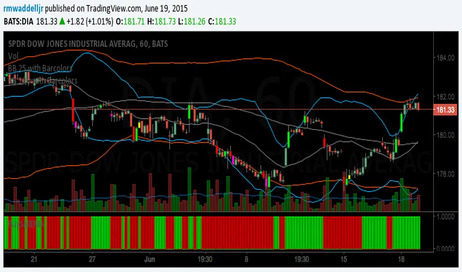
BB 100 with BarcolorsI cleaned up the highlight barcolor to reflect red or lime depending if it closed > or < the open.
The description is in the code. you want to catch bounces off the 25 (upper or lower) and 100 (upper or lower).
Works well on the hourly and 30 min charts. Haven't tested it beyond that. Haven't tested Forex, just equities.

EMA Keltner Channel 1D100/200 EMAs, along with Keltner Bands based off them. Colors correspond to actions you should be ready to take in the area. Use to set macro mindset.
Uses the security function to display only the 1D values.
Red= Bad
Orange = Not as Bad, but still Bad.
Yellow = Warning, might also be Bad.
Purple = Dip a toe in.
Blue = Give it a shot but have a little caution.
Green = It's second mortgage time.
BE-Volume Footprint & Pressure Candles█ Overview:
BE-Volume Footprint & Pressure Candles, is an indicator which is preliminarily designed to analyze the supply and demand patterns based on Rally Base Rally (RBR), Drop Base Drop (DBD), Drop Base Rally (DBR) & Rally Base Drop (RBD) concepts in conjunction to volume pressure. Understanding these concepts are crucial. Let's break down why the "Base" is you Best friend in this context.
Commonness in RBR, DBD, DBR, RBD patterns ?
There is an impulse price movement at first, be it rally (price moving up) or the Drop (price moving down), followed by a period of consolidation which is referred as "BASE" and later with another impulse move of price (Rally or Drop).
Why is the Base Important
1. Market Balance: Base represents a balance between buyers and sellers. This is where decisions are made.
2. Confirmation: It confirms the strength of previous impulse move which has happened.
Base & the Liquidity Play:
Supply & Demand Zone predict the presence of all large orders within the limits of the Base Zone. Price is expected to return to the zone to fill the unfilled orders placed by large players.
For the price to move in the intended direction Liquidity plays the major role. hence indicator aims to help traders in identifying those zones where liquidity exists and the volume pressure helps in confirming that liquidity is making its play.
Bottom pane in the below snapshots is a visual representation of Buyers volume pressure (Green Line & the Green filled area) making the price move upwards vs Sellers volume pressure (Red Line & the Red filled area) making the price move downwards.
Top pane in the below snapshots is a visual representation on the pattern identification (Blue marked zone & the Blue line referred as Liquidity level)
Bullish Pressure On Buy Liquidity:
Bearish Pressure On Sell Liquidity:
█ How It Works:
1. Indicator computes technical & mathematical operations such as ATR, delta of Highs & Lows of the candle and Candle ranges to identify the patterns and marks the liquidity lines accordingly.
2. Indicator then waits for price to return to the liquidity levels and checks if Directional volume pressure to flow-in while the prices hover near the Liquidity zones.
3. Once the Volume pressure is evident, loop in to the ride.
█ When It wont Work:
When there no sufficient Liquidity or sustained Opposite volume pressure, trades are expected to fail.
█ Limitations:
Works only on the scripts which has volume info. Relays on LTF candles to determine intra-bar volumes. Hence, Use on TF greater than 1 min and lesser than 15 min.
█ Indicator Features:
1. StrictEntries: employs' tighter rules (rather most significant setups) on the directional volume pressure applied for the price to move. If unchecked, liberal rules applied on the directional volume pressure leading to more setups being identified.
2. Setup Confirmation period: Indicates Waiting period to analyze the directional volume pressure. Early (lesser wait period) is Risky and Late (longer wait period) is too late for the
ride. Find the quant based on the accuracy of the setup provided in the bottom right table.
3. Algo Enabled with Place Holders:
Indicator is equipped with algo alerts, supported with necessary placeholders to trade any instrument like stock, options etc.
Accepted PlaceHolders (Case Sensitive!!)
1. {{ticker}}-->InstrumentName
2. {{datetime}}-->Date & Time Of Order Placement
3. {{close}}-->LTP Price of Script
4. {{TD}}-->Current Level:
Note: Negative Numbers for Short Setup
5. {{EN}} {{SL}} {{TGT}} {{T1}} {{T2}} --> Trade Levels
6. {{Qty}} {{Qty*x}} --> Qty -> Trade Qty mapped in Settings. Replace x with actual number of your choice for the multiplier
7. {{BS}}-->Based on the Direction of Trade Output shall be with B or S (B == Long Trade & S == Short Trade)
8. {{BUYSELL}}-->Based on the Direction of Trade Output shall be with BUY or SELL (BUY == Long Trade & SELL == Short Trade)
9. {{IBUYSELL}}-->Based on the Direction of Trade Output shall be with BUY or SELL (BUY == SHORT Trade & SELL == LONG Trade)
Dynamic Alerts:
10. { {100R0} }-->Dynamic Place Holder 100 Refers to Strike Difference and Zero refers to ATM
11. { {100R-1} }-->Dynamic Place Holder 100 Refers to Strike Difference and -1 refers to
ATM - 100 strike
12. { {50R2} }-->Dynamic Place Holder 50 Refers to Strike Difference and 2 refers to
ATM + (2 * 50 = 100) strike
13. { {"ddMMyy", 0} }-->Dynamically Picks today date in the specified format.
14. { {"ddMMyy", n} }-->replace n with actual number of your choice to Pick date post today date in the specified format.
15. { {"ddMMyy", "MON"} }-->dynamically pick Monday date (coming Monday, if today is not Monday)
Note. for the 2nd Param-->you can choose to specify either Number OR any letter from =>
16. {{CEPE}} {{ICEPE}} {{CP}} {{ICP}} -> Dynamic Option Side CE or C refers to Calls and PE or P refers to Puts. If "I" is used in PlaceHolder text, On long entries PUTs shall be used
Indicator is equipped with customizable Trade & Risk management settings like multiple Take profit levels, Trailing SL.

Price vs SMAThis indicator displays the current price in percentage terms, indicating whether it is above or below a selected simple moving average (SMA). It’s designed to be clean and minimal, with the option to display a brief sentence on the chart for added clarity.
The script calculates the distance between the current price and a chosen simple moving average (SMA) and expresses that distance as a percentage. By default, it uses the 200-period SMA, but you can adjust the length to any value, such as 50 or 100, depending on your trading style. A positive percentage means price is trading above the SMA, while a negative percentage means it is below.
The percentage difference is rounded to whole numbers and can be displayed directly in the chart legend if the “Indicator values” box is checked in the TradingView settings. This keeps the chart clean while still providing at-a-glance information about the price relative to your selected moving average.
For extra clarity, the script also includes an option to display a short sentence on the chart itself. This sentence will read “Price is x% above SMA” in green when price is above the SMA, or “Price is x% below SMA” in red when price is below. This visual cue makes it easy to interpret the relationship between price and the moving average without adding clutter.

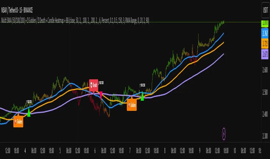
Multi SMA + Golden/Death + Heatmap + BB**Multi SMA (50/100/200) + Golden/Death + Candle Heatmap + BB**
A practical trend toolkit that blends classic 50/100/200 SMAs with clear crossover labels, special 🚀 Golden / 💀 Death Cross markers, and a readable candle heatmap based on a dynamic regression midline and volatility bands. Optional Bollinger Bands are included for context.
* See trend direction at a glance with SMAs.
* Get minimal, de-cluttered labels on important crosses (50↔100, 50↔200, 100↔200).
* Highlight big regime shifts with special Golden/Death tags.
* Read momentum and volatility with the candle heatmap.
* Add Bollinger Bands if you want classic mean-reversion context.
Designed to be lightweight, non-repainting on confirmed bars, and flexible across timeframes.
# What This Indicator Does (plain English)
* **Tracks trend** using **SMA 50/100/200** and lets you optionally compute each SMA on a higher or different timeframe (HTF-safe, no lookahead).
* **Prints labels** when SMAs cross each other (up or down). You can force signals only after bar close to avoid repaint.
* **Marks Golden/Death Crosses** (50 over/under 200) with special labels so major regime changes stand out.
* **Colors candles** with a **heatmap** built from a regression midline and volatility bands—greenish above, reddish below, with a smooth gradient.
* **Optionally shows Bollinger Bands** (basis SMA + stdev bands) and fills the area between them.
* **Includes alert conditions** for Golden and Death Cross so you can automate notifications.
---
# Settings — Simple Explanations
## Source
* **Source**: Price source used to calculate SMAs and Bollinger basis. Default: `close`.
## SMA 50
* **Show 50**: Turn the SMA(50) line on/off.
* **Length 50**: How many bars to average. Lower = faster but noisier.
* **Color 50** / **Width 50**: Visual style.
* **Timeframe 50**: Optional alternate timeframe for SMA(50). Leave empty to use the chart timeframe.
## SMA 100
* **Show 100**: Turn the SMA(100) line on/off.
* **Length 100**: Bars used for the mid-term trend.
* **Color 100** / **Width 100**: Visual style.
* **Timeframe 100**: Optional alternate timeframe for SMA(100).
## SMA 200
* **Show 200**: Turn the SMA(200) line on/off.
* **Length 200**: Bars used for the long-term trend.
* **Color 200** / **Width 200**: Visual style.
* **Timeframe 200**: Optional alternate timeframe for SMA(200).
## Signals (crossover labels)
* **Show crossover signals**: Prints triangle labels on SMA crosses (50↔100, 50↔200, 100↔200).
* **Wait for bar close (confirmed)**: If ON, signals only appear after the candle closes (reduces repaint).
* **Min bars between same-pair signals**: Minimum spacing to avoid duplicate labels from the same SMA pair too often.
* **Trend filter (buy: 50>100>200, sell: 50<100<200)**: Only show bullish labels when SMAs are stacked bullish (50 above 100 above 200), and only show bearish labels when stacked bearish.
### Label Offset
* **Offset mode**: Choose how to push labels away from price:
* **Percent**: Offset is a % of price.
* **ATR x**: Offset is ATR(14) × multiplier.
* **Percent of price (%)**: Used when mode = Percent.
* **ATR multiplier (for ‘ATR x’)**: Used when mode = ATR x.
### Label Colors
* **Bull color** / **Bear color**: Background of triangle labels.
* **Bull label text color** / **Bear label text color**: Text color inside the triangles.
## Golden / Death Cross
* **Show 🚀 Golden Cross (50↑200)**: Show a special “Golden” label when SMA50 crosses above SMA200.
* **Golden label color** / **Golden text color**: Styling for Golden label.
* **Show 💀 Death Cross (50↓200)**: Show a special “Death” label when SMA50 crosses below SMA200.
* **Death label color** / **Death text color**: Styling for Death label.
## Candle Heatmap
* **Enable heatmap candle colors**: Turns the heatmap on/off.
* **Length**: Lookback for the regression midline and volatility measure.
* **Deviation Multiplier**: Band width around the midline (bigger = wider).
* **Volatility basis**:
* **RMA Range** (smoothed high-low range)
* **Stdev** (standard deviation of close)
* **Upper/Middle/Lower color**: Gradient colors for the heatmap.
* **Heatmap transparency (0..100)**: 0 = solid, 100 = invisible.
* **Force override base candles**: Repaint base candles so heatmap stays visible even if your chart has custom coloring.
## Bollinger Bands (optional)
* **Show Bollinger Bands**: Toggle the overlay on/off.
* **Length**: Basis SMA length.
* **StdDev Multiplier**: Distance of bands from the basis in standard deviations.
* **Basis color** / **Band color**: Line colors for basis and bands.
* **Bands fill transparency**: Opacity of the fill between upper/lower bands.
---
# Features & How It Works
## 1) HTF-Safe SMAs
Each SMA can be calculated on the chart timeframe or a higher/different timeframe you choose. The script pulls HTF values **without lookahead** (non-repainting on confirmed bars).
## 2) Crossover Labels (Three Pairs)
* **50↔100**, **50↔200**, **100↔200**:
* **Triangle Up** label when the first SMA crosses **above** the second.
* **Triangle Down** label when it crosses **below**.
* Optional **Trend Filter** ensures only signals aligned with the overall stack (50>100>200 for bullish, 50<100<200 for bearish).
* **Debounce** spacing avoids repeated labels for the same pair too close together.
## 3) Golden / Death Cross Highlights
* **🚀 Golden Cross**: SMA50 crosses **above** SMA200 (often a longer-term bullish regime shift).
* **💀 Death Cross**: SMA50 crosses **below** SMA200 (often a longer-term bearish regime shift).
* Separate styling so they stand out from regular cross labels.
## 4) Candle Heatmap
* Builds a **regression midline** with **volatility bands**; colors candles by their position inside that channel.
* Smooth gradient: lower side → reddish, mid → yellowish, upper side → greenish.
* Helps you see momentum and “where price sits” relative to a dynamic channel.
## 5) Bollinger Bands (Optional)
* Classic **basis SMA** ± **StdDev** bands.
* Light visual context for mean-reversion and volatility expansion.
## 6) Alerts
* **Golden Cross**: `🚀 GOLDEN CROSS: SMA 50 crossed ABOVE SMA 200`
* **Death Cross**: `💀 DEATH CROSS: SMA 50 crossed BELOW SMA 200`
Add these to your alerts to get notified automatically.
---
# Tips & Notes
* For fewer false positives, keep **“Wait for bar close”** ON, especially on lower timeframes.
* Use the **Trend Filter** to align signals with the broader stack and cut noise.
* For HTF context, set **Timeframe 50/100/200** to higher frames (e.g., H1/H4/D) while you trade on a lower frame.
* Heatmap “Length” and “Deviation Multiplier” control smoothness and channel width—tune for your asset’s volatility.
Markov Chain [3D] | FractalystWhat exactly is a Markov Chain?
This indicator uses a Markov Chain model to analyze, quantify, and visualize the transitions between market regimes (Bull, Bear, Neutral) on your chart. It dynamically detects these regimes in real-time, calculates transition probabilities, and displays them as animated 3D spheres and arrows, giving traders intuitive insight into current and future market conditions.
How does a Markov Chain work, and how should I read this spheres-and-arrows diagram?
Think of three weather modes: Sunny, Rainy, Cloudy.
Each sphere is one mode. The loop on a sphere means “stay the same next step” (e.g., Sunny again tomorrow).
The arrows leaving a sphere show where things usually go next if they change (e.g., Sunny moving to Cloudy).
Some paths matter more than others. A more prominent loop means the current mode tends to persist. A more prominent outgoing arrow means a change to that destination is the usual next step.
Direction isn’t symmetric: moving Sunny→Cloudy can behave differently than Cloudy→Sunny.
Now relabel the spheres to markets: Bull, Bear, Neutral.
Spheres: market regimes (uptrend, downtrend, range).
Self‑loop: tendency for the current regime to continue on the next bar.
Arrows: the most common next regime if a switch happens.
How to read: Start at the sphere that matches current bar state. If the loop stands out, expect continuation. If one outgoing path stands out, that switch is the typical next step. Opposite directions can differ (Bear→Neutral doesn’t have to match Neutral→Bear).
What states and transitions are shown?
The three market states visualized are:
Bullish (Bull): Upward or strong-market regime.
Bearish (Bear): Downward or weak-market regime.
Neutral: Sideways or range-bound regime.
Bidirectional animated arrows and probability labels show how likely the market is to move from one regime to another (e.g., Bull → Bear or Neutral → Bull).
How does the regime detection system work?
You can use either built-in price returns (based on adaptive Z-score normalization) or supply three custom indicators (such as volume, oscillators, etc.).
Values are statistically normalized (Z-scored) over a configurable lookback period.
The normalized outputs are classified into Bull, Bear, or Neutral zones.
If using three indicators, their regime signals are averaged and smoothed for robustness.
How are transition probabilities calculated?
On every confirmed bar, the algorithm tracks the sequence of detected market states, then builds a rolling window of transitions.
The code maintains a transition count matrix for all regime pairs (e.g., Bull → Bear).
Transition probabilities are extracted for each possible state change using Laplace smoothing for numerical stability, and frequently updated in real-time.
What is unique about the visualization?
3D animated spheres represent each regime and change visually when active.
Animated, bidirectional arrows reveal transition probabilities and allow you to see both dominant and less likely regime flows.
Particles (moving dots) animate along the arrows, enhancing the perception of regime flow direction and speed.
All elements dynamically update with each new price bar, providing a live market map in an intuitive, engaging format.
Can I use custom indicators for regime classification?
Yes! Enable the "Custom Indicators" switch and select any three chart series as inputs. These will be normalized and combined (each with equal weight), broadening the regime classification beyond just price-based movement.
What does the “Lookback Period” control?
Lookback Period (default: 100) sets how much historical data builds the probability matrix. Shorter periods adapt faster to regime changes but may be noisier. Longer periods are more stable but slower to adapt.
How is this different from a Hidden Markov Model (HMM)?
It sets the window for both regime detection and probability calculations. Lower values make the system more reactive, but potentially noisier. Higher values smooth estimates and make the system more robust.
How is this Markov Chain different from a Hidden Markov Model (HMM)?
Markov Chain (as here): All market regimes (Bull, Bear, Neutral) are directly observable on the chart. The transition matrix is built from actual detected regimes, keeping the model simple and interpretable.
Hidden Markov Model: The actual regimes are unobservable ("hidden") and must be inferred from market output or indicator "emissions" using statistical learning algorithms. HMMs are more complex, can capture more subtle structure, but are harder to visualize and require additional machine learning steps for training.
A standard Markov Chain models transitions between observable states using a simple transition matrix, while a Hidden Markov Model assumes the true states are hidden (latent) and must be inferred from observable “emissions” like price or volume data. In practical terms, a Markov Chain is transparent and easier to implement and interpret; an HMM is more expressive but requires statistical inference to estimate hidden states from data.
Markov Chain: states are observable; you directly count or estimate transition probabilities between visible states. This makes it simpler, faster, and easier to validate and tune.
HMM: states are hidden; you only observe emissions generated by those latent states. Learning involves machine learning/statistical algorithms (commonly Baum–Welch/EM for training and Viterbi for decoding) to infer both the transition dynamics and the most likely hidden state sequence from data.
How does the indicator avoid “repainting” or look-ahead bias?
All regime changes and matrix updates happen only on confirmed (closed) bars, so no future data is leaked, ensuring reliable real-time operation.
Are there practical tuning tips?
Tune the Lookback Period for your asset/timeframe: shorter for fast markets, longer for stability.
Use custom indicators if your asset has unique regime drivers.
Watch for rapid changes in transition probabilities as early warning of a possible regime shift.
Who is this indicator for?
Quants and quantitative researchers exploring probabilistic market modeling, especially those interested in regime-switching dynamics and Markov models.
Programmers and system developers who need a probabilistic regime filter for systematic and algorithmic backtesting:
The Markov Chain indicator is ideally suited for programmatic integration via its bias output (1 = Bull, 0 = Neutral, -1 = Bear).
Although the visualization is engaging, the core output is designed for automated, rules-based workflows—not for discretionary/manual trading decisions.
Developers can connect the indicator’s output directly to their Pine Script logic (using input.source()), allowing rapid and robust backtesting of regime-based strategies.
It acts as a plug-and-play regime filter: simply plug the bias output into your entry/exit logic, and you have a scientifically robust, probabilistically-derived signal for filtering, timing, position sizing, or risk regimes.
The MC's output is intentionally "trinary" (1/0/-1), focusing on clear regime states for unambiguous decision-making in code. If you require nuanced, multi-probability or soft-label state vectors, consider expanding the indicator or stacking it with a probability-weighted logic layer in your scripting.
Because it avoids subjectivity, this approach is optimal for systematic quants, algo developers building backtested, repeatable strategies based on probabilistic regime analysis.
What's the mathematical foundation behind this?
The mathematical foundation behind this Markov Chain indicator—and probabilistic regime detection in finance—draws from two principal models: the (standard) Markov Chain and the Hidden Markov Model (HMM).
How to use this indicator programmatically?
The Markov Chain indicator automatically exports a bias value (+1 for Bullish, -1 for Bearish, 0 for Neutral) as a plot visible in the Data Window. This allows you to integrate its regime signal into your own scripts and strategies for backtesting, automation, or live trading.
Step-by-Step Integration with Pine Script (input.source)
Add the Markov Chain indicator to your chart.
This must be done first, since your custom script will "pull" the bias signal from the indicator's plot.
In your strategy, create an input using input.source()
Example:
//@version=5
strategy("MC Bias Strategy Example")
mcBias = input.source(close, "MC Bias Source")
After saving, go to your script’s settings. For the “MC Bias Source” input, select the plot/output of the Markov Chain indicator (typically its bias plot).
Use the bias in your trading logic
Example (long only on Bull, flat otherwise):
if mcBias == 1
strategy.entry("Long", strategy.long)
else
strategy.close("Long")
For more advanced workflows, combine mcBias with additional filters or trailing stops.
How does this work behind-the-scenes?
TradingView’s input.source() lets you use any plot from another indicator as a real-time, “live” data feed in your own script (source).
The selected bias signal is available to your Pine code as a variable, enabling logical decisions based on regime (trend-following, mean-reversion, etc.).
This enables powerful strategy modularity : decouple regime detection from entry/exit logic, allowing fast experimentation without rewriting core signal code.
Integrating 45+ Indicators with Your Markov Chain — How & Why
The Enhanced Custom Indicators Export script exports a massive suite of over 45 technical indicators—ranging from classic momentum (RSI, MACD, Stochastic, etc.) to trend, volume, volatility, and oscillator tools—all pre-calculated, centered/scaled, and available as plots.
// Enhanced Custom Indicators Export - 45 Technical Indicators
// Comprehensive technical analysis suite for advanced market regime detection
//@version=6
indicator('Enhanced Custom Indicators Export | Fractalyst', shorttitle='Enhanced CI Export', overlay=false, scale=scale.right, max_labels_count=500, max_lines_count=500)
// |----- Input Parameters -----| //
momentum_group = "Momentum Indicators"
trend_group = "Trend Indicators"
volume_group = "Volume Indicators"
volatility_group = "Volatility Indicators"
oscillator_group = "Oscillator Indicators"
display_group = "Display Settings"
// Common lengths
length_14 = input.int(14, "Standard Length (14)", minval=1, maxval=100, group=momentum_group)
length_20 = input.int(20, "Medium Length (20)", minval=1, maxval=200, group=trend_group)
length_50 = input.int(50, "Long Length (50)", minval=1, maxval=200, group=trend_group)
// Display options
show_table = input.bool(true, "Show Values Table", group=display_group)
table_size = input.string("Small", "Table Size", options= , group=display_group)
// |----- MOMENTUM INDICATORS (15 indicators) -----| //
// 1. RSI (Relative Strength Index)
rsi_14 = ta.rsi(close, length_14)
rsi_centered = rsi_14 - 50
// 2. Stochastic Oscillator
stoch_k = ta.stoch(close, high, low, length_14)
stoch_d = ta.sma(stoch_k, 3)
stoch_centered = stoch_k - 50
// 3. Williams %R
williams_r = ta.stoch(close, high, low, length_14) - 100
// 4. MACD (Moving Average Convergence Divergence)
= ta.macd(close, 12, 26, 9)
// 5. Momentum (Rate of Change)
momentum = ta.mom(close, length_14)
momentum_pct = (momentum / close ) * 100
// 6. Rate of Change (ROC)
roc = ta.roc(close, length_14)
// 7. Commodity Channel Index (CCI)
cci = ta.cci(close, length_20)
// 8. Money Flow Index (MFI)
mfi = ta.mfi(close, length_14)
mfi_centered = mfi - 50
// 9. Awesome Oscillator (AO)
ao = ta.sma(hl2, 5) - ta.sma(hl2, 34)
// 10. Accelerator Oscillator (AC)
ac = ao - ta.sma(ao, 5)
// 11. Chande Momentum Oscillator (CMO)
cmo = ta.cmo(close, length_14)
// 12. Detrended Price Oscillator (DPO)
dpo = close - ta.sma(close, length_20)
// 13. Price Oscillator (PPO)
ppo = ta.sma(close, 12) - ta.sma(close, 26)
ppo_pct = (ppo / ta.sma(close, 26)) * 100
// 14. TRIX
trix_ema1 = ta.ema(close, length_14)
trix_ema2 = ta.ema(trix_ema1, length_14)
trix_ema3 = ta.ema(trix_ema2, length_14)
trix = ta.roc(trix_ema3, 1) * 10000
// 15. Klinger Oscillator
klinger = ta.ema(volume * (high + low + close) / 3, 34) - ta.ema(volume * (high + low + close) / 3, 55)
// 16. Fisher Transform
fisher_hl2 = 0.5 * (hl2 - ta.lowest(hl2, 10)) / (ta.highest(hl2, 10) - ta.lowest(hl2, 10)) - 0.25
fisher = 0.5 * math.log((1 + fisher_hl2) / (1 - fisher_hl2))
// 17. Stochastic RSI
stoch_rsi = ta.stoch(rsi_14, rsi_14, rsi_14, length_14)
stoch_rsi_centered = stoch_rsi - 50
// 18. Relative Vigor Index (RVI)
rvi_num = ta.swma(close - open)
rvi_den = ta.swma(high - low)
rvi = rvi_den != 0 ? rvi_num / rvi_den : 0
// 19. Balance of Power (BOP)
bop = (close - open) / (high - low)
// |----- TREND INDICATORS (10 indicators) -----| //
// 20. Simple Moving Average Momentum
sma_20 = ta.sma(close, length_20)
sma_momentum = ((close - sma_20) / sma_20) * 100
// 21. Exponential Moving Average Momentum
ema_20 = ta.ema(close, length_20)
ema_momentum = ((close - ema_20) / ema_20) * 100
// 22. Parabolic SAR
sar = ta.sar(0.02, 0.02, 0.2)
sar_trend = close > sar ? 1 : -1
// 23. Linear Regression Slope
lr_slope = ta.linreg(close, length_20, 0) - ta.linreg(close, length_20, 1)
// 24. Moving Average Convergence (MAC)
mac = ta.sma(close, 10) - ta.sma(close, 30)
// 25. Trend Intensity Index (TII)
tii_sum = 0.0
for i = 1 to length_20
tii_sum += close > close ? 1 : 0
tii = (tii_sum / length_20) * 100
// 26. Ichimoku Cloud Components
ichimoku_tenkan = (ta.highest(high, 9) + ta.lowest(low, 9)) / 2
ichimoku_kijun = (ta.highest(high, 26) + ta.lowest(low, 26)) / 2
ichimoku_signal = ichimoku_tenkan > ichimoku_kijun ? 1 : -1
// 27. MESA Adaptive Moving Average (MAMA)
mama_alpha = 2.0 / (length_20 + 1)
mama = ta.ema(close, length_20)
mama_momentum = ((close - mama) / mama) * 100
// 28. Zero Lag Exponential Moving Average (ZLEMA)
zlema_lag = math.round((length_20 - 1) / 2)
zlema_data = close + (close - close )
zlema = ta.ema(zlema_data, length_20)
zlema_momentum = ((close - zlema) / zlema) * 100
// |----- VOLUME INDICATORS (6 indicators) -----| //
// 29. On-Balance Volume (OBV)
obv = ta.obv
// 30. Volume Rate of Change (VROC)
vroc = ta.roc(volume, length_14)
// 31. Price Volume Trend (PVT)
pvt = ta.pvt
// 32. Negative Volume Index (NVI)
nvi = 0.0
nvi := volume < volume ? nvi + ((close - close ) / close ) * nvi : nvi
// 33. Positive Volume Index (PVI)
pvi = 0.0
pvi := volume > volume ? pvi + ((close - close ) / close ) * pvi : pvi
// 34. Volume Oscillator
vol_osc = ta.sma(volume, 5) - ta.sma(volume, 10)
// 35. Ease of Movement (EOM)
eom_distance = high - low
eom_box_height = volume / 1000000
eom = eom_box_height != 0 ? eom_distance / eom_box_height : 0
eom_sma = ta.sma(eom, length_14)
// 36. Force Index
force_index = volume * (close - close )
force_index_sma = ta.sma(force_index, length_14)
// |----- VOLATILITY INDICATORS (10 indicators) -----| //
// 37. Average True Range (ATR)
atr = ta.atr(length_14)
atr_pct = (atr / close) * 100
// 38. Bollinger Bands Position
bb_basis = ta.sma(close, length_20)
bb_dev = 2.0 * ta.stdev(close, length_20)
bb_upper = bb_basis + bb_dev
bb_lower = bb_basis - bb_dev
bb_position = bb_dev != 0 ? (close - bb_basis) / bb_dev : 0
bb_width = bb_dev != 0 ? (bb_upper - bb_lower) / bb_basis * 100 : 0
// 39. Keltner Channels Position
kc_basis = ta.ema(close, length_20)
kc_range = ta.ema(ta.tr, length_20)
kc_upper = kc_basis + (2.0 * kc_range)
kc_lower = kc_basis - (2.0 * kc_range)
kc_position = kc_range != 0 ? (close - kc_basis) / kc_range : 0
// 40. Donchian Channels Position
dc_upper = ta.highest(high, length_20)
dc_lower = ta.lowest(low, length_20)
dc_basis = (dc_upper + dc_lower) / 2
dc_position = (dc_upper - dc_lower) != 0 ? (close - dc_basis) / (dc_upper - dc_lower) : 0
// 41. Standard Deviation
std_dev = ta.stdev(close, length_20)
std_dev_pct = (std_dev / close) * 100
// 42. Relative Volatility Index (RVI)
rvi_up = ta.stdev(close > close ? close : 0, length_14)
rvi_down = ta.stdev(close < close ? close : 0, length_14)
rvi_total = rvi_up + rvi_down
rvi_volatility = rvi_total != 0 ? (rvi_up / rvi_total) * 100 : 50
// 43. Historical Volatility
hv_returns = math.log(close / close )
hv = ta.stdev(hv_returns, length_20) * math.sqrt(252) * 100
// 44. Garman-Klass Volatility
gk_vol = math.log(high/low) * math.log(high/low) - (2*math.log(2)-1) * math.log(close/open) * math.log(close/open)
gk_volatility = math.sqrt(ta.sma(gk_vol, length_20)) * 100
// 45. Parkinson Volatility
park_vol = math.log(high/low) * math.log(high/low)
parkinson = math.sqrt(ta.sma(park_vol, length_20) / (4 * math.log(2))) * 100
// 46. Rogers-Satchell Volatility
rs_vol = math.log(high/close) * math.log(high/open) + math.log(low/close) * math.log(low/open)
rogers_satchell = math.sqrt(ta.sma(rs_vol, length_20)) * 100
// |----- OSCILLATOR INDICATORS (5 indicators) -----| //
// 47. Elder Ray Index
elder_bull = high - ta.ema(close, 13)
elder_bear = low - ta.ema(close, 13)
elder_power = elder_bull + elder_bear
// 48. Schaff Trend Cycle (STC)
stc_macd = ta.ema(close, 23) - ta.ema(close, 50)
stc_k = ta.stoch(stc_macd, stc_macd, stc_macd, 10)
stc_d = ta.ema(stc_k, 3)
stc = ta.stoch(stc_d, stc_d, stc_d, 10)
// 49. Coppock Curve
coppock_roc1 = ta.roc(close, 14)
coppock_roc2 = ta.roc(close, 11)
coppock = ta.wma(coppock_roc1 + coppock_roc2, 10)
// 50. Know Sure Thing (KST)
kst_roc1 = ta.roc(close, 10)
kst_roc2 = ta.roc(close, 15)
kst_roc3 = ta.roc(close, 20)
kst_roc4 = ta.roc(close, 30)
kst = ta.sma(kst_roc1, 10) + 2*ta.sma(kst_roc2, 10) + 3*ta.sma(kst_roc3, 10) + 4*ta.sma(kst_roc4, 15)
// 51. Percentage Price Oscillator (PPO)
ppo_line = ((ta.ema(close, 12) - ta.ema(close, 26)) / ta.ema(close, 26)) * 100
ppo_signal = ta.ema(ppo_line, 9)
ppo_histogram = ppo_line - ppo_signal
// |----- PLOT MAIN INDICATORS -----| //
// Plot key momentum indicators
plot(rsi_centered, title="01_RSI_Centered", color=color.purple, linewidth=1)
plot(stoch_centered, title="02_Stoch_Centered", color=color.blue, linewidth=1)
plot(williams_r, title="03_Williams_R", color=color.red, linewidth=1)
plot(macd_histogram, title="04_MACD_Histogram", color=color.orange, linewidth=1)
plot(cci, title="05_CCI", color=color.green, linewidth=1)
// Plot trend indicators
plot(sma_momentum, title="06_SMA_Momentum", color=color.navy, linewidth=1)
plot(ema_momentum, title="07_EMA_Momentum", color=color.maroon, linewidth=1)
plot(sar_trend, title="08_SAR_Trend", color=color.teal, linewidth=1)
plot(lr_slope, title="09_LR_Slope", color=color.lime, linewidth=1)
plot(mac, title="10_MAC", color=color.fuchsia, linewidth=1)
// Plot volatility indicators
plot(atr_pct, title="11_ATR_Pct", color=color.yellow, linewidth=1)
plot(bb_position, title="12_BB_Position", color=color.aqua, linewidth=1)
plot(kc_position, title="13_KC_Position", color=color.olive, linewidth=1)
plot(std_dev_pct, title="14_StdDev_Pct", color=color.silver, linewidth=1)
plot(bb_width, title="15_BB_Width", color=color.gray, linewidth=1)
// Plot volume indicators
plot(vroc, title="16_VROC", color=color.blue, linewidth=1)
plot(eom_sma, title="17_EOM", color=color.red, linewidth=1)
plot(vol_osc, title="18_Vol_Osc", color=color.green, linewidth=1)
plot(force_index_sma, title="19_Force_Index", color=color.orange, linewidth=1)
plot(obv, title="20_OBV", color=color.purple, linewidth=1)
// Plot additional oscillators
plot(ao, title="21_Awesome_Osc", color=color.navy, linewidth=1)
plot(cmo, title="22_CMO", color=color.maroon, linewidth=1)
plot(dpo, title="23_DPO", color=color.teal, linewidth=1)
plot(trix, title="24_TRIX", color=color.lime, linewidth=1)
plot(fisher, title="25_Fisher", color=color.fuchsia, linewidth=1)
// Plot more momentum indicators
plot(mfi_centered, title="26_MFI_Centered", color=color.yellow, linewidth=1)
plot(ac, title="27_AC", color=color.aqua, linewidth=1)
plot(ppo_pct, title="28_PPO_Pct", color=color.olive, linewidth=1)
plot(stoch_rsi_centered, title="29_StochRSI_Centered", color=color.silver, linewidth=1)
plot(klinger, title="30_Klinger", color=color.gray, linewidth=1)
// Plot trend continuation
plot(tii, title="31_TII", color=color.blue, linewidth=1)
plot(ichimoku_signal, title="32_Ichimoku_Signal", color=color.red, linewidth=1)
plot(mama_momentum, title="33_MAMA_Momentum", color=color.green, linewidth=1)
plot(zlema_momentum, title="34_ZLEMA_Momentum", color=color.orange, linewidth=1)
plot(bop, title="35_BOP", color=color.purple, linewidth=1)
// Plot volume continuation
plot(nvi, title="36_NVI", color=color.navy, linewidth=1)
plot(pvi, title="37_PVI", color=color.maroon, linewidth=1)
plot(momentum_pct, title="38_Momentum_Pct", color=color.teal, linewidth=1)
plot(roc, title="39_ROC", color=color.lime, linewidth=1)
plot(rvi, title="40_RVI", color=color.fuchsia, linewidth=1)
// Plot volatility continuation
plot(dc_position, title="41_DC_Position", color=color.yellow, linewidth=1)
plot(rvi_volatility, title="42_RVI_Volatility", color=color.aqua, linewidth=1)
plot(hv, title="43_Historical_Vol", color=color.olive, linewidth=1)
plot(gk_volatility, title="44_GK_Volatility", color=color.silver, linewidth=1)
plot(parkinson, title="45_Parkinson_Vol", color=color.gray, linewidth=1)
// Plot final oscillators
plot(rogers_satchell, title="46_RS_Volatility", color=color.blue, linewidth=1)
plot(elder_power, title="47_Elder_Power", color=color.red, linewidth=1)
plot(stc, title="48_STC", color=color.green, linewidth=1)
plot(coppock, title="49_Coppock", color=color.orange, linewidth=1)
plot(kst, title="50_KST", color=color.purple, linewidth=1)
// Plot final indicators
plot(ppo_histogram, title="51_PPO_Histogram", color=color.navy, linewidth=1)
plot(pvt, title="52_PVT", color=color.maroon, linewidth=1)
// |----- Reference Lines -----| //
hline(0, "Zero Line", color=color.gray, linestyle=hline.style_dashed, linewidth=1)
hline(50, "Midline", color=color.gray, linestyle=hline.style_dotted, linewidth=1)
hline(-50, "Lower Midline", color=color.gray, linestyle=hline.style_dotted, linewidth=1)
hline(25, "Upper Threshold", color=color.gray, linestyle=hline.style_dotted, linewidth=1)
hline(-25, "Lower Threshold", color=color.gray, linestyle=hline.style_dotted, linewidth=1)
// |----- Enhanced Information Table -----| //
if show_table and barstate.islast
table_position = position.top_right
table_text_size = table_size == "Tiny" ? size.tiny : table_size == "Small" ? size.small : size.normal
var table info_table = table.new(table_position, 3, 18, bgcolor=color.new(color.white, 85), border_width=1, border_color=color.gray)
// Headers
table.cell(info_table, 0, 0, 'Category', text_color=color.black, text_size=table_text_size, bgcolor=color.new(color.blue, 70))
table.cell(info_table, 1, 0, 'Indicator', text_color=color.black, text_size=table_text_size, bgcolor=color.new(color.blue, 70))
table.cell(info_table, 2, 0, 'Value', text_color=color.black, text_size=table_text_size, bgcolor=color.new(color.blue, 70))
// Key Momentum Indicators
table.cell(info_table, 0, 1, 'MOMENTUM', text_color=color.purple, text_size=table_text_size, bgcolor=color.new(color.purple, 90))
table.cell(info_table, 1, 1, 'RSI Centered', text_color=color.purple, text_size=table_text_size)
table.cell(info_table, 2, 1, str.tostring(rsi_centered, '0.00'), text_color=color.purple, text_size=table_text_size)
table.cell(info_table, 0, 2, '', text_color=color.blue, text_size=table_text_size)
table.cell(info_table, 1, 2, 'Stoch Centered', text_color=color.blue, text_size=table_text_size)
table.cell(info_table, 2, 2, str.tostring(stoch_centered, '0.00'), text_color=color.blue, text_size=table_text_size)
table.cell(info_table, 0, 3, '', text_color=color.red, text_size=table_text_size)
table.cell(info_table, 1, 3, 'Williams %R', text_color=color.red, text_size=table_text_size)
table.cell(info_table, 2, 3, str.tostring(williams_r, '0.00'), text_color=color.red, text_size=table_text_size)
table.cell(info_table, 0, 4, '', text_color=color.orange, text_size=table_text_size)
table.cell(info_table, 1, 4, 'MACD Histogram', text_color=color.orange, text_size=table_text_size)
table.cell(info_table, 2, 4, str.tostring(macd_histogram, '0.000'), text_color=color.orange, text_size=table_text_size)
table.cell(info_table, 0, 5, '', text_color=color.green, text_size=table_text_size)
table.cell(info_table, 1, 5, 'CCI', text_color=color.green, text_size=table_text_size)
table.cell(info_table, 2, 5, str.tostring(cci, '0.00'), text_color=color.green, text_size=table_text_size)
// Key Trend Indicators
table.cell(info_table, 0, 6, 'TREND', text_color=color.navy, text_size=table_text_size, bgcolor=color.new(color.navy, 90))
table.cell(info_table, 1, 6, 'SMA Momentum %', text_color=color.navy, text_size=table_text_size)
table.cell(info_table, 2, 6, str.tostring(sma_momentum, '0.00'), text_color=color.navy, text_size=table_text_size)
table.cell(info_table, 0, 7, '', text_color=color.maroon, text_size=table_text_size)
table.cell(info_table, 1, 7, 'EMA Momentum %', text_color=color.maroon, text_size=table_text_size)
table.cell(info_table, 2, 7, str.tostring(ema_momentum, '0.00'), text_color=color.maroon, text_size=table_text_size)
table.cell(info_table, 0, 8, '', text_color=color.teal, text_size=table_text_size)
table.cell(info_table, 1, 8, 'SAR Trend', text_color=color.teal, text_size=table_text_size)
table.cell(info_table, 2, 8, str.tostring(sar_trend, '0'), text_color=color.teal, text_size=table_text_size)
table.cell(info_table, 0, 9, '', text_color=color.lime, text_size=table_text_size)
table.cell(info_table, 1, 9, 'Linear Regression', text_color=color.lime, text_size=table_text_size)
table.cell(info_table, 2, 9, str.tostring(lr_slope, '0.000'), text_color=color.lime, text_size=table_text_size)
// Key Volatility Indicators
table.cell(info_table, 0, 10, 'VOLATILITY', text_color=color.yellow, text_size=table_text_size, bgcolor=color.new(color.yellow, 90))
table.cell(info_table, 1, 10, 'ATR %', text_color=color.yellow, text_size=table_text_size)
table.cell(info_table, 2, 10, str.tostring(atr_pct, '0.00'), text_color=color.yellow, text_size=table_text_size)
table.cell(info_table, 0, 11, '', text_color=color.aqua, text_size=table_text_size)
table.cell(info_table, 1, 11, 'BB Position', text_color=color.aqua, text_size=table_text_size)
table.cell(info_table, 2, 11, str.tostring(bb_position, '0.00'), text_color=color.aqua, text_size=table_text_size)
table.cell(info_table, 0, 12, '', text_color=color.olive, text_size=table_text_size)
table.cell(info_table, 1, 12, 'KC Position', text_color=color.olive, text_size=table_text_size)
table.cell(info_table, 2, 12, str.tostring(kc_position, '0.00'), text_color=color.olive, text_size=table_text_size)
// Key Volume Indicators
table.cell(info_table, 0, 13, 'VOLUME', text_color=color.blue, text_size=table_text_size, bgcolor=color.new(color.blue, 90))
table.cell(info_table, 1, 13, 'Volume ROC', text_color=color.blue, text_size=table_text_size)
table.cell(info_table, 2, 13, str.tostring(vroc, '0.00'), text_color=color.blue, text_size=table_text_size)
table.cell(info_table, 0, 14, '', text_color=color.red, text_size=table_text_size)
table.cell(info_table, 1, 14, 'EOM', text_color=color.red, text_size=table_text_size)
table.cell(info_table, 2, 14, str.tostring(eom_sma, '0.000'), text_color=color.red, text_size=table_text_size)
// Key Oscillators
table.cell(info_table, 0, 15, 'OSCILLATORS', text_color=color.purple, text_size=table_text_size, bgcolor=color.new(color.purple, 90))
table.cell(info_table, 1, 15, 'Awesome Osc', text_color=color.blue, text_size=table_text_size)
table.cell(info_table, 2, 15, str.tostring(ao, '0.000'), text_color=color.blue, text_size=table_text_size)
table.cell(info_table, 0, 16, '', text_color=color.red, text_size=table_text_size)
table.cell(info_table, 1, 16, 'Fisher Transform', text_color=color.red, text_size=table_text_size)
table.cell(info_table, 2, 16, str.tostring(fisher, '0.000'), text_color=color.red, text_size=table_text_size)
// Summary Statistics
table.cell(info_table, 0, 17, 'SUMMARY', text_color=color.black, text_size=table_text_size, bgcolor=color.new(color.gray, 70))
table.cell(info_table, 1, 17, 'Total Indicators: 52', text_color=color.black, text_size=table_text_size)
regime_color = rsi_centered > 10 ? color.green : rsi_centered < -10 ? color.red : color.gray
regime_text = rsi_centered > 10 ? "BULLISH" : rsi_centered < -10 ? "BEARISH" : "NEUTRAL"
table.cell(info_table, 2, 17, regime_text, text_color=regime_color, text_size=table_text_size)
This makes it the perfect “indicator backbone” for quantitative and systematic traders who want to prototype, combine, and test new regime detection models—especially in combination with the Markov Chain indicator.
How to use this script with the Markov Chain for research and backtesting:
Add the Enhanced Indicator Export to your chart.
Every calculated indicator is available as an individual data stream.
Connect the indicator(s) you want as custom input(s) to the Markov Chain’s “Custom Indicators” option.
In the Markov Chain indicator’s settings, turn ON the custom indicator mode.
For each of the three custom indicator inputs, select the exported plot from the Enhanced Export script—the menu lists all 45+ signals by name.
This creates a powerful, modular regime-detection engine where you can mix-and-match momentum, trend, volume, or custom combinations for advanced filtering.
Backtest regime logic directly.
Once you’ve connected your chosen indicators, the Markov Chain script performs regime detection (Bull/Neutral/Bear) based on your selected features—not just price returns.
The regime detection is robust, automatically normalized (using Z-score), and outputs bias (1, -1, 0) for plug-and-play integration.
Export the regime bias for programmatic use.
As described above, use input.source() in your Pine Script strategy or system and link the bias output.
You can now filter signals, control trade direction/size, or design pairs-trading that respect true, indicator-driven market regimes.
With this framework, you’re not limited to static or simplistic regime filters. You can rigorously define, test, and refine what “market regime” means for your strategies—using the technical features that matter most to you.
Optimize your signal generation by backtesting across a universe of meaningful indicator blends.
Enhance risk management with objective, real-time regime boundaries.
Accelerate your research: iterate quickly, swap indicator components, and see results with minimal code changes.
Automate multi-asset or pairs-trading by integrating regime context directly into strategy logic.
Add both scripts to your chart, connect your preferred features, and start investigating your best regime-based trades—entirely within the TradingView ecosystem.
References & Further Reading
Ang, A., & Bekaert, G. (2002). “Regime Switches in Interest Rates.” Journal of Business & Economic Statistics, 20(2), 163–182.
Hamilton, J. D. (1989). “A New Approach to the Economic Analysis of Nonstationary Time Series and the Business Cycle.” Econometrica, 57(2), 357–384.
Markov, A. A. (1906). "Extension of the Limit Theorems of Probability Theory to a Sum of Variables Connected in a Chain." The Notes of the Imperial Academy of Sciences of St. Petersburg.
Guidolin, M., & Timmermann, A. (2007). “Asset Allocation under Multivariate Regime Switching.” Journal of Economic Dynamics and Control, 31(11), 3503–3544.
Murphy, J. J. (1999). Technical Analysis of the Financial Markets. New York Institute of Finance.
Brock, W., Lakonishok, J., & LeBaron, B. (1992). “Simple Technical Trading Rules and the Stochastic Properties of Stock Returns.” Journal of Finance, 47(5), 1731–1764.
Zucchini, W., MacDonald, I. L., & Langrock, R. (2017). Hidden Markov Models for Time Series: An Introduction Using R (2nd ed.). Chapman and Hall/CRC.
On Quantitative Finance and Markov Models:
Lo, A. W., & Hasanhodzic, J. (2009). The Heretics of Finance: Conversations with Leading Practitioners of Technical Analysis. Bloomberg Press.
Patterson, S. (2016). The Man Who Solved the Market: How Jim Simons Launched the Quant Revolution. Penguin Press.
TradingView Pine Script Documentation: www.tradingview.com
TradingView Blog: “Use an Input From Another Indicator With Your Strategy” www.tradingview.com
GeeksforGeeks: “What is the Difference Between Markov Chains and Hidden Markov Models?” www.geeksforgeeks.org
What makes this indicator original and unique?
- On‑chart, real‑time Markov. The chain is drawn directly on your chart. You see the current regime, its tendency to stay (self‑loop), and the usual next step (arrows) as bars confirm.
- Source‑agnostic by design. The engine runs on any series you select via input.source() — price, your own oscillator, a composite score, anything you compute in the script.
- Automatic normalization + regime mapping. Different inputs live on different scales. The script standardizes your chosen source and maps it into clear regimes (e.g., Bull / Bear / Neutral) without you micromanaging thresholds each time.
- Rolling, bar‑by‑bar learning. Transition tendencies are computed from a rolling window of confirmed bars. What you see is exactly what the market did in that window.
- Fast experimentation. Switch the source, adjust the window, and the Markov view updates instantly. It’s a rapid way to test ideas and feel regime persistence/switch behavior.
Integrate your own signals (using input.source())
- In settings, choose the Source . This is powered by input.source() .
- Feed it price, an indicator you compute inside the script, or a custom composite series.
- The script will automatically normalize that series and process it through the Markov engine, mapping it to regimes and updating the on‑chart spheres/arrows in real time.
Credits:
Deep gratitude to @RicardoSantos for both the foundational Markov chain processing engine and inspiring open-source contributions, which made advanced probabilistic market modeling accessible to the TradingView community.
Special thanks to @Alien_Algorithms for the innovative and visually stunning 3D sphere logic that powers the indicator’s animated, regime-based visualization.
Disclaimer
This tool summarizes recent behavior. It is not financial advice and not a guarantee of future results.

Real Woodies CCIAs always, this is not financial advice and use at your own risk. Trading is risky and can cost you significant sums of money if you are not careful. Make sure you always have a proper entry and exit plan that includes defining your risk before you enter a trade.
Ken Wood is a semi-famous trader that grew in popularity in the 1990s and early 2000s due to the establishment of one of the earliest trading forums online. This forum grew into "Woodie's CCI Club" due to Wood's love of his modified Commodity Channel Index (CCI) that he used extensively. From what I can tell, the website is still active and still follows the same core principles it did in the early days, the CCI is used for entries, range bars are used to help trader's cut down on the noise, and the optional addition of Woodie's Pivot Points can be used as further confirmation of support and resistance. This is my take on his famous "Woodie's CCI" that has become standard on many charting packages through the years, including a TradingView sponsored version as one of the many stock indicators provided by TradingView. Woodie has updated his CCI through the years to include several very cool additions outside of the standard CCI. I will have to say, I am a bit biased, but I think this is hands down one of the best indicators I have ever used, and I am far too young to have been part of the original CCI Club. Being a daytrader primarily, this fits right in my timeframe wheel house. Woodie designed this indicator to work on a day-trading time scale and he frequently uses this to trade futures and commodity contracts on the 30 minute, often even down to the one minute timeframe. This makes it unique in that it is probably one of the only daytrading-designed indicators out there that I am aware of that was not a popular indicator, like the MACD or RSI, that was just adopted by daytraders.
The CCI was originally created by Donald Lambert in 1980. Over time, it has become an extremely popular house-hold indicator, like the Stochastics, RSI, or MACD. However, like the RSI and Stochastics, there are extensive debates on how the CCI is actually meant to be used. Some trade it like a reversal indicator, where values greater than 100 or less than -100 are considered overbought or oversold, respectively. Others trade it like a typical zero-line cross indicator, where once the value goes above or below the zero-line, a trade should be considered in that direction. Lastly, some treat it as strictly a momentum indicator, where values greater than 100 or less than -100 are seen as strong momentum moves and when these values are reached, a new strong trend is establishing in the direction of the move. The CCI itself is nothing fancy, it just visualizes the distance of the closing price away from a user-defined SMA value and plots it as a line. However, Woodie's CCI takes this simple concept and adds to it with an indicator with 5 pieces to it designed to help the trader enter into the highest probability setups. Bear with me, it initially looks super complicated, but I promise it is pretty straight-forward and a fun indicator to use.
1) The CCI Histogram. This is your standard CCI value that you would find on the normal CCI. Woodie's CCI uses a value of 14 for most trades and a value of 20 when the timeframe is equal to or greater than 30minutes. I personally use this as a 20-period CCI on all time frames, simply for the fact that the 20 SMA is a very popular moving average and I want to know what the crowd is doing. This is your coloured histogram with 4 colours. A gray colouring is for any bars above or below the zero line for 1-4 bars. A yellow bar is a "trend bar", where the long period CCI has been above/below the zero line for 5 consecutive bars, indicating that a trend in the current direction has been established. Blue bars above and red bars below are simply 6+n number of bars above or below the zero line confirming trend. These are used for the Zero-Line Reject Trade (explained below). The CCI Histogram has a matching long-period CCI line that is painted the same colour as the histogram, it is the same thing but is used just to outline the Histogram a bit better.
2) The CCI Turbo line. This is a sped-up 6 period CCI. This is to be used for the Zero-Line Reject trades, trendline breaks, and to identify shorter term overbought/oversold conditions against the main trend. This is coloured as the white line.
3) The Least Squares Moving Average Baseline (LSMA) Zero Line. You will notice that the Zero Line of the indicator is either green or red. This is based on when price is above or below the 25-period LSMA on the chart. The LSMA is a 25 period linear regression moving average and is one of the best moving averages out there because it is more immune to noise than a typical MA. Statistically, an LSMA is designed to find the line of best fit across the lookback periods and identify whether price is advancing, declining, or flat, without the whipsaw that other MAs can be privy to. The zero line of the indicator will turn green when the close candle is over the LSMA or red when it is below the LSMA. This is meant to be a confirmation tool only and the CCI Histogram and Turbo Histogram can cross this zero line without any corresponding change in the colour of the zero line on that immediate candle.
4) The +100 and -100 lines are used in two ways. First, they can be used by the CCI Histogram and CCI Turbo as a sort of minor price resistance and if the CCI values cannot get through these, it is considered weakness in that trade direction until they do so. You will notice that both of these lines are multi-coloured. They have been plotted with the ChopZone Indicator, another TradingView built-in indicator. The ChopZone is a trend identification tool that uses the slope and the direction of a 34-period EMA to identify when price is trending or range bound. While there are ~10 different colours, the main two a trader needs to pay attention to are the turquoise/cyan blue, which indicates price is in an uptrend, and dark red, which indicates price is in a downtrend based on the slope and direction of the 34 EMA. All other colours indicate "chop". These colours are used solely for the Zero-Line Reject and pattern trades discussed below. They are plotted both above and below so you can easily see the colouring no matter what side of the zero line the CCI is on.
5) The +200 and -200 lines are also used in two ways. First, they are considered overbought/oversold levels where if price exceeds these lines then it has moved an extreme amount away from the average and is likely to experience a pullback shortly. This is more useful for the CCI Histogram than the Turbo CCI, in all honesty. You will also notice that these are coloured either red, green, or yellow. This is the Sidewinder indicator portion. The documentation on this is extremely sparse, only pointing to a "relationship between the LSMA and the 34 EMA" (see here: tlc.thinkorswim.com). Since I am not a member of Woodie's CCI Club and never intend to be I took some liberty here and decided that the most likely relationship here was the slope of both moving averages. Therefore, the Sidewinder will be green when both the LSMA and the 34 EMA are rising, red when both are falling, and yellow when they are not in agreement with one another (i.e. one rising/flat while the other is flat/falling). I am a big fan of Dr. Alexander Elder as those who follow me know, so consider this like Woodie's version of the Elder Impulse System. I will fully admit that this version of the Sidewinder is a guess and may not represent the real Sidewinder indicator, but it is next to impossible to find any information on this, so I apologize, but my version does do something useful anyways. This is also to be used only with the Zero-Line Reject trades. They are plotted both above and below so you can easily see the colouring no matter what side of the zero line the CCI is on.
How to Trade It According to Woodie's CCI Club:
Now that I have all of my components and history out of the way, this is what you all care about. I will only provide a brief overview of the trades in this system, but there are quite a few more detailed descriptions listed in the Woodie's CCI Club pamphlet. I have had little success trading the "patterns" but they do exist and do work on occasion. I just prefer to trade with the flow of the markets rather than getting overly scalpy. If you are interested in these patterns, see the pamphlet here (www.trading-attitude.com), hop into the forums and see for yourself, or check out a couple of the YouTube videos.
1) Zero line cross. As simple as any other momentum oscillator out there. When the long period CCI crosses above or below the zero line open a trade in that direction. Extra confirmation can be had when the CCI Turbo has already broken the +100/-100 line "resistance or support". Trend traders may wish to wait until the yellow "trend confirmation bar" has been printed.
2) Zero Line Reject. This is when the CCI Turbo heads back down to the zero line and then bounces back in the same direction of the prevailing trend. These are fantastic continuation trades if you missed the initial entry either on the zero line cross or on the trend bar establishment. ZLR trades are only viable when you have the ChopZone indicator showing a trend (turquoise/cyan for uptrend, dark red for downtrend), the LSMA line is green for an uptrend or red for a downtrend, and the SideWinder is either green confirming the uptrend or red confirming the downtrend.
3) Hook From Extreme. This is the exact same as the Zero Line Reject trade, however, the CCI Turbo now goes to the +100/-100 line (whichever is opposite the currently established trend) and then hooks back into the established trend direction. Ideally the HFE trade needs to have the Long CCI Histogram above/below the corresponding 100 level and the CCI Turbo both breaks the 100 level on the trend side and when it does break it has increased ~20 points from the previous value (i.e. CCI Histogram = +150 with LSMA, CZ, and SW all matching up and trend bars printed on CCI Histogram, CCI Turbo went to -120 and bounced to +80 on last 2 bars, current bar closes with CCI Turbo closing at +110).
4) Trend Line Break. Either the CCI Turbo or CCI Histogram, whichever you prefer (I find the Turbo a bit more accurate since its a faster value) creates a series of higher highs/lows you can draw a trend line linking them. When the line breaks the trendline that is your signal to take a counter trade position. For example, if the CCI Turbo is making consistently higher lows and then breaks the trendline through the zero line, you can then go short. This is a good continuation trade.
5) The Tony Trade. Consider this like a combination zero line reject, trend line break, and weak zero line cross all in one. The idea is that the SW, CZ, and LSMA values are all established in one direction. The CCI Histogram should be in an established trend and then cross the zero line but never break the 100 level on the new side as long as it has not printed more than 9 bars on the new side. If the CCI Histogram prints 9 or less bars on the new side and then breaks the trendline and crosses back to the original trend side, that is your signal to take a reversal trade. This is best used in the Elder Triple Screen method (discussed in final section) as a failed dip or rip.
6) The GB100 Trade. This is a similar trade as the Tony Trade, however, the CCI Histogram can break the 100 level on the new side but has to have made less than 6 bars on the new side. A trendline break is not necessary here either, it is more of a "pop and drop" or "momentum failure" trade trying in the new direction.
7) The Famir Trade. This is a failed CCI Long Histogram ZLR trade and is quite complicated. I have never traded this but it is in the pamphlet. Essentially you have a typical ZLR reject (i.e. all components saying it is likely a long/short continuation trade), but the ZLR only stays around the 50 level, goes back to the trend side, fails there as well immediately after 1 bar and then rebreaks to the new side. This is important to be considered with the LSMA value matching the side of the trade, so if the Famir says to go long, you need the LSMA indicator to also say to go long.
8) The Vegas Trade. This is essentially a trend-reversal trade that takes into account the LSMA and a cup and handle formation on the CCI Long Histogram after it has reached an extreme value (+200/-200). You will see the CCI Histogram hit the extreme value, head towards the zero line, and then sort of round out back in the direction of the extreme price. The low point where it reversed back in the direction of the extreme can be considered support or resistance on the CCI and once the CCI Long Histogram breaks this level again, with LSMA confirmation, you can take a counter trend trade with a stop under/over the highest/lowest point of the last 2 bars as you want to be out quickly if you are wrong without much damage but can get a huge win if you are right and add later to the position once a new trade has formed.
9) The Ghost Trade. This is nothing more than a(n) (inverse) head and shoulders pattern created on the CCI. Draw a trend line connecting the head and shoulders and trade a reversal trade once the CCI Long Histogram breaks the trend line. Same deal as the Vegas Trade, stop over/under the most recent 2 bar high/low and add later if it is a winner but cut quickly if it is a loser.
Like I said, this is a complicated system and could quite literally take years to master if you wanted to go into the patterns and master them. I prefer to trade it in a much simpler format, using the Elder Triple Screen System. First, since I am a day trader, I look to use the 20 period Woodie's on the hourly and look at the CZ, SW, and LSMA values to make sure they all match the direction of the CCI Long Histogram (a trend establishment is not necessary here). It shows you the hourly trend as your "tide". I then drill down to the 15 minute time frame and use the Turbo CCI break in the opposite direction of the trend as my "wave" and to indicate when there is a dip or rip against the main trend. Lastly, I drill down to a 3 minute time frame and enter when the CCI Long Histogram turns back to match the main trend ("ripple") as long as the CCI Turbo has broken the 100 level in the matched direction.
Enjoy, and please read the pamphlet if you have any questions about the patterns as they are not how I use these and will not be able to answer those questions.

Relative Strength Scoring SystemRelative Strength Scoring System :
Important prerequisite :
This indicator can be loaded on any forex chart, i.e. a currency pair, but must not be loaded on any other asset due to certain market closures.
The chart timeframe must be less than or equal to the trading timeframe, which is the indicator's first parameter. A timeframe equal to that of the "Trading Timeframe" parameter is preferable.
Introduction :
This indicator measures the relative strength of a currency against all other currencies using spread formulas. It gives an indication of which currencies are bullish, neutral or bearish. The ultimate aim of this indicator is to find out which pair will generate a higher probability of gain than the others by pairing the most bullish pair with the most bearish pair.
Spread formulas :
To find the relative strength of a currency compared with others, we use the following spreads formulas :
USD = (FX:USDJPY/100+SAXO:USDEUR+FX:USDCHF+SAXO:USDGBP+FX:USDCAD+SAXO:USDAUD+FX_IDC:USDNZD)/7
JPY = (SAXO:JPYUSD/100+FX_IDC:JPYAUD/100+FX_IDC:JPYCAD/100+FX_IDC:JPYNZD/100+FX_IDC:JPYCHF/100+SAXO:JPYEUR/100+FX_IDC:JPYGBP/100)/7
CHF = (FX:CHFJPY/100+SAXO:CHFUSD+SAXO:CHFEUR+FX_IDC:CHFGBP+FX_IDC:CHFCAD+SAXO:CHFAUD+FX_IDC:CHFNZD)/7
EUR = (FX:EURJPY/100+FX:EURUSD+FX:EURCHF+FX:EURGBP+FX:EURCAD+FX:EURAUD+FX:EURNZD)/7
GBP = (FX:GBPJPY/100+FX:GBPUSD+FX:GBPCHF+SAXO:GBPEUR+FX:GBPCAD+FX:GBPAUD+FX:GBPNZD)/7
CAD = (FX:CADJPY/100+SAXO:CADUSD+FX:CADCHF+FX_IDC:CADGBP+SAXO:CADEUR+FX_IDC:CADAUD+FX_IDC:CADNZD)/7
AUD = (FX:AUDJPY/100+FX:AUDUSD+FX:AUDCHF+SAXO:AUDGBP+FX:AUDCAD+SAXO:AUDEUR+FX:AUDNZD)/7
NZD = (FX:NZDJPY/100+FX:NZDUSD+FX:NZDCHF+SAXO:NZDGBP+FX:NZDCAD+SAXO:NZDAUD+SAXO:NZDEUR)/7
CRYPTO = (BITSTAMP:BTCUSD+BITSTAMP:ETHUSD+BITSTAMP:LTCUSD+BITSTAMP:BCHUSD)/4
Timeframes :
As mentioned in the prerequisites, the chart timeframe must not be greater than the trading timeframe. The latter corresponds to the timeframe chosen by the trader to enter a position, and is the indicator's first parameter. Once this has been chosen, the algorithm selects the timeframes of the "Trend" and "Velocity" charts. Here's how it allocates them :
Trading TF => ("Velocity TF", "Trend TF")
"5min" => ("15min ", "60min")
"15min" => ("60min ", "4h")
"30min" => ("2h ", "8h")
"60min" => ("4h ", "12h")
"4h" => ("12h", "1D")
"6h" => ("1D", "3D")
"8h" => ("1D", "4D")
"12h" => ("2D", "1W")
"1D" => ("3D", "1W")
Trend Scoring System :
When the timeframe of the trend graph has been allocated, the algorithm will establish this graph's score using three criteria :
Trend chart pivot points: if the last two pivots, high and low, are increasing, the score is 1; if they are decreasing, the score is -1; else the score is 0.
SMA: if its slope is increasing with a candle strictly above the SMA value, the score is 1; if its slope is decreasing with a candle strictly below it, the score is -1; otherwise, it is 0.
MACD: if the MACD is positive, the score is 1, if it is negative, the score is -1; else it's 0.
We then sum the scores of these three criteria to find the trend score.
Velocity Scoring System :
In the same way, we analyze the score of the "velocity" graph with its corresponding timeframe using three criteria :
The EMA: if its slope is increasing with a candle strictly above the EMA value, the score is 1; if its slope is decreasing with a candle strictly below it, the score is -1; otherwise, it is 0.
The RSI: if the RSI's EMA has an increasing slope with an RSI strictly greater than the value of this EMA, the score is 1; and if the RSI's EMA has a decreasing slope with an RSI strictly less than this EMA, the score is -1; otherwise it is 0.
SAR parabolic: if the SAR is below the price, the score is 1; if it is above the price, the score is -1.
We then sum the scores of these three criteria to find the velocity score.
Relative Strength Scoring System :
Once the trend score and velocity score have been calculated, we determine the relative strength score of each currency using the following algorithm :
If trend score >=2 and velocity score >=2, the currency is bullish.
If trend score <=2 and velocity score <=2, currency is bearish
If (trendScore>=2 or velocityScore>=2) and (trendScore=1 or velocityScore=1) the currency is not yet bullish
If (trendScore<=2 or velocityScore<=2) and (trendScore=-1 or velocityScore=-1) the currency is not yet bearish.
Otherwise the currency is neutral
Parameters :
Trading Timeframe: the trading timeframe chosen by the trader for which he makes his position entry and exit decisions. Default is 1h
Pivot Legs: Parameter used for the chart "Trend" setting the pivot strength to the right and left of high/low. Default is 2
SMA Length: SMA length of the chart "Trend". Default is 20
MACD Fast Length: Length of the MACD fast SMA calculated on the chart "Trend". Default is 12
MACD Slow Length: Length of the MACD slow SMA calculated on the chart "Trend". Default is 26
MACD Signal Length: Length of the MACD signal SMA calculated on the chart "Trend". Default is 9
EMA Length: EMA length of the "Velocity" graph. Default is 13
RSI Length: RSI length of the "Velocity" graph. Default is 14
RSI EMA Length: Length of the RSI EMA. Default is 9
Parabolic SAR Start: Start of the SAR parabola in the "Velocity" graph. Default is 0.02
Parabolic SAR Increment: Increment of the SAR parabola in the "Velocity" graph. Default is 0.02
Parabolic SAR Max: Maximum of the SAR parabola in the "Velocity" graph. Default is 0.2
Conclusion :
This indicator has been designed to determine the relative strength of the major currencies against each other. The aim is to know which pair to trade at the right time in order to maximize the probability of a successful trade. For example, if the USD is bullish and the NZD bearish, we'll short the NZDUSD pair.
Enjoy this indicator and don't forget to take the trade ;)

RRG Relative Strength# RRG Relative Strength (RRG RS)
Compare any symbol to a benchmark using two RRG-style lines: **RS-Ratio** (trend of relative strength) and **RS-Momentum** (momentum of that trend). Both are centered at **100**:
- **RS-Ratio > 100** → outperforming the benchmark
- **RS-Ratio < 100** → underperforming
- **RS-Momentum** often **leads** RS-Ratio (crosses 100 earlier)
# How it works
1) Relative Strength (RS): RS = Close(symbol) / Close(benchmark)
2) Normalize around 100: smooth RS with EMA and divide RS by that EMA
3) RS-Ratio: EMA( RS / EMA(RS, Length), LenSmooth ) * 100
4) RS-Momentum: RS-Ratio / EMA(RS-Ratio, LenSmooth) * 100
# Inputs
- Length (default 14): normalization window for RS
- Length Smooth (default 20): smoothing window for RS-Ratio & RS-Momentum
# Benchmark (auto)
- US: SP:SPX (S&P 500)
- Vietnam: HOSE:VNINDEX
- Crypto: INDEX:BTCUSD
(Modify the mapping if needed, or replace with your own input.symbol().)
# How to read
- Improving: RS-Momentum crosses above 100 while RS-Ratio turns up
- Leading: RS-Ratio > 100 with RS-Momentum ≥ 100
- Weakening: RS-Momentum drops below 100; RS-Ratio often follows
# Timeframes & presets
- Works on Daily and Weekly charts
- Daily (fast): 14 / 20
- Approx. weekly behavior on Daily: 50 / 60
Note: Values usually hover near 100 (e.g., ~90–110) but are not strictly bounded. Ensure your symbol and benchmark trade in comparable sessions/currencies.
