APC – Anti-Analysis-Paralysis Kompass APC – Anti-Analysis-Paralysis Compass (Pine v5).
Research/education indicator that compresses trend from 5 timeframes into one compass with Direction, Score, and Coherence (TF agreement). Non-repainting with a high-contrast breakdown table and in-chart help. No financial advice.
What it is
APC is a research/education tool that condenses trend information from five timeframes into a single compass. It shows Direction (↑/↓/→), a weighted Score, and Coherence (how strongly timeframes agree). The script is non-repainting (security(..., lookahead=off)) and includes a readable breakdown panel and example alerts.
How it works
• For each timeframe APC fits a linear regression to price, measures the slope change over k bars, optionally normalizes by ATR%, then maps it to +1 / 0 / −1 using a Deadzone (small slopes → neutral).
• A (weighted) sum of the five signs forms the Score.
• Coherence = |Score| / maxScore (0–100%), i.e., degree of TF alignment.
Quick start (suggested defaults)
• Timeframes: 15m · 1h · 4h · 1D · 1W • Weights: 1, 1, 1, 1.5, 2
• LinReg length: 100 • Slope Δ window: 10
• ATR normalization: ON • Deadzone: 0.03–0.05
• Coherence lock (for example alerts): 60%
Example research filters (non-advisory)
Many users test: Bullish bias when Score ≥ +3 and Coherence ≥ 60%; bearish bias when Score ≤ −3 and Coherence ≥ 60%. These are illustrative defaults only—configure and test your own thresholds.
Optional: pair with Kagi
Use APC for bias/conviction and Kagi turns for timing. Typical Kagi (swing): base 15m–1h, reversal ATR(14) × 1.5–2.5 or 1–3%.
Notes
Raise Deadzone in choppy markets; lower it for earlier flips. On very illiquid or young symbols, lengthen lenLR.
Disclaimer
APC is a research & educational indicator. It does not provide financial advice or recommendations. Use at your own risk. License: MIT.
"如何用wind搜索股票的发行价和份数" için komut dosyalarını ara

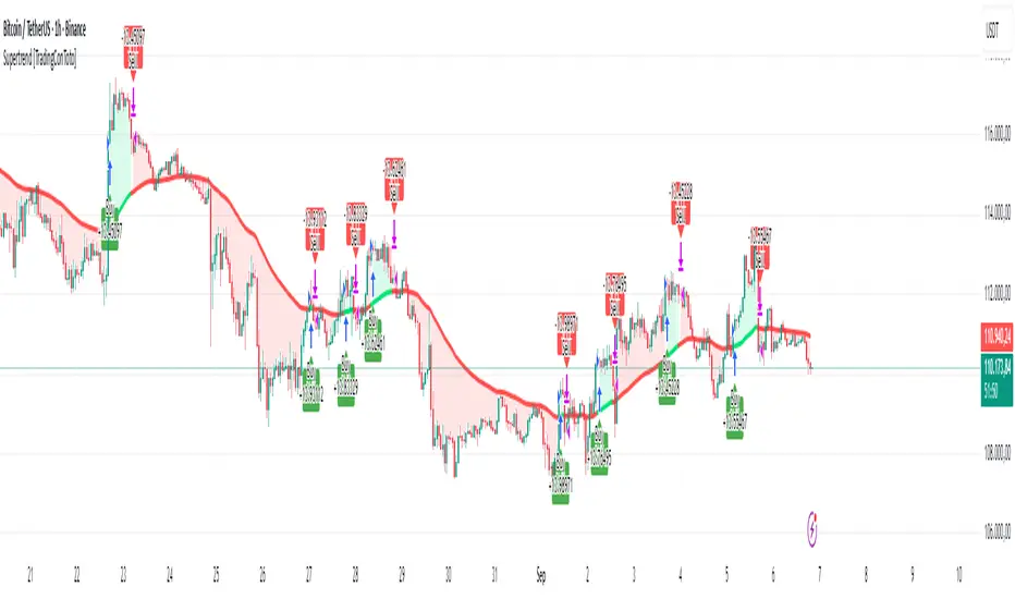
Supertrend [TradingConToto]Supertrend — ADX/DI + EMA Gap + Breakout (with Mobile UI)
What makes it original
Supertrend combines trend strength (ADX/DI), multi-timeframe bias (EMA63 and EMA 200D equivalent), a structural filter based on the distance between EMA2400 and EMA4800 expressed in ATR units, and a momentum confirmation through a previous high breakout.
This is not a random mashup — it’s a sequence of filters designed to reduce trades in ranging markets and prioritize mature trends:
Direction: +DI > -DI (trend led by buyers).
Strength: ADX > mean(ADX) (avoids weak, choppy phases).
Short-term bias: Close > EMA63.
Long-term bias: Close > EMA4800 ≈ EMA200 daily on H1.
Momentum: Close > High (immediate breakout).
Structure: (EMA2400 − EMA4800) > k·ATR (ensures separation in ATR units, filters out flat phases).
Entries & exits
Entry: when all six conditions are met and no open position exists.
Exit: if +DI < -DI or Close < EMA63.
Visuals: EMA63 is painted green while in position and red otherwise, with a supertrend-style band; “BUY” labels appear below the green band and “SELL” labels above the red band.
UI: includes a compact table (mobile-friendly) showing the state of each condition.
Default parameters used in this publication
Initial capital: 10,000
Position size: 10% of equity (≤10% per trade is considered sustainable).
Commission: 0.01% per side (adjust to your broker/market).
Slippage: 1 tick
Pyramiding: 0 (only one position at a time)
Adjust commission/slippage to match your market. For US equities, commissions are often per share; for spot crypto, 0.10–0.20% total is common. I publish with 0.01% per side as a conservative example to avoid overestimating results.
Recommended backtest dataset
Timeframe: H1
Multi-cycle window (e.g. 2015–today)
Symbols with high liquidity (e.g. NASDAQ-100 large caps, or BTC/ETH spot) to generate 100+ trades. Avoid cherry-picked short windows.
Why each filter matters
+DI > -DI + ADX > mean: reduce counter-trend trades and weak signals.
Close > EMA63 + Close > EMA4800: enforce trend alignment in short and long horizons.
Breakout High : requires immediate momentum, avoids early entries.
EMA gap in ATR units: blocks flat or compressed structures where EMA200D aligns with price.
Limitations
The breakout filter may skip healthy pullbacks; the design prioritizes continuation over perfect entry price.
No fixed trailing stop/TP; exits depend on trend degradation via DI/EMA63.
Results vary with real costs (commissions, slippage, funding). Adjust defaults to your broker.
How to use
Apply it on a clean chart (no other indicators when publishing).
Keep in mind the default parameters above; if you change them, mention it in your notes and use the same values in the Strategy Tester.
Ensure your dataset produces 100+ trades for statistical validity.
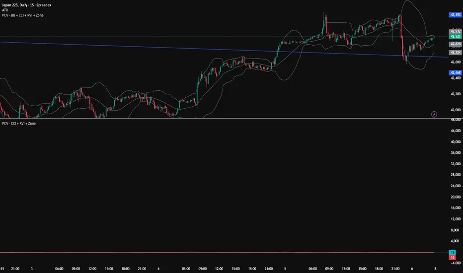
PCV (Darren.L-V2)Description:
This indicator combines Bollinger Bands, CCI, and RVI to help identify high-probability zones on M15 charts.
Features:
Bollinger Bands (BB) – displayed on the main chart in light gray. Helps visualize overbought and oversold price levels.
CCI ±100 levels + RVI – displayed in a separate sub-window:
CCI only shows the ±100 reference lines.
RVI displays a cyan main line and a red signal line.
Valid Zone Detection:
Candle closes outside the Bollinger Bands.
RVI crosses above +100 or below -100 (CCI level reference).
Candle closes back inside the BB, confirming a price rebound.
Requires two touches in the same direction to confirm the zone.
Only zones within 20–30 pips range are considered valid.
Usage:
Helps traders spot reversal or bounce zones with clear visual signals.
Suitable for all indices, Forex, and crypto on M15 timeframe.
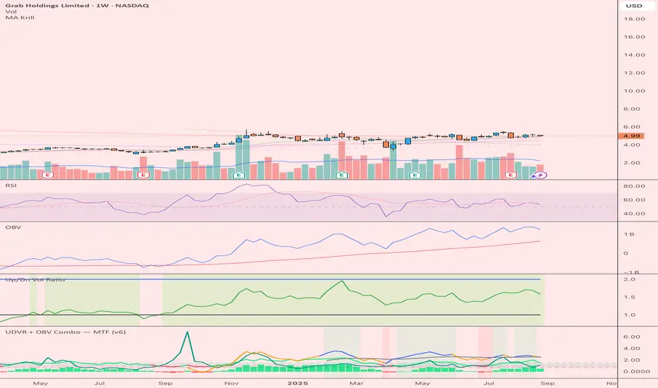
UDVR + OBV Combo — MTF (v6)The UDVR + OBV Combo is a multi-timeframe volume analysis tool that blends the Up/Down Volume Ratio with a normalized On-Balance Volume signal. It highlights when accumulation or distribution truly supports price action, adds higher-timeframe context, and shades the background when both indicators align. Use it to confirm breakouts, spot divergences, and filter trades with the backing of real volume flows.
1.Up/Down Volume Ratio (UDVR)
•Compares the rolling sum of up-volume (bars where price closed higher) vs down-volume (bars where price closed lower).
•A ratio > 1.0 = more accumulation (bullish pressure).
•A ratio < 1.0 = more distribution (bearish pressure).
•Optional histogram shows deviations from the 1.0 baseline.
•Customizable handling of equal closes (count as up, down, split, or ignore).
•Configurable lookback length and optional EMA smoothing.
2. On-Balance Volume (OBV)
•Classic cumulative OBV implemented natively (adds volume on up-bars, subtracts on down-bars).
•Normalized with a z-score so it can be compared across different symbols/timeframes.
•Includes an EMA signal line for slope detection.
•Alignment of OBV vs its EMA highlights rising or waning participation.
3. Multi-Timeframe Support
•Both UDVR and OBV can be plotted from a higher timeframe (HTF) (e.g. Daily UDVR shown on a 1h chart).
•Lets you see big-money accumulation/distribution while trading intraday.
•Shaded background when current TF and HTF agree (both bullish or both bearish).
How to read it
• Bullish confirmation = UDVR > 1 (accumulation) and OBV above EMA (rising participation).
• Bearish confirmation = UDVR < 1 (distribution) and OBV below EMA (falling participation).
• Mixed signals (e.g. UDVR > 1 but OBV falling) = caution; price may lack conviction.
• Divergences : If price makes a new high but OBV or UDVR does not, it’s a warning of weakening trend.
• Higher timeframe context : set HTF = Daily or Weekly and watch how short-term signals align with institutional flows. A long trade on the 15m chart is stronger when Daily UDVR is also above 1.
Inputs
•UDVR Lookback: number of bars for rolling volume sums.
•Smoothing EMA: smooths UDVR for stability.
•Equal Close Handling: decide how equal closes affect UDVR.
•Signal Band: optional UDVR extreme thresholds.
•Show Histogram: toggle UDVR histogram around baseline.
•Higher Timeframe UDVR: overlay Daily/Weekly UDVR on lower timeframe charts.
•OBV EMA length: slope proxy for normalized OBV.
•OBV Normalization window: controls z-score sensitivity.
•Higher Timeframe OBV: overlay higher timeframe OBV.
Alerts
•UDVR Bullish/Bearish cross at the 1.0 baseline.
•OBV slope up/down when OBV crosses its EMA.
•Alignment signals when UDVR and OBV agree (both confirm bullish or bearish conditions).
Why it’s useful
•Combines trend, momentum, and participation in one place.
•Helps avoid false breakouts by checking if volume supports the move.
•Lets you spot accumulation/distribution shifts before they show up in price.
•Gives a higher timeframe context so you’re not trading against the “big picture.”
Once applied, the indicator creates a dedicated pane below price with the following components:
UDVR Line (green/red)
• Green when UDVR > 1.0 (more up-volume than down-volume → accumulation).
• Red when UDVR < 1.0 (more down-volume → distribution).
UDVR Baseline and Bands
• Grey baseline at 1.0 = balance between buying and selling volume.
• Optional upper/lower bands (default 1.5 and 0.67) highlight extreme imbalances.
• Shaded areas between baseline and bands provide visual context for strength/weakness.
UDVR Histogram (optional)
• Columns around the baseline showing (UDVR – 1.0).
• Quick way to gauge how far above/below balance the ratio is.
Higher-Timeframe UDVR (teal line)
• Overlays the UDVR from a higher timeframe (e.g. Daily) on your intraday chart.
• Lets you see whether institutional flows support your shorter-term signals.
OBV Normalized (blue/orange line)
• Classic OBV, but normalized with a z-score so it stays readable across assets.
• Blue when OBV is above its EMA (rising participation).
• Orange when below its EMA (waning participation).
OBV EMA (grey line)
• Signal line showing the slope of OBV.
• Crosses between OBV and this line mark shifts in participation.
Higher-Timeframe OBV (purple line, optional)
• Plots OBV from a higher timeframe for additional context.
Background Shading
• Light green = both UDVR > 1 and OBV > OBV-EMA (bullish alignment).
• Light red = both UDVR < 1 and OBV < OBV-EMA (bearish alignment).
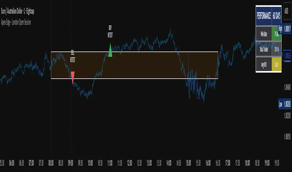
Apex Edge - London Open Session# Apex Edge - London Open Session Trading System
## Overview
The London Open Session indicator captures institutional price action during the first hour of the London forex session (8:00-9:00 AM GMT) and identifies high-probability breakout and retest opportunities. This system tracks the session's high/low range and generates precise entry signals when price breaks or retests these key institutional levels.
## Core Strategy
**Session Tracking**: Automatically identifies and marks the London Open session boundaries, creating a trading zone from the first hour's price range.
**Dual Entry Logic**:
- **Breakout Entries**: Triggers when price closes beyond the session high/low and continues in that direction
- **Retest Entries**: Activates when price returns to test the broken level as new support/resistance
**Performance Analytics**: Built-in win rate tracking displays real-time performance statistics over user-defined lookback periods, enabling data-driven optimization for each currency pair.
## Key Features
### Automated Zone Detection
- Precise London session timing with timezone offset controls
- Visual session boundaries with customizable colours
- Automatic high/low range calculation and display
### Smart Entry System
- Breakout confirmation requiring candle close beyond zone
- Retest detection with configurable pip distance tolerance
- Separate risk/reward ratios for breakout vs retest entries
- Visual entry arrows with clear trade direction labels
### Performance HUD
- Real-time win rate calculation over customizable periods (7-365 days)
- Total trades tracking with win/loss breakdown
- Average risk-reward ratio display
- Color-coded performance metrics (green >70%, yellow >50%, red <50%)
### PineConnector Integration
- Direct MT4/MT5 execution via PineConnector alerts
- Proper forex pip calculations for all currency pairs
- Customizable risk percentage per trade
- Symbol override capability for broker compatibility
- Automatic SL/TP level calculation in pips
## Critical Usage Requirements
### Pair-Specific Optimization
Each currency pair requires individual optimization due to varying volatility characteristics, institutional participation levels, and typical price ranges during London hours. The performance HUD is essential for identifying optimal settings before live trading.
**Recommended Testing Process**:
1. Apply indicator to desired currency pair and timeframe
2. Experiment with session timing - while 8:00-9:00 AM GMT is standard, some pairs may show improved performance with alternative hourly windows (e.g., 7:00-8:00 AM or 9:00-10:00 AM)
3. Adjust Stop Loss distances, Risk/Reward ratios, and Retest distances
4. Monitor win rate over 30+ day periods using the performance HUD
5. Only proceed with live alerts once consistent 60%+ win rates are achieved
6. Create separate optimized chart setups for each profitable pair/timeframe combination
### Timeframe Specifications
This indicator is specifically designed and tested for:
- **1-minute charts**: Optimal for capturing immediate institutional reactions
- **5-minute charts**: Balanced approach between noise reduction and opportunity frequency
Higher timeframes generally produce inferior results due to increased noise and reduced institutional edge during the London session window.
## Settings Configuration
### Session Timing
- **London Open/Close Hours**: Adjust for your chart's timezone
- **Rectangle End Time**: Set to 4:30 PM to stop signals before NY session close
- **Timezone Offset**: Ensure accurate London session capture
### Entry Parameters
- **Retest Distance**: 3-8 pips depending on pair volatility
- **Stop Loss Pips**: Separate settings for breakouts (10-15 pips) and retests (8-12 pips)
- **Risk/Reward Ratios**: Independent ratios for different entry types
### PineConnector Setup
- **License ID**: Your PineConnector license key
- **Symbol Override**: MT4/MT5 symbol names if different from TradingView
- **Risk Percentage**: Position size as percentage of account balance
- **Prefix/Comment**: Organize trades in terminal
## Manual Trading Limitations
Without PineConnector automation, traders face significant practical challenges:
**Settings Management**: Each currency pair requires different optimized parameters. Switching between charts means manually adjusting multiple settings each time, creating potential for errors and missed opportunities.
**Timing Sensitivity**: London Open signals can occur rapidly during high-volatility periods. Manual execution may result in slippage or missed entries.
**Multi-Pair Monitoring**: Tracking 4-11 currency pairs simultaneously while manually adjusting settings for each switch becomes impractical for most traders.
**Parameter Consistency**: Risk of using suboptimal settings when quickly switching between pairs, potentially compromising the careful optimization work.
## Recommended Workflow
1. **Historical Testing**: Use win rate HUD to identify profitable pairs and optimal parameters
2. **Demo Automation**: Test PineConnector alerts on demo accounts with optimized settings
3. **Live Implementation**: Deploy alerts only on proven profitable pair/timeframe combinations
4. **Ongoing Monitoring**: Regular review of performance metrics to maintain edge
## Risk Disclaimer
This indicator provides analysis tools and automation capabilities but does not guarantee profitable trading outcomes. Past performance does not predict future results. Users should thoroughly backtest and demo trade before risking live capital. The London session strategy works best during specific market conditions and may underperform during low volatility or unusual market environments.
## Support Requirements
Successful implementation requires:
- Basic understanding of London session market dynamics
- PineConnector subscription for automation features
- Patience for proper optimization process
- Realistic expectations about win rates and drawdown periods
This system is designed for serious traders willing to invest time in proper optimization and risk management rather than plug-and-play solutions.
Alt Season vs USDT Flow DashboardWhat the script tells you (the signals)
It builds four “alt vs stables” lenses and colors the background when they agree.
ALT ex-ETH / STABLES (TOTAL3 / (USDT+USDC+DAI))
Think: “How much alt cap per $1 of dry-powder stables?”
Bullish when price is above its 200-day SMA and rising → risk appetite expanding toward smaller alts.
ALT Share of Risk-On ((TOTAL − STABLES − BTC − ETH) / (TOTAL − STABLES))
Of the non-stable crypto pie, how much is flowing to ex-BTC/ETH alts?
Uptrend = broadening alt participation (late-early to mid alt-season behavior).
Dominance Spread ((TOTAL3 / TOTAL) − (STABLES / TOTAL))
Alts’ share minus stables’ share.
Widening spread means stables are being converted into alts (not just into BTC).
Flow Ratio ROC(TOTAL3, N) / ROC(STABLES, N) (default N=30 days)
Compares alts’ growth rate to stable supply growth.
> 1 and sustained → alts expanding faster than new “dry powder” is appearing.
The background color (“regime”)
Green (ALT-on) when all three conditions align:
ALT/Stable > its SMA
Dominance Spread > its SMA
Flow Ratio > 1
Red (ALT-off) when the opposite holds.
No color = mixed/chop.
How to read it (quick playbook)
Early alt-season tell:
BTC.D starts to slip, total market cap (TOTAL) rising.
ALT/Stable breaks above its 200-SMA and stays there.
Dominance Spread climbs (alts gaining share, stables losing share).
Flow Ratio > 1 for a few weeks.
Maturing phase: ALT Share of Risk-On rises (money broadens from ETH/L1s → mid/small caps).
Exhaustion/false start: Flow Ratio dips < 1 or ALT/Stable loses the 200-SMA while BTC.D stabilizes or rises.
Practical tips
Timeframes: Make calls on 1D. Use 1W to avoid whipsaw; use 4H only for entries once the 1D regime is green.
Smoothing: If you see noisy spikes from market-cap revisions, add a light smoother (e.g., 7D SMA on the plotted lines).
Parameters:
Try ROC length 21–45 days.
Try SMA 150–250 days (200 is a good middle).
Confluence: Keep BTC.D and ETH.D in another pane. Best alt windows: BTC.D trending down, ETH.D flat-to-up initially, then ETH.D flattens as TOTAL3 momentum spreads to mid/small caps.
Risk checks: If USDT.D/USDC.D (stable dominance) spike up while your signals are green, that’s a caution flag (capital retreating to stables).

Scalping Line Strategy📌 Scalping Line Strategy – A Precision Crossover System
🔎 Overview
The Scalping Line Strategy is a short-term trading system built around the concept of momentum-driven crossovers between a smoothed moving average filter and a fast signal line. It is designed for scalpers and intraday traders who seek clear entry signals, minimal lag, and adaptive filtering to fit volatile market conditions.
At its core, the strategy uses a custom signal line ("Scalping Line"), which is derived from the difference between a double-smoothed moving average and a shorter-period signal line. Trade entries are triggered when this Scalping Line crosses above or below zero, providing a clean and rules-based framework for both long and short setups.
⚙️ Core Logic
Main Trend Filter – A double-smoothed moving average is calculated over a configurable period (default 100). This reduces noise and provides a more robust backbone for scalping signals.
Percent-Based Filter – To avoid false signals, a customizable percentage filter adjusts how closely the system “respects” price deviations from the moving average. This helps filter out insignificant fluctuations.
Signal Line – A shorter-period simple moving average (default 7) provides faster responsiveness to recent price action.
Scalping Line (SLI) – Calculated as the difference between the fast signal line and the smoothed moving average. When the SLI crosses zero, it signals a potential momentum shift.
SLI > 0 → Momentum bias is bullish.
SLI < 0 → Momentum bias is bearish.
🎯 Trade Direction & Flexibility
Trade Direction Control:
Choose between Long Only, Short Only, or Both to tailor the system to your trading style.
Signal Flip Option:
By default, long entries occur when the SLI crosses below zero, and shorts when it crosses above zero. This orientation can be flipped, allowing for alternative interpretations of the signals depending on how you want to capture momentum in your market.
🕒 Time Window Filtering
For intraday traders, a time filter can be enabled to restrict signals to specific trading sessions (e.g., 9 AM – 4 PM EST). This is particularly useful when trading assets such as equities or futures that have strong intraday volatility windows.
📈 Visuals & Clarity
Scalping Line Plot: Displayed as a dynamic oscillator around a zero baseline.
Histogram Fill: Green when above zero (bullish bias), red when below zero (bearish bias).
Signal Markers: Clear arrows mark long and short entries at crossover points.
Zero Line Reference: A flat gray line at zero assists in visually gauging momentum shifts.
🚀 Strategy Execution
Long Entry: Triggered when SLI crosses below zero (or above zero if flip is enabled) within allowed session hours.
Short Entry: Triggered when SLI crosses above zero (or below zero if flip is enabled) within allowed session hours.
Built-in Signal Cancels: Pending entries are canceled if conditions are no longer valid, ensuring no stale trades remain active.
✅ Best Use Cases
Markets: Works across equities, forex, crypto, and futures with sufficient intraday volatility.
Timeframes: Most effective on 1m to 15m charts for scalping setups, but adaptable to higher frames for swing trading.
Style: Traders who appreciate simple, rules-based momentum crossovers will find this system easy to follow and highly adaptable.
⚠️ Risk Management Note
This strategy is strictly an entry signal framework. Position sizing, stop-loss, and take-profit rules must be overlaid based on your risk management style. Always validate results with backtesting and forward testing before applying to live trading accounts.
📜 Final Thoughts
The Scalping Line Strategy offers a refined, easy-to-interpret approach to intraday trading. By combining smoothed moving averages, adaptive filtering, and flexible signal options, it helps traders identify short-term momentum shifts with clarity and confidence, making it a highly configurable tool for scalping-focused strategies.

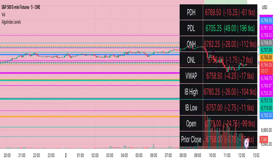
RTH Levels: VWAP + PDH/PDL + ONH/ONL + IBAlgo Index — Levels Pro (ONH/ONL • PDH/PDL • VWAP±Bands • IB • Gaps)
Purpose. A session-aware, non-repainting levels tool for intraday decision-making. Designed for futures and indices, with clean visuals, alerts, and a one-click Minimal Mode for screenshot-ready charts.
What it plots
• PDH/PDL (RTH-only) – Prior Regular Trading Hours high/low, computed intraday and frozen at the RTH close (no 24h mix-ups, no repainting).
• ONH/ONL – Prior Overnight high/low, held throughout RTH.
• RTH VWAP with ±σ bands – Volume-weighted variance, reset each RTH.
• Initial Balance (IB) – First N minutes of RTH, plus 1.5× / 2.0× extensions after IB completes.
• Today’s RTH Open & Prior RTH Close – With gap detection and “gap filled” alert.
• Killzone shading – NY Open (09:30–10:30 ET) and Lunch (11:15–13:30 ET).
• Values panel (top-right) – Each level with live distance in points & ticks.
• Right-edge level tags – With anti-overlap (stagger + vertical jitter).
• Price-scale tags – Native trackprice markers that always “stick” to the axis.
⸻
New in v6.4
• Minimal Mode: one click for a clean look (thinner lines, VWAP bands/IB extensions hidden, on-chart right-edge labels off; price-scale tags remain).
• Theme presets: Dark Hi-Contrast / Light Minimal / Futures Classic / Muted Dark.
• Anti-overlap controls: horizontal staggering, vertical jitter, and baseline offset to keep tags readable even when levels cluster.
⸻
Quick start (2 minutes)
1. Add to chart → keep defaults.
2. Sessions (ET):
• RTH Session default: 09:30–16:00 (US equities cash hours).
• Overnight Session default: 18:00–09:29.
Adjust for your market if you use different “day” hours (e.g., many use 08:20–13:30 ET for COMEX Gold).
3. Theme & Minimal Mode: pick a Theme Preset; enable Minimal Mode for screenshots.
4. Visibility: toggle PD/ON/VWAP/IB/References/Panel to taste.
5. Right-edge labels: turn Show Right-Edge Labels on. If they crowd, tune:
• Anti-overlap: min separation (ticks)
• Horizontal offset per tag (bars)
• Vertical jitter per step (ticks)
• Right-edge baseline offset (bars)
6. Alerts: open Add alert → Condition: and pick the events you want.
⸻
How levels are computed (no repainting)
• PDH/PDL: Intraday H/L are accumulated only while in RTH and saved at RTH close for “yesterday’s” values.
• ONH/ONL: Accumulated across the defined Overnight window and then held during RTH.
• RTH VWAP & ±σ: Volume-weighted mean and standard deviation, reset at the RTH open.
• IB: First N minutes of RTH (default 60). Extensions (1.5×/2.0×) appear after IB completes.
• Gaps: Today’s RTH open vs prior RTH close; “Gap Filled” triggers when price trades back to prior close.
⸻
Practical playbooks (how to trade around the levels)
1) PDH/PDL interactions
• Rejection: Price taps PDH/PDL then closes back inside → mean-reversion toward VWAP/IB.
• Acceptance: Close/hold beyond PDH/PDL with momentum → continuation to next HTF/IB target.
• Alert: PD Touch/Break.
2) ONH/ONL “taken”
• Often one ON extreme is taken during RTH. ONH Taken / ONL Taken → check if it’s a clean break or sweep & reclaim.
• Sweep + reclaim near VWAP can fuel rotations through the ON range.
3) VWAP ±σ framework
• Balanced: First tag of ±1σ often reverts toward VWAP.
• Trend: Persistent trade beyond ±1σ + IB break → target ±2σ/±3σ.
• Alerts: VWAP Cross and VWAP Reject (cross then immediate fail back).
4) IB breaks
• After IB completes, a clean IB break commonly targets 1.5× and sometimes 2.0×.
• Quick return inside IB = possible fade back to the opposite IB edge/VWAP.
• Alerts: IB Break Up / Down.
5) Gaps
• Gap-and-go: Opening drive away from prior close + VWAP support → trend until IB completion.
• Gap-fill: Weak open and VWAP overhead/underfoot → trade toward prior close; manage on Gap Filled alert.
Pro tip: Stack confluences (e.g., ONL sweep + VWAP reclaim + IB hold) and respect your execution rules (e.g., require a 5-minute close in direction, or your order-flow confirmation).
⸻
Inputs you’ll actually touch
• Sessions (ET): Session Timezone, RTH Session, Overnight Session.
• Visibility: toggles for PD/ON/VWAP/IB/Ref/Panel.
• VWAP bands: set σ multipliers (±1/±2/±3).
• IB: duration (minutes) and extension multipliers (1.5× / 2.0×).
• Style & Theme: Theme Preset, Main Line Width, Trackprice, Minimal Mode, and anti-overlap controls.
⸻
Alerts included
• PD Touch/Break — High ≥ PDH or Low ≤ PDL
• ONH Taken / ONL Taken — First in-RTH take of ONH/ONL
• VWAP Cross — Close crosses VWAP
• VWAP Reject — Cross then immediate fail back
• IB Break Up / Down — Break of IB High/Low after IB completes
• Gap Filled — Price trades back to prior RTH close
Setup: Add alert → Condition: Algo Index — Levels Pro → choose event → message → Notify on app/email.
⸻
Panel guide
The top-right panel shows each level plus live distance from last price:
LevelValue (Δpoints | Δticks)
Coloring: green if level is below current price, red if above.
⸻
Styling & screenshot tips
• Use Theme Preset that matches your chart.
• For dark charts, “Dark Hi-Contrast” with Main Line Width = 3 works well.
• Enable Trackprice for crisp axis tags that always stick to the right edge.
• Turn on Minimal Mode for cleaner screenshots (no VWAP bands or IB extensions, on-chart tags off; price-scale tags remain).
• If tags crowd, increase min separation (ticks) to 30–60 and horizontal offset to 3–5; add vertical jitter (4–12 ticks) and/or push tags farther right with baseline offset (bars).
⸻
Behavior & limitations
• Levels are computed incrementally; tables refresh on the last bar for efficiency.
• Right-edge labels are placed at bar_index + offset and do not track extra right-margin scrolling (TradingView limitation). The price-scale tags (from trackprice) do track the axis.
• “RTH” is what you define in inputs. If your market uses different day hours, change the session strings so PDH/PDL reflect your definition of “yesterday’s session.”
⸻
FAQ
Q: My PDH/PDL don’t match the daily chart.
A: By design this uses RTH-only highs/lows, not 24h daily bars. Adjust sessions if you want a different definition.
Q: Right-edge tags overlap or don’t sit at the far right.
A: Increase min separation / horizontal offset / vertical jitter and/or push tags farther with baseline offset. If you want markers that always hug the axis, rely on Trackprice.
Q: Can I change killzones?
A: Yes—edit the session strings in settings or request a version with user inputs for custom windows.
⸻
Disclaimer
Educational use only. This is not financial advice. Always apply your own risk management and confirmation rules.
⸻
Enjoy it? Please ⭐ the script and share screenshots using Minimal Mode + a Theme Preset that fits your style.
VWAP Suite {Phanchai}VWAP Suite {Phanchai}
Compact, readable, TradingView-friendly.
What is VWAP?
The Volume Weighted Average Price (VWAP) is the average price of a period weighted by traded volume. It’s used as a fair-value reference (mean) and resets at the start of each new period.
Included VWAP Modes
Session — resets each trading day (current session).
Week / Month / Quarter / Year — current calendar periods.
Anchored Week / Month / Quarter / Year — starts at the beginning of the previous completed period.
Rolling 7D / 30D / 90D — rolling windows: today + last 6/29/89 daily sessions.
Important
This suite does not generate buy/sell signals. It provides structure and confluence; decisions remain yours.
Use Cases
Identify fair-value zones / mean-reversion areas.
Plan TP / SL around periodic VWAPs.
Define DCA levels (e.g., anchored to prior week/month).
Gauge trend bias via VWAP slope and reactions.
How to Use
Inputs → VWAP 1..5: Choose the period per slot (Session, Anchored, Rolling, etc.) and toggle Show .
Sources: Select the price source for all VWAPs (default: HLC3).
Global: Line offset (bars) shifts plots visually (does not affect calculations).
Style tab: Adjust per-line colors, thickness, and line style.
Alerts
Price crosses a VWAP (per slot).
VWAP slope turns UP or DOWN (per slot).
Tips & Notes
Volume required: Poor/absent volume (e.g., some FX tickers) can degrade accuracy.
Anchored modes: Start at the prior period’s open; values appear only after that timestamp.
Rolling modes: Use completed daily sessions (including today).
Clutter control: If labels crowd, increase Line offset or hide unneeded slots.
Confluence: Combine with market structure, liquidity zones, or momentum filters for stronger context.
Built for clear VWAP workflows. Trade safe!

Market Open Impulse [LuciTech]Market Open Impulse Strategy
The Market Open Impulse Strategy is designed to capture significant price movements that occur at market open (2:30 PM UK time). This strategy identifies impulsive candles with high volatility and enters trades based on the direction and strength of the initial market reaction.
How It Works:
The strategy activates exclusively at 2:30 PM UK time during market open sessions. It uses ATR-based volatility filtering to identify impulsive candles that exceed a configurable multiplier (default 1.5x ATR). Long entries are triggered when an impulsive candle closes above its midpoint and above the opening price, while short entries occur when an impulsive candle closes below its midpoint and below the opening price.
Risk management is handled through precise stop loss placement at the opposite extreme of the impulse candle (high for short positions, low for long positions). Take profit levels are calculated using a configurable risk-reward ratio with a default setting of 3:1. Position sizing is automatically calculated based on the percentage risk per trade, and an optional breakeven feature can move the stop loss to the entry price at specified profit levels.
The strategy incorporates time-based filtering to ensure trades only occur during the specified market open window. Visual indicators highlight qualifying impulsive candles and plot all entry and exit levels for clear trade management. The system offers flexible risk management with customizable risk percentage, risk-reward ratios, and breakeven settings, along with multiple stop loss calculation methods including both ATR-based and candle-based options.
Key Parameters:
Market open timing is fully configurable through hour and minute settings for strategy activation. The impulse ATR multiple sets the minimum volatility threshold required for trade qualification, with visual highlighting available for qualifying setups. Risk management parameters include the percentage of account equity to risk per trade, target profit multiples relative to initial risk, and the profit level threshold for breakeven stop loss adjustment. Users can choose between ATR-based or candle-based stop loss calculation methods and adjust technical parameters for volatility calculation including ATR length and smoothing methods.
Applications:
This strategy is particularly effective for trading market open volatility and momentum, capturing institutional order flow during key timing windows, executing short-term swing trades on significant price impulses, and trading markets with predictable opening patterns and consistent volatility characteristics.

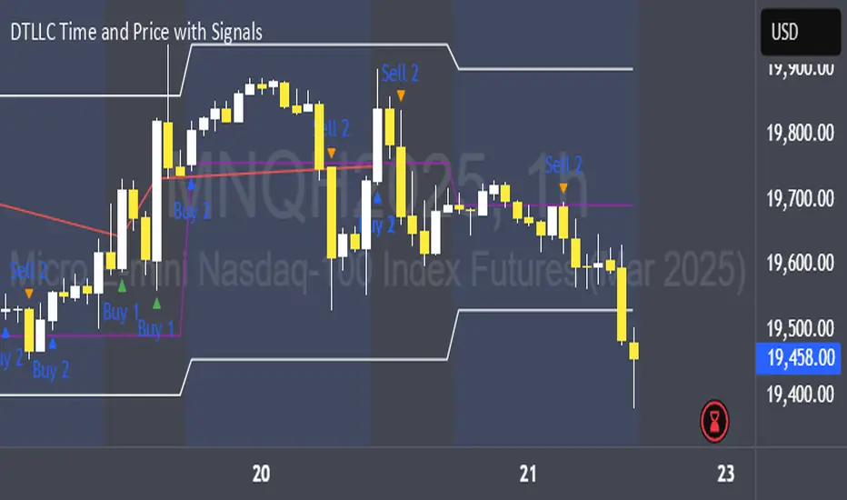
DTLLC Time & PriceDTLLC Time and Price with Signals
This indicator is built for traders who understand ICT concepts and want a structured, visual way to align time-based price action with key market levels. By combining customizable trading windows, breakout logic, and daily reference points, it helps you identify high-probability trade opportunities while filtering out market noise.
Key Features
1. Dual Custom Time Ranges (Kill Zones)
Set two independent time ranges per day (start/end hour and minute).
Each range identifies the highest high and lowest low within its window.
Built-in breakout detection generates buy/sell signals when price moves beyond these levels.
2. Volatility Filtering
Adjustable volatility threshold based on True Range relative to ATR.
Filters out low-quality signals during choppy, low-volatility conditions.
3. ATR-Based Stop Loss
Custom ATR length and stop-loss multiplier settings.
Automatically plots ATR-based stop levels for triggered trades.
4. Daily Key Levels
Plots Previous Day High, Previous Day Low, and Midnight Open continuously on the chart.
Useful for spotting breakout and reversal opportunities in line with ICT market structure concepts.
5. Liquidity & Engulfing Candle Highlights
Highlights potential liquidity grab zones (yellow candles) when significant highs/lows are set within your lookback period.
Detects bullish (green) and bearish (red) engulfing patterns for added confluence.
6. Visual & Signal Tools
Buy/Sell signals plotted directly on chart (separate colors for Range 1 and Range 2). Continuous plotting of reference levels to maintain market context throughout the session.
Example Use Case:
A common ICT-inspired reversal setup:
Wait for price to sweep the Previous Day’s High or Low during your chosen time range.
Look for a buy or sell signal with volatility confirmation.
Manage risk using the ATR-based stop-loss plot.
Disclaimer: This script is for educational purposes only and is not financial advice. Trade responsibly and always test strategies before applying them in live markets.
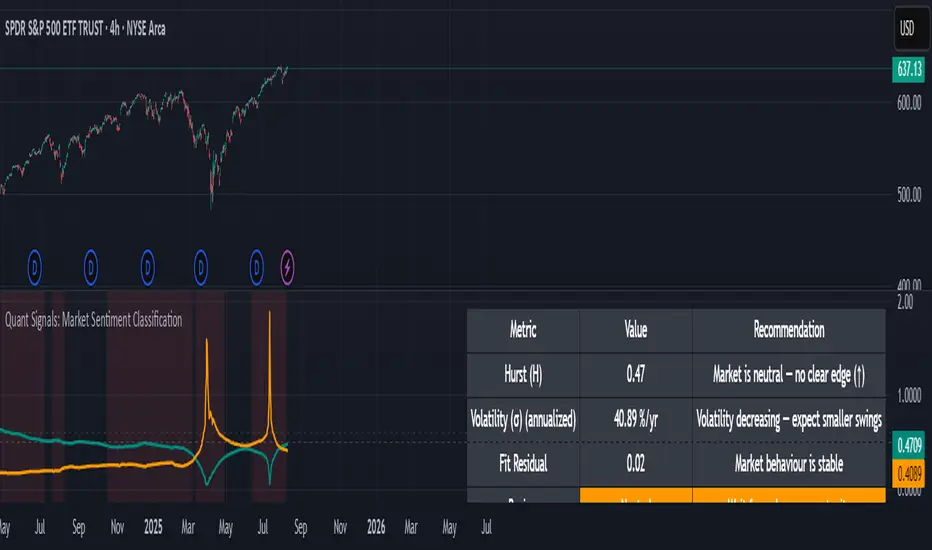
Quant Signals: Market Sentiment Monitor HUDWavelets & Scale Spectrum
This indicator is ideal for traders who adapt their strategy to market conditions — such as swing traders, intraday traders, and system developers.
Trend-followers can use it to confirm trending conditions before entering.
Mean-reversion traders can spot choppy markets where reversals are more likely.
Risk managers can monitor volatility shifts and regime changes to adjust position size or pause trading.
It works best as a market context filter — telling you the “weather” before you decide on the trade.
Wavelets are like tiny “measuring rulers” for price changes. Instead of looking at the whole chart at once, a wavelet looks at differences in price over a specific time scale — for example, 2 bars, 4 bars, 8 bars, and so on.
The scale spectrum is what you get when you measure volatility at several of these scales and then plot them against scale size.
If the spectrum forms a straight line on a log–log chart, it means price changes follow a consistent pattern across time scales (a power-law relationship).
The slope of that line gives the Hurst exponent (H) — telling you whether moves tend to persist (trend) or reverse (mean-revert).
The height of the line gives you the volatility (σ) — the average size of moves.
This approach works like a microscope, revealing whether the market’s behaviour is consistent across short-term and long-term horizons, and when that behaviour changes.
This tool applies a wavelet-based scale-spectrum analysis to price data to estimate three key market state measures inside a rolling window:
Hurst exponent (H) — measures persistence in price moves:
H > ~0.55 → market is trending (moves tend to continue).
H < ~0.45 → market is choppy/mean-reverting (moves tend to reverse).
Values near 0.5 indicate a neutral, random-walk-like regime.
Volatility (σ) — the average size of price swings at your chart’s timeframe, optionally annualized. Rising volatility means larger price moves, falling volatility means smaller moves.
Fit residual — how well the observed multi-scale volatility fits a clean power-law line. Low residual = stable behaviour; high residual = structural change (possible regime shift).
AI Breakout Bands (Zeiierman)█ Overview
AI Breakout Bands (Zeiierman) is an adaptive trend and breakout detection system that combines Kalman filtering with advanced K-Nearest Neighbor (KNN) smoothing. The result is a smart, self-adjusting band structure that adapts to dynamic market behavior, identifying breakout conditions with precision and visual clarity.
At its core, this indicator estimates price behavior using a two-dimensional Kalman filter (position + velocity), then enhances the smoothing process with a nonlinear, similarity-based KNN filter. This unique blend enables it to handle noisy markets and directional shifts with both speed and stability — providing breakout traders and trend followers a reliable framework to act on.
Whether you're identifying volatility expansions, capturing trend continuations, or spotting early breakout conditions, AI Breakout Bands gives you a mathematically grounded, visually adaptive roadmap of real-time market structure.
█ How It Works
⚪ Kalman Filter Engine
The Kalman filter models price movement as a state system with two components:
Position (price)
Velocity (trend direction)
It recursively updates predictions using real-time price as a noisy observation, balancing responsiveness with smoothness.
Process Noise (Position) controls sensitivity to sudden moves.
Process Noise (Velocity) controls smoothing of directional flow.
Measurement Noise (R) defines how much the filter "trusts" live price data.
This component alone creates a responsive yet stable estimate of the market’s center of gravity.
⚪ Advanced K-Neighbor Smoothing
After the Kalman estimate is computed, the script applies a custom K-Nearest Neighbor (KNN) smoother.
Rather than averaging raw values, this method:
Finds K most similar past Kalman values
Weighs them by similarity (inverse of absolute distance)
Produces a smoother that emphasizes structural similarity
This nonlinear approach gives the indicator an AI feature — reacting fast when needed, yet staying calm in consolidation.
█ How to Use
⚪ Trend Recognition
The line color shifts dynamically based on slope direction and breakout confirmation.
Bullish conditions: price above the mid band with positive slope
Bearish conditions: price below the mid band with negative slope
⚪ Breakout Signals
Price breaking above or below the bands may signal momentum acceleration.
Combine with your own volume or momentum confirmation for stronger entries.
Bands adapt to market noise, helping filter out low-quality whipsaws.
█ Settings
Process Noise (Position): Controls Kalman filter’s sensitivity to price changes.
Process Noise (Velocity): Controls smoothing of directional component.
Measurement Noise (R): Defines how much trust is placed in price data.
K-Neighbor Length: Number of historical Kalman values considered for smoothing.
Slope Calculation Window: Number of bars used to compute trend slope of the smoothed Kalman.
Band Lookback (MAE): Rolling period for average absolute error.
Band Multiplier: Multiplies MAE to determine band width.
-----------------
Disclaimer
The content provided in my scripts, indicators, ideas, algorithms, and systems is for educational and informational purposes only. It does not constitute financial advice, investment recommendations, or a solicitation to buy or sell any financial instruments. I will not accept liability for any loss or damage, including without limitation any loss of profit, which may arise directly or indirectly from the use of or reliance on such information.
All investments involve risk, and the past performance of a security, industry, sector, market, financial product, trading strategy, backtest, or individual's trading does not guarantee future results or returns. Investors are fully responsible for any investment decisions they make. Such decisions should be based solely on an evaluation of their financial circumstances, investment objectives, risk tolerance, and liquidity needs.

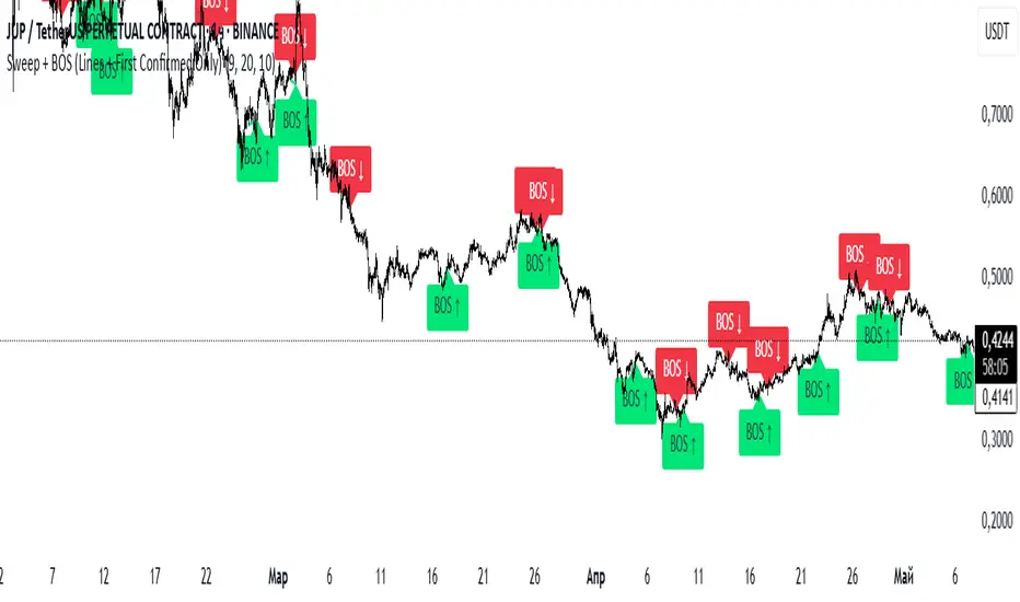
Sweep + BOS (Lines + First Confirmed Only)🔍 Indicator: Sweep + BOS (Break of Structure with Visual Lines)
🧠 Overview
This indicator combines Swing detection, Liquidity Sweeps, and Break of Structure (BOS) logic, with:
Customizable swing length,
BOS signals only after confirmed sweeps,
BOS shown only once per sweep,
Visual labels and connecting lines to highlight structure breaks clearly.
⚙️ Inputs
Swing Length:
Defines how many candles to use to identify a swing high/low. Must be an odd number (e.g., 3, 5, 7...).
Sweep Lookback Window:
Sets how far back the script checks for a sweep (false breakout over a swing).
BOS Validity After Sweep:
Number of bars within which a BOS can be considered valid after a sweep.
Toggle Options:
Show/hide:
Swing Labels
Sweep Labels
BOS Labels
BOS Connecting Lines
📌 Logic Breakdown
✅ Swings
Swing High: A candle’s high is greater than the highs of all N candles on both sides.
Swing Low: A candle’s low is lower than the lows of all N candles on both sides.
💧 Liquidity Sweeps
Sweep High:
Price spikes above a previous Swing High,
Then closes back below it (false breakout).
Sweep Low:
Price drops below a previous Swing Low,
Then closes back above it.
🔁 Break of Structure (BOS)
A BOS is only shown if:
It occurs after a valid sweep (within X bars),
It hasn’t been already plotted for that sweep,
BOS ↑ is only possible after Sweep Low,
BOS ↓ is only possible after Sweep High,
Opposite BOS type resets the last BOS state.
BOS ↑ (Bullish):
Confirmed when price closes above previous Swing High after Sweep Low.
Label appears at the candle low.
A line is drawn from the Swing Low to the BOS candle.
BOS ↓ (Bearish):
Confirmed when price closes below previous Swing Low after Sweep High.
Label appears at the candle high.
A line is drawn from the Swing High to the BOS candle.
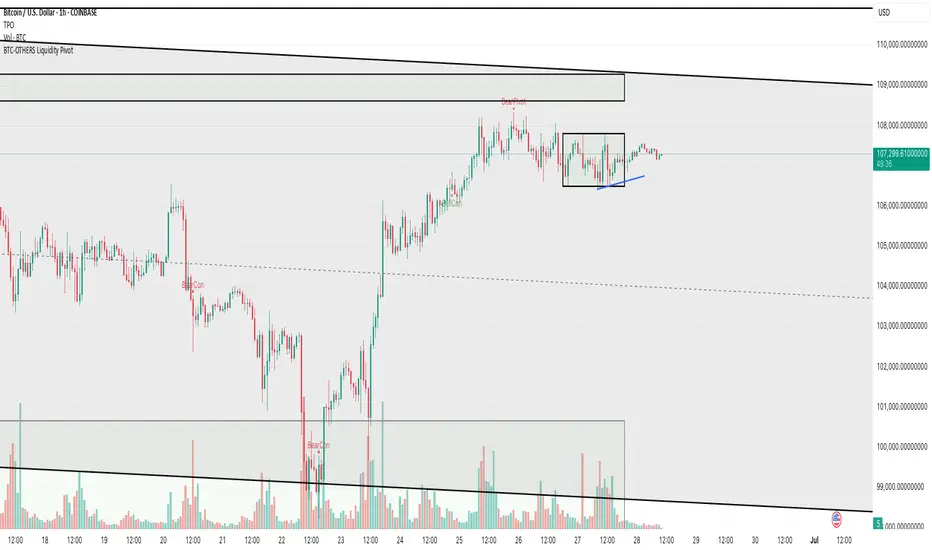
BTC-OTHERS Liquidity PivotBTC-OTHERS Liquidity Map – 1-hour Multi-Asset Pivot Scanner
WHAT IT DOES
This script tracks liquidity shifts between Bitcoin (BTC) and the broader alt-coin market (the OTHERS market-cap index that excludes the top-10 coins). It labels every confirmed 1-hour swing high or low on both assets, then flags four states:
BearPivot – BTC prints a new swing High while OTHERS does not; liquidity crowds into BTC and alts are weak.
BullPivot – BTC prints a swing Low and OTHERS forms a Higher Low; fresh liquidity starts flowing into stronger alts.
BearCon – BTC prints a swing Low and OTHERS forms a Lower Low; down-trend continuation.
BullCon – No new BTC Low while OTHERS makes a Higher High; up-trend continuation.
Signals appear on the actual pivot bar (offset back by the look-back length), so they never repaint after confirmation.
HOW THE PIVOTS ARE FOUND
• Symmetrical window: “Pivot Len” bars to the left and right (default 21).
• Full confirmation on both sides delivers stable, non-repainting pivots at the cost of about Pivot Len bars’ delay.
• Labels are offset –Pivot Len so they sit on the genuine extreme.
INPUTS
Symbols: BTC symbol and an OTHERS symbol so you can switch exchanges or choose another alt index.
Pivot Len: tighten for faster but noisier signals; widen for cleaner pivots.
Style: customise shape and text colours.
PLOTS AND ALERTS
Four labelled shapes (BearPivot, BullPivot, BearCon, BullCon) plot above or below price. Each label is linked to an alertcondition, so you can create one-click alerts and stay informed without watching the screen.
TYPICAL WORKFLOW
1. Attach the script to any 1-hour BTC chart (or leave the script’s timeframe empty to follow your current chart TF).
2. Turn on alerts to receive push/email notifications.
3. Use the labels as a liquidity compass, combining them with volume, funding or your own strategy for actual entries and exits.
Enjoy and trade safe.
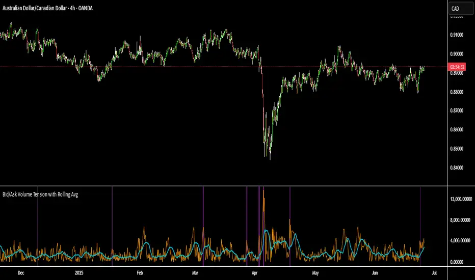
Bid/Ask Volume Tension with Rolling Avg📊 Bid/Ask Volume Tension with Rolling Average
This indicator is designed to help traders identify pivotal moments of buildup, exhaustion, or imbalance in the market by calculating the tension between buy and sell volume.
🔍 How It Works:
Buy volume is approximated when the candle closes higher than or equal to its open.
Sell volume is approximated when the candle closes below its open.
Both are smoothed using an EMA (Exponential Moving Average) for noise reduction.
Tension is calculated as the absolute difference between smoothed buy and sell volume.
A rolling average of tension shows the baseline for normal behavior.
When instant tension rises significantly above the rolling average, it often signals:
A build-up before a large move
Aggressive order flow imbalances
Potential reversals or breakouts
🧠 How to Use:
Watch the orange line (instant tension) for spikes above the aqua line (rolling average).
Purple background highlights show when tension exceeds a customizable multiple of the average — a potential setup zone.
Use this indicator alongside:
Price action (candlestick structure)
Support/resistance
Liquidity zones or order blocks
⚙️ Settings:
Smoothing Length: Controls the responsiveness of buy/sell volume smoothing.
Rolling Avg Window: Defines the lookback period for the baseline tension.
Buildup Threshold: Triggers highlight zones when tension exceeds this multiple of the average.
🧪 Best For:
Spotting pre-breakout tension
Detecting volume-based divergences
Confirming order flow imbalances
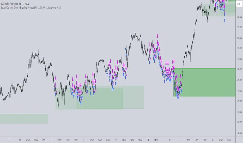
Supply/Demand Zones + Engulfment-based ExecutionSupply/Demand Zones + Engulfment-Based Execution
Strategy Overview
This strategy combines institutional trading concepts—supply/demand zones and engulfing candle patterns—to generate high-probability long and short trade setups. The system uses aggregated price action to identify potential reversal zones and confirms entries with engulfing candle patterns, ensuring trades are only taken when market structure shows commitment in the direction of the trade.
Core Concepts
• Supply & Demand Zones: These are automatically detected by analyzing aggregated bullish and bearish candle structures over user-defined intervals. Supply zones are formed after bearish continuation patterns; demand zones appear after bullish continuation patterns.
• Engulfing Entries: Once price enters a zone, the strategy waits for a bullish engulfing pattern (in a demand zone) or a bearish engulfing pattern (in a supply zone) before executing a trade. This adds confirmation and reduces false signals.
• Risk Management: Stop-loss is placed at the low (for long trades) or high (for short trades) of the engulfed candle. Take-profit can be calculated using a fixed R-multiple (risk-to-reward ratio) or a user-defined target price.
Key Features
Fully customizable aggregation factor for zone detection
Visual zone boxes, entry/SL/TP boxes, and engulfing pattern labels
Optional removal of mitigated zones for cleaner charting
Configurable trade mode (Long only, Short only, or Both)
Support for trading sessions and date filtering
Alerts for price entering supply or demand zones
How to Use
Select Aggregation Factor: Choose how many candles to group together for identifying key zones (e.g., 4x timeframe).
Enable Zones: Turn on supply and/or demand zones as needed.
Set Execution Parameters:
– Choose R-multiple (e.g., 2:1 risk-reward)
– Or use a fixed take-profit price
Define Trade Time Window:
– Set the date and time ranges to restrict execution
– Use Start Hour and End Hour to limit trades to specific sessions (e.g., London/New York)
Run on Desired Timeframe: Typically used on 15m–4H charts, depending on your strategy and the asset’s volatility.
Ideal For
• Traders using Smart Money Concepts (SMC)
• Those who value high-confluence entries
• Intraday to swing traders looking for structure-based automation
⚠️ Important Notes
• The strategy requires engulfing confirmation within the zone to enter a position.
• This script does not repaint and executes trades on a bar close basis.
• Backtest results may vary based on session filters and aggregation factor.
© Attribution
This strategy was developed by The_Forex_Steward and is licensed under the Mozilla Public License 2.0.
You are free to use, modify, and distribute it under the terms of that license.
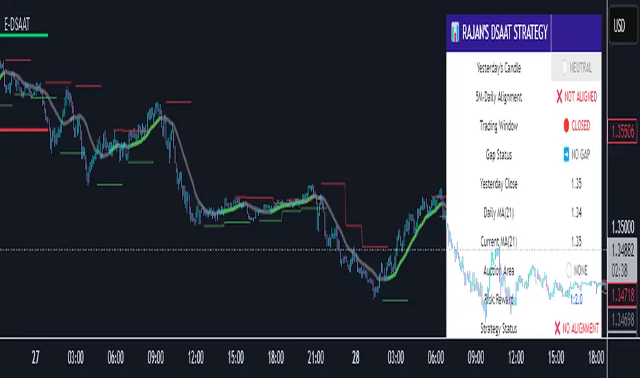
Enhanced Daily Sentiment & Auction Area Trading StrategyDetermine Daily Sentiment (Anchor Chart - Daily TF):
Analyze Yesterday's Daily Candle: Look at the previous day's daily candlestick (high, low, open, close). This is the "most important information."
Establish Bias: If yesterday's candle was bullish (closed higher), the bias for today is generally long (approx. 80% of the time). If bearish, the bias is short.
Moving Average Context: Note if the daily price is above or below its short-term moving average (e.g., 21 or 50 MA). This should align with the candle's bias (e.g., bullish daily candle above its MA).
Pre-Market & Opening Analysis (Information Gathering):
Check for Gaps: Observe if the market is gapping up or down in the pre-market session relative to yesterday's close. This provides an early clue to current sentiment.
Consider Overall Sentiment: Briefly factor in relevant news or overarching market sentiment (e.g., data releases, overall market feeling from yields, gold etc.). Trading Window: Focus primarily on trading within the first hour of the U.S. market open, as this is when volatility is typically highest, which the strategy relies on.
Setup 5-Minute Chart for Execution (Trading TF - 5-min):
Apply Moving Average: Use the same short-term moving average (e.g., 21 or 50 MA) as on the daily chart.
Seek Alignment (Crucial): The 5-minute chart's trend and price action relative to its MA must align with the daily chart's bias and MA relationship.
If Daily bias is LONG (price above daily MA), the 5-minute chart should also show price establishing itself above its 5-min MA, ideally with a similar "45-degree angle" uptrend.
If Daily bias is SHORT (price below daily MA), the 5-minute chart should also show price establishing itself below its 5-min MA, with a similar downtrend. If there's no clear alignment between the daily and 5-minute chart structure/MA, do not trade.
Identify the "Auction Area" (Value/Congestion) on the 5-Minute Chart:
This is a recent area of congestion, a small support/resistance flip, or where price has paused, consolidated, and is retesting, often near the 5-minute MA.
Uptrend (Long Bias): Look for a pullback (a small "V" shape dip) towards the 5-minute MA or a recent small resistance-turned-support area. This is the "auction retest" before a potential breakout higher.
Downtrend (Short Bias): Look for a pullback rally (an inverted "V" shape) towards the 5-minute MA or a recent small support-turned-resistance area.
ORB 5M + VWAP + Braid Filter + TP 2R o Niveles PreviosORB 5-Minute Breakout Strategy Summary
Strategy Name:
ORB 5M + VWAP + Braid Filter + TP 2R or Previous Levels
Timeframe:
5-minute chart
Trading Window:
9:35 AM to 11:00 AM (New York time)
✅ Entry Conditions:
Opening Range: Defined from 9:30 to 9:35 AM (first 5-minute candle).
Breakout Entry:
Long trade: Price breaks above the opening range high.
Short trade: Price breaks below the opening range low.
Confirmation Filters (All must be met):
Strong candle (green for long, red for short).
VWAP in the direction of the trade.
Braid Filter by Mango2Juice supports the breakout direction (green for long, red for short).
📉 Stop Loss:
Placed at the opposite side of the opening range.
🎯 Take Profit (TP):
+2R (Risk-to-Reward Ratio of 2:1),
or
Closest of the following: previous day’s high/low or premarket levels.
⚙️ Additional Rules:
Only valid signals between 9:35 and 11:00 AM.
Only one trade per breakout direction per day.
Filter out "trap candles" (very small or indecisive candles).
Avoid trading after 11:00 AM.
📊 Performance Goals:
Maintain a high Profit Factor (above 3 ideally).
Focus on tickers with good historical performance under this strategy (e.g., AMZN, PLTR, CVNA).

Stoch Quad Oscillator📘 Stoch Quad Oscillator – User Guide
✅ Purpose
The Stoch Quad Oscillator is a multi-timeframe stochastic oscillator tool that helps traders detect oversold and overbought conditions, momentum shifts, and quad rotation signals using four distinct stochastic configurations. It includes visual cues, customizable parameters, and background highlights to improve decision-making during trend reversals or momentum surges.
🛠️ Inputs & Parameters
⏱ Timeframe
Timeframe for Stochastic Calculation: Defines which chart timeframe to use for stochastic calculations (default is "1" minute). This enables multi-timeframe analysis while on a lower timeframe chart.
📈 Stochastic Parameters
Four different stochastic configurations are used:
Label %K Length %D Smoothing Notes
K9 D3 9 3 Fastest, short-term view
K14 D3 14 3 Moderately short-term
K40 D4 40 4 Medium-term trend view
K60 D10 60 10 Long-term strength
Smoothing Type: Choose between SMA or EMA to control how smoothed the %D line is.
🎯 Levels
Overbought Level: Default 80
Oversold Level: Default 20
These are used to indicate overextended price conditions on any of the stochastic plots.
🔄 Quad Rotation Detection Settings
When enabled, the script detects synchronized oversold/overbought conditions with strong momentum using all 4 stochastic readings.
Enable Quad Rotation: Toggles detection on or off
Slope Calculation Bars: Number of bars used to calculate slope of %D lines
Slope Threshold: Minimum slope strength for signal (higher = stronger confirmation)
Oversold Quad Level: Total of all four stochastic values that define a quad oversold zone
Overbought Quad Level: Total of all four stochastic values that define a quad overbought zone
Oversold Quad Highlight Color: Background color when oversold quad is triggered
Overbought Quad Highlight Color: Background color when overbought quad is triggered
Slope Averaging Method: Either Simple Average or Weighted Average (puts more weight on higher timeframes)
Max Signal Bar Window: Defines how recent the signal must be to be considered valid
📊 Plots & Visual Elements
📉 Stochastic %D Lines
Each stochastic is plotted separately:
K9 D3 – Red
K14 D3 – Orange
K40 D4 – Fuchsia
K60 D10 – Silver
These help visualize short to long-term momentum simultaneously.
📏 Horizontal Reference Lines
Overbought Line (80) – Red
Oversold Line (20) – Green
These help you identify threshold breaches visually.
🌈 Background Highlighting
The indicator provides background highlights to mark potential signal zones:
✅ All Oversold or Overbought Conditions
When all four stochastics are either above overbought or below oversold:
Bright Red if all are overbought
Bright Green if all are oversold
🚨 Quad Rotation Signal Zones (if enabled)
Triggered when:
The combined sum of all four stochastic levels is extremely low/high (below/above oversoldQuadLevel or overboughtQuadLevel)
The average slope of the 4 %D lines is sharply positive (> slopeThreshold)
Highlights:
Custom Red Tint = Strong overbought quad signal
Custom Green Tint = Strong oversold quad signal
These zones can indicate momentum shifts or reversal potential when used with price action or other tools.
⚠️ Limitations & Considerations
This indicator does not provide trade signals. It visualizes conditions and potential setups.
It is best used in confluence with price action, support/resistance levels, and other indicators.
False positives may occur in ranging markets. Reduce reliance on slope thresholds during low volatility.
Quad signals rely on slope strength, which may lag slightly behind sudden reversals.
🧠 Tips for Use
Combine with volume, MACD, or PSAR to confirm direction before entry.
Watch for divergences between price and any of the stochastics.
Use on higher timeframes (e.g., 5m–30m) to filter for swing trading setups; use shorter TFs (1m–5m) for scalping signals.
Adjust oversoldQuadLevel and overboughtQuadLevel based on market conditions (e.g., in trending vs ranging markets).

Z-Score Trend Monitor [EdgeTerminal]The Z-Score Trend Monitor measures how far the short-term moving average deviates from the long-term moving average using the spread difference of the two — in standardized units. It’s designed to detect overextension, momentum exhaustion, and potential mean-reversion points by converting the spread between two moving averages into a normalized Z-score and tracking its change and direction over time.
The idea behind this is to catch the changes in the direction of a trend earlier than the usual and lagging moving average lines, allowing you to react faster.
The math behind the indicator itself is very simple. We take the simple moving average of the spread between a long term and short term moving average, and divide it by the difference between the spread and spread mean.
This results in a relatively accurate and early acting trend detector that can easily identify overbought and oversold levels in any timeframe. From our own testing, we recommend using this indicator as a trend confirmation tool.
How to Use It:
Keep an eye on the Z-Score or the blue line. When it goes over 2, it indicates an overbought or near top level, and when it goes below -2, it indicates an oversold or near bottom.
When Z-Score returns to zero or grey line, it suggests mean reversion is in progress.
You can also change the Z-Score criteria from 2 and -2 in the settings to any number you’d like for tighter or wider levels.
For scalping and fast trading setups, we recommend shorter SMAs, such as 5 and 20, and for longer trading setups such as swing trades, we recommend 20 and 100.
Settings:
Short SMA: Lookback period of short term simple moving average for the lower side of the SMA spread.
Short Term Weight: Additional weight or multiplier to suppress the short term SMA calculation. This is used to refine the SMA calculation for more granular and edge cases when needed, usually left at 1, meaning it will take the entire given value in the short SMA field.
Long SMA: Lookback period of long term simple moving average for the upper side of the SMA spread.
Long Term Weight: Additional weight or multiplier to suppress the long term SMA calculation. This is used to refine the long SMA calculation for more granular and edge cases when needed, usually left at 1, meaning it will take the entire given value in the long SMA field.
Z-Score Threshold: The threshold for upper (oversold) and lower (overbought) levels. This can also be set individually from the style page.
Z-Score Lookback Window: The lookback period to calculate spread mean and spread standard deviation

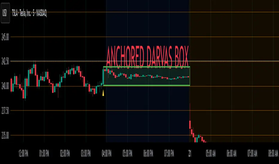
Anchored Darvas Box## ANCHORED DARVAS BOX
---
### OVERVIEW
**Anchored Darvas Box** lets you drop a single timestamp on your chart and build a Darvas-style consolidation zone forward from that exact candle. The indicator freezes the first user-defined number of bars to establish the range, verifies that price respects that range for another user-defined number of bars, then waits for the first decisive breakout. The resulting rectangle captures every tick of the accumulation phase and the exact moment of expansion—no manual drawing, complete timestamp precision.
---
### HISTORICAL BACKGROUND
Nicolas Darvas’s 1950s box theory tracked institutional accumulation by hand-drawing rectangles around tight price ranges. A trade was triggered only when price escaped the rectangle.
The anchored version preserves Darvas’s logic but pins the entire sequence to a user-chosen candle: perfect for analysing a market open, an earnings release, FOMC minute, or any other catalytic bar.
---
### ALGORITHM DETAIL
1. **ANCHOR BAR**
*You provide a timestamp via the settings panel.* The script waits until the chart reaches that bar and records its index as **startBar**.
2. **RANGE DEFINITION — BARS 1-7**
• `rangeHigh` = highest high of bars 1-7 plus optional tolerance.
• `rangeLow` = lowest low of bars 1-7 minus optional tolerance.
3. **RANGE VALIDATION — BARS 8-14**
• Price must stay inside ` `.
• Any violation aborts the test; no box is created.
4. **ARMED STATE**
• If bars 8-14 hold the range, two live guide-lines appear:
– **Green** at `rangeHigh`
– **Red** at `rangeLow`
• The script is now “armed,” waiting indefinitely for the first true breakout.
5. **BREAKOUT & BOX CREATION**
• **Up breakout** =`high > rangeHigh` → rectangle drawn in **green**.
• **Down breakout**=`low < rangeLow` → rectangle drawn in **red**.
• Box extends from **startBar** to the breakout bar and never updates again.
• Optional labels print the dollar and percentage height of the box at its left edge.
6. **OPTIONAL COOLDOWN**
• After the box is painted the script can stay silent for a user-defined number of bars, letting you study the fallout without another range immediately arming on top of it.
---
### INPUT PARAMETERS
• **ANCHOR TIME** – Precise yyyy-mm-dd HH:MM:SS that seeds the sequence.
• **BARS TO DEFINE RANGE** – Default 7; affects both definition and validation windows.
• **OPTIONAL TOLERANCE** – Absolute price buffer to ignore micro-wicks.
• **COOLDOWN BARS AFTER BREAKOUT** – Pause length before the indicator is allowed to re-anchor (set to zero to disable).
• **SHOW BOX DISTANCE LABELS** – Toggle to print Δ\$ and Δ% on every completed box.
---
### USER WORKFLOW
1. Add the indicator, open settings, and set **ANCHOR TIME** to the candle you care about (e.g., “2025-04-23 09:30:00” for NYSE open).
2. Watch live as the script:
– Paints the seven-bar range.
– Draws validation lines.
– Locks in the box on breakout.
3. Use the box boundaries as structural stops, targets, or context for further trades.
---
### PRACTICAL APPLICATIONS
• **OPENING RANGE BREAKOUTS** – Anchor at the first second of the session; capture the initial 7-bar range and trade the first clean break.
• **EVENT STUDIES** – Anchor at a news candle to measure immediate post-event volatility.
• **VOLUME PROFILE FUSION** – Combine the anchored box with VPVR to see if the breakout occurs at a high-volume node or a low-liquidity pocket.
• **RISK DISCIPLINE** – Stop-loss can sit just inside the opposite edge of the anchored range, enforcing objective risk.
---
### ADVANCED CUSTOMISATION IDEAS
• **MULTIPLE ANCHORS** – Clone the indicator and anchor several boxes (e.g., London open, New York open).
• **DYNAMIC WINDOW** – Switch the 7-bar fixed length to a volatility-scaled length (ATR percentile).
• **STRATEGY WRAPPER** – Turn the indicator into a `strategy{}` script and back-test anchored boxes on decades of data.
---
### FINAL THOUGHTS
Anchored Darvas Boxes give you Darvas’s timeless range-break methodology anchored to any candle of interest—perfect for dissecting openings, economic releases, or your own bespoke “important” bars with laboratory precision.
Express Generator StrategyExpress Generator Strategy
Pine Script™ v6
The Express Generator Strategy is an algorithmic trading system that harnesses confluence from multiple technical indicators to optimize trade entries and dynamic risk management. Developed in Pine Script v6, it is designed to operate within a user-defined backtesting period—ensuring that trades are executed only during chosen historical windows for targeted analysis.
How It Works:
- Entry Conditions:
The strategy relies on a dual confirmation approach:- A moving average crossover system where a fast (default 9-period SMA) crossing above or below a slower (default 21-period SMA) average signals a potential trend reversal.
- MACD confirmation; trades are only initiated when the MACD line crosses its signal line in the direction of the moving average signal.
- An RSI filter refines these signals by preventing entries when the market might be overextended—ensuring that long entries only occur when the RSI is below an overbought level (default 70) and short entries when above an oversold level (default 30).
- Risk Management & Dynamic Position Sizing:
The strategy takes a calculated approach to risk by enabling the adjustment of position sizes using:- A pre-defined percentage of equity risk per trade (default 1%, adjustable between 0.5% to 3%).
- A stop-loss set in pips (default 100 pips, with customizable ranges), which is then adjusted by market volatility measured through the ATR.
- Trailing stops (default 50 pips) to help protect profits as the market moves favorably.
This combination of volatility-adjusted risk and equity-based position sizing aims to harmonize trade exposure with prevailing market conditions.
- Backtest Period Flexibility:
Users can define the start and end dates for backtesting (e.g., January 1, 2020 to December 31, 2025). This ensures that the strategy only opens trades within the intended analysis window. Moreover, if the strategy is still holding a position outside this period, it automatically closes all trades to prevent unwanted exposure.
- Visual Insights:
For clarity, the strategy plots the fast (blue) and slow (red) moving averages directly on the chart, allowing for visual confirmation of crossovers and trend shifts.
By integrating multiple technical indicators with robust risk management and adaptable position sizing, the Express Generator Strategy provides a comprehensive framework for capturing trending moves while prudently managing downside risk. It’s ideally suited for traders looking to combine systematic entries with a disciplined and dynamic risk approach.
