Candle Range Theory | Flux Charts💎 GENERAL OVERVIEW
Introducing our new Candle Range Theory Indicator! This powerful tool offers a strategy built around the Candle Range Theory, which analyzes market movements through the relative size and structure of price candles. For more information about the process, check the "HOW DOES IT WORK" section.
Features of the new Candle Range Theory Indicator :
Implementation of the Candle Range Theory
FVG & Order Block Entry Methods
2 Different TP / SL Methods
Customizable Execution Settings
Customizable Backtesting Dashboard
Alerts for Buy, Sell, TP & SL Signals
📌 HOW DOES IT WORK ?
The Candle Range Theory (CRT) indicator operates by identifying significant price movements through the relative size and structure of candlesticks. A key part of the strategy is determining large candles based on their range compared to the Average True Range (ATR) in a higher timeframe. Once identified, a breakout of either the high wick or the low wick of the large candle is required. This breakout is considered a liquidity grab. After that, the indicator waits for confirmation through Fair Value Gaps (FVGs) or Order Blocks (OBs). The confirmation structure must be the opposite direction of the breakout, for example if the high wick is broken, a bearish FVG is required for the short entry. After a confirmation signal is received, the indicator will trigger entry points based on your chosen entry method (FVG or OB), and exit points will be calculated using either a dynamic ATR-based TP/SL method or fixed percentages. Alerts for Buy, Sell, Take-Proft, and Stop-Loss are available.
🚩 UNIQUENESS
This indicator stands out because it combines two highly effective entry methods: Fair Value Gaps (FVGs) and Order Blocks (OBs). You can choose between these strategies depending on market conditions. Additionally, the dynamic TP/SL system uses the ticker's volatility to automatically calculate stop-loss and take-profit targets. The backtesting dashboard provides metrics about the performance of the indicator. You can use it to tune the settings for best use in the current tiker. The Candle Range Theory approach offers more flexibility compared to traditional indicators, allowing for better customization and control based on your risk tolerance.
⚙️ SETTINGS
1. General Configuration
Higher Timeframe: Customize the higher timeframe for analysis. Recommended combinations include M15 -> H4, H4 -> Daily, Daily -> Weekly, and Weekly -> Monthly.
HTF Candle Size: Define the size of the higher timeframe candles as Big, Normal, or Small to filter valid setups based on their range relative to ATR.
Entry Mode: Choose between FVGs and Order Blocks for your entry triggers.
Require Retracement: Enable this option if you want a retracement to the FVG or OB for entry confirmation.
Show HTF Candle Lines: Toggle to display the higher timeframe candle lines for better visual clarity.
2. Fair Value Gaps
FVG Sensitivity: You may select between Low, Normal, High or Extreme FVG detection sensitivity. This will essentially determine the size of the spotted FVGs, with lower sensitivities resulting in spotting bigger FVGs, and higher sensitivities resulting in spotting all sizes of FVGs.
3. Order Blocks
Swing Length: Swing length is used when finding order block formations. Smaller values will result in finding smaller order blocks.
4. TP / SL
TP / SL Method:
a) Dynamic: The TP / SL zones will be auto-determined by the algorithm based on the Average True Range (ATR) of the current ticker.
b) Fixed : You can adjust the exact TP / SL ratios from the settings below.
Dynamic Risk: The risk you're willing to take if "Dynamic" TP / SL Method is selected. Higher risk usually means a better winrate at the cost of losing more if the strategy fails. This setting is has a crucial effect on the performance of the indicator, as different tickers may have different volatility so the indicator may have increased performance when this setting is correctly adjusted.
Komut dosyalarını "the strat" için ara

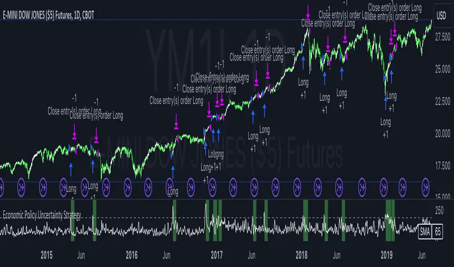
Futures Beta Overview with Different BenchmarksBeta Trading and Its Implementation with Futures
Understanding Beta
Beta is a measure of a security's volatility in relation to the overall market. It represents the sensitivity of the asset's returns to movements in the market, typically benchmarked against an index like the S&P 500. A beta of 1 indicates that the asset moves in line with the market, while a beta greater than 1 suggests higher volatility and potential risk, and a beta less than 1 indicates lower volatility.
The Beta Trading Strategy
Beta trading involves creating positions that exploit the discrepancies between the theoretical (or expected) beta of an asset and its actual market performance. The strategy often includes:
Long Positions on High Beta Assets: Investors might take long positions in assets with high beta when they expect market conditions to improve, as these assets have the potential to generate higher returns.
Short Positions on Low Beta Assets: Conversely, shorting low beta assets can be a strategy when the market is expected to decline, as these assets tend to perform better in down markets compared to high beta assets.
Betting Against (Bad) Beta
The paper "Betting Against Beta" by Frazzini and Pedersen (2014) provides insights into a trading strategy that involves betting against high beta stocks in favor of low beta stocks. The authors argue that high beta stocks do not provide the expected return premium over time, and that low beta stocks can yield higher risk-adjusted returns.
Key Points from the Paper:
Risk Premium: The authors assert that investors irrationally demand a higher risk premium for holding high beta stocks, leading to an overpricing of these assets. Conversely, low beta stocks are often undervalued.
Empirical Evidence: The paper presents empirical evidence showing that portfolios of low beta stocks outperform portfolios of high beta stocks over long periods. The performance difference is attributed to the irrational behavior of investors who overvalue riskier assets.
Market Conditions: The paper suggests that the underperformance of high beta stocks is particularly pronounced during market downturns, making low beta stocks a more attractive investment during volatile periods.
Implementation of the Strategy with Futures
Futures contracts can be used to implement the betting against beta strategy due to their ability to provide leveraged exposure to various asset classes. Here’s how the strategy can be executed using futures:
Identify High and Low Beta Futures: The first step involves identifying futures contracts that have high beta characteristics (more sensitive to market movements) and those with low beta characteristics (less sensitive). For example, commodity futures like crude oil or agricultural products might exhibit high beta due to their price volatility, while Treasury bond futures might show lower beta.
Construct a Portfolio: Investors can construct a portfolio that goes long on low beta futures and short on high beta futures. This can involve trading contracts on stock indices for high beta stocks and bonds for low beta exposures.
Leverage and Risk Management: Futures allow for leverage, which means that a small movement in the underlying asset can lead to significant gains or losses. Proper risk management is essential, using stop-loss orders and position sizing to mitigate the inherent risks associated with leveraged trading.
Adjusting Positions: The positions may need to be adjusted based on market conditions and the ongoing performance of the futures contracts. Continuous monitoring and rebalancing of the portfolio are essential to maintain the desired risk profile.
Performance Evaluation: Finally, investors should regularly evaluate the performance of the portfolio to ensure it aligns with the expected outcomes of the betting against beta strategy. Metrics like the Sharpe ratio can be used to assess the risk-adjusted returns of the portfolio.
Conclusion
Beta trading, particularly the strategy of betting against high beta assets, presents a compelling approach to capitalizing on market inefficiencies. The research by Frazzini and Pedersen emphasizes the benefits of focusing on low beta assets, which can yield more favorable risk-adjusted returns over time. When implemented using futures, this strategy can provide a flexible and efficient means to execute trades while managing risks effectively.
References
Frazzini, A., & Pedersen, L. H. (2014). Betting against beta. Journal of Financial Economics, 111(1), 1-25.
Fama, E. F., & French, K. R. (1992). The cross-section of expected stock returns. Journal of Finance, 47(2), 427-465.
Black, F. (1972). Capital Market Equilibrium with Restricted Borrowing. Journal of Business, 45(3), 444-454.
Ang, A., & Chen, J. (2010). Asymmetric volatility: Evidence from the stock and bond markets. Journal of Financial Economics, 99(1), 60-80.
By utilizing the insights from academic literature and implementing a disciplined trading strategy, investors can effectively navigate the complexities of beta trading in the futures market.

Overnight Positioning w EMA - Strategy [presentTrading]I've recently started researching Market Timing strategies, and it’s proving to be quite an interesting area of study. The idea of predicting optimal times to enter and exit the market, based on historical data and various indicators, brings a dynamic edge to trading. Additionally, it is integrated with the 3commas bot for automated trade execution.
I'm still working on it. Welcome to share your point of view.
█ Introduction and How it is Different
The "Overnight Positioning with EMA " is designed to capitalize on market inefficiencies during the overnight trading period. This strategy takes a position shortly before the market closes and exits shortly after it opens the following day. What sets this strategy apart is the integration of an optional Exponential Moving Average (EMA) filter, which ensures that trades are aligned with the underlying trend. The strategy provides flexibility by allowing users to select between different global market sessions, such as the US, Asia, and Europe.
It is integrated with the 3commas bot for automated trade execution and has a built-in mechanism to avoid holding positions over the weekend by force-closing positions on Fridays before the market closes.
BTCUSD 20 mins Performance
█ Strategy, How it Works: Detailed Explanation
The core logic of this strategy is simple: enter trades before market close and exit them after market open, taking advantage of potential price movements during the overnight period. Here’s how it works in more detail:
🔶 Market Timing
The strategy determines the local market open and close times based on the selected market (US, Asia, Europe) and adjusts entry and exit points accordingly. The entry is triggered a specific number of minutes before market close, and the exit is triggered a specific number of minutes after market open.
🔶 EMA Filter
The strategy includes an optional EMA filter to help ensure that trades are taken in the direction of the prevailing trend. The EMA is calculated over a user-defined timeframe and length. The entry is only allowed if the closing price is above the EMA (for long positions), which helps to filter out trades that might go against the trend.
The EMA formula:
```
EMA(t) = +
```
Where:
- EMA(t) is the current EMA value
- Close(t) is the current closing price
- n is the length of the EMA
- EMA(t-1) is the previous period's EMA value
🔶 Entry Logic
The strategy monitors the market time in the selected timezone. Once the current time reaches the defined entry period (e.g., 20 minutes before market close), and the EMA condition is satisfied, a long position is entered.
- Entry time calculation:
```
entryTime = marketCloseTime - entryMinutesBeforeClose * 60 * 1000
```
🔶 Exit Logic
Exits are triggered based on a specified time after the market opens. The strategy checks if the current time is within the defined exit period (e.g., 20 minutes after market open) and closes any open long positions.
- Exit time calculation:
exitTime = marketOpenTime + exitMinutesAfterOpen * 60 * 1000
🔶 Force Close on Fridays
To avoid the risk of holding positions over the weekend, the strategy force-closes any open positions 5 minutes before the market close on Fridays.
- Force close logic:
isFriday = (dayofweek(currentTime, marketTimezone) == dayofweek.friday)
█ Trade Direction
This strategy is designed exclusively for long trades. It enters a long position before market close and exits the position after market open. There is no shorting involved in this strategy, and it focuses on capturing upward momentum during the overnight session.
█ Usage
This strategy is suitable for traders who want to take advantage of price movements that occur during the overnight period without holding positions for extended periods. It automates entry and exit times, ensuring that trades are placed at the appropriate times based on the market session selected by the user. The 3commas bot integration also allows for automated execution, making it ideal for traders who wish to set it and forget it. The strategy is flexible enough to work across various global markets, depending on the trader's preference.
█ Default Settings
1. entryMinutesBeforeClose (Default = 20 minutes):
This setting determines how many minutes before the market close the strategy will enter a long position. A shorter duration could mean missing out on potential movements, while a longer duration could expose the position to greater price fluctuations before the market closes.
2. exitMinutesAfterOpen (Default = 20 minutes):
This setting controls how many minutes after the market opens the position will be exited. A shorter exit time minimizes exposure to market volatility at the open, while a longer exit time could capture more of the overnight price movement.
3. emaLength (Default = 100):
The length of the EMA affects how the strategy filters trades. A shorter EMA (e.g., 50) reacts more quickly to price changes, allowing more frequent entries, while a longer EMA (e.g., 200) smooths out price action and only allows entries when there is a stronger underlying trend.
The effect of using a longer EMA (e.g., 200) would be:
```
EMA(t) = +
```
4. emaTimeframe (Default = 240):
This is the timeframe used for calculating the EMA. A higher timeframe (e.g., 360) would base entries on longer-term trends, while a shorter timeframe (e.g., 60) would respond more quickly to price movements, potentially allowing more frequent trades.
5. useEMA (Default = true):
This toggle enables or disables the EMA filter. When enabled, trades are only taken when the price is above the EMA. Disabling the EMA allows the strategy to enter trades without any trend validation, which could increase the number of trades but also increase risk.
6. Market Selection (Default = US):
This setting determines which global market's open and close times the strategy will use. The selection of the market affects the timing of entries and exits and should be chosen based on the user's preference or geographic focus.

Martingale with MACD+KDJ opening conditionsStrategy Overview:
This strategy is based on a Martingale trading approach, incorporating MACD and KDJ indicators. It features pyramiding, trailing stops, and dynamic profit-taking mechanisms, suitable for both long and short trades. The strategy increases position size progressively using a Multiplier, a key feature of Martingale systems.
Key Concepts:
Martingale Strategy: A trading system where positions are doubled or increased after a loss to recover previous losses with a single successful trade. In this script, the position size is incremented using a Multiplier for each addition.
Pyramiding: Allows adding to existing trades when market conditions are favorable, enhancing profitability during trends.
Settings:
Basic Inputs:
Initial Order: Defines the starting size of the position.
Default: 150.0
MACD Settings: Customize the fast, slow, and signal smoothing lengths.
Default: Fast Length: 9, Slow Length: 26, Signal Smoothing: 9
KDJ Settings: Customize the length and smoothing parameters for KDJ.
Default: Length: 14, Smooth K: 3, Smooth D: 3
Max Additions: Sets the number of additional positions (pyramiding).
Default: 5 (Min: 1, Max: 10)
Position Sizing: Percent to add to positions on favorable conditions.
Default: 1.0%
Martingale Multiplier:
Add Multiplier: This value controls the scaling of additional positions according to the Martingale principle. After each loss, a new position is added, and its size is increased by the Multiplier factor. For example, with a multiplier of 2, each new addition will be twice as large as the previous one, accelerating recovery if the price moves favorably.
Default: 1.0 (no multiplication)
Can be adjusted up to 10x to aggressively increase position size after losses.
Trade Execution:
Long Trades:
Entry Condition: A long position is opened when the MACD line crosses over the signal line, and the KDJ’s %K crosses above %D.
Additions (Martingale): After the initial long position, new positions are added if the price drops by the defined percentage, and each new addition is increased using the Multiplier. This continues up to the set Max Additions.
Short Trades:
Entry Condition: A short position is opened when the MACD line crosses under the signal line, and the KDJ’s %K crosses below %D.
Additions (Martingale): After the initial short position, new positions are added if the price rises by the defined percentage, and each new addition is increased using the Multiplier.
Exit Conditions:
Take Profit: Exits are triggered when the price reaches the take-profit threshold.
Stop Loss: If the price moves unfavorably, the position will be closed at the set stop-loss level.
Trailing Stop: Adjusts dynamically as the price moves in favor of the trade to lock in profits.
On-Chart Visuals:
Long Signals: Blue triangles below the bars indicate long entries, and green triangles mark additional long positions.
Short Signals: Red triangles above the bars indicate short entries, and orange triangles mark additional short positions.
Information Table:
The strategy displays a table with key metrics:
Open Price: The entry price of the trade.
Average Price: The average price of the current position.
Additions: The number of additional positions taken.
Next Add Price: The price level for the next position.
Take Profit: The price at which profits will be taken.
Stop Loss: The stop-loss level to minimize risk.
Usage Instructions:
Adjust the parameters to your trading style using the input settings.
The Multiplier amplifies your position size after each addition, so use it cautiously, especially in volatile markets.
Monitor the signals and table on the chart for entry/exit decisions and trade management.

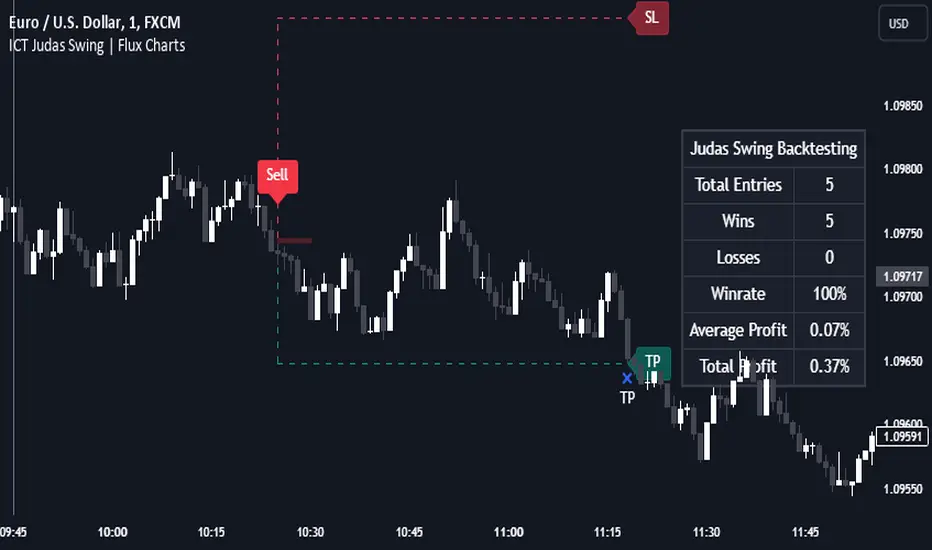
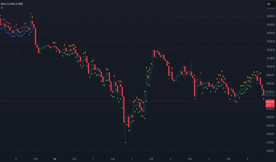
ICT Judas Swing | Flux Charts💎 GENERAL OVERVIEW
Introducing our new ICT Judas Swing Indicator! This indicator is built around the ICT's "Judas Swing" strategy. The strategy looks for a liquidity grab around NY 9:30 session and a Fair Value Gap for entry confirmation. For more information about the process, check the "HOW DOES IT WORK" section.
Features of the new ICT Judas Swing :
Implementation of ICT's Judas Swing Strategy
2 Different TP / SL Methods
Customizable Execution Settings
Customizable Backtesting Dashboard
Alerts for Buy, Sell, TP & SL Signals
📌 HOW DOES IT WORK ?
The strategy begins by identifying the New York session from 9:30 to 9:45 and marking recent liquidity zones. These liquidity zones are determined by locating high and low pivot points: buyside liquidity zones are identified using high pivots that haven't been invalidated, while sellside liquidity zones are found using low pivots. A break of either buyside or sellside liquidity must occur during the 9:30-9:45 session, which is interpreted as a liquidity grab by smart money. The strategy assumes that after this liquidity grab, the price will reverse and move in the opposite direction. For entry confirmation, a fair value gap (FVG) in the opposite direction of the liquidity grab is required. A buyside liquidity grab calls for a bearish FVG, while a sellside grab requires a bullish FVG. Based on the type of FVG—bullish for buys and bearish for sells—the indicator will then generate a Buy or Sell signal.
After the Buy or Sell signal, the indicator immediately draws the take-profit (TP) and stop-loss (SL) targets. The indicator has three different TP & SL modes, explained in the "Settings" section of this write-up.
You can set up alerts for entry and TP & SL signals, and also check the current performance of the indicator and adjust the settings accordingly to the current ticker using the backtesting dashboard.
🚩 UNIQUENESS
This indicator is an all-in-one suit for the ICT's Judas Swing concept. It's capable of plotting the strategy, giving signals, a backtesting dashboard and alerts feature. Different and customizable algorithm modes will help the trader fine-tune the indicator for the asset they are currently trading. Three different TP / SL modes are available to suit your needs. The backtesting dashboard allows you to see how your settings perform in the current ticker. You can also set up alerts to get informed when the strategy is executable for different tickers.
⚙️ SETTINGS
1. General Configuration
Swing Length -> The swing length for pivot detection. Higher settings will result in
FVG Detection Sensitivity -> You may select between Low, Normal, High or Extreme FVG detection sensitivity. This will essentially determine the size of the spotted FVGs, with lower sensitivies resulting in spotting bigger FVGs, and higher sensitivies resulting in spotting all sizes of FVGs.
2. TP / SL
TP / SL Method ->
a) Dynamic: The TP / SL zones will be auto-determined by the algorithm based on the Average True Range (ATR) of the current ticker.
b) Fixed : You can adjust the exact TP / SL ratios from the settings below.
Dynamic Risk -> The risk you're willing to take if "Dynamic" TP / SL Method is selected. Higher risk usually means a better winrate at the cost of losing more if the strategy fails. This setting is has a crucial effect on the performance of the indicator, as different tickers may have different volatility so the indicator may have increased performance when this setting is correctly adjusted.
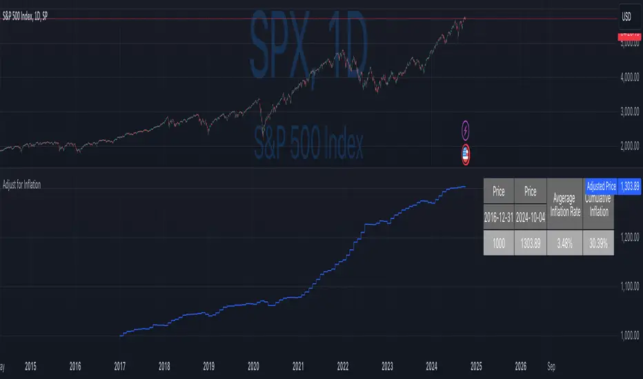
Inflation-Adjusted Price IndicatorThis indicator allows traders to adjust historical prices for inflation using customizable CPI data. The script computes the adjusted price by selecting a reference date, the original price, and the CPI source (US CPI or custom input) and plots it as a line on the chart. Additionally, a table summarizes the adjusted price values and average and total inflation rates.
While the indicator serves as a standalone tool to understand inflation's impact on prices, it is a supportive element in more advanced trading strategies requiring accurate analysis of inflation-adjusted data.
Disclaimer
Please remember that past performance may not be indicative of future results.
Due to various factors, including changing market conditions, the strategy may no longer perform as well as in historical backtesting.
This post and the script don’t provide any financial advice.
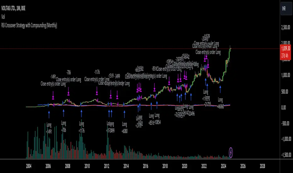
RSI Crossover Strategy with Compounding (Monthly)Explanation of the Code:
Initial Setup:
The strategy initializes with a capital of 100,000.
Variables track the capital and the amount invested in the current trade.
RSI Calculation:
The RSI and its SMA are calculated on the monthly timeframe using request.security().
Entry and Exit Conditions:
Entry: A long position is initiated when the RSI is above its SMA and there’s no existing position. The quantity is based on available capital.
Exit: The position is closed when the RSI falls below its SMA. The capital is updated based on the net profit from the trade.
Capital Management:
After closing a trade, the capital is updated with the net profit plus the initial investment.
Plotting:
The RSI and its SMA are plotted for visualization on the chart.
A label displays the current capital.
Notes:
Test the strategy on different instruments and historical data to see how it performs.
Adjust parameters as needed for your specific trading preferences.
This script is a basic framework, and you might want to enhance it with risk management, stop-loss, or take-profit features as per your trading strategy.
Feel free to modify it further based on your needs!
KAMA Cloud STIndicator:
Description:
The KAMA Cloud indicator is a sophisticated trading tool designed to provide traders with insights into market trends and their intensity. This indicator is built on the Kaufman Adaptive Moving Average (KAMA), which dynamically adjusts its sensitivity to filter out market noise and respond to significant price movements. The KAMA Cloud leverages multiple KAMAs to gauge trend direction and strength, offering a visual representation that is easy to interpret.
How It Works:
The KAMA Cloud uses twenty different KAMA calculations, each set to a distinct lookback period ranging from 5 to 100. These KAMAs are calculated using the average of the open, high, low, and close prices (OHLC4), ensuring a balanced view of price action. The relative positioning of these KAMAs helps determine the direction of the market trend and its momentum.
By measuring the cumulative relative distance between these KAMAs, the indicator effectively assesses the overall trend strength, akin to how the Average True Range (ATR) measures market volatility. This cumulative measure helps in identifying the trend’s robustness and potential sustainability.
The visualization component of the KAMA Cloud is particularly insightful. It plots a 'cloud' formed between the base KAMA (set at a 100-period lookback) and an adjusted KAMA that incorporates the cumulative relative distance scaled up. This cloud changes color based on the trend direction — green for upward trends and red for downward trends, providing a clear, visual representation of market conditions.
How the Strategy Works:
The KAMA Cloud ST strategy employs multiple KAMA calculations with varying lengths to capture the nuances of market trends. It measures the relative distances between these KAMAs to determine the trend's direction and strength, much like the original indicator. The strategy enhances decision-making by plotting a 'cloud' formed between the base KAMA (set to a 100-period lookback) and an adjusted KAMA that scales according to the cumulative relative distance of all KAMAs.
Key Components of the Strategy:
Multiple KAMA Layers: The strategy calculates KAMAs for periods ranging from 5 to 100 to analyze short to long-term market trends.
Dynamic Cloud: The cloud visually represents the trend’s strength and direction, updating in real-time as the market evolves.
Signal Generation: Trade signals are generated based on the orientation of the cloud relative to a smoothed version of the upper KAMA boundary. Long positions are initiated when the market trend is upward, and the current cloud value is above its smoothed average. Conversely, positions are closed when the trend reverses, indicated by the cloud falling below the smoothed average.
Suggested Usage:
Market: Stocks, not cryptocurrency
Timeframe: 1 Hour
Indicator:

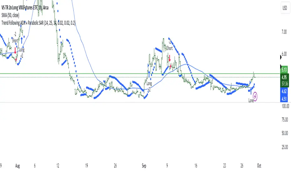
Trend Following ADX + Parabolic SAR### Strategy Description: Trend Following using **ADX** and **Parabolic SAR**
This strategy is designed to follow market trends using two popular indicators: **Average Directional Index (ADX)** and **Parabolic SAR**. The strategy attempts to enter trades when the market shows a strong trend (using ADX) and confirms the trend direction using the Parabolic SAR. Here's a breakdown:
### Key Indicators:
1. **ADX (Average Directional Index)**:
- **Purpose**: ADX measures the strength of a trend, regardless of direction.
- **Usage**: The strategy uses ADX to confirm that the market is trending. When ADX is above a certain threshold (e.g., 25), it indicates a strong trend.
- **Directional Indicators**:
- **DI+ (Directional Indicator Plus)**: Indicates upward movement strength.
- **DI- (Directional Indicator Minus)**: Indicates downward movement strength.
2. **Parabolic SAR**:
- **Purpose**: Parabolic SAR is a trend-following indicator used to identify potential reversals in the price direction.
- **Usage**: It provides specific price points above or below which the strategy confirms buy or sell signals.
### Strategy Logic:
#### **Entry Conditions**:
1. **Long Position** (Buy):
- **ADX** is above the threshold (default: 25), indicating a strong trend.
- **DI+ > DI-**, indicating the upward trend is stronger than the downward.
- The price is above the **Parabolic SAR** level, confirming the upward trend.
2. **Short Position** (Sell):
- **ADX** is above the threshold (default: 25), indicating a strong trend.
- **DI- > DI+**, indicating the downward trend is stronger than the upward.
- The price is below the **Parabolic SAR** level, confirming the downward trend.
#### **Exit Conditions**:
- Positions are closed when an opposite signal is detected.
- For example, if a long position is open and the conditions for a short position are met, the long position is closed, and a short position is opened.
### Parameters:
1. **ADX Period**: Defines the length of the period for the ADX calculation (default: 14).
2. **ADX Threshold**: The minimum value of ADX to confirm a strong trend (default: 25).
3. **Parabolic SAR Start**: The initial step for the SAR (default: 0.02).
4. **Parabolic SAR Increment**: The step increment for SAR (default: 0.02).
5. **Parabolic SAR Max**: The maximum step for SAR (default: 0.2).
### Example Trade Flow:
#### **Long Trade**:
1. ADX > 25, confirming a strong trend.
2. DI+ > DI-, indicating the market is trending upward.
3. The price is above the Parabolic SAR, confirming the upward direction.
4. **Action**: Enter a long (buy) position.
5. Exit the long position when a short signal is triggered (i.e., DI- > DI+, price below Parabolic SAR).
#### **Short Trade**:
1. ADX > 25, confirming a strong trend.
2. DI- > DI+, indicating the market is trending downward.
3. The price is below the Parabolic SAR, confirming the downward direction.
4. **Action**: Enter a short (sell) position.
5. Exit the short position when a long signal is triggered (i.e., DI+ > DI-, price above Parabolic SAR).
### Strengths of the Strategy:
- **Trend-Following**: It performs well in markets with strong trends, whether upward or downward.
- **Dual Confirmation**: The combination of ADX and Parabolic SAR reduces false signals by ensuring both trend strength and direction are considered before entering a trade.
### Weaknesses:
- **Range-Bound Markets**: This strategy may perform poorly in choppy, non-trending markets because both ADX and SAR are trend-following indicators.
- **Lagging Nature**: Since both ADX and SAR are lagging indicators, the strategy may enter trades after the trend has already started, potentially missing early profits.
### Customization:
- **ADX Threshold**: You can increase the threshold if you only want to trade in very strong trends, or lower it to capture more moderate trends.
- **SAR Parameters**: Adjusting the SAR `start`, `increment`, and `max` values will make the Parabolic SAR more or less sensitive to price changes.
### Summary:
This strategy combines the ADX and Parabolic SAR to take advantage of strong market trends. By confirming both trend strength (ADX) and trend direction (Parabolic SAR), it aims to enter high-probability trades in trending markets while minimizing false signals. However, it may struggle in sideways or non-trending markets.
For Educational purposes only !!!
Commitment of Trader %R StrategyThis Pine Script strategy utilizes the Commitment of Traders (COT) data to inform trading decisions based on the Williams %R indicator. The script operates in TradingView and includes various functionalities that allow users to customize their trading parameters.
Here’s a breakdown of its key components:
COT Data Import:
The script imports the COT library from TradingView to access historical COT data related to different trader groups (commercial hedgers, large traders, and small traders).
User Inputs:
COT data selection mode (e.g., Auto, Root, Base currency).
Whether to include futures, options, or both.
The trader group to analyze.
The lookback period for calculating the Williams %R.
Upper and lower thresholds for triggering trades.
An option to enable or disable a Simple Moving Average (SMA) filter.
Williams %R Calculation: The script calculates the Williams %R value, which is a momentum indicator that measures overbought or oversold levels based on the highest and lowest prices over a specified period.
SMA Filter: An optional SMA filter allows users to limit trades to conditions where the price is above or below the SMA, depending on the configuration.
Trade Logic: The strategy enters long positions when the Williams %R value exceeds the upper threshold and exits when the value falls below it. Conversely, it enters short positions when the Williams %R value is below the lower threshold and exits when the value rises above it.
Visual Elements: The script visually indicates the Williams %R values and thresholds on the chart, with the option to plot the SMA if enabled.
Commitment of Traders (COT) Data
The COT report is a weekly publication by the Commodity Futures Trading Commission (CFTC) that provides a breakdown of open interest positions held by different types of traders in the U.S. futures markets. It is widely used by traders and analysts to gauge market sentiment and potential price movements.
Data Collection: The COT data is collected from futures commission merchants and is published every Friday, reflecting positions as of the previous Tuesday. The report categorizes traders into three main groups:
Commercial Traders: These are typically hedgers (like producers and processors) who use futures to mitigate risk.
Non-Commercial Traders: Often referred to as speculators, these traders do not have a commercial interest in the underlying commodity but seek to profit from price changes.
Non-reportable Positions: Small traders who do not meet the reporting threshold set by the CFTC.
Interpretation:
Market Sentiment: By analyzing the positions of different trader groups, market participants can gauge sentiment. For instance, if commercial traders are heavily short, it may suggest they expect prices to decline.
Extreme Positions: Some traders look for extreme positions among non-commercial traders as potential reversal signals. For example, if speculators are overwhelmingly long, it might indicate an overbought condition.
Statistical Insights: COT data is often used in conjunction with technical analysis to inform trading decisions. Studies have shown that analyzing COT data can provide valuable insights into future price movements (Lund, 2018; Hurst et al., 2017).
Scientific References
Lund, J. (2018). Understanding the COT Report: An Analysis of Speculative Trading Strategies.
Journal of Derivatives and Hedge Funds, 24(1), 41-52. DOI:10.1057/s41260-018-00107-3
Hurst, B., O'Neill, R., & Roulston, M. (2017). The Impact of COT Reports on Futures Market Prices: An Empirical Analysis. Journal of Futures Markets, 37(8), 763-785.
DOI:10.1002/fut.21849
Commodity Futures Trading Commission (CFTC). (2024). Commitment of Traders. Retrieved from CFTC Official Website.

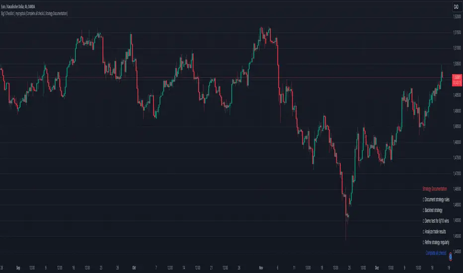
Big 5 Checklist | XEONEDIAThe Big 5 Checklist | XEONEDIA indicator is a powerful trading tool designed to help traders prepare their trading decisions in a structured and effective manner. The indicator encompasses five key areas:
Strategy Documentation :
✅ Ensure that the trading strategy is clearly defined and documented.
✅ Conduct backtesting.
✅ Perform demo testing with an 80% success rate.
✅ Analyze trading results.
✅ Regularly refine the strategy.
Risk Management :
✅ Minimize financial losses and ensure responsible trading.
✅ Set a risk limit of 1-2%.
✅ Use stop-loss orders.
✅ Ensure a risk-reward ratio of at least 2:1.
✅ Adjust position sizes.
Technical Analysis :
✅ Evaluate charts and indicators to identify trading opportunities.
✅ Identify support and resistance levels.
✅ Use technical indicators (e.g., RSI).
✅ Set entry and exit points.
✅ Establish alerts for specific market conditions.
Market Conditions :
✅ Consider external factors that may influence trading.
✅ Monitor the economic calendar.
✅ Apply fundamental analysis.
✅ Observe market volatility.
✅ Analyze global trends.
Psychological Management :
✅ Control emotions and mindset during trading.
✅ Adhere to the trading plan.
✅ Manage emotions while trading.
✅ Set realistic expectations.
✅ Take regular mental breaks.
Mastercheck
The Mastercheck provides a digital checklist where traders can track their progress live. Users can make their own notes and view their checklist on any TradingView device, ensuring they stay informed about their trading readiness and can make adjustments in real-time. ✅
Overall, the Big 5 Checklist | XEONEDIA indicator helps minimize risks and maximize the chances of successful trades by promoting systematic and comprehensive trading preparation.
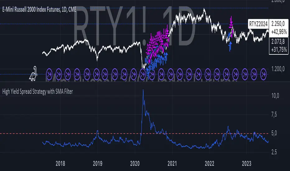
High Yield Spread Strategy with SMA FilterThis Pine Script strategy is designed for statistical analysis and research purposes only, not for live trading or financial decision-making. The script evaluates the relationship between financial volatility (measured by either the VIX or the High Yield Spread) and market positioning strategies (long or short) based on user-defined conditions. Specifically, it allows users to test the assumption that elevated levels of VIX or the High Yield Spread may justify short positions in the market—a widely held belief in financial circles—but this script demonstrates that shorting is not always the optimal choice, even under these conditions.
Key Components:
1. High Yield Spread and VIX:
• High Yield Spread is the difference between the yields of corporate high-yield (or “junk”) bonds and U.S. Treasury securities. A rising spread often reflects increased market risk perception.
• VIX (Volatility Index) is often referred to as the market’s “fear gauge.” Higher VIX levels usually indicate heightened market uncertainty or expected volatility.
2. Strategy Logic:
• The script allows users to specify a threshold for the VIX or High Yield Spread, and it automatically evaluates if the spread exceeds this level, which traditionally would suggest an environment for higher market risk and thus potentially favoring short trades.
• However, the strategy provides flexibility to enter long or short positions, even in a high-risk environment, emphasizing that a high VIX or High Yield Spread does not always warrant shorting.
3. SMA Filter:
• A Simple Moving Average (SMA) filter can be applied to the price data, where positions are only entered if the price is above or below the SMA (depending on the trade direction). This adds a technical component to the strategy, incorporating price trends into decision-making.
4. Hold Duration:
• The script also allows users to define how long to hold a position after entering, enabling an analysis of different timeframes.
Theoretical Background:
The traditional belief that high VIX or High Yield Spreads favor short positions is not universally supported by research. While a spike in the VIX or credit spreads is often associated with increased market risk, research suggests that excessive volatility does not always lead to negative returns. In fact, high volatility can sometimes signal an approaching market rebound.
For example:
• Studies have shown that long-term investments during periods of heightened volatility can yield favorable returns due to mean reversion. Whaley (2000) notes that VIX spikes are often followed by market recoveries as volatility tends to revert to its mean over time .
• Research by Blitz and Vliet (2007) highlights that low-volatility stocks have historically outperformed high-volatility stocks, suggesting that volatility may not always predict negative returns .
• Furthermore, credit spreads can widen in response to broader market stress, but these may overshoot the actual credit risk, presenting opportunities for long positions when spreads are high and risk premiums are mispriced .
Educational Purpose:
The goal of this script is to challenge assumptions about shorting during volatile periods, showing that long positions can be equally, if not more, effective during market stress. By incorporating an SMA filter and customizable logic for entering trades, users can test different hypotheses regarding the effectiveness of both long and short positions under varying market conditions.
Note: This strategy is not intended for live trading and should be used solely for educational and statistical exploration. Misinterpreting financial indicators can lead to incorrect investment decisions, and it is crucial to conduct comprehensive research before trading.
References:
1. Whaley, R. E. (2000). “The Investor Fear Gauge”. The Journal of Portfolio Management, 26(3), 12-17.
2. Blitz, D., & van Vliet, P. (2007). “The Volatility Effect: Lower Risk Without Lower Return”. Journal of Portfolio Management, 34(1), 102-113.
3. Bhamra, H. S., & Kuehn, L. A. (2010). “The Determinants of Credit Spreads: An Empirical Analysis”. Journal of Finance, 65(3), 1041-1072.
This explanation highlights the academic and research-backed foundation of the strategy and the nuances of volatility, while cautioning against the assumption that high VIX or High Yield Spread always calls for shorting.
ETH Signal 15m
This strategy uses the Supertrend indicator combined with RSI to generate buy and sell signals, with stop loss (SL) and take profit (TP) conditions based on ATR (Average True Range). Below is a detailed explanation of each part:
1. General Information BINANCE:ETHUSDT.P
Strategy Name: "ETH Signal 15m"
Designed for use on the 15-minute time frame for the ETH pair.
Default capital allocation is 15% of total equity for each trade.
2. Backtest Period
start_time and end_time: Define the start and end time of the backtest period.
start_time = 2024-08-01: Start date of the backtest.
end_time = 2054-01-01: End date of the backtest.
The strategy will only run when the current time falls within this specified range.
3. Supertrend Indicator
Supertrend is a trend-following indicator that provides buy or sell signals based on the direction of price changes.
factor = 2.76: The multiplier used in the Supertrend calculation (increasing this value makes the Supertrend less sensitive to price movements).
atrPeriod = 12: Number of periods used to calculate ATR.
Output:
direction: Determines the buy/sell direction based on Supertrend.
If direction decreases, it signals a buy (Long).
If direction increases, it signals a sell (Short).
4. RSI Indicator
RSI (Relative Strength Index) is a momentum indicator, often used to identify overbought or oversold conditions.
rsiLength = 12: Number of periods used to calculate RSI.
rsiOverbought = 70: RSI level considered overbought.
rsiOversold = 30: RSI level considered oversold.
5. Entry Conditions
Long Entry:
Supertrend gives a buy signal (ta.change(direction) < 0).
RSI must be below the overbought level (rsi < rsiOverbought).
Short Entry:
Supertrend gives a sell signal (ta.change(direction) > 0).
RSI must be above the oversold level (rsi > rsiOversold).
The strategy will only execute trades if the current time is within the backtest period (in_date_range).
6. Stop Loss (SL) and Take Profit (TP) Conditions
ATR (Average True Range) is used to calculate the distance for Stop Loss and Take Profit based on price volatility.
atr = ta.atr(atrPeriod): ATR is calculated using 12 periods.
Stop Loss and Take Profit are calculated as follows:
Long Trade:
Stop Loss: Set at close - 4 * atr (current price minus 4 times the ATR).
Take Profit: Set at close + 2 * atr (current price plus 2 times the ATR).
Short Trade:
Stop Loss: Set at close + 4 * atr (current price plus 4 times the ATR).
Take Profit: Set at close - 2.237 * atr (current price minus 2.237 times the ATR).
Summary:
This strategy enters a Long trade when the Supertrend indicates an upward trend and RSI is not in the overbought region. Conversely, a Short trade is entered when Supertrend signals a downtrend, and RSI is not oversold.
The trade is exited when the price reaches the Stop Loss or Take Profit levels, which are determined based on price volatility (ATR).
Disclaimer:
The content provided in this strategy is for informational and educational purposes only. It is not intended as financial, investment, or trading advice. Trading in cryptocurrency, stocks, or any financial markets involves significant risk, and you may lose more than your initial investment. Past performance is not indicative of future results, and no guarantee of profit can be made. You should consult with a professional financial advisor before making any investment decisions. The creator of this strategy is not responsible for any financial losses or damages incurred as a result of following this strategy. All trades are executed at your own risk.

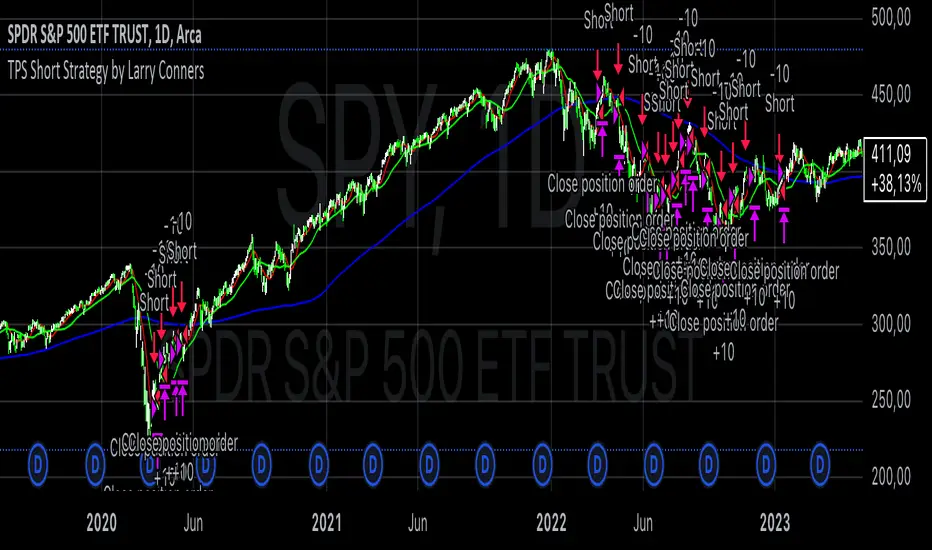
TPS Short Strategy by Larry ConnersThe TPS Short strategy aims to capitalize on extreme overbought conditions in an ETF by employing a scaling-in approach when certain technical indicators signal potential reversals. The strategy is designed to short the ETF when it is deemed overextended, based on the Relative Strength Index (RSI) and moving averages.
Components:
200-Day Simple Moving Average (SMA):
Purpose: Acts as a long-term trend filter. The ETF must be below its 200-day SMA to be eligible for shorting.
Rationale: The 200-day SMA is widely used to gauge the long-term trend of a security. When the price is below this moving average, it is often considered to be in a downtrend (Tushar S. Chande & Stanley Kroll, "The New Technical Trader: Boost Your Profit by Plugging Into the Latest Indicators").
2-Period RSI:
Purpose: Measures the speed and change of price movements to identify overbought conditions.
Criteria: Short 10% of the position when the 2-period RSI is above 75 for two consecutive days.
Rationale: A high RSI value (above 75) indicates that the ETF may be overbought, which could precede a price reversal (J. Welles Wilder, "New Concepts in Technical Trading Systems").
Scaling-In Mechanism:
Purpose: Gradually increase the short position as the ETF price rises beyond previous entry points.
Scaling Strategy:
20% more when the price is higher than the first entry.
30% more when the price is higher than the second entry.
40% more when the price is higher than the third entry.
Rationale: This incremental approach allows for an increased position size in a worsening trend, potentially increasing profitability if the trend continues to align with the strategy’s premise (Marty Schwartz, "Pit Bull: Lessons from Wall Street's Champion Day Trader").
Exit Conditions:
Criteria: Close all positions when the 2-period RSI drops below 30 or the 10-day SMA crosses above the 30-day SMA.
Rationale: A low RSI value (below 30) suggests that the ETF may be oversold and could be poised for a rebound, while the SMA crossover indicates a potential change in the trend (Martin J. Pring, "Technical Analysis Explained").
Risks and Considerations:
Market Risk:
The strategy assumes that the ETF will continue to decline once shorted. However, markets can be unpredictable, and price movements might not align with the strategy's expectations, especially in a volatile market (Nassim Nicholas Taleb, "The Black Swan: The Impact of the Highly Improbable").
Scaling Risks:
Scaling into a position as the price increases may increase exposure to adverse price movements. This method can amplify losses if the market moves against the position significantly before any reversal occurs.
Liquidity Risk:
Depending on the ETF’s liquidity, executing large trades in increments might affect the price and increase trading costs. It is crucial to ensure that the ETF has sufficient liquidity to handle large trades without significant slippage (James Altucher, "Trade Like a Hedge Fund").
Execution Risk:
The strategy relies on timely execution of trades based on specific conditions. Delays or errors in order execution can impact performance, especially in fast-moving markets.
Technical Indicator Limitations:
Technical indicators like RSI and SMA are based on historical data and may not always predict future price movements accurately. They can sometimes produce false signals, leading to potential losses if used in isolation (John Murphy, "Technical Analysis of the Financial Markets").
Conclusion
The TPS Short strategy utilizes a combination of long-term trend filtering, overbought conditions, and incremental shorting to potentially profit from price reversals. While the strategy has a structured approach and leverages well-known technical indicators, it is essential to be aware of the inherent risks, including market volatility, liquidity issues, and potential limitations of technical indicators. As with any trading strategy, thorough backtesting and risk management are crucial to its successful implementation.
Descriptive Backtesting Framework (DBF)As the name suggests, this is a backtesting framework made to offer full backtesting functionality to any custom indicator in a visually descriptive way.
Any trade taken will be very clear to visualize on the chart and the equity line will be updated live allowing us to use the REPLAY feature to view the strategy performing in real time.
Stops and Targets will also get draw on the chart with labels and tooltips and there will be a table on the top right corner displaying lots of descriptive metrics to measure your strategy's performance.
IF YOU DECIDE TO USE THIS FRAMEWORK, PLEASE READ **EVERYTHING** BELOW
HOW TO USE IT
Step 1 - Insert Your Strategy Indicators:
Inside this framework's code, right at the beginning, you will find a dedicated section where you can manually insert any set of indicators you desire.
Just replace the example code in there with your own strategy indicators.
Step 2 - Specify The Conditions To Take Trades:
After that, there will be another section where you need to specify your strategy's conditions to enter and exit trades.
When met, those conditions will fire the trading signals to the trading engine inside the framework.
If you don't wish to use some of the available signals, please just assign false to the signal.
DO NOT DELETE THE SIGNAL VARIABLES
Step 3 - Specify Entry/Exit Prices, Stops & Targets:
Finally you'll reach the last section where you'll be able to specify entry/exit prices as well as add stops and targets.
On most cases, it's easier and more reliable to just use the close price to enter and exit trades.
If you decide to use the open price instead, please remember to change step 2 so that trades are taken on the open price of the next candle and not the present one to avoid the look ahead bias.
Stops and targets can be set in any way you want.
Also, please don't forget to update the spread. If your broker uses commissions instead of spreads or a combination of both, you'll need to manually incorporate those costs in this step.
And that's it! That's all you have to do.
Below this section you'll now see a sign warning you about not making any changes to the code below.
From here on, the framework will take care of executing the trades and calculating the performance metrics for you and making sure all calculations are consistent.
VISUAL FEATURES:
Price candles get painted according to the current trade.
They will be blue during long trades, purple on shorts and white when no trade is on.
When the framework receives the signals to start or close a trade, it will display those signals as shapes on the upper and lower limits of the chart:
DIAMOND: represents a signal to open a trade, the trade direction is represented by the shape's color;
CROSS: means a stop loss was triggered;
FLAG: means a take profit was triggered;
CIRCLE: means an exit trade signal was fired;
Hovering the mouse over the trade labels will reveal:
Asset Quantity;
Entry/Exit Prices;
Stops & Targets;
Trade Profit;
Profit As Percentage Of Trade Volume;
**Please note that there's a limit as to how many labels can be drawn on the chart at once.**
If you which to see labels from the beginning of the chart, you'll probably need to use the replay feature.
PERFORMANCE TABLE:
The performance table displays several performance metrics to evaluate the strategy.
All the performance metrics here are calculated by the framework. It does not uses the oficial pine script strategy tester.
All metrics are calculated in real time. If using the replay feature, they will be updated up to the last played bar.
Here are the available metrics and their definition:
INITIAL EQUITY: the initial amount of money we had when the strategy started, obviously...;
CURRENT EQUITY: the amount of money we have now. If using the replay feature, it will show the current equity up to the last bar played. The number on it's right side shows how many times our equity has been multiplied from it's initial value;
TRADE COUNT: how many trades were taken;
WIN COUNT: how many of those trades were wins. The percentage at the right side is the strategy WIN RATE;
AVG GAIN PER TRADE: the average percentage gain per trade. Very small values can indicate a fragile strategy that can behave in unexpected ways under high volatility conditions;
AVG GAIN PER WIN: the average percentage gain of trades that were profitable;
AVG GAIN PER LOSS: the average percentage loss on trades that were not profitable;
EQUITY MAX DD: the maximum drawdown experienced by our equity during the entire strategy backtest;
TRADE MAX DD: the maximum drawdown experienced by our equity after one single trade;
AVG MONTHLY RETURN: the compound monthly return that our strategy was able to create during the backtested period;
AVG ANNUAL RETURN: this is the strategy's CAGR (compound annual growth rate);
ELAPSED MONTHS: number of months since the backtest started;
RISK/REWARD RATIO: shows how profitable the strategy is for the amount of risk it takes. Values above 1 are very good (and rare). This is calculated as follows: (Avg Annual Return) / mod(Equity Max DD). Where mod() is the same as math.abs();
AVAILABLE SETTINGS:
SPREAD: specify your broker's asset spread
ENABLE LONGS / SHORTS: you can keep both enable or chose to take trades in only one direction
MINIMUM BARS CLOSED: to avoid trading before indicators such as a slow moving average have had time to populate, you can manually set the number of bars to wait before allowing trades.
INITIAL EQUITY: you can specify your starting equity
EXPOSURE: is the percentage of equity you wish to risk per trade. When using stops, the strategy will automatically calculate your position size to match the exposure with the stop distance. If you are not using stops then your trade volume will be the percentage of equity specified here. 100 means you'll enter trades with all your equity and 200 means you'll use a 2x leverage.
MAX LEVERAGE ALLOWED: In some situations a short stop distance can create huge levels of leverage. If you want to limit leverage to a maximum value you can set it here.
SEVERAL PLOTTING OPTIONS: You'll be able to specify which of the framework visuals you wish to see drawn on the chart.
FRAMEWORK **LIMITATIONS**:
When stop and target are both triggered in the same candle, this framework isn't able to enter faster timeframes to check which one was triggered first, so it will take the pessimistic assumption and annul the take profit signal;
This framework doesn't support pyramiding;
This framework doesn't support both long and short positions to be active at the same time. So for example, if a short signal is received while a long trade is open, the framework will close the long trade and then open a short trade;
FINAL CONSIDERATIONS:
I've been using this framework for a good time and I find it's better to use and easier to analyze a strategy's performance then relying on the oficial pine script strategy tester. However, I CANNOT GUARANTEE IT TO BE BUG FREE.
**PLEASE PERFORM A MANUAL BACKTEST BEFORE USING ANY STRATEGY WITH REAL MONEY**

Potential Divergence Checker#### Key Features
1. Potential Divergence Signals:
Potential divergences can signal a change in price movement before it occurs. This indicator identifies potential divergences instead of waiting for full confirmation, allowing it to detect signs of divergence earlier than traditional methods. This provides more flexible entry points and can act as a broader filter for potential setups.
2. Exposing Signals for External Use:
One of its advanced features is the ability to expose signals for use in other scripts. This allows users to integrate divergence signals and related entry/exit points into custom strategies or automated systems.
3. Custom Entry/Exit Timing Based on Years and Days:
The indicator provides entry and exit signals based on years and days, which could be useful for time-specific market behavior, long-term trades, and back testing.
#### Basic Usage
This indicator can check for all types of potential divergences: bullish, hidden bullish, bearish, hidden bearish. All you need to do is choose the type you want to check for under “DIVERGENCE TYPE” in the settings. On the chart, potential bullish divergences will show up as triangles below the price candles. one the chart potential bearish divergences will show up as upside down triangles above the price candles
#### Signals for Advanced Usage
You can use this indicator as a source in other indicators or strategies using the following information:
“ PD: Bull divergence signal ” will return “1” when a divergence is present and “0” when not present
“ PD: HBull divergence(hidden bull) signal ” will return “1” when a divergence is present and “0” when not present
“ PD: Bear divergence signal ” will return “1” when a divergence is present and “0” when not present
“ PD: HBear divergence(hidden bear) signal ” will return “1” when a divergence is present and “0” when not present
“ PD: enter ” signal will return a “1” when both the days and years criteria in the “entry filter settings” are met and “0” when not met.
“ PD: exit ” signal will return a “1” when the days criteria in the “exit filter settings” are met and “0” when not met.
#### Examples of Using Signals
1. If you are testing a long strategy for Bitcoin and do not want it to run during bear market years(e.g., the second year after a US presidential election), you can enable the “year and day filter for entry,” uncheck the following years in the settings: 2010, 2014, 2018, 2022, 2026, and reference the signal below in our strategy
signal: “ PD: enter ”
2. Let’s say you have a good long strategy, but want to make it a bit more profitable, you can tell the strategy not to run on days where there is potential bearish divergence and have it only run on more profitable days using these signals and the appropriate settings in the indicator
signal: “ PD: Bear divergence signal ” will return a ‘0’ with no bearish divergence present
signal: “ PD: enter ” will return a “1” if the entry falls on a specific, more profitable day chosen in the settings
#### Disclaimer
The "Potential Divergence Checker" indicator is a tool designed to identify potential market signals. It may have bugs and not do what it should do. It is not a guarantee of future trading performance, and users should exercise caution when making trading decisions based on its outputs. Always perform your own research and consider consulting with a financial advisor before making any investment decisions. Trading involves significant risk, and past performance is not indicative of future results.
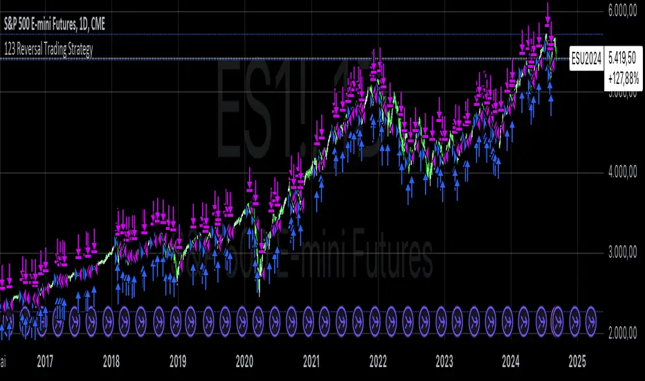
123 Reversal Trading StrategyThe 123 Reversal Trading Strategy is a technical analysis approach that seeks to identify potential reversal points in the market by analyzing price patterns. This Pine Script™ code implements a version of this strategy, and here’s a detailed description:
Strategy Overview
Objective: The strategy aims to identify bullish reversal patterns using the 123 pattern and manage trades with a specified holding period and a 20-day moving average as an additional exit condition.
Key Components:
Holding Period: The number of days to hold a trade is adjustable, with the default set to 7 days.
Moving Average: A 200-day simple moving average (SMA) is used to determine an exitcondition based on the price crossing this average.
Pattern Recognition:
Condition 1: The low of the current day must be lower than the low of the previous day.
Condition 2: The low of the previous day must be lower than the low from three days ago.
Condition 3: The low two days ago must be lower than the low from four days ago.
Condition 4: The high two days ago must be lower than the high three days ago.
Entry Condition: All four conditions must be met for a buy signal.
Exit Condition: The position is closed either after the specified holding period or when the price reaches or exceeds the 200-day moving average.
Relevant Literature
Graham, B., & Dodd, D. L. (1934). Security Analysis. This classic work introduces fundamental analysis and technical analysis principles which are foundational to understanding patterns like the 123 reversal.
Murphy, J. J. (1999). Technical Analysis of the Financial Markets. Murphy provides an extensive overview of technical indicators and chart patterns, including reversal patterns similar to the 123 pattern.
Elder, A. (1993). Trading for a Living. Elder discusses various trading strategies and technical analysis techniques that complement the understanding of reversal patterns and their application in trading.
Risks and Considerations
Pattern Reliability: The 123 reversal pattern, like many technical patterns, is not foolproof. It can generate false signals, especially in volatile or trending markets. This may lead to losses if the pattern does not play out as expected.
Market Conditions: The strategy may perform differently under various market conditions. In strongly trending markets, reversal patterns might not be as reliable.
Lagging Indicators: The use of the 200-day moving average as an exit condition can be considered a lagging indicator. This means it reacts to price movements with a delay, which might result in late exits and missed profit opportunities.
Holding Period: The fixed holding period of 7 days may not be optimal for all market conditions or stocks. It is essential to adjust the holding period based on market dynamics and individual stock behavior.
Overfitting: The parameters used (like the number of days and moving average length) are set based on historical data. Overfitting can occur if these parameters are tailored too specifically to past data, leading to reduced performance in future scenarios.
Conclusion
The 123 Reversal Trading Strategy is designed to identify potential market reversals using specific conditions related to price lows and highs. While it offers a structured approach to trading, it is essential to be aware of its limitations and potential risks. As with any trading strategy, it should be tested thoroughly in various market conditions and adjusted according to the individual trading style and risk tolerance.
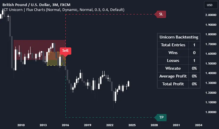
ICT Unicorn | Flux Charts💎 GENERAL OVERVIEW
Introducing our new ICT Unicorn Indicator! This indicator is built around the ICT's "Unicorn" strategy. The strategy uses Breaker Blocks and Fair Value Gaps for entry confirmation. For more information about the process, check the "HOW DOES IT WORK" section.
Features of the new ICT Unicorn Indicator :
Implementation of ICT's Unicorn Strategy
Toggleable Retracement Entry Method
3 Different TP / SL Methods
Customizable Execution Settings
Customizable Backtesting Dashboard
Alerts for Buy, Sell, TP & SL Signals
📌 HOW DOES IT WORK ?
The ICT Unicorn entry model merges the concepts of Breaker Blocks and Fair Value Gaps (FVGs), offering a distinct method for identifying trade opportunities. By integrating these two elements, we can have a position entry with stop-loss and take-profit targets on the potential support & resistance zones. This model is particularly reliable for trade entry, as it combines two powerful entry techniques.
An ICT Unicorn Model consists of a FVG which is overlapping with a Breaker Block of the same type. Here is an example :
When a FVG overlaps with a Breaker Block of the same type, the indicator gives a Buy or Sell signal depending on the FVG type (Bullish & Bearish). If the "Require Retracement" option is enabled in the settings, the signals are not given immediately. Instead, the current price of the ticker will need to touch the FVG once more before the signals are given.
After the Buy or Sell signal, the indicator immediately draws the take-profit (TP) and stop-loss (SL) targets. The indicator has three different TP & SL modes, explained in the "Settings" section of this write-up.
You can set up alerts for entry and TP & SL signals, and also check the current performance of the indicator and adjust the settings accordingly to the current ticker using the backtesting dashboard.
🚩 UNIQUENESS
This indicator is an all-in-one suit for the ICT's Unicorn concept. It's capable of plotting the strategy, giving signals, a backtesting dashboard and alerts feature. Different and customizable algorithm modes will help the trader fine-tune the indicator for the asset they are currently trading. Three different TP / SL modes are available to suit your needs. The backtesting dashboard allows you to see how your settings perform in the current ticker. You can also set up alerts to get informed when the strategy is executable for different tickers.
⚙️ SETTINGS
1. General Configuration
FVG Detection Sensitivity -> You may select between Low, Normal, High or Extreme FVG detection sensitivity. This will essentially determine the size of the spotted FVGs, with lower sensitivies resulting in spotting bigger FVGs, and higher sensitivies resulting in spotting all sizes of FVGs.
Swing Length -> Swing length is used when finding order block formations. Smaller values will result in finding smaller order & breaker blocks.
Require Retracement ->
a) Disabled : The entry signal is given immediately once a FVG overlaps with a Breaker Block of the same type.
b) Enabled : The current price of the ticker will need to touch the FVG once more before the entry signal is given.
2. TP / SL
TP / SL Method ->
a) Unicorn : This is the default option. The SL will be set to the lowest low of the last 100 bars with an extra offset in a Buy signal. For Sell signals, the SL will be set to the highest high of the last 100 bars with an extra offset. The TP is then set to a value using the SL value and maintaining a risk-reward ratio.
b) Dynamic: The TP / SL zones will be auto-determined by the algorithm based on the Average True Range (ATR) of the current ticker.
c) Fixed : You can adjust the exact TP / SL ratios from the settings below.
Dynamic Risk -> The risk you're willing to take if "Dynamic" TP / SL Method is selected. Higher risk usually means a better winrate at the cost of losing more if the strategy fails. This setting is has a crucial effect on the performance of the indicator, as different tickers may have different volatility so the indicator may have increased performance when this setting is correctly adjusted.
PVT Crossover Strategy**Release Notes**
**Strategy Name**: PVT Crossover Strategy
**Purpose**: This strategy aims to capture entry and exit points in the market using the Price-Volume Trend (PVT) and its Exponential Moving Average (EMA). It specifically uses the crossover of PVT with its EMA as signals to identify changes in market trends.
**Uniqueness and Usefulness**
**Uniqueness**: This strategy is unique in its use of the PVT indicator, which combines price changes with trading volume to track trends. The filtering with EMA reduces noise and provides more accurate signals compared to other indicators.
**Usefulness**: This strategy is effective for traders looking to detect trend changes early. The signals based on PVT and its EMA crossover work particularly well in markets where volume fluctuations are significant.
**Entry Conditions**
**Long Entry**:
- **Condition**: A crossover occurs where PVT crosses above its EMA.
- **Signal**: A buy signal is generated, indicating a potential uptrend.
**Short Entry**:
- **Condition**: A crossunder occurs where PVT crosses below its EMA.
- **Signal**: A sell signal is generated, indicating a potential downtrend.
**Exit Conditions**
**Exit Strategy**:
- The strategy does not explicitly program exit conditions beyond the entry signals, but traders are encouraged to close positions manually based on signals or apply their own risk management strategy.
**Risk Management**
This strategy does not include default risk management rules, so traders should implement their own. Consider using trailing stops or fixed stop losses to manage risk.
**Account Size**: ¥100,000
**Commissions and Slippage**: 94 pips per trade for commissions and 1 pip for slippage
**Risk per Trade**: 10% of account equity
**Configurable Options**
**Configurable Options**:
- **EMA Length**: The length of the EMA used to calculate the EMA of PVT (default is 20).
- **Signal Display Control**: The option to turn the display of signals on or off.
**Adequate Sample Size**
To ensure the robustness and reliability of this strategy, it is recommended to backtest it with a sufficiently long period of historical data, especially across different market conditions.
**Credits**
**Acknowledgments**:
This strategy is based on the concept of the PVT indicator and its application in strategy design, drawing on contributions from technical analysis and the trading community.
**Clean Chart Description**
**Chart Appearance**:
This strategy is designed to maintain a clean and simple chart by turning off the plot of PVT, its EMA, and entry signals. This reduces clutter and allows for more effective trend analysis.
**Addressing the House Rule Violations**
**Omissions and Unrealistic Claims**
**Clarification**:
This strategy does not make unrealistic or unsupported claims about its performance, and all signals are for educational purposes only, not guaranteeing future results. It is important to understand that past performance does not guarantee future outcomes.
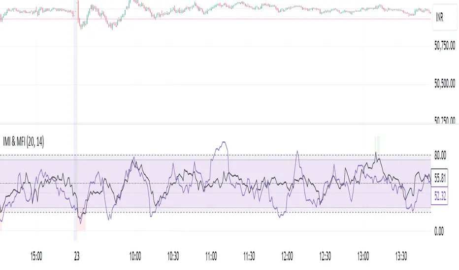
IMI and MFI CombinedFor a strategy using the combined IMI (Intraday Momentum Index), MFI (Money Flow Index), and Bollinger Bands on a 1-minute chart of Bank NIFTY (Bank Nifty Index), here's how you can interpret the indicators and define a sell signal strategy:
Strategy Explanation:
IMI (Intraday Momentum Index):
IMI measures the ratio of upward price changes to downward price changes over a specified period, indicating momentum.
In the script, IMI is plotted with a range from 0 to 100. Levels above 75 are considered overbought, and levels below 25 are oversold.
Strategy Condition: A sell signal can be considered when IMI is above 75, indicating a potentially overbought market condition.
MFI (Money Flow Index):
MFI measures the strength of money flowing in and out of a security, using price and volume.
In the script, MFI is plotted with levels at 80 (overbought) and 20 (oversold).
Strategy Condition: A sell signal can be considered when MFI is above 80, suggesting an overbought condition in the market.
Bollinger Bands:
Bollinger Bands consist of a middle band (SMA) and upper/lower bands representing volatility levels around the price.
In the script, Bollinger Bands are plotted with a length of 20 and a standard deviation multiplier of 2.
Strategy Condition: While not explicitly used for generating sell signals in this script, Bollinger Bands can help confirm price volatility and potential reversals when combined with other indicators.
Sell Signal Criteria:
IMI Sell Signal: Look for instances where IMI rises above 75. This indicates that the recent upward price momentum may be reaching an unsustainable level, potentially signaling a reversal or a pullback in prices.
MFI Sell Signal: Look for MFI rising above 80. This suggests that the market has experienced strong buying pressure, possibly leading to an overbought condition where a price correction or reversal might occur.
Implementation Considerations:
Confirmation: Consider waiting for both IMI and MFI to confirm the overbought condition simultaneously before entering a sell trade. This can increase the reliability of the signal.
Risk Management: Use stop-loss orders to manage risk in case the market moves against the anticipated direction after the sell signal is triggered.
Timeframe: This strategy is tailored for a 1-minute chart, meaning signals should be interpreted and acted upon quickly due to the rapid nature of price movements in intraday trading.
By combining these indicators and interpreting their signals, you can develop a systematic approach to identifying potential sell opportunities in the Bank NIFTY index on a 1-minute timeframe. Adjustments to indicator parameters and additional technical analysis may further refine the strategy based on your trading preferences and risk tolerance.
Enhanced BOS Strategy with SL/TP and EMA TableDescription:
The Enhanced BOS (Break of Structure) Strategy is an advanced open-source trading indicator designed to identify key market structure changes, integrated with dynamic Stop Loss (SL) and Take Profit (TP) levels, along with an informative EMA (Exponential Moving Average) table for added trend analysis.
Key Features:
Break of Structure (BOS) Detection:
The script detects bullish and bearish BOS by identifying pivot points using a custom pivot period. When the price crosses above or below these points, it signals a potential market trend reversal or continuation.
Dynamic SL/TP Levels:
Users can toggle static SL/TP settings, which automatically calculate levels based on user-defined points. These levels are visualized on the chart with dotted lines and labeled for clarity.
Volume Filters:
The strategy includes a volume condition filter to ensure that only trades within a specified volume range are considered. This helps in avoiding low-volume trades that might lead to false signals.
EMA Table Display:
An on-chart table displaying the current values of the 13-period, 50-period, and 200-period EMAs. This provides a quick reference for trend identification and confirmation, helping traders to stay aligned with the broader market trend.
How It Works:
The script utilizes a combination of moving averages and pivot points to identify potential breakouts or breakdowns in market structure. When a bullish BOS is detected, and the volume conditions are met, the strategy suggests a long position, marking potential SL/TP levels. Similarly, it suggests short positions for bearish BOS.
The EMA table serves as a visual aid, providing real-time updates of the EMA values, allowing traders to gauge the market’s directional bias quickly.
How to Use:
Setting Parameters:
Adjust the pivot period to fine-tune BOS detection according to your trading style and the asset’s volatility.
Configure the SL/TP settings based on your risk tolerance and target profit levels.
Interpreting Signals:
A “Buy” label on the chart indicates a bullish BOS with volume confirmation, signaling a potential long entry.
A “Sell” label indicates a bearish BOS with volume confirmation, signaling a potential short entry.
The EMA table aids in confirming these signals, where the position of the fast, mid, and slow EMAs can provide additional context to the trend’s strength and direction.
Volume Filtering:
Ensure your trades are filtered through the script’s volume condition, which allows for the exclusion of low-volume periods that might generate unreliable signals.
Unique Value:
Unlike many other BOS strategies, this script integrates volume conditions and a visual EMA table, providing a comprehensive toolkit for traders looking to capture market structure shifts while maintaining an eye on trend direction and trade execution precision.
Additional Information:
This script is designed for use on standard bar or candlestick charts for best results.
It is open-source and free to use, encouraging collaboration and improvement by the TradingView community.
By combining powerful trend-following EMAs with the precision of BOS detection and the safety of volume filtering, the Enhanced BOS Strategy offers a balanced approach to trading market structure changes.

RSI with Bollinger Bands Scalp Startegy (1min)
------------------------------------------------------------------------------
The "RSI with Bollinger Bands Scalp Strategy (1min)" is a highly effective tool designed for traders who engage in short-term scalping on the 1-minute chart. This indicator combines the strengths of the RSI (Relative Strength Index) and Bollinger Bands to generate precise buy signals, helping traders make quick and informed decisions in fast-moving markets.
How It Works:
RSI (Relative Strength Index):
The RSI is a widely-used momentum oscillator that measures the speed and change of price movements. It operates on a scale of 0 to 100 and helps identify overbought and oversold conditions in the market.
This strategy allows customization of the RSI's lower and upper bands (default settings: 30 for the lower band and 70 for the upper band) and the RSI length (default: 14).
Bollinger Bands:
Bollinger Bands consist of a central moving average (the basis) and two bands that represent standard deviations above and below the basis. These bands expand and contract based on market volatility.
In this strategy, the Bollinger Bands are used to identify potential buy and sell signals based on the price's relationship to the upper and lower bands.
Signal Generation:
Buy Signal: A buy signal is triggered when two conditions are met:
The RSI value falls below the specified lower band, indicating an oversold condition.
The price crosses below the lower Bollinger Band.
The buy signal is then issued on the first positive candle (where the closing price is greater than or equal to the opening price) after these conditions are met.
Sell Signal: In this version of the strategy, the sell signal is currently disabled to focus solely on generating and optimizing the buy signals for scalping.
Strategy Highlights:
This indicator is particularly effective for traders who focus on 1-minute charts and want to capitalize on rapid price movements.
The combination of RSI and Bollinger Bands ensures that buy signals are only generated during significant oversold conditions, helping to filter out false signals.
Customization:
Users can adjust the RSI length, Bollinger Bands length, and the standard deviation multiplier to better fit their specific trading style and the asset they are trading.
The moving average type for Bollinger Bands can be selected from various options, including SMA, EMA, SMMA, WMA, and VWMA, allowing further customization based on individual preferences.
Usage:
Use this indicator on a 1-minute chart to identify potential buy opportunities during short-term price dips.
Since the sell signals are disabled, this strategy is best used in conjunction with other indicators or strategies to manage exit points effectively.
This "RSI with Bollinger Bands Scalp Strategy (1min)" indicator is a valuable tool for traders looking to enhance their short-term trading performance by focusing on high-probability entry points in volatile market conditions.
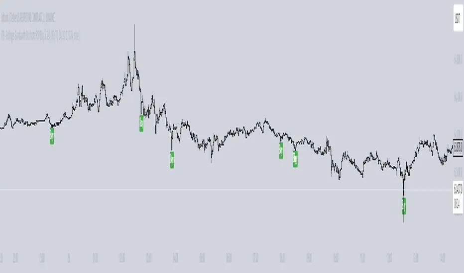
Economic Policy Uncertainty StrategyThis Pine Script strategy is designed to make trading decisions based on the Economic Policy Uncertainty Index for the United States (USEPUINDXD) using a Simple Moving Average (SMA) and a dynamic threshold. The strategy identifies opportunities by entering long positions when the SMA of the Economic Policy Uncertainty Index crosses above a user-defined threshold. An exit is triggered after a set number of bars have passed since the trade was opened. Additionally, the background is highlighted in green when a position is open to visually indicate active trades.
This strategy is intended to be used in portfolio management and trading systems where economic policy uncertainty plays a critical role in decision-making. The index provides insight into macroeconomic conditions, which can affect asset prices and investment returns.
The Economic Policy Uncertainty (EPU) Index is a significant metric used to gauge uncertainty related to economic policies in the United States. This index reflects the frequency of newspaper articles discussing economic uncertainty, government policies, and their potential impact on the economy. It has become a popular indicator for both academics and practitioners to analyze the effects of policy uncertainty on various economic and financial outcomes.
Importance of the EPU Index for Portfolio Decisions:
Economic Policy Uncertainty and Investment Decisions:
Research by Baker, Bloom, and Davis (2016) introduced the Economic Policy Uncertainty Index and explored how increased uncertainty leads to delays in investment and hiring decisions. Their study shows that heightened uncertainty, as captured by the EPU index, is associated with a contraction in economic activity and lower stock market returns. Investors tend to shift their portfolios towards safer assets during periods of high policy uncertainty .
Impact on Asset Prices:
Gulen and Ion (2016) demonstrated that policy uncertainty adversely affects corporate investment, leading to lower stock market returns. The study emphasized that firms reduce investment during periods of high policy uncertainty, which can significantly impact the pricing of risky assets. Consequently, portfolio managers need to account for policy uncertainty when making asset allocation decisions .
Global Implications:
Policy uncertainty is not only a domestic issue. Brogaard and Detzel (2015) found that U.S. economic policy uncertainty has significant spillover effects on global financial markets, affecting equity returns, bond yields, and foreign exchange rates. This suggests that global investors should incorporate U.S. policy uncertainty into their risk management strategies .
These studies underscore the importance of the Economic Policy Uncertainty Index as a tool for understanding macroeconomic risks and making informed portfolio management decisions. Strategies that incorporate the EPU index, such as the one described above, can help investors navigate periods of uncertainty by adjusting their exposure to different asset classes based on economic conditions.