S&R ZonesThis indicator automatically detects swing highs and swing lows on the chart using a 3-bar swing structure. Once a swing point is confirmed, it evaluates the price movement and body size of subsequent candles. If the movement meets a volume-based range condition (2.5× the average body size of the last 5 candles), the indicator creates a zone around that swing.
Swing High Zones: Drawn from the highest price of the swing cluster down to its midpoint.
Swing Low Zones: Drawn from the lowest price of the swing cluster up to its midpoint.
These zones act as dynamic support and resistance levels and remain on the chart until they are either:
Broken (price closes beyond the zone), or
Expired (more than 200 bars old).
Zones are color-coded for clarity:
🔴 Red shaded areas = Swing High resistance zones.
🟢 Green shaded areas = Swing Low support zones.
This makes the indicator useful for identifying high-probability reversal areas, liquidity zones, and supply/demand imbalances that persist until invalidated.
"swing" için komut dosyalarını ara
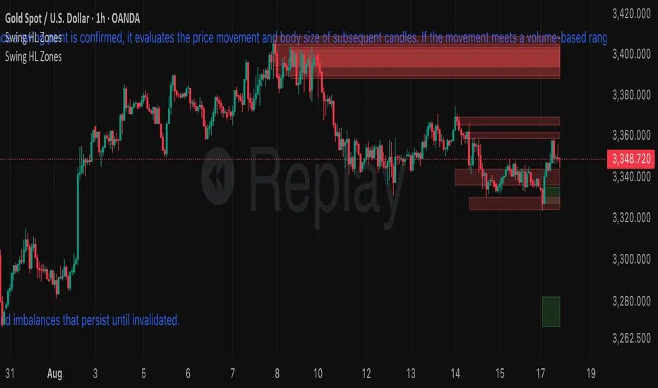
Ayman Entry Signal – Ultimate PRO (Scalping Gold Settings)1. Overview
This indicator is a professional gold scalping tool built for TradingView using Pine Script v6.
It combines multiple price action and technical filters to generate high-probability Buy/Sell signals with built-in trade management features (TP1, TP2, SL, Break Even, Partial Close, Stats tracking).
It is optimized for XAUUSD but can be applied to other assets with proper setting adjustments.
2. Key Features
Multi-Condition Trade Signals – EMA trend, Break of Structure, Order Blocks, FVG, Liquidity Sweeps, Pin Bars, Higher Timeframe confirmation, Trend Cloud, SMA Cross, and ADX.
Full Trade Management – Auto-calculates lot size, SL, TP1, TP2, Break Even, Partial Close.
Dynamic Chart Drawing – Entry lines, SL/TP lines, trade boxes, and real-time PnL.
Statistics Panel – Tracks wins, losses, breakeven trades, and total PnL over selected dates.
Customizable Filters – All filters can be turned ON/OFF to match your strategy.
3. Main Inputs & Settings
Account Settings
Capital ($) – Total trading capital.
Risk Percentage (%) – Risk per trade.
TP to SL Ratio – Risk-to-reward ratio.
Value Per Point ($) – Value per pip/point for lot size calculation.
SL Buffer – Extra points added to SL to avoid stop hunts.
Take Profit Settings
TP1 % of Full Target – Fraction of TP1 compared to TP2.
Move SL to Entry after TP1? – Activates Break Even after TP1.
Break Even Buffer – Extra points when moving SL to BE.
Take Partial Close at TP1 – Option to close half at TP1.
Signal Filters
ATR Period – For SL/TP calculation buffer.
EMA Trend – Uses EMA 9/21 crossover for trend.
Break of Structure (BoS) – Requires structure break confirmation.
Order Block (OB) – Validates trades within OB zones.
Fair Value Gap (FVG) – Confirms trades inside FVGs.
Liquidity Sweep – Checks if liquidity zones are swept.
Pin Bar Confirmation – Uses candlestick patterns for extra confirmation.
Pin Bar Body Ratio – Controls strictness of Pin Bar filter.
Higher Timeframe Filters (HTF)
HTF EMA Confirmation – Confirms lower timeframe trades with higher timeframe trend.
HTF BoS – Confirms with higher timeframe structure break.
HTF Timeframe – Selects higher timeframe.
Advanced Filters
SuperTrend Filter – Confirms trades based on SuperTrend.
ADX Filter – Filters out low volatility periods.
SMA Cross Filter – Uses SMA 8/9 cross as filter.
Trend Cloud Filter – Uses EMA 50/200 as a cloud trend filter.
4. How It Works
Buy Signal Conditions
EMA 9 > EMA 21 (trend bullish)
Optional filters (BoS, OB, FVG, Liquidity Sweep, Pin Bar, HTF confirmations, ADX, SMA Cross, Trend Cloud) must pass if enabled.
When all active filters pass → Buy signal triggers.
Sell Signal Conditions
EMA 9 < EMA 21 (trend bearish)
Same filtering process but for bearish conditions.
When all active filters pass → Sell signal triggers.
5. Trade Execution & Management
When a signal triggers:
Lot size is auto-calculated based on risk % and SL distance.
SL is placed beyond recent swing high/low + ATR buffer.
TP1 and TP2 are calculated from the SL using the reward-to-risk ratio.
Break Even: If enabled, SL moves to entry price after TP1 is hit.
Partial Close: If enabled, half of the position closes at TP1.
Trade Exit: Full exit at TP2, SL hit, or partial close at TP1.
6. Chart Display
Entry Line – Shows entry price.
SL Line – Red dashed line at stop loss level.
TP1 Line – Lime dashed line for TP1.
TP2 Line – Green dashed line for TP2.
PnL Labels – Displays real-time profit/loss in $.
Trade Box – Visual area showing trade range.
Pin Bar Shapes – Optional, marks Pin Bars.
7. Statistics Panel
Stats Header – Shows “Stats”.
Total Trades
Wins
Losses
Breakeven Trades
Total PnL
Can be reset or filtered by date.
8. How to Use
Load the Indicator in TradingView.
Select Gold (XAUUSD) on your preferred scalping timeframe (1m, 5m, 15m).
Adjust settings:
Use default gold scalping settings for quick start.
Enable/disable filters according to your style.
Wait for a Buy/Sell alert.
Confirm visually that all desired conditions align.
Place trade with calculated lot size, SL, and TP levels shown on chart.
Let trade run – the indicator manages Break Even & Partial Close if enabled.
9. Recommended Timeframes
Scalping: 1m, 5m, 15m
Day Trading: 15m, 30m, 1H
Swing: 4H, Daily (adjust settings accordingly)
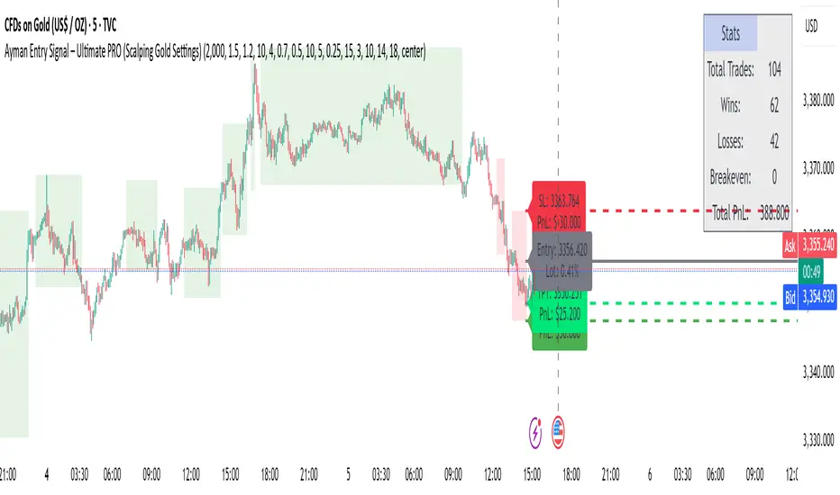
FEDFUNDS Rate Divergence Oscillator [BackQuant]FEDFUNDS Rate Divergence Oscillator
1. Concept and Rationale
The United States Federal Funds Rate is the anchor around which global dollar liquidity and risk-free yield expectations revolve. When the Fed hikes, borrowing costs rise, liquidity tightens and most risk assets encounter head-winds. When it cuts, liquidity expands, speculative appetite often recovers. Bitcoin, a 24-hour permissionless asset sometimes described as “digital gold with venture-capital-like convexity,” is particularly sensitive to macro-liquidity swings.
The FED Divergence Oscillator quantifies the behavioural gap between short-term monetary policy (proxied by the effective Fed Funds Rate) and Bitcoin’s own percentage price change. By converting each series into identical rate-of-change units, subtracting them, then optionally smoothing the result, the script produces a single bounded-yet-dynamic line that tells you, at a glance, whether Bitcoin is outperforming or underperforming the policy backdrop—and by how much.
2. Data Pipeline
• Fed Funds Rate – Pulled directly from the FRED database via the ticker “FRED:FEDFUNDS,” sampled at daily frequency to synchronise with crypto closes.
• Bitcoin Price – By default the script forces a daily timeframe so that both series share time alignment, although you can disable that and plot the oscillator on intraday charts if you prefer.
• User Source Flexibility – The BTC series is not hard-wired; you can select any exchange-specific symbol or even swap BTC for another crypto or risk asset whose interaction with the Fed rate you wish to study.
3. Math under the Hood
(1) Rate of Change (ROC) – Both the Fed rate and BTC close are converted to percent return over a user-chosen lookback (default 30 bars). This means a cut from 5.25 percent to 5.00 percent feeds in as –4.76 percent, while a climb from 25 000 to 30 000 USD in BTC over the same window converts to +20 percent.
(2) Divergence Construction – The script subtracts the Fed ROC from the BTC ROC. Positive values show BTC appreciating faster than policy is tightening (or falling slower than the rate is cutting); negative values show the opposite.
(3) Optional Smoothing – Macro series are noisy. Toggle “Apply Smoothing” to calm the line with your preferred moving-average flavour: SMA, EMA, DEMA, TEMA, RMA, WMA or Hull. The default EMA-25 removes day-to-day whips while keeping turning points alive.
(4) Dynamic Colour Mapping – Rather than using a single hue, the oscillator line employs a gradient where deep greens represent strong bullish divergence and dark reds flag sharp bearish divergence. This heat-map approach lets you gauge intensity without squinting at numbers.
(5) Threshold Grid – Five horizontal guides create a structured regime map:
• Lower Extreme (–50 pct) and Upper Extreme (+50 pct) identify panic capitulations and euphoria blow-offs.
• Oversold (–20 pct) and Overbought (+20 pct) act as early warning alarms.
• Zero Line demarcates neutral alignment.
4. Chart Furniture and User Interface
• Oscillator fill with a secondary DEMA-30 “shader” offers depth perception: fat ribbons often precede high-volatility macro shifts.
• Optional bar-colouring paints candles green when the oscillator is above zero and red below, handy for visual correlation.
• Background tints when the line breaches extreme zones, making macro inflection weeks pop out in the replay bar.
• Everything—line width, thresholds, colours—can be customised so the indicator blends into any template.
5. Interpretation Guide
Macro Liquidity Pulse
• When the oscillator spends weeks above +20 while the Fed is still raising rates, Bitcoin is signalling liquidity tolerance or an anticipatory pivot view. That condition often marks the embryonic phase of major bull cycles (e.g., March 2020 rebound).
• Sustained prints below –20 while the Fed is already dovish indicate risk aversion or idiosyncratic crypto stress—think exchange scandals or broad flight to safety.
Regime Transition Signals
• Bullish cross through zero after a long sub-zero stint shows Bitcoin regaining upward escape velocity versus policy.
• Bearish cross under zero during a hiking cycle tells you monetary tightening has finally started to bite.
Momentum Exhaustion and Mean-Reversion
• Touches of +50 (or –50) come rarely; they are statistically stretched events. Fade strategies either taking profits or hedging have historically enjoyed positive expectancy.
• Inside-bar candlestick patterns or lower-timeframe bearish engulfings simultaneously with an extreme overbought print make high-probability short scalp setups, especially near weekly resistance. The same logic mirrors for oversold.
Pair Trading / Relative Value
• Combine the oscillator with spreads like BTC versus Nasdaq 100. When both the FED Divergence oscillator and the BTC–NDQ relative-strength line roll south together, the cross-asset confirmation amplifies conviction in a mean-reversion short.
• Swap BTC for miners, altcoins or high-beta equities to test who is the divergence leader.
Event-Driven Tactics
• FOMC days: plot the oscillator on an hourly chart (disable ‘Force Daily TF’). Watch for micro-structural spikes that resolve in the first hour after the statement; rapid flips across zero can front-run post-FOMC swings.
• CPI and NFP prints: extremes reached into the release often mean positioning is one-sided. A reversion toward neutral in the first 24 hours is common.
6. Alerts Suite
Pre-bundled conditions let you automate workflows:
• Bullish / Bearish zero crosses – queue spot or futures entries.
• Standard OB / OS – notify for first contact with actionable zones.
• Extreme OB / OS – prime time to review hedges, take profits or build contrarian swing positions.
7. Parameter Playground
• Shorten ROC Lookback to 14 for tactical traders; lengthen to 90 for macro investors.
• Raise extreme thresholds (for example ±80) when plotting on altcoins that exhibit higher volatility than BTC.
• Try HMA smoothing for responsive yet smooth curves on intraday charts.
• Colour-blind users can easily swap bull and bear palette selections for preferred contrasts.
8. Limitations and Best Practices
• The Fed Funds series is step-wise; it only changes on meeting days. Rapid BTC oscillations in between may dominate the calculation. Keep that perspective when interpreting very high-frequency signals.
• Divergence does not equal causation. Crypto-native catalysts (ETF approvals, hack headlines) can overwhelm macro links temporarily.
• Use in conjunction with classical confirmation tools—order-flow footprints, market-profile ledges, or simple price action to avoid “pure-indicator” traps.
9. Final Thoughts
The FEDFUNDS Rate Divergence Oscillator distills an entire macro narrative monetary policy versus risk sentiment into a single colourful heartbeat. It will not magically predict every pivot, yet it excels at framing market context, spotting stretches and timing regime changes. Treat it as a strategic compass rather than a tactical sniper scope, combine it with sound risk management and multi-factor confirmation, and you will possess a robust edge anchored in the world’s most influential interest-rate benchmark.
Trade consciously, stay adaptive, and let the policy-price tension guide your roadmap.
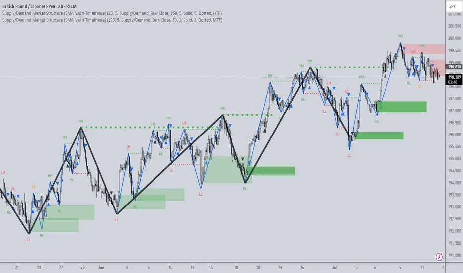
Supply/Demand Market Structure (SMA Multi-Timeframe)Supply/Demand Based Market Structure
Structure + Order Blocks from Synthetic SMA Candles
Overview:
The SMA Supply/Demand Market Structure indicator combines market structure analysis with supply/demand logic, powered by SMA-based synthetic candles . Instead of relying on raw candle data, this tool generates smoothed higher-timeframe candles using simple moving averages to identify more stable zones and cleaner structure shifts.
It detects bullish and bearish breaks of structure (BoS) , highlights swing points like HH, HL, LH, LL , and plots institutional-style supply and demand zones formed from aggressive rallies or drops. The result is a precise and noise-filtered view of market intent, perfect for trend-following or smart money strategies.
How It Works:
- Synthetic candles are created using SMA of OHLC values on your selected timeframe (HTF).
- A bullish break occurs when price closes above the high of the last bearish synthetic candle.
- A bearish break occurs when price closes below the low of the last bullish synthetic candle.
- Upon break confirmation:
- A demand zone is drawn using the last bearish candle.
- A supply zone is drawn using the last bullish candle.
- Each zone is extended forward for a user-defined number of bars and optionally deleted upon mitigation.
- Zigzag-based internal structure connects valid swing points and classifies them as HH, HL, LH, LL , including Liquidity Sweeps (LS) .
- BoS levels are highlighted with lines that automatically reset when new structure forms.
Key Features:
- Synthetic SMA Candles : Smooth and reliable structure from average-based HTF candles
- Break Modes : Choose between raw HTF closes or SMA closes for break logic
- Custom Timeframe Selection : Analyze structure across any HTF you choose
- Dynamic Supply/Demand Zones : Auto-plot boxes from valid rallies/drops
- Mitigation Detection : Optionally fade or delete zones when price trades through
- Zigzag Structure Mapping : Automatically connect structural highs/lows
- BoS Detection : Real-time breakout of swing points with visual confirmation
- Smart Labels : Marks HH, HL, LH, LL, and LS directly on the chart
- Multi-timeframe Alert System : Notify for all structural changes, BoS, and new zones
How to Use:
- Set your desired HTF and SMA Length for synthetic candle smoothing.
- Use SMA=1 for raw candles
- Select a Break Mode :
- Raw Close : Uses standard HTF close values
- SMA Close : Uses smoothed closes from SMA
- Watch for bullish or bearish breaks — zones are plotted when price confirms breakout structure.
- Use demand zones as long entry areas and supply zones as short setups on retests.
- Rely on internal shifts and zigzag swings to monitor structure continuity.
- Enable alerts for swing formations, BoS, and liquidity sweeps to trade hands-free.
Recommended Strategies:
- Smart Money & ICT Models : Use synthetic demand/supply + BoS for mitigation or continuation plays
- Swing Trading : Align with higher timeframe structure and use zones for entry triggers
- Trend Trading : Confirm structure alignment and wait for pullbacks into zones
- Reversal Entries : Trade structure breaks when zones fail and a BoS confirms the shift
Customization Options:
- Timeframe input for custom HTF control
- SMA Length to adjust candle smoothing
- Zone Style : Control zone color, transparency, and duration
- Structure Display : Toggle swing labels and zigzag visuals
- Alert Mode : Choose between LTF, MTF, or HTF alerts
Summary:
SMA Supply/Demand Market Structure provides a clean, flexible view of price structure and institutional intent by fusing market structure with SMA-based synthetic candles. It’s ideal for anyone seeking reduced noise, visually guided entries, and rule-based trading based on structural shifts and real-time demand/supply dynamics.
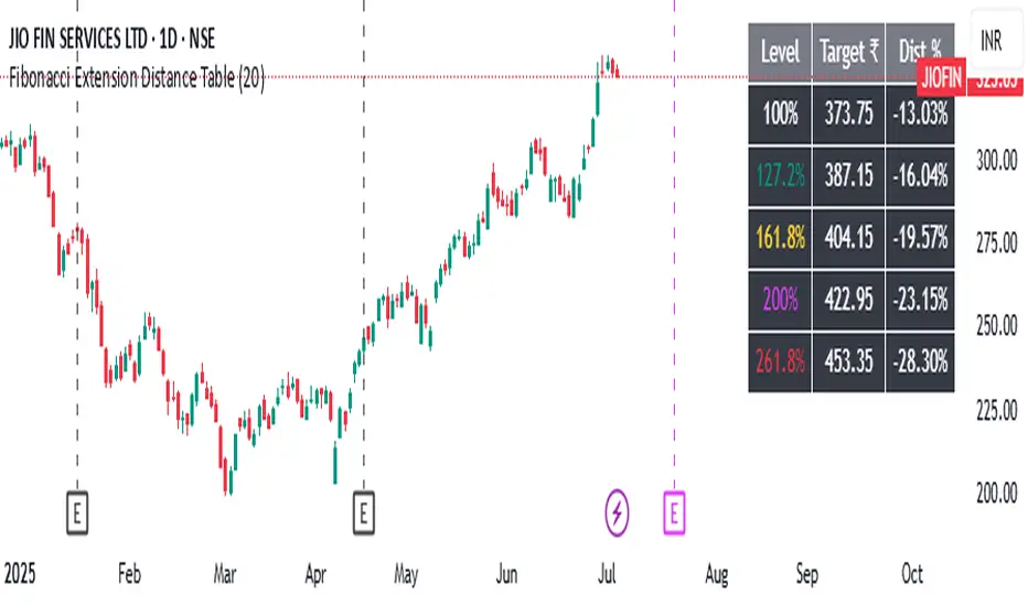
Fibonacci Extension Distance Table## 🧾 **Script Name**: Fibonacci Extension Distance Table
### 🎯 Purpose:
This script helps traders visually track **key Fibonacci extension levels** on any chart and immediately see:
* The **price target** at each extension
* The **distance in percentage** from the current market price
It is especially helpful for:
* **Profit targets in trending trades**
* Monitoring **potential resistance zones** in uptrends
* Planning **entry/exit timing**
---
## 🧮 **How It Works**
1. **Swing Logic (A → B → C)**
* It automatically finds:
* `A`: the **lowest low** in the last `swingLen` bars
* `B`: the **highest high** in that same lookback
* `C`: current bar’s low is used as the **retracement point** (simplified)
2. **Extension Formula**
Using the Fibonacci formula:
```text
Extension Price = C + (B - A) × Fibonacci Ratio
```
The script calculates projected target prices at:
* **100%**
* **127.2%**
* **161.8%** (Golden Ratio)
* **200%**
* **261.8%**
3. **Distance Calculation**
For each level, it calculates:
* The **absolute difference** between current price and the extension level
* The **percentage difference**, which helps quickly assess how close or far the market is from that target
---
## 📋 **Table Output in Top Right**
| Level | Target ₹ | Dist % from current price |
| ------ | ---------- | ------------------------- |
| 100% | Calculated | % Above/Below |
| 127.2% | Calculated | % Above/Below |
| 161.8% | Calculated | % Above/Below |
| 200% | Calculated | % Above/Below |
| 261.8% | Calculated | % Above/Below |
* The table updates **live on each bar**
* It **highlights levels** where price is nearing
* Useful in **any time frame** and **any market** (stocks, crypto, forex)
---
## 🔔 Example Use Case
You bought a stock at ₹100, and recent swing shows:
* A = ₹80
* B = ₹110
* C = ₹100
The 161.8% extension = 100 + (110 − 80) × 1.618 = ₹148.54
If the current price is ₹144, the table will show:
* Golden Ratio Target: ₹148.54
* Distance: −4.54
* Distance %: −3.05%
You now know your **target is near** and can plan your **exit or trailing stop**.
---
## 🧠 Benefits
* No need to draw extensions manually
* Automatically adapts to new swing structures
* Supports **scalping**, **swing**, and **positional** strategies
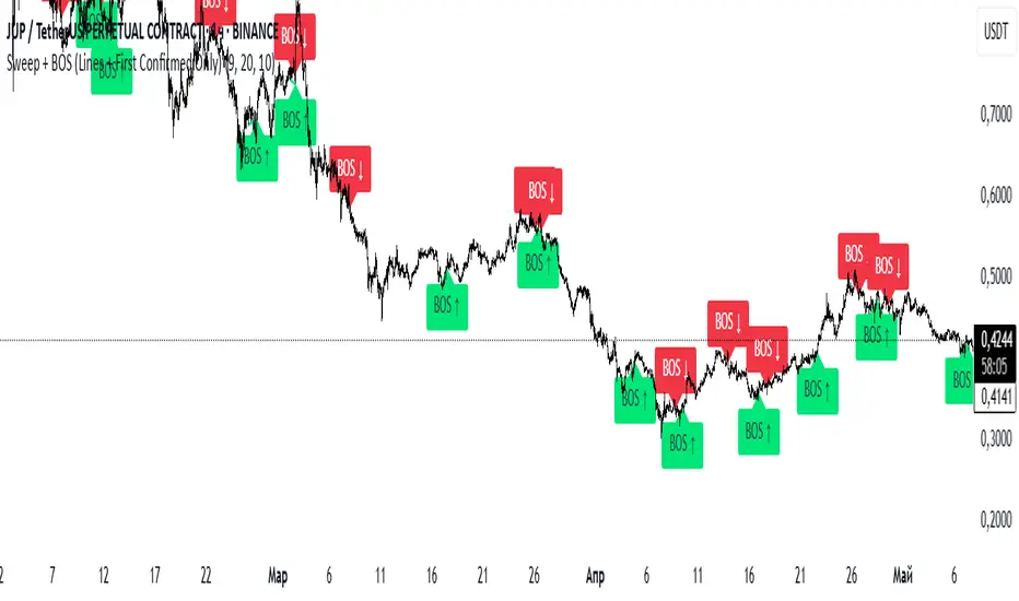
Sweep + BOS (Lines + First Confirmed Only)🔍 Indicator: Sweep + BOS (Break of Structure with Visual Lines)
🧠 Overview
This indicator combines Swing detection, Liquidity Sweeps, and Break of Structure (BOS) logic, with:
Customizable swing length,
BOS signals only after confirmed sweeps,
BOS shown only once per sweep,
Visual labels and connecting lines to highlight structure breaks clearly.
⚙️ Inputs
Swing Length:
Defines how many candles to use to identify a swing high/low. Must be an odd number (e.g., 3, 5, 7...).
Sweep Lookback Window:
Sets how far back the script checks for a sweep (false breakout over a swing).
BOS Validity After Sweep:
Number of bars within which a BOS can be considered valid after a sweep.
Toggle Options:
Show/hide:
Swing Labels
Sweep Labels
BOS Labels
BOS Connecting Lines
📌 Logic Breakdown
✅ Swings
Swing High: A candle’s high is greater than the highs of all N candles on both sides.
Swing Low: A candle’s low is lower than the lows of all N candles on both sides.
💧 Liquidity Sweeps
Sweep High:
Price spikes above a previous Swing High,
Then closes back below it (false breakout).
Sweep Low:
Price drops below a previous Swing Low,
Then closes back above it.
🔁 Break of Structure (BOS)
A BOS is only shown if:
It occurs after a valid sweep (within X bars),
It hasn’t been already plotted for that sweep,
BOS ↑ is only possible after Sweep Low,
BOS ↓ is only possible after Sweep High,
Opposite BOS type resets the last BOS state.
BOS ↑ (Bullish):
Confirmed when price closes above previous Swing High after Sweep Low.
Label appears at the candle low.
A line is drawn from the Swing Low to the BOS candle.
BOS ↓ (Bearish):
Confirmed when price closes below previous Swing Low after Sweep High.
Label appears at the candle high.
A line is drawn from the Swing High to the BOS candle.
Williams Fractals with Buy/Sell Signals🧠 Concept:
This indicator is based on the concept of fractal swing highs and lows, commonly used in Bill Williams’ trading methods. A fractal forms when a candle’s high or low is higher/lower than a set number of candles on both sides. This structure helps identify local market turning points.
⚙️ Inputs:
Fractal Sensitivity (swingSensitivity):
Number of candles required on each side of the central bar to validate a fractal.
For example, if set to 2, a swing high is detected when a bar’s high is higher than the previous 2 bars and the next 2 bars.
✅ Features:
Fractal Detection:
Plots white triangles above swing highs (down fractals).
Plots white triangles below swing lows (up fractals).
Buy/Sell Signals:
Buy Signal: Triggered when the candle closes above the most recent down fractal.
Sell Signal: Triggered when the candle closes below the most recent up fractal.
Signals alternate — a Buy must follow a Sell and vice versa to reduce noise.
Signal Labels:
"BUY" label appears below the candle in green.
"SELL" label appears above the candle in red.
Alerts:
Real-time alerts are available for both Buy and Sell signals via alertcondition().
📌 Use Case:
This indicator can help you:
Detect short-term reversals.
Confirm breakouts or structure shifts.
Time entries with clear logic based on price action.
Tensor Market Analysis Engine (TMAE)# Tensor Market Analysis Engine (TMAE)
## Advanced Multi-Dimensional Mathematical Analysis System
*Where Quantum Mathematics Meets Market Structure*
---
## 🎓 THEORETICAL FOUNDATION
The Tensor Market Analysis Engine represents a revolutionary synthesis of three cutting-edge mathematical frameworks that have never before been combined for comprehensive market analysis. This indicator transcends traditional technical analysis by implementing advanced mathematical concepts from quantum mechanics, information theory, and fractal geometry.
### 🌊 Multi-Dimensional Volatility with Jump Detection
**Hawkes Process Implementation:**
The TMAE employs a sophisticated Hawkes process approximation for detecting self-exciting market jumps. Unlike traditional volatility measures that treat price movements as independent events, the Hawkes process recognizes that market shocks cluster and exhibit memory effects.
**Mathematical Foundation:**
```
Intensity λ(t) = μ + Σ α(t - Tᵢ)
```
Where market jumps at times Tᵢ increase the probability of future jumps through the decay function α, controlled by the Hawkes Decay parameter (0.5-0.99).
**Mahalanobis Distance Calculation:**
The engine calculates volatility jumps using multi-dimensional Mahalanobis distance across up to 5 volatility dimensions:
- **Dimension 1:** Price volatility (standard deviation of returns)
- **Dimension 2:** Volume volatility (normalized volume fluctuations)
- **Dimension 3:** Range volatility (high-low spread variations)
- **Dimension 4:** Correlation volatility (price-volume relationship changes)
- **Dimension 5:** Microstructure volatility (intrabar positioning analysis)
This creates a volatility state vector that captures market behavior impossible to detect with traditional single-dimensional approaches.
### 📐 Hurst Exponent Regime Detection
**Fractal Market Hypothesis Integration:**
The TMAE implements advanced Rescaled Range (R/S) analysis to calculate the Hurst exponent in real-time, providing dynamic regime classification:
- **H > 0.6:** Trending (persistent) markets - momentum strategies optimal
- **H < 0.4:** Mean-reverting (anti-persistent) markets - contrarian strategies optimal
- **H ≈ 0.5:** Random walk markets - breakout strategies preferred
**Adaptive R/S Analysis:**
Unlike static implementations, the TMAE uses adaptive windowing that adjusts to market conditions:
```
H = log(R/S) / log(n)
```
Where R is the range of cumulative deviations and S is the standard deviation over period n.
**Dynamic Regime Classification:**
The system employs hysteresis to prevent regime flipping, requiring sustained Hurst values before regime changes are confirmed. This prevents false signals during transitional periods.
### 🔄 Transfer Entropy Analysis
**Information Flow Quantification:**
Transfer entropy measures the directional flow of information between price and volume, revealing lead-lag relationships that indicate future price movements:
```
TE(X→Y) = Σ p(yₜ₊₁, yₜ, xₜ) log
```
**Causality Detection:**
- **Volume → Price:** Indicates accumulation/distribution phases
- **Price → Volume:** Suggests retail participation or momentum chasing
- **Balanced Flow:** Market equilibrium or transition periods
The system analyzes multiple lag periods (2-20 bars) to capture both immediate and structural information flows.
---
## 🔧 COMPREHENSIVE INPUT SYSTEM
### Core Parameters Group
**Primary Analysis Window (10-100, Default: 50)**
The fundamental lookback period affecting all calculations. Optimization by timeframe:
- **1-5 minute charts:** 20-30 (rapid adaptation to micro-movements)
- **15 minute-1 hour:** 30-50 (balanced responsiveness and stability)
- **4 hour-daily:** 50-100 (smooth signals, reduced noise)
- **Asset-specific:** Cryptocurrency 20-35, Stocks 35-50, Forex 40-60
**Signal Sensitivity (0.1-2.0, Default: 0.7)**
Master control affecting all threshold calculations:
- **Conservative (0.3-0.6):** High-quality signals only, fewer false positives
- **Balanced (0.7-1.0):** Optimal risk-reward ratio for most trading styles
- **Aggressive (1.1-2.0):** Maximum signal frequency, requires careful filtering
**Signal Generation Mode:**
- **Aggressive:** Any component signals (highest frequency)
- **Confluence:** 2+ components agree (balanced approach)
- **Conservative:** All 3 components align (highest quality)
### Volatility Jump Detection Group
**Volatility Dimensions (2-5, Default: 3)**
Determines the mathematical space complexity:
- **2D:** Price + Volume volatility (suitable for clean markets)
- **3D:** + Range volatility (optimal for most conditions)
- **4D:** + Correlation volatility (advanced multi-asset analysis)
- **5D:** + Microstructure volatility (maximum sensitivity)
**Jump Detection Threshold (1.5-4.0σ, Default: 3.0σ)**
Standard deviations required for volatility jump classification:
- **Cryptocurrency:** 2.0-2.5σ (naturally volatile)
- **Stock Indices:** 2.5-3.0σ (moderate volatility)
- **Forex Major Pairs:** 3.0-3.5σ (typically stable)
- **Commodities:** 2.0-3.0σ (varies by commodity)
**Jump Clustering Decay (0.5-0.99, Default: 0.85)**
Hawkes process memory parameter:
- **0.5-0.7:** Fast decay (jumps treated as independent)
- **0.8-0.9:** Moderate clustering (realistic market behavior)
- **0.95-0.99:** Strong clustering (crisis/event-driven markets)
### Hurst Exponent Analysis Group
**Calculation Method Options:**
- **Classic R/S:** Original Rescaled Range (fast, simple)
- **Adaptive R/S:** Dynamic windowing (recommended for trading)
- **DFA:** Detrended Fluctuation Analysis (best for noisy data)
**Trending Threshold (0.55-0.8, Default: 0.60)**
Hurst value defining persistent market behavior:
- **0.55-0.60:** Weak trend persistence
- **0.65-0.70:** Clear trending behavior
- **0.75-0.80:** Strong momentum regimes
**Mean Reversion Threshold (0.2-0.45, Default: 0.40)**
Hurst value defining anti-persistent behavior:
- **0.35-0.45:** Weak mean reversion
- **0.25-0.35:** Clear ranging behavior
- **0.15-0.25:** Strong reversion tendency
### Transfer Entropy Parameters Group
**Information Flow Analysis:**
- **Price-Volume:** Classic flow analysis for accumulation/distribution
- **Price-Volatility:** Risk flow analysis for sentiment shifts
- **Multi-Timeframe:** Cross-timeframe causality detection
**Maximum Lag (2-20, Default: 5)**
Causality detection window:
- **2-5 bars:** Immediate causality (scalping)
- **5-10 bars:** Short-term flow (day trading)
- **10-20 bars:** Structural flow (swing trading)
**Significance Threshold (0.05-0.3, Default: 0.15)**
Minimum entropy for signal generation:
- **0.05-0.10:** Detect subtle information flows
- **0.10-0.20:** Clear causality only
- **0.20-0.30:** Very strong flows only
---
## 🎨 ADVANCED VISUAL SYSTEM
### Tensor Volatility Field Visualization
**Five-Layer Resonance Bands:**
The tensor field creates dynamic support/resistance zones that expand and contract based on mathematical field strength:
- **Core Layer (Purple):** Primary tensor field with highest intensity
- **Layer 2 (Neutral):** Secondary mathematical resonance
- **Layer 3 (Info Blue):** Tertiary harmonic frequencies
- **Layer 4 (Warning Gold):** Outer field boundaries
- **Layer 5 (Success Green):** Maximum field extension
**Field Strength Calculation:**
```
Field Strength = min(3.0, Mahalanobis Distance × Tensor Intensity)
```
The field amplitude adjusts to ATR and mathematical distance, creating dynamic zones that respond to market volatility.
**Radiation Line Network:**
During active tensor states, the system projects directional radiation lines showing field energy distribution:
- **8 Directional Rays:** Complete angular coverage
- **Tapering Segments:** Progressive transparency for natural visual flow
- **Pulse Effects:** Enhanced visualization during volatility jumps
### Dimensional Portal System
**Portal Mathematics:**
Dimensional portals visualize regime transitions using category theory principles:
- **Green Portals (◉):** Trending regime detection (appear below price for support)
- **Red Portals (◎):** Mean-reverting regime (appear above price for resistance)
- **Yellow Portals (○):** Random walk regime (neutral positioning)
**Tensor Trail Effects:**
Each portal generates 8 trailing particles showing mathematical momentum:
- **Large Particles (●):** Strong mathematical signal
- **Medium Particles (◦):** Moderate signal strength
- **Small Particles (·):** Weak signal continuation
- **Micro Particles (˙):** Signal dissipation
### Information Flow Streams
**Particle Stream Visualization:**
Transfer entropy creates flowing particle streams indicating information direction:
- **Upward Streams:** Volume leading price (accumulation phases)
- **Downward Streams:** Price leading volume (distribution phases)
- **Stream Density:** Proportional to information flow strength
**15-Particle Evolution:**
Each stream contains 15 particles with progressive sizing and transparency, creating natural flow visualization that makes information transfer immediately apparent.
### Fractal Matrix Grid System
**Multi-Timeframe Fractal Levels:**
The system calculates and displays fractal highs/lows across five Fibonacci periods:
- **8-Period:** Short-term fractal structure
- **13-Period:** Intermediate-term patterns
- **21-Period:** Primary swing levels
- **34-Period:** Major structural levels
- **55-Period:** Long-term fractal boundaries
**Triple-Layer Visualization:**
Each fractal level uses three-layer rendering:
- **Shadow Layer:** Widest, darkest foundation (width 5)
- **Glow Layer:** Medium white core line (width 3)
- **Tensor Layer:** Dotted mathematical overlay (width 1)
**Intelligent Labeling System:**
Smart spacing prevents label overlap using ATR-based minimum distances. Labels include:
- **Fractal Period:** Time-based identification
- **Topological Class:** Mathematical complexity rating (0, I, II, III)
- **Price Level:** Exact fractal price
- **Mahalanobis Distance:** Current mathematical field strength
- **Hurst Exponent:** Current regime classification
- **Anomaly Indicators:** Visual strength representations (○ ◐ ● ⚡)
### Wick Pressure Analysis
**Rejection Level Mathematics:**
The system analyzes candle wick patterns to project future pressure zones:
- **Upper Wick Analysis:** Identifies selling pressure and resistance zones
- **Lower Wick Analysis:** Identifies buying pressure and support zones
- **Pressure Projection:** Extends lines forward based on mathematical probability
**Multi-Layer Glow Effects:**
Wick pressure lines use progressive transparency (1-8 layers) creating natural glow effects that make pressure zones immediately visible without cluttering the chart.
### Enhanced Regime Background
**Dynamic Intensity Mapping:**
Background colors reflect mathematical regime strength:
- **Deep Transparency (98% alpha):** Subtle regime indication
- **Pulse Intensity:** Based on regime strength calculation
- **Color Coding:** Green (trending), Red (mean-reverting), Neutral (random)
**Smoothing Integration:**
Regime changes incorporate 10-bar smoothing to prevent background flicker while maintaining responsiveness to genuine regime shifts.
### Color Scheme System
**Six Professional Themes:**
- **Dark (Default):** Professional trading environment optimization
- **Light:** High ambient light conditions
- **Classic:** Traditional technical analysis appearance
- **Neon:** High-contrast visibility for active trading
- **Neutral:** Minimal distraction focus
- **Bright:** Maximum visibility for complex setups
Each theme maintains mathematical accuracy while optimizing visual clarity for different trading environments and personal preferences.
---
## 📊 INSTITUTIONAL-GRADE DASHBOARD
### Tensor Field Status Section
**Field Strength Display:**
Real-time Mahalanobis distance calculation with dynamic emoji indicators:
- **⚡ (Lightning):** Extreme field strength (>1.5× threshold)
- **● (Solid Circle):** Strong field activity (>1.0× threshold)
- **○ (Open Circle):** Normal field state
**Signal Quality Rating:**
Democratic algorithm assessment:
- **ELITE:** All 3 components aligned (highest probability)
- **STRONG:** 2 components aligned (good probability)
- **GOOD:** 1 component active (moderate probability)
- **WEAK:** No clear component signals
**Threshold and Anomaly Monitoring:**
- **Threshold Display:** Current mathematical threshold setting
- **Anomaly Level (0-100%):** Combined volatility and volume spike measurement
- **>70%:** High anomaly (red warning)
- **30-70%:** Moderate anomaly (orange caution)
- **<30%:** Normal conditions (green confirmation)
### Tensor State Analysis Section
**Mathematical State Classification:**
- **↑ BULL (Tensor State +1):** Trending regime with bullish bias
- **↓ BEAR (Tensor State -1):** Mean-reverting regime with bearish bias
- **◈ SUPER (Tensor State 0):** Random walk regime (neutral)
**Visual State Gauge:**
Five-circle progression showing tensor field polarity:
- **🟢🟢🟢⚪⚪:** Strong bullish mathematical alignment
- **⚪⚪🟡⚪⚪:** Neutral/transitional state
- **⚪⚪🔴🔴🔴:** Strong bearish mathematical alignment
**Trend Direction and Phase Analysis:**
- **📈 BULL / 📉 BEAR / ➡️ NEUTRAL:** Primary trend classification
- **🌪️ CHAOS:** Extreme information flow (>2.0 flow strength)
- **⚡ ACTIVE:** Strong information flow (1.0-2.0 flow strength)
- **😴 CALM:** Low information flow (<1.0 flow strength)
### Trading Signals Section
**Real-Time Signal Status:**
- **🟢 ACTIVE / ⚪ INACTIVE:** Long signal availability
- **🔴 ACTIVE / ⚪ INACTIVE:** Short signal availability
- **Components (X/3):** Active algorithmic components
- **Mode Display:** Current signal generation mode
**Signal Strength Visualization:**
Color-coded component count:
- **Green:** 3/3 components (maximum confidence)
- **Aqua:** 2/3 components (good confidence)
- **Orange:** 1/3 components (moderate confidence)
- **Gray:** 0/3 components (no signals)
### Performance Metrics Section
**Win Rate Monitoring:**
Estimated win rates based on signal quality with emoji indicators:
- **🔥 (Fire):** ≥60% estimated win rate
- **👍 (Thumbs Up):** 45-59% estimated win rate
- **⚠️ (Warning):** <45% estimated win rate
**Mathematical Metrics:**
- **Hurst Exponent:** Real-time fractal dimension (0.000-1.000)
- **Information Flow:** Volume/price leading indicators
- **📊 VOL:** Volume leading price (accumulation/distribution)
- **💰 PRICE:** Price leading volume (momentum/speculation)
- **➖ NONE:** Balanced information flow
- **Volatility Classification:**
- **🔥 HIGH:** Above 1.5× jump threshold
- **📊 NORM:** Normal volatility range
- **😴 LOW:** Below 0.5× jump threshold
### Market Structure Section (Large Dashboard)
**Regime Classification:**
- **📈 TREND:** Hurst >0.6, momentum strategies optimal
- **🔄 REVERT:** Hurst <0.4, contrarian strategies optimal
- **🎲 RANDOM:** Hurst ≈0.5, breakout strategies preferred
**Mathematical Field Analysis:**
- **Dimensions:** Current volatility space complexity (2D-5D)
- **Hawkes λ (Lambda):** Self-exciting jump intensity (0.00-1.00)
- **Jump Status:** 🚨 JUMP (active) / ✅ NORM (normal)
### Settings Summary Section (Large Dashboard)
**Active Configuration Display:**
- **Sensitivity:** Current master sensitivity setting
- **Lookback:** Primary analysis window
- **Theme:** Active color scheme
- **Method:** Hurst calculation method (Classic R/S, Adaptive R/S, DFA)
**Dashboard Sizing Options:**
- **Small:** Essential metrics only (mobile/small screens)
- **Normal:** Balanced information density (standard desktop)
- **Large:** Maximum detail (multi-monitor setups)
**Position Options:**
- **Top Right:** Standard placement (avoids price action)
- **Top Left:** Wide chart optimization
- **Bottom Right:** Recent price focus (scalping)
- **Bottom Left:** Maximum price visibility (swing trading)
---
## 🎯 SIGNAL GENERATION LOGIC
### Multi-Component Convergence System
**Component Signal Architecture:**
The TMAE generates signals through sophisticated component analysis rather than simple threshold crossing:
**Volatility Component:**
- **Jump Detection:** Mahalanobis distance threshold breach
- **Hawkes Intensity:** Self-exciting process activation (>0.2)
- **Multi-dimensional:** Considers all volatility dimensions simultaneously
**Hurst Regime Component:**
- **Trending Markets:** Price above SMA-20 with positive momentum
- **Mean-Reverting Markets:** Price at Bollinger Band extremes
- **Random Markets:** Bollinger squeeze breakouts with directional confirmation
**Transfer Entropy Component:**
- **Volume Leadership:** Information flow from volume to price
- **Volume Spike:** Volume 110%+ above 20-period average
- **Flow Significance:** Above entropy threshold with directional bias
### Democratic Signal Weighting
**Signal Mode Implementation:**
- **Aggressive Mode:** Any single component triggers signal
- **Confluence Mode:** Minimum 2 components must agree
- **Conservative Mode:** All 3 components must align
**Momentum Confirmation:**
All signals require momentum confirmation:
- **Long Signals:** RSI >50 AND price >EMA-9
- **Short Signals:** RSI <50 AND price 0.6):**
- **Increase Sensitivity:** Catch momentum continuation
- **Lower Mean Reversion Threshold:** Avoid counter-trend signals
- **Emphasize Volume Leadership:** Institutional accumulation/distribution
- **Tensor Field Focus:** Use expansion for trend continuation
- **Signal Mode:** Aggressive or Confluence for trend following
**Range-Bound Markets (Hurst <0.4):**
- **Decrease Sensitivity:** Avoid false breakouts
- **Lower Trending Threshold:** Quick regime recognition
- **Focus on Price Leadership:** Retail sentiment extremes
- **Fractal Grid Emphasis:** Support/resistance trading
- **Signal Mode:** Conservative for high-probability reversals
**Volatile Markets (High Jump Frequency):**
- **Increase Hawkes Decay:** Recognize event clustering
- **Higher Jump Threshold:** Avoid noise signals
- **Maximum Dimensions:** Capture full volatility complexity
- **Reduce Position Sizing:** Risk management adaptation
- **Enhanced Visuals:** Maximum information for rapid decisions
**Low Volatility Markets (Low Jump Frequency):**
- **Decrease Jump Threshold:** Capture subtle movements
- **Lower Hawkes Decay:** Treat moves as independent
- **Reduce Dimensions:** Simplify analysis
- **Increase Position Sizing:** Capitalize on compressed volatility
- **Minimal Visuals:** Reduce distraction in quiet markets
---
## 🚀 ADVANCED TRADING STRATEGIES
### The Mathematical Convergence Method
**Entry Protocol:**
1. **Fractal Grid Approach:** Monitor price approaching significant fractal levels
2. **Tensor Field Confirmation:** Verify field expansion supporting direction
3. **Portal Signal:** Wait for dimensional portal appearance
4. **ELITE/STRONG Quality:** Only trade highest quality mathematical signals
5. **Component Consensus:** Confirm 2+ components agree in Confluence mode
**Example Implementation:**
- Price approaching 21-period fractal high
- Tensor field expanding upward (bullish mathematical alignment)
- Green portal appears below price (trending regime confirmation)
- ELITE quality signal with 3/3 components active
- Enter long position with stop below fractal level
**Risk Management:**
- **Stop Placement:** Below/above fractal level that generated signal
- **Position Sizing:** Based on Mahalanobis distance (higher distance = smaller size)
- **Profit Targets:** Next fractal level or tensor field resistance
### The Regime Transition Strategy
**Regime Change Detection:**
1. **Monitor Hurst Exponent:** Watch for persistent moves above/below thresholds
2. **Portal Color Change:** Regime transitions show different portal colors
3. **Background Intensity:** Increasing regime background intensity
4. **Mathematical Confirmation:** Wait for regime confirmation (hysteresis)
**Trading Implementation:**
- **Trending Transitions:** Trade momentum breakouts, follow trend
- **Mean Reversion Transitions:** Trade range boundaries, fade extremes
- **Random Transitions:** Trade breakouts with tight stops
**Advanced Techniques:**
- **Multi-Timeframe:** Confirm regime on higher timeframe
- **Early Entry:** Enter on regime transition rather than confirmation
- **Regime Strength:** Larger positions during strong regime signals
### The Information Flow Momentum Strategy
**Flow Detection Protocol:**
1. **Monitor Transfer Entropy:** Watch for significant information flow shifts
2. **Volume Leadership:** Strong edge when volume leads price
3. **Flow Acceleration:** Increasing flow strength indicates momentum
4. **Directional Confirmation:** Ensure flow aligns with intended trade direction
**Entry Signals:**
- **Volume → Price Flow:** Enter during accumulation/distribution phases
- **Price → Volume Flow:** Enter on momentum confirmation breaks
- **Flow Reversal:** Counter-trend entries when flow reverses
**Optimization:**
- **Scalping:** Use immediate flow detection (2-5 bar lag)
- **Swing Trading:** Use structural flow (10-20 bar lag)
- **Multi-Asset:** Compare flow between correlated assets
### The Tensor Field Expansion Strategy
**Field Mathematics:**
The tensor field expansion indicates mathematical pressure building in market structure:
**Expansion Phases:**
1. **Compression:** Field contracts, volatility decreases
2. **Tension Building:** Mathematical pressure accumulates
3. **Expansion:** Field expands rapidly with directional movement
4. **Resolution:** Field stabilizes at new equilibrium
**Trading Applications:**
- **Compression Trading:** Prepare for breakout during field contraction
- **Expansion Following:** Trade direction of field expansion
- **Reversion Trading:** Fade extreme field expansion
- **Multi-Dimensional:** Consider all field layers for confirmation
### The Hawkes Process Event Strategy
**Self-Exciting Jump Trading:**
Understanding that market shocks cluster and create follow-on opportunities:
**Jump Sequence Analysis:**
1. **Initial Jump:** First volatility jump detected
2. **Clustering Phase:** Hawkes intensity remains elevated
3. **Follow-On Opportunities:** Additional jumps more likely
4. **Decay Period:** Intensity gradually decreases
**Implementation:**
- **Jump Confirmation:** Wait for mathematical jump confirmation
- **Direction Assessment:** Use other components for direction
- **Clustering Trades:** Trade subsequent moves during high intensity
- **Decay Exit:** Exit positions as Hawkes intensity decays
### The Fractal Confluence System
**Multi-Timeframe Fractal Analysis:**
Combining fractal levels across different periods for high-probability zones:
**Confluence Zones:**
- **Double Confluence:** 2 fractal levels align
- **Triple Confluence:** 3+ fractal levels cluster
- **Mathematical Confirmation:** Tensor field supports the level
- **Information Flow:** Transfer entropy confirms direction
**Trading Protocol:**
1. **Identify Confluence:** Find 2+ fractal levels within 1 ATR
2. **Mathematical Support:** Verify tensor field alignment
3. **Signal Quality:** Wait for STRONG or ELITE signal
4. **Risk Definition:** Use fractal level for stop placement
5. **Profit Targeting:** Next major fractal confluence zone
---
## ⚠️ COMPREHENSIVE RISK MANAGEMENT
### Mathematical Position Sizing
**Mahalanobis Distance Integration:**
Position size should inversely correlate with mathematical field strength:
```
Position Size = Base Size × (Threshold / Mahalanobis Distance)
```
**Risk Scaling Matrix:**
- **Low Field Strength (<2.0):** Standard position sizing
- **Moderate Field Strength (2.0-3.0):** 75% position sizing
- **High Field Strength (3.0-4.0):** 50% position sizing
- **Extreme Field Strength (>4.0):** 25% position sizing or no trade
### Signal Quality Risk Adjustment
**Quality-Based Position Sizing:**
- **ELITE Signals:** 100% of planned position size
- **STRONG Signals:** 75% of planned position size
- **GOOD Signals:** 50% of planned position size
- **WEAK Signals:** No position or paper trading only
**Component Agreement Scaling:**
- **3/3 Components:** Full position size
- **2/3 Components:** 75% position size
- **1/3 Components:** 50% position size or skip trade
### Regime-Adaptive Risk Management
**Trending Market Risk:**
- **Wider Stops:** Allow for trend continuation
- **Trend Following:** Trade with regime direction
- **Higher Position Size:** Trend probability advantage
- **Momentum Stops:** Trail stops based on momentum indicators
**Mean-Reverting Market Risk:**
- **Tighter Stops:** Quick exits on trend continuation
- **Contrarian Positioning:** Trade against extremes
- **Smaller Position Size:** Higher reversal failure rate
- **Level-Based Stops:** Use fractal levels for stops
**Random Market Risk:**
- **Breakout Focus:** Trade only clear breakouts
- **Tight Initial Stops:** Quick exit if breakout fails
- **Reduced Frequency:** Skip marginal setups
- **Range-Based Targets:** Profit targets at range boundaries
### Volatility-Adaptive Risk Controls
**High Volatility Periods:**
- **Reduced Position Size:** Account for wider price swings
- **Wider Stops:** Avoid noise-based exits
- **Lower Frequency:** Skip marginal setups
- **Faster Exits:** Take profits more quickly
**Low Volatility Periods:**
- **Standard Position Size:** Normal risk parameters
- **Tighter Stops:** Take advantage of compressed ranges
- **Higher Frequency:** Trade more setups
- **Extended Targets:** Allow for compressed volatility expansion
### Multi-Timeframe Risk Alignment
**Higher Timeframe Trend:**
- **With Trend:** Standard or increased position size
- **Against Trend:** Reduced position size or skip
- **Neutral Trend:** Standard position size with tight management
**Risk Hierarchy:**
1. **Primary:** Current timeframe signal quality
2. **Secondary:** Higher timeframe trend alignment
3. **Tertiary:** Mathematical field strength
4. **Quaternary:** Market regime classification
---
## 📚 EDUCATIONAL VALUE AND MATHEMATICAL CONCEPTS
### Advanced Mathematical Concepts
**Tensor Analysis in Markets:**
The TMAE introduces traders to tensor analysis, a branch of mathematics typically reserved for physics and advanced engineering. Tensors provide a framework for understanding multi-dimensional market relationships that scalar and vector analysis cannot capture.
**Information Theory Applications:**
Transfer entropy implementation teaches traders about information flow in markets, a concept from information theory that quantifies directional causality between variables. This provides intuition about market microstructure and participant behavior.
**Fractal Geometry in Trading:**
The Hurst exponent calculation exposes traders to fractal geometry concepts, helping understand that markets exhibit self-similar patterns across multiple timeframes. This mathematical insight transforms how traders view market structure.
**Stochastic Process Theory:**
The Hawkes process implementation introduces concepts from stochastic process theory, specifically self-exciting point processes. This provides mathematical framework for understanding why market events cluster and exhibit memory effects.
### Learning Progressive Complexity
**Beginner Mathematical Concepts:**
- **Volatility Dimensions:** Understanding multi-dimensional analysis
- **Regime Classification:** Learning market personality types
- **Signal Democracy:** Algorithmic consensus building
- **Visual Mathematics:** Interpreting mathematical concepts visually
**Intermediate Mathematical Applications:**
- **Mahalanobis Distance:** Statistical distance in multi-dimensional space
- **Rescaled Range Analysis:** Fractal dimension measurement
- **Information Entropy:** Quantifying uncertainty and causality
- **Field Theory:** Understanding mathematical fields in market context
**Advanced Mathematical Integration:**
- **Tensor Field Dynamics:** Multi-dimensional market force analysis
- **Stochastic Self-Excitation:** Event clustering and memory effects
- **Categorical Composition:** Mathematical signal combination theory
- **Topological Market Analysis:** Understanding market shape and connectivity
### Practical Mathematical Intuition
**Developing Market Mathematics Intuition:**
The TMAE serves as a bridge between abstract mathematical concepts and practical trading applications. Traders develop intuitive understanding of:
- **How markets exhibit mathematical structure beneath apparent randomness**
- **Why multi-dimensional analysis reveals patterns invisible to single-variable approaches**
- **How information flows through markets in measurable, predictable ways**
- **Why mathematical models provide probabilistic edges rather than certainties**
---
## 🔬 IMPLEMENTATION AND OPTIMIZATION
### Getting Started Protocol
**Phase 1: Observation (Week 1)**
1. **Apply with defaults:** Use standard settings on your primary trading timeframe
2. **Study visual elements:** Learn to interpret tensor fields, portals, and streams
3. **Monitor dashboard:** Observe how metrics change with market conditions
4. **No trading:** Focus entirely on pattern recognition and understanding
**Phase 2: Pattern Recognition (Week 2-3)**
1. **Identify signal patterns:** Note what market conditions produce different signal qualities
2. **Regime correlation:** Observe how Hurst regimes affect signal performance
3. **Visual confirmation:** Learn to read tensor field expansion and portal signals
4. **Component analysis:** Understand which components drive signals in different markets
**Phase 3: Parameter Optimization (Week 4-5)**
1. **Asset-specific tuning:** Adjust parameters for your specific trading instrument
2. **Timeframe optimization:** Fine-tune for your preferred trading timeframe
3. **Sensitivity adjustment:** Balance signal frequency with quality
4. **Visual customization:** Optimize colors and intensity for your trading environment
**Phase 4: Live Implementation (Week 6+)**
1. **Paper trading:** Test signals with hypothetical trades
2. **Small position sizing:** Begin with minimal risk during learning phase
3. **Performance tracking:** Monitor actual vs. expected signal performance
4. **Continuous optimization:** Refine settings based on real performance data
### Performance Monitoring System
**Signal Quality Tracking:**
- **ELITE Signal Win Rate:** Track highest quality signals separately
- **Component Performance:** Monitor which components provide best signals
- **Regime Performance:** Analyze performance across different market regimes
- **Timeframe Analysis:** Compare performance across different session times
**Mathematical Metric Correlation:**
- **Field Strength vs. Performance:** Higher field strength should correlate with better performance
- **Component Agreement vs. Win Rate:** More component agreement should improve win rates
- **Regime Alignment vs. Success:** Trading with mathematical regime should outperform
### Continuous Optimization Process
**Monthly Review Protocol:**
1. **Performance Analysis:** Review win rates, profit factors, and maximum drawdown
2. **Parameter Assessment:** Evaluate if current settings remain optimal
3. **Market Adaptation:** Adjust for changes in market character or volatility
4. **Component Weighting:** Consider if certain components should receive more/less emphasis
**Quarterly Deep Analysis:**
1. **Mathematical Model Validation:** Verify that mathematical relationships remain valid
2. **Regime Distribution:** Analyze time spent in different market regimes
3. **Signal Evolution:** Track how signal characteristics change over time
4. **Correlation Analysis:** Monitor correlations between different mathematical components
---
## 🌟 UNIQUE INNOVATIONS AND CONTRIBUTIONS
### Revolutionary Mathematical Integration
**First-Ever Implementations:**
1. **Multi-Dimensional Volatility Tensor:** First indicator to implement true tensor analysis for market volatility
2. **Real-Time Hawkes Process:** First trading implementation of self-exciting point processes
3. **Transfer Entropy Trading Signals:** First practical application of information theory for trade generation
4. **Democratic Component Voting:** First algorithmic consensus system for signal generation
5. **Fractal-Projected Signal Quality:** First system to predict signal quality at future price levels
### Advanced Visualization Innovations
**Mathematical Visualization Breakthroughs:**
- **Tensor Field Radiation:** Visual representation of mathematical field energy
- **Dimensional Portal System:** Category theory visualization for regime transitions
- **Information Flow Streams:** Real-time visual display of market information transfer
- **Multi-Layer Fractal Grid:** Intelligent spacing and projection system
- **Regime Intensity Mapping:** Dynamic background showing mathematical regime strength
### Practical Trading Innovations
**Trading System Advances:**
- **Quality-Weighted Signal Generation:** Signals rated by mathematical confidence
- **Regime-Adaptive Strategy Selection:** Automatic strategy optimization based on market personality
- **Anti-Spam Signal Protection:** Mathematical prevention of signal clustering
- **Component Performance Tracking:** Real-time monitoring of algorithmic component success
- **Field-Strength Position Sizing:** Mathematical volatility integration for risk management
---
## ⚖️ RESPONSIBLE USAGE AND LIMITATIONS
### Mathematical Model Limitations
**Understanding Model Boundaries:**
While the TMAE implements sophisticated mathematical concepts, traders must understand fundamental limitations:
- **Markets Are Not Purely Mathematical:** Human psychology, news events, and fundamental factors create unpredictable elements
- **Past Performance Limitations:** Mathematical relationships that worked historically may not persist indefinitely
- **Model Risk:** Complex models can fail during unprecedented market conditions
- **Overfitting Potential:** Highly optimized parameters may not generalize to future market conditions
### Proper Implementation Guidelines
**Risk Management Requirements:**
- **Never Risk More Than 2% Per Trade:** Regardless of signal quality
- **Diversification Mandatory:** Don't rely solely on mathematical signals
- **Position Sizing Discipline:** Use mathematical field strength for sizing, not confidence
- **Stop Loss Non-Negotiable:** Every trade must have predefined risk parameters
**Realistic Expectations:**
- **Mathematical Edge, Not Certainty:** The indicator provides probabilistic advantages, not guaranteed outcomes
- **Learning Curve Required:** Complex mathematical concepts require time to master
- **Market Adaptation Necessary:** Parameters must evolve with changing market conditions
- **Continuous Education Important:** Understanding underlying mathematics improves application
### Ethical Trading Considerations
**Market Impact Awareness:**
- **Information Asymmetry:** Advanced mathematical analysis may provide advantages over other market participants
- **Position Size Responsibility:** Large positions based on mathematical signals can impact market structure
- **Sharing Knowledge:** Consider educational contributions to trading community
- **Fair Market Participation:** Use mathematical advantages responsibly within market framework
### Professional Development Path
**Skill Development Sequence:**
1. **Basic Mathematical Literacy:** Understand fundamental concepts before advanced application
2. **Risk Management Mastery:** Develop disciplined risk control before relying on complex signals
3. **Market Psychology Understanding:** Combine mathematical analysis with behavioral market insights
4. **Continuous Learning:** Stay updated on mathematical finance developments and market evolution
---
## 🔮 CONCLUSION
The Tensor Market Analysis Engine represents a quantum leap forward in technical analysis, successfully bridging the gap between advanced pure mathematics and practical trading applications. By integrating multi-dimensional volatility analysis, fractal market theory, and information flow dynamics, the TMAE reveals market structure invisible to conventional analysis while maintaining visual clarity and practical usability.
### Mathematical Innovation Legacy
This indicator establishes new paradigms in technical analysis:
- **Tensor analysis for market volatility understanding**
- **Stochastic self-excitation for event clustering prediction**
- **Information theory for causality-based trade generation**
- **Democratic algorithmic consensus for signal quality enhancement**
- **Mathematical field visualization for intuitive market understanding**
### Practical Trading Revolution
Beyond mathematical innovation, the TMAE transforms practical trading:
- **Quality-rated signals replace binary buy/sell decisions**
- **Regime-adaptive strategies automatically optimize for market personality**
- **Multi-dimensional risk management integrates mathematical volatility measures**
- **Visual mathematical concepts make complex analysis immediately interpretable**
- **Educational value creates lasting improvement in trading understanding**
### Future-Proof Design
The mathematical foundations ensure lasting relevance:
- **Universal mathematical principles transcend market evolution**
- **Multi-dimensional analysis adapts to new market structures**
- **Regime detection automatically adjusts to changing market personalities**
- **Component democracy allows for future algorithmic additions**
- **Mathematical visualization scales with increasing market complexity**
### Commitment to Excellence
The TMAE represents more than an indicator—it embodies a philosophy of bringing rigorous mathematical analysis to trading while maintaining practical utility and visual elegance. Every component, from the multi-dimensional tensor fields to the democratic signal generation, reflects a commitment to mathematical accuracy, trading practicality, and educational value.
### Trading with Mathematical Precision
In an era where markets grow increasingly complex and computational, the TMAE provides traders with mathematical tools previously available only to institutional quantitative research teams. Yet unlike academic mathematical models, the TMAE translates complex concepts into intuitive visual representations and practical trading signals.
By combining the mathematical rigor of tensor analysis, the statistical power of multi-dimensional volatility modeling, and the information-theoretic insights of transfer entropy, traders gain unprecedented insight into market structure and dynamics.
### Final Perspective
Markets, like nature, exhibit profound mathematical beauty beneath apparent chaos. The Tensor Market Analysis Engine serves as a mathematical lens that reveals this hidden order, transforming how traders perceive and interact with market structure.
Through mathematical precision, visual elegance, and practical utility, the TMAE empowers traders to see beyond the noise and trade with the confidence that comes from understanding the mathematical principles governing market behavior.
Trade with mathematical insight. Trade with the power of tensors. Trade with the TMAE.
*"In mathematics, you don't understand things. You just get used to them." - John von Neumann*
*With the TMAE, mathematical market understanding becomes not just possible, but intuitive.*
— Dskyz, Trade with insight. Trade with anticipation.

Open Interest-RSI + Funding + Fractal DivergencesIndicator — “Open Interest-RSI + Funding + Fractal Divergences”
A multi-factor oscillator that fuses Open-Interest RSI, real-time Funding-Rate data and price/OI fractal divergences.
It paints BUY/SELL arrows in its own pane and directly on the price chart, helping you spot spots where crowd positioning, leverage costs and price action contradict each other.
1 Purpose
OI-RSI – measures conviction behind position changes instead of price momentum.
Funding Rate – shows who pays to hold positions (longs → bull bias, shorts → bear bias).
Fractal Divergences – detects HH/LL in price that are not confirmed by OI-RSI.
Optional Funding filter – hides signals when funding is already extreme.
Together these elements highlight exhaustion points and potential mean-reversion trades.
2 Inputs
RSI / Divergence
RSI length – default 14.
High-OI level / Low-OI level – default 70 / 30.
Fractal period n – default 2 (swing width).
Fractals to compare – how many past swings to scan, default 3.
Max visible arrows – keeps last 50 BUY/SELL arrows for speed.
Funding Rate
mode – choose FR, Avg Premium, Premium Index, Avg Prem + PI or FR-candle.
Visual scale (×) – multiplies raw funding to fit 0-100 oscillator scale (default 10).
specify symbol – enable only if funding symbol differs from chart.
use lower tf – averages 1-min premiums for smoother intraday view.
show table – tiny two-row widget at chart edge.
Signal Filter
Use Funding filter – ON hides long signals when funding > Buy-threshold and short signals when funding < Sell-threshold.
BUY threshold (%) – default 0.00 (raw %).
SELL threshold (%) – default 0.00 (raw %).
(Enter funding thresholds as raw percentages, e.g. 0.01 = +0.01 %).
3 Visual Outputs
Sub-pane
Aqua OI-RSI curve with 70 / 50 / 30 reference lines.
Funding visualised according to selected mode (green above 0, red below 0, or other).
BUY / SELL arrows at oscillator extremes.
Price chart
Identical BUY / SELL arrows plotted with force_overlay = true above/below candles that formed qualifying fractals.
Optional table
Shows current asset ticker and latest funding value of the chosen mode.
4 Signal Logic (Summary)
Load _OI series and compute RSI.
Retrieve Funding-Rate + Premium Index (optionally from lower TF).
Find fractal swings (n bars left & right).
Check divergence:
Bearish – price HH + OI-RSI LH.
Bullish – price LL + OI-RSI HL.
If Funding-filter enabled, require funding < Buy-thr (long) or > Sell-thr (short).
Plot arrows and trigger two built-in alerts (Bearish OI-RSI divergence, Bullish OI-RSI divergence).
Signals are fixed once the fractal bar closes; they do not repaint afterwards.
5 How to Use
Attach to a liquid perpetual-futures chart (BTC, ETH, major Binance contracts).
If _OI or funding series is missing you’ll see an error.
Choose timeframe:
15 m – 4 h for intraday;
1 D+ for swing trades.
Lower TFs → more signals; raise Fractals to compare or use Funding filter to trim noise.
Trade checklist
Funding positive and rising → longs overcrowded.
Price makes higher high; OI-RSI makes lower high; Funding above Sell-threshold → consider short.
Reverse logic for longs.
Combine with trend filter (EMA ribbon, SuperTrend, etc.) so you fade only when price is stretched.
Automation – set TradingView alerts on the two alertconditions and send to webhooks/bots.
Performance tips
Keep Max visible arrows ≤ 50.
Disable lower-TF premium aggregation if script feels heavy.
6 Limitations
Some symbols lack _OI or funding history → script stops with a console message.
Binance Premium Index begins mid-2020; older dates show na.
Divergences confirm only after n bars (no forward repaint).
7 Changelog
v1.0 – 10 Jun 2025
Initial public release.
Added price-chart arrows via force_overlay.

Uptrick: Z-Trend BandsOverview
Uptrick: Z-Trend Bands is a Pine Script overlay crafted to capture high-probability mean-reversion opportunities. It dynamically plots upper and lower statistical bands around an EMA baseline by converting price deviations into z-scores. Once price moves outside these bands and then reenters, the indicator verifies that momentum is genuinely reversing via an EMA-smoothed RSI slope. Signal memory ensures only one entry per momentum swing, and traders receive clear, real-time feedback through customizable bar-coloring modes, a semi-transparent fill highlighting the statistical zone, concise “Up”/“Down” labels, and a live five-metric scoring table.
Introduction
Markets often oscillate between trending and reverting, and simple thresholds or static envelopes frequently misfire when volatility shifts. Standard deviation quantifies how “wide” recent price moves have been, and a z-score transforms each deviation into a measure of how rare it is relative to its own history. By anchoring these bands to an exponential moving average, the script maintains a fluid statistical envelope that adapts instantly to both calm and turbulent regimes. Meanwhile, the Relative Strength Index (RSI) tracks momentum; smoothing RSI with an EMA and observing its slope filters out erratic spikes, ensuring that only genuine momentum flips—upward for longs and downward for shorts—qualify.
Purpose
This indicator is purpose-built for short-term mean-reversion traders operating on lower–timeframe charts. It reveals when price has strayed into the outer 5 percent of its recent range, signaling an increased likelihood of a bounce back toward fair value. Rather than firing on price alone, it demands that momentum follow suit: the smoothed RSI slope must flip in the opposite direction before any trade marker appears. This dual-filter approach dramatically reduces noise-driven, false setups. Traders then see immediate visual confirmation—bar colors that reflect the latest signal and age over time, clear entry labels, and an always-visible table of metric scores—so they can gauge both the validity and freshness of each signal at a glance.
Originality and Uniqueness
Uptrick: Z-Trend Bands stands apart from typical envelope or oscillator tools in four key ways. First, it employs fully normalized z-score bands, meaning ±2 always captures roughly the top and bottom 5 percent of moves, regardless of volatility regime. Second, it insists on two simultaneous conditions—price reentry into the bands and a confirming RSI slope flip—dramatically reducing whipsaw signals. Third, it uses slope-phase memory to lock out duplicate signals until momentum truly reverses again, enforcing disciplined entries. Finally, it offers four distinct bar-coloring schemes (solid reversal, fading reversal, exceeding bands, and classic heatmap) plus a dynamic scoring table, rather than a single, opaque alert, giving traders deep insight into every layer of analysis.
Why Each Component Was Picked
The EMA baseline was chosen for its blend of responsiveness—weighting recent price heavily—and smoothness, which filters market noise. Z-score deviation bands standardize price extremes relative to their own history, adapting automatically to shifting volatility so that “extreme” always means statistically rare. The RSI, smoothed with an EMA before slope calculation, captures true momentum shifts without the false spikes that raw RSI often produces. Slope-phase memory flags prevent repeated alerts within a single swing, curbing over-trading in choppy conditions. Bar-coloring modes provide flexible visual contexts—whether you prefer to track the latest reversal, see signal age, highlight every breakout, or view a continuous gradient—and the scoring table breaks down all five core checks for complete transparency.
Features
This indicator offers a suite of configurable visual and logical tools designed to make reversal signals both robust and transparent:
Dynamic z-score bands that expand or contract in real time to reflect current volatility regimes, ensuring the outer ±zThreshold levels always represent statistically rare extremes.
A smooth EMA baseline that weights recent price more heavily, serving as a fair-value anchor around which deviations are measured.
EMA-smoothed RSI slope confirmation, which filters out erratic momentum spikes by first smoothing raw RSI and then requiring its bar-to-bar slope to flip before any signal is allowed.
Slope-phase memory logic that locks out duplicate buy or sell markers until the RSI slope crosses back through zero, preventing over-trading during choppy swings.
Four distinct bar-coloring modes—Reversal Solid, Reversal Fade, Exceeding Bands, Classic Heat—plus a “None” option, so traders can choose whether to highlight the latest signal, show signal age, emphasize breakout bars, or view a continuous heat gradient within the bands.
A semi-transparent fill between the EMA and the upper/lower bands that visually frames the statistical zone and makes extremes immediately obvious.
Concise “Up” and “Down” labels that plot exactly when price re-enters a band with confirming momentum, keeping chart clutter to a minimum.
A real-time, five-metric scoring table (z-score, RSI slope, price vs. EMA, trend state, re-entry) that updates every two bars, displaying individual +1/–1/0 scores and an averaged Buy/Sell/Neutral verdict for complete transparency.
Calculations
Compute the fair-value EMA over fairLen bars.
Subtract that EMA from current price each bar to derive the raw deviation.
Over zLen bars, calculate the rolling mean and standard deviation of those deviations.
Convert each deviation into a z-score by subtracting the mean and dividing by the standard deviation.
Plot the upper and lower bands at ±zThreshold × standard deviation around the EMA.
Calculate raw RSI over rsiLen bars, then smooth it with an EMA of length rsiEmaLen.
Derive the RSI slope by taking the difference between the current and previous smoothed RSI.
Detect a potential reentry when price exits one of the bands on the prior bar and re-enters on the current bar.
Require that reentry coincide with an RSI slope flip (positive for a lower-band reentry, negative for an upper-band reentry).
On first valid reentry per momentum swing, fire a buy or sell signal and set a memory flag; reset that flag only when the RSI slope crosses back through zero.
For each bar, assign scores of +1, –1, or 0 for the z-score direction, RSI slope, price vs. EMA, trend-state, and reentry status.
Average those five scores; if the result exceeds +0.1, label “Buy,” if below –0.1, label “Sell,” otherwise “Neutral.”
Update bar colors, the semi-transparent fill, reversal labels, and the scoring table every two bars to reflect the latest calculations.
How It Actually Works
On each new candle, the EMA baseline and band widths update to reflect current volatility. The RSI is smoothed and its slope recalculated. The script then looks back one bar to see if price exited either band and forward to see if it reentered. If that reentry coincides with an appropriate RSI slope flip—and no signal has yet been generated in that swing—a concise label appears. Bar colors refresh according to your selected mode, and the scoring table updates to show which of the five conditions passed or failed, along with the overall verdict. This process repeats seamlessly at each bar, giving traders a continuous feed of disciplined, statistically filtered reversal cues.
Inputs
All parameters are fully user-configurable, allowing you to tailor sensitivity, lookbacks, and visuals to your trading style:
EMA length (fairLen): number of bars for the fair-value EMA; higher values smooth more but lag further behind price.
Z-Score lookback (zLen): window for calculating the mean and standard deviation of price deviations; longer lookbacks reduce noise but respond more slowly to new volatility.
Z-Score threshold (zThreshold): number of standard deviations defining the upper and lower bands; common default is 2.0 for roughly the outer 5 percent of moves.
Source (src): choice of price series (close, hl2, etc.) used for EMA, deviation, and RSI calculations.
RSI length (rsiLen): period for raw RSI calculation; shorter values react faster to momentum changes but can be choppier.
RSI EMA length (rsiEmaLen): period for smoothing raw RSI before taking its slope; higher values filter more noise.
Bar coloring mode (colorMode): select from None, Reversal Solid, Reversal Fade, Exceeding Bands, or Classic Heat to control how bars are shaded in relation to signals and band positions.
Show signals (showSignals): toggle on-chart “Up” and “Down” labels for reversal entries.
Show scoring table (enableTable): toggle the display of the five-metric breakdown table.
Table position (tablePos): choose which corner (Top Left, Top Right, Bottom Left, Bottom Right) hosts the scoring table.
Conclusion
By merging a normalized z-score framework, momentum slope confirmation, disciplined signal memory, flexible visuals, and transparent scoring into one Pine Script overlay, Uptrick: Z-Trend Bands offers a powerful yet intuitive tool for intraday mean-reversion trading. Its adaptability to real-time volatility and multi-layered filter logic deliver clear, high-confidence reversal cues without the clutter or confusion of simpler indicators.
Disclaimer
This indicator is provided solely for educational and informational purposes. It does not constitute financial advice. Trading involves substantial risk and may not be suitable for all investors. Past performance is not indicative of future results. Always conduct your own testing and apply careful risk management before trading live.
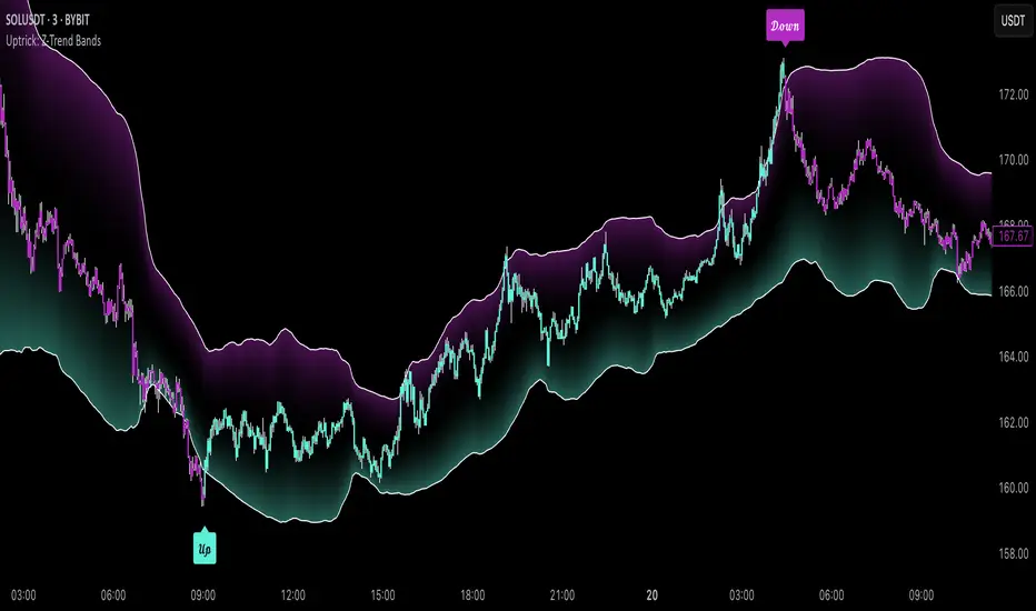
LANZ Strategy 4.0 [Backtest]🔷 LANZ Strategy 4.0 — Strategy Execution Based on Confirmed Structure + Risk-Based SL/TP
LANZ Strategy 4.0 is the official backtesting engine for the LANZ Strategy 4.0 trading logic. It simulates real-time executions based on breakout of Strong/Weak Highs or Lows, using a consistent structural system with SL/TP dynamically calculated per trade. With integrated risk management and lot size logic, this script allows traders to validate LANZ Strategy 4.0 performance with real strategy metrics.
🧠 Core Components:
Confirmed Breakout Entries: Trades are executed only when price breaks the most recent structural level (Strong High or Strong Low), detected using swing pivots.
Dynamic SL and TP Logic: SL is placed below/above the breakout point with a customizable buffer. TP is defined using a fixed Risk-Reward (RR) ratio.
Capital-Based Risk Management: Lot size is calculated based on account equity, SL distance, and pip value (e.g. $10 per pip on XAUUSD).
Clean and Controlled Executions: Only one trade is active at a time. No new entries are allowed until the current position is closed.
📊 Visual Features:
Automatic plotting of Entry, SL, and TP levels.
Full control of swing sensitivity (swingLength) and SL buffer.
SL and TP lines extend visually for clarity of trade risk and reward zones.
⚙️ How It Works:
Detects pivots and classifies trend direction.
Waits for breakout above Strong High (BUY) or below Strong Low (SELL).
Calculates dynamic SL and TP based on buffer and RR.
Computes trade size automatically based on risk per trade %.
Executes entry and manages exits via strategy engine.
📝 Notes:
Ideal for evaluating the LANZ Strategy 4.0 logic over historical data.
Must be paired with the original indicator (LANZ Strategy 4.0) for live trading.
Best used on assets with clear structural behavior (gold, indices, FX).
📌 Credits:
Backtest engine developed by LANZ based on the official rules of LANZ Strategy 4.0. This script ensures visual and logical consistency between live charting and backtesting simulations.
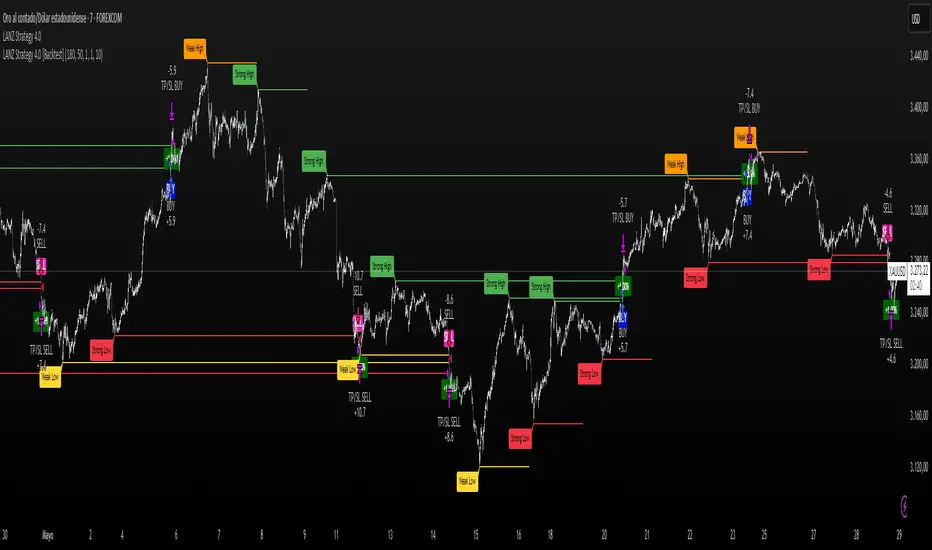
Hull Moving Average RibbonGradient Wave HMA - Multi-Ribbon Hull Moving Average System
Overview
The Gradient Wave HMA is an advanced technical indicator that transforms Alan Hull's Hull Moving Average (HMA) into a dynamic multi-layered ribbon system. Unlike traditional moving average ribbons that use simple or exponential calculations, this indicator applies Hull's innovative lag-reduction formula across 12 different timeframes simultaneously, creating a visually striking gradient effect that flows with market momentum.
Technical Foundation
This indicator is built upon the Hull Moving Average, developed by Alan Hull in 2005. The HMA uses a weighted moving average calculation designed to almost eliminate lag while maintaining curve smoothness:
HMA = WMA(2*WMA(n/2) − WMA(n), sqrt(n))
Credit: Alan Hull (www.alanhull.com)
Key Features
Multi-Period Ribbon Structure
12 individual HMA lines with customizable periods
Preset configurations for different trading styles:
Fast: 3-30 period range (scalping/intraday)
Swing: 8-55 period range (swing trading)
Position: 20-100 period range (position trading)
Custom: User-defined periods
2. Neon Gradient Visualization
Bullish Gradient: Transitions from blue-purple to hot purple
Bearish Gradient: Flows from hot pink to purple-pink
Each line has a unique color in the spectrum
Gradient fills between lines create depth and visual flow
3. Advanced Alert System
Trend Reversal Alerts: Notifies when ribbon changes direction
Price Breakout Alerts: Triggers when price crosses the ribbon
Compression Alerts: Signals potential breakouts during consolidation
Expansion Alerts: Confirms strong trending conditions
Momentum Surge Alerts: Catches explosive moves early
How It Works
The indicator calculates 12 Hull Moving Averages, each with a different period length. The trend direction is determined by the middle HMA (6th line), which triggers the color change across the entire ribbon. When trending up, the ribbon displays a purple gradient; when trending down, it shifts to a pink gradient.
Trading Applications
1. Trend Identification
Ribbon color indicates overall trend direction
All lines moving in sync confirms strong trend
Mixed signals suggest choppy or transitioning markets
2. Dynamic Support/Resistance
In uptrends, the ribbon acts as moving support
In downtrends, it provides resistance levels
Multiple layers offer various strength levels
3. Momentum Analysis
Expanding ribbon = Increasing momentum
Contracting ribbon = Decreasing momentum/consolidation
Ribbon angle indicates trend strength
4. Trading Example
Advantages Over Traditional MAs
Reduced Lag: Hull's formula provides faster response than SMA/EMA ribbons
Visual Clarity: Gradient effect makes trend changes immediately visible
Multiple Timeframes: 12 periods provide comprehensive market view
Flexibility: Presets adapt to different trading styles
Best Practices
Use higher timeframes (4H, Daily) for position trading
Combine with volume indicators for confirmation
Watch for ribbon compression before major moves
Consider overall market conditions when interpreting signals
Customization Options
Adjust individual HMA periods
Fine-tune transparency for different backgrounds
Choose between WMA and EMA base calculations
The Gradient Wave HMA combines Alan Hull's breakthrough moving average formula with modern visualization techniques to create a powerful trend-following tool that's both technically sophisticated and visually intuitive.

Interest Zones | @CRYPTOKAZANCEVEnglish Description.
🧠 What This Script Does
This script automatically detects price interest zones — areas where the price repeatedly reacts by forming local swing highs or lows , suggesting heightened supply/demand or market attention. It uses a custom volatility-adjusted range (pseudo-ATR) to dynamically group significant swing points and highlights these zones visually on the chart.
The script is not a mashup or copy of built-in indicators. It’s an original implementation that performs a meaningful calculation based on market structure and volatility to help traders identify important price areas.
⚙️ How It Works
1. Swing Point Detection:
The script identifies swing highs and lows using a configurable lookback window.
2. Zone Candidate Evaluation:
Each swing is checked against a custom zone width (based on ATR and your multiplier). If multiple swings fall within this range, it’s marked as a potential zone.
3. Filtering:
The script keeps only those zones that:
• Contain at least a user-defined number of swing points.
• Do not overlap with stronger (higher swing count) zones.
4. Visualization:
• The strongest zones are drawn as semi-transparent boxes.
• Zones are limited by time (last X candles).
• Optional: Swing highs/lows can be shown on chart.
📊 How to Use
• Use it on any timeframe or asset to identify price regions of interest.
• Combine with volume, trend, or candlestick analysis for entries/exits.
• The number of touches (swing points in a zone) gives insight into zone significance.
This tool is particularly useful for identifying support/resistance areas based on actual price structure rather than arbitrary levels.
🔧 Settings
• Swing Lookback Period: Controls how many candles on each side of a pivot the script checks to detect a local high/low.
• Zone Width Multiplier: Adjusts the volatility-based range. Larger values create wider zones.
• Min Swing Count: Zones with fewer swing points than this won't be shown.
• Max Zones Displayed: Limits the number of zones shown on screen.
• Max Candles for Analysis: Old swing points beyond this range are ignored.
📌 Notes
• No third-party code or mashups used.
• This is a standalone implementation of a concept similar to market structure mapping, tailored to be dynamic and responsive to volatility.
• Ideal for traders who prefer clean, price-action-based analysis.
🇷🇺 Русское описание
🧠 Что делает этот индикатор:
Индикатор автоматически определяет зоны интереса цены — области, где цена многократно формирует локальные максимумы или минимумы (свинги) . Эти зоны могут сигнализировать о повышенном внимании рынка, предложении или спросе. Скрипт использует псевдо-ATR (волатильность на основе среднего диапазона), чтобы динамически определять такие области и выделяет их на графике.
Это не копия стандартных индикаторов и не микс чужих скриптов — это оригинальная разработка , полезная для всех, кто ищет автоматическую разметку важных ценовых уровней.
⚙️ Как работает индикатор
1. Поиск свинг-точек:
Определяются локальные экстремумы с учетом указанного периода.
2. Формирование кандидатов в зоны:
Каждая свинг-точка проверяется, есть ли в её диапазоне другие свинги. Если таких достаточно — зона считается потенциальной.
3. Фильтрация зон:
• Учитываются только зоны с минимумом заданных свингов.
• Перекрывающиеся зоны удаляются в пользу более значимых.
4. Визуализация:
• Отображаются зоны с наибольшим числом касаний.
• Зоны ограничиваются последними X свечами.
• При желании можно отобразить сами свинг-точки.
📊 Как использовать
• Работает на любом таймфрейме и инструменте.
• Используйте совместно с объёмами, трендом или свечным анализом.
• Количество касаний помогает оценить важность зоны.
Полезен тем, кто предпочитает анализ на основе структуры цены, а не произвольных уровней.
🔧 Настройки
• Период свингов: Сколько свечей учитывается по бокам для поиска экстремумов.
• Множитель зоны: Увеличивает диапазон зоны на основе волатильности.
• Мин. количество свингов: Минимум точек в зоне для её отображения.
• Макс. зон на графике: Ограничение по количеству отображаемых зон.
• Макс. свечей анализа: Старые точки за пределами не учитываются.
📌 Примечания
• Не содержит чужих индикаторов или шаблонов.
• Самостоятельная реализация механизма анализа структуры рынка.

Enigma Sniper 369The "Enigma Sniper 369" is a custom-built Pine Script indicator designed for TradingView, tailored specifically for forex traders seeking high-probability entries during high-volatility market sessions.
Unlike generic trend-following or scalping tools, this indicator uniquely combines session-based "kill zones" (London and US sessions), momentum-based candle analysis, and an optional EMA trend filter to pinpoint liquidity grabs and reversal opportunities.
Its originality lies in its focus on liquidity hunting—identifying levels where stop losses are likely clustered (around swing highs/lows and wick midpoints)—and providing visual entry zones that are dynamically removed once price breaches them, reducing clutter and focusing on actionable signals.
The name "369" reflects the structured approach of three key components (session timing, candle logic, and trend filter) working in harmony to snipe precise entries.
What It Does
"Enigma Sniper 369" identifies potential buy and sell opportunities by drawing two types of horizontal lines on the chart during user-defined London and US
session kill zones:
Solid Lines: Mark the swing low (for buys) or swing high (for sells) of a trigger candle, indicating a potential entry point where stop losses might be clustered.
Dotted Lines: Mark the 50% level of the candle’s wick (lower wick for buys, upper wick for sells), serving as a secondary confirmation zone for entries or tighter stop-loss placement.
These lines are plotted only when specific candle conditions are met within the kill zones, and they are automatically deleted once the price crosses them, signaling that the liquidity at that level has likely been grabbed. The indicator also includes an optional EMA filter to ensure trades align with the broader trend, reducing false signals in choppy markets.
How It Works
The indicator’s logic is built on a multi-layered approach:
Kill Zone Timing: Trades are only considered during user-defined London and US session hours (e.g., London from 02:00 to 12:00 UTC, as seen in the screenshots). These sessions are known for high volatility and liquidity, making them ideal for capturing institutional moves.
Candle-Based Momentum Logic:
Buy Signal: A candle must close above its midpoint (indicating bullish momentum) and have a lower low than the previous candle (suggesting a potential liquidity grab below the previous swing low). This is expressed as close > (high + low) / 2 and low < low .
Sell Signal: A candle must close below its midpoint (bearish momentum) and have a higher high than the previous candle (indicating a potential liquidity grab above the previous swing high), expressed as close < (high + low) / 2 and high > high .
These conditions ensure the indicator targets candles that break recent structure to hunt stop losses while showing directional momentum.
Optional EMA Filter: A 50-period EMA (customizable) can be enabled to filter signals based on trend direction.
Buy signals are only generated if the EMA is trending upward (ema_value > ema_value ), and sell signals require a downward EMA trend (ema_value < ema_value ). This reduces noise by aligning entries with the broader market trend.
Liquidity Levels and Deletion Logic:
For a buy signal, a solid green line is drawn at the candle’s low, and a dotted green line at the 50% level of the lower wick (from the candle body’s bottom to the low).
For a sell signal, a solid red line is drawn at the candle’s high, and a dotted red line at the 50% level of the upper wick (from the body’s top to the high).
These lines extend to the right until the price crosses them, at which point they are deleted, indicating the liquidity at that level has been taken (e.g., stop losses triggered).
Alerts: The indicator includes alert conditions for buy and sell signals, notifying traders when a new setup is identified.
Underlying Concepts
The indicator is grounded in the concept of liquidity hunting, a strategy often employed by institutional traders. Markets frequently move to levels where stop losses are clustered—typically just beyond swing highs or lows—before reversing in the opposite direction. The "Enigma Sniper 369" targets these moves by identifying candles that break structure (e.g., a lower low or higher high) during high-volatility sessions, suggesting a potential sweep of stop losses. The 50% wick level acts as a secondary confirmation, as this midpoint often represents a zone where tighter stop losses are placed by retail traders. The optional EMA filter adds a trend-following element, ensuring entries are taken in the direction of the broader market momentum, which is particularly useful on lower timeframes like the 15-minute chart shown in the screenshots.
How to Use It
Here’s a step-by-step guide based on the provided usage example on the GBP/USD 15-minute chart:
Setup the Indicator: Add "Enigma Sniper 369" to your TradingView chart. Adjust the London and US session hours to match your timezone (e.g., London from 02:00 to 12:00 UTC, US from 13:00 to 22:00 UTC). Customize the EMA period (default 50) and line styles/colors if desired.
Identify Kill Zones: The indicator highlights the London session in light green and the US session in light purple, as seen in the screenshots. Focus on these periods for signals, as they are the most volatile and likely to produce liquidity grabs.
Wait for a Signal: Look for solid and dotted lines to appear during the kill zones:
Buy Setup: A solid green line at the swing low and a dotted green line at the 50% lower wick level indicate a potential buy. This suggests the market may have grabbed liquidity below the swing low and is now poised to move higher.
Sell Setup: A solid red line at the swing high and a dotted red line at the 50% upper wick level indicate a potential sell, suggesting liquidity was taken above the swing high.
Place Your Trade:
For a buy, set a buy limit order at the dotted green line (50% wick level), as this is a more conservative entry point. Place your stop loss just below the solid green line (swing low) to cover the full swing. For example, in the screenshots, the market retraces to the dotted line at 1.32980 after a liquidity grab below the swing low, triggering a buy limit order.
For a sell, set a sell limit order at the dotted red line, with a stop loss just above the solid red line.
Monitor Price Action: Once the price crosses a line, it is deleted, indicating the liquidity at that level has been taken. In the screenshots, after the buy limit is triggered, the market moves higher, confirming the setup. The caption notes, “The market returns and tags us in long with a buy limit,” highlighting this retracement strategy.
Additional Context: Use the indicator to identify liquidity levels that may be targeted later. For example, the screenshot notes, “If a new session is about to open I will wait for the grab liquidity to go long,” showing how the indicator can be used to anticipate future moves at session opens (e.g., London open at 1.32980).
Risk Management: Always set a stop loss below the swing low (for buys) or above the swing high (for sells) to protect against adverse moves. The 50% wick level helps tighten entries, improving the risk-reward ratio.
Practical Example
On the GBP/USD 15-minute chart, during the London session (02:00 UTC), the indicator identifies a buy setup with a solid green line at 1.32901 (swing low) and a dotted green line at 1.32980 (50% wick level). The market initially dips below the swing low, grabbing liquidity, then retraces to the dotted line, triggering a buy limit order. The price subsequently rises to 1.33404, yielding a profitable trade. The user notes, “The logic is in the last candle it provides new level to go long,” emphasizing the indicator’s ability to identify fresh levels after a liquidity sweep.
Customization Tips
Adjust the EMA period to suit your timeframe (e.g., a shorter period like 20 for faster signals on lower timeframes).
Modify the session hours to align with your broker’s timezone or specific market conditions.
Use the alert feature to get notified of new setups without constantly monitoring the chart.
Why It’s Useful for Traders
The "Enigma Sniper 369" stands out by combining session timing, momentum-based candle analysis, and liquidity hunting into a single tool. It provides clear, actionable levels for entries and stop losses, removes invalid signals dynamically, and aligns trades with high-probability market conditions. Whether you’re a scalper looking for quick moves during London open or a swing trader targeting session-based reversals, this indicator offers a structured, data-driven approach to trading.
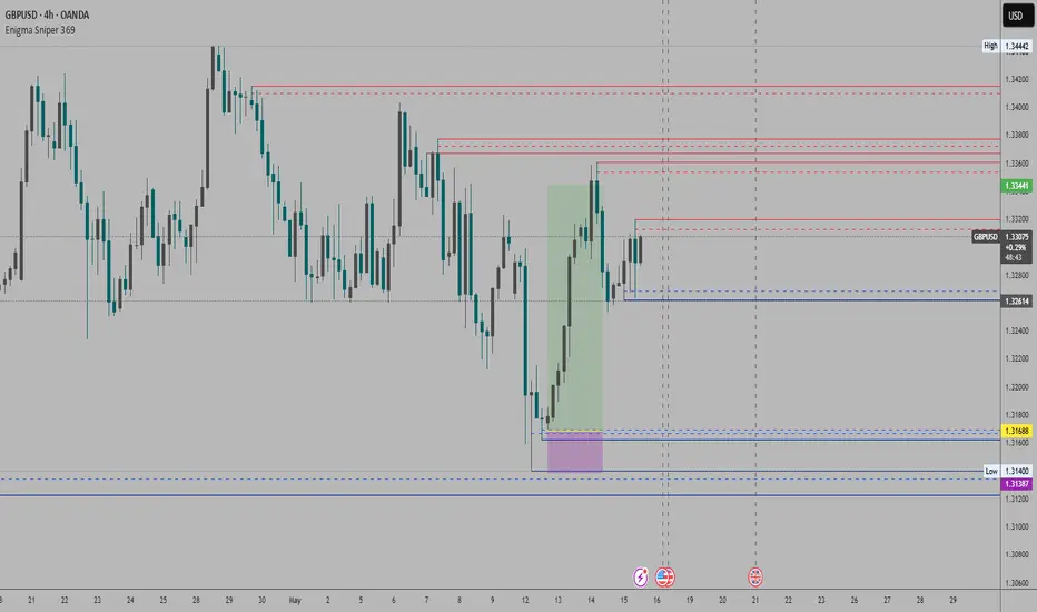
Bober XM v2.0# ₿ober XM v2.0 Trading Bot Documentation
**Developer's Note**: While our previous Bot 1.3.1 was removed due to guideline violations, this setback only fueled our determination to create something even better. Rising from this challenge, Bober XM 2.0 emerges not just as an update, but as a complete reimagining with multi-timeframe analysis, enhanced filters, and superior adaptability. This adversity pushed us to innovate further and deliver a strategy that's smarter, more agile, and more powerful than ever before. Challenges create opportunity - welcome to Cryptobeat's finest work yet.
## !!!!You need to tune it for your own pair and timeframe and retune it periodicaly!!!!!
## Overview
The ₿ober XM v2.0 is an advanced dual-channel trading bot with multi-timeframe analysis capabilities. It integrates multiple technical indicators, customizable risk management, and advanced order execution via webhook for automated trading. The bot's distinctive feature is its separate channel systems for long and short positions, allowing for asymmetric trade strategies that adapt to different market conditions across multiple timeframes.
### Key Features
- **Multi-Timeframe Analysis**: Analyze price data across multiple timeframes simultaneously
- **Dual Channel System**: Separate parameter sets for long and short positions
- **Advanced Entry Filters**: RSI, Volatility, Volume, Bollinger Bands, and KEMAD filters
- **Machine Learning Moving Average**: Adaptive prediction-based channels
- **Multiple Entry Strategies**: Breakout, Pullback, and Mean Reversion modes
- **Risk Management**: Customizable stop-loss, take-profit, and trailing stop settings
- **Webhook Integration**: Compatible with external trading bots and platforms
### Strategy Components
| Component | Description |
|---------|-------------|
| **Dual Channel Trading** | Uses either Keltner Channels or Machine Learning Moving Average (MLMA) with separate settings for long and short positions |
| **MLMA Implementation** | Machine learning algorithm that predicts future price movements and creates adaptive bands |
| **Pivot Point SuperTrend** | Trend identification and confirmation system based on pivot points |
| **Three Entry Strategies** | Choose between Breakout, Pullback, or Mean Reversion approaches |
| **Advanced Filter System** | Multiple customizable filters with multi-timeframe support to avoid false signals |
| **Custom Exit Logic** | Exits based on OBV crossover of its moving average combined with pivot trend changes |
### Note for Novice Users
This is a fully featured real trading bot and can be tweaked for any ticker — SOL is just an example. It follows this structure:
1. **Indicator** – gives the initial signal
2. **Entry strategy** – decides when to open a trade
3. **Exit strategy** – defines when to close it
4. **Trend confirmation** – ensures the trade follows the market direction
5. **Filters** – cuts out noise and avoids weak setups
6. **Risk management** – controls losses and protects your capital
To tune it for a different pair, you'll need to start from scratch:
1. Select the timeframe (candle size)
2. Turn off all filters and trend entry/exit confirmations
3. Choose a channel type, channel source and entry strategy
4. Adjust risk parameters
5. Tune long and short settings for the channel
6. Fine-tune the Pivot Point Supertrend and Main Exit condition OBV
This will generate a lot of signals and activity on the chart. Your next task is to find the right combination of filters and settings to reduce noise and tune it for profitability.
### Default Strategy values
Default values are tuned for: Symbol BITGET:SOLUSDT.P 5min candle
Filters are off by default: Try to play with it to understand how it works
## Configuration Guide
### General Settings
| Setting | Description | Default Value |
|---------|-------------|---------------|
| **Long Positions** | Enable or disable long trades | Enabled |
| **Short Positions** | Enable or disable short trades | Enabled |
| **Risk/Reward Area** | Visual display of stop-loss and take-profit zones | Enabled |
| **Long Entry Source** | Price data used for long entry signals | hl2 (High+Low/2) |
| **Short Entry Source** | Price data used for short entry signals | hl2 (High+Low/2) |
The bot allows you to trade long positions, short positions, or both simultaneously. Each direction has its own set of parameters, allowing for fine-tuned strategies that recognize the asymmetric nature of market movements.
### Multi-Timeframe Settings
1. **Enable Multi-Timeframe Analysis**: Toggle 'Enable Multi-Timeframe Analysis' in the Multi-Timeframe Settings section
2. **Configure Timeframes**: Set appropriate higher timeframes based on your trading style:
- Timeframe 1: Default is now 15 minutes (intraday confirmation)
- Timeframe 2: Default is 4 hours (trend direction)
3. **Select Sources per Indicator**: For each indicator (RSI, KEMAD, Volume, etc.), choose:
- The desired timeframe (current, mtf1, or mtf2)
- The appropriate price type (open, high, low, close, hl2, hlc3, ohlc4)
### Entry Strategies
- **Breakout**: Enter when price breaks above/below the channel
- **Pullback**: Enter when price pulls back to the channel
- **Mean Reversion**: Enter when price is extended from the channel
You can enable different strategies for long and short positions.
### Core Components
### Risk Management
- **Position Size**: Control risk with percentage-based position sizing
- **Stop Loss Options**:
- Fixed: Set a specific price or percentage from entry
- ATR-based: Dynamic stop-loss based on market volatility
- Swing: Uses recent swing high/low points
- **Take Profit**: Multiple targets with percentage allocation
- **Trailing Stop**: Dynamic stop that follows price movement
## Advanced Usage Strategies
### Moving Average Type Selection Guide
- **SMA**: More stable in choppy markets, good for higher timeframes
- **EMA/WMA**: More responsive to recent price changes, better for entry signals
- **VWMA**: Adds volume weighting for stronger trends, use with Volume filter
- **HMA**: Balance between responsiveness and noise reduction, good for volatile markets
### Multi-Timeframe Strategy Approaches
- **Trend Confirmation**: Use higher timeframe RSI (mtf2) for overall trend, current timeframe for entries
- **Entry Precision**: Use KEMAD on current timeframe with volume filter on mtf1
- **False Signal Reduction**: Apply RSI filter on mtf1 with strict KEMAD settings
### Market Condition Optimization
| Market Condition | Recommended Settings |
|------------------|----------------------|
| **Trending** | Use Breakout strategy with KEMAD filter on higher timeframe |
| **Ranging** | Use Mean Reversion with strict RSI filter (mtf1) |
| **Volatile** | Increase ATR multipliers, use HMA for moving averages |
| **Low Volatility** | Decrease noise parameters, use pullback strategy |
## Webhook Integration
The strategy features a professional webhook system that allows direct connectivity to your exchange or trading platform of choice through third-party services like 3commas, Alertatron, or Autoview.
The webhook payload includes all necessary parameters for automated execution:
- Entry price and direction
- Stop loss and take profit levels
- Position size
- Custom identifier for webhook routing
## Performance Optimization Tips
1. **Start with Defaults**: Begin with the default settings for your timeframe before customizing
2. **Adjust One Component at a Time**: Make incremental changes and test the impact
3. **Match MA Types to Market Conditions**: Use appropriate moving average types based on the Market Condition Optimization table
4. **Timeframe Synergy**: Create logical relationships between timeframes (e.g., 5min chart with 15min and 4h higher timeframes)
5. **Periodic Retuning**: Markets evolve - regularly review and adjust parameters
## Common Setups
### Crypto Trend-Following
- MLMA with EMA or HMA
- Higher RSI thresholds (75/25)
- KEMAD filter on mtf1
- Breakout entry strategy
### Stock Swing Trading
- MLMA with SMA for stability
- Volume filter with higher threshold
- KEMAD with increased filter order
- Pullback entry strategy
### Forex Scalping
- MLMA with WMA and lower noise parameter
- RSI filter on current timeframe
- Use highest timeframe for trend direction only
- Mean Reversion strategy
## Webhook Configuration
- **Benefits**:
- Automated trade execution without manual intervention
- Immediate response to market conditions
- Consistent execution of your strategy
- **Implementation Notes**:
- Requires proper webhook configuration on your exchange or platform
- Test thoroughly with small position sizes before full deployment
- Consider latency between signal generation and execution
### Backtesting Period
Define a specific historical period to evaluate the bot's performance:
| Setting | Description | Default Value |
|---------|-------------|---------------|
| **Start Date** | Beginning of backtest period | January 1, 2025 |
| **End Date** | End of backtest period | December 31, 2026 |
- **Best Practice**: Test across different market conditions (bull markets, bear markets, sideways markets)
- **Limitation**: Past performance doesn't guarantee future results
## Entry and Exit Strategies
### Dual-Channel System
A key innovation of the Bober XM is its dual-channel approach:
- **Independent Parameters**: Each trade direction has its own channel settings
- **Asymmetric Trading**: Recognizes that markets often behave differently in uptrends versus downtrends
- **Optimized Performance**: Fine-tune settings for both bullish and bearish conditions
This approach allows the bot to adapt to the natural asymmetry of markets, where uptrends often develop gradually while downtrends can be sharp and sudden.
### Channel Types
#### 1. Keltner Channels
Traditional volatility-based channels using EMA and ATR:
| Setting | Long Default | Short Default |
|---------|--------------|---------------|
| **EMA Length** | 37 | 20 |
| **ATR Length** | 13 | 17 |
| **Multiplier** | 1.4 | 1.9 |
| **Source** | low | high |
- **Strengths**:
- Reliable in trending markets
- Less prone to whipsaws than Bollinger Bands
- Clear visual representation of volatility
- **Weaknesses**:
- Can lag during rapid market changes
- Less effective in choppy, non-trending markets
#### 2. Machine Learning Moving Average (MLMA)
Advanced predictive model using kernel regression (RBF kernel):
| Setting | Description | Options |
|---------|-------------|--------|
| **Source MA** | Price data used for MA calculations | Any price source (low/high/close/etc.) |
| **Moving Average Type** | Type of MA algorithm for calculations | SMA, EMA, WMA, VWMA, RMA, HMA |
| **Trend Source** | Price data used for trend determination | Any price source (close default) |
| **Window Size** | Historical window for MLMA calculations | 5+ (default: 16) |
| **Forecast Length** | Number of bars to forecast ahead | 1+ (default: 3) |
| **Noise Parameter** | Controls smoothness of prediction | 0.01+ (default: ~0.43) |
| **Band Multiplier** | Multiplier for channel width | 0.1+ (default: 0.5-0.6) |
- **Strengths**:
- Predictive rather than reactive
- Adapts quickly to changing market conditions
- Better at identifying trend reversals early
- **Weaknesses**:
- More computationally intensive
- Requires careful parameter tuning
- Can be sensitive to input data quality
### Entry Strategies
| Strategy | Description | Ideal Market Conditions |
|----------|-------------|-------------------------|
| **Breakout** | Enters when price breaks through channel bands, indicating strong momentum | High volatility, emerging trends |
| **Pullback** | Enters when price retraces to the middle band after testing extremes | Established trends with regular pullbacks |
| **Mean Reversion** | Enters at channel extremes, betting on a return to the mean | Range-bound or oscillating markets |
#### Breakout Strategy (Default)
- **Implementation**: Enters long when price crosses above the upper band, short when price crosses below the lower band
- **Strengths**: Captures strong momentum moves, performs well in trending markets
- **Weaknesses**: Can lead to late entries, higher risk of false breakouts
- **Optimization Tips**:
- Increase channel multiplier for fewer but more reliable signals
- Combine with volume confirmation for better accuracy
#### Pullback Strategy
- **Implementation**: Enters long when price pulls back to middle band during uptrend, short during downtrend pullbacks
- **Strengths**: Better entry prices, lower risk, higher probability setups
- **Weaknesses**: Misses some strong moves, requires clear trend identification
- **Optimization Tips**:
- Use with trend filters to confirm overall direction
- Adjust middle band calculation for market volatility
#### Mean Reversion Strategy
- **Implementation**: Enters long at lower band, short at upper band, expecting price to revert to the mean
- **Strengths**: Excellent entry prices, works well in ranging markets
- **Weaknesses**: Dangerous in strong trends, can lead to fighting the trend
- **Optimization Tips**:
- Implement strong trend filters to avoid counter-trend trades
- Use smaller position sizes due to higher risk nature
### Confirmation Indicators
#### Pivot Point SuperTrend
Combines pivot points with ATR-based SuperTrend for trend confirmation:
| Setting | Default Value |
|---------|---------------|
| **Pivot Period** | 25 |
| **ATR Factor** | 2.2 |
| **ATR Period** | 41 |
- **Function**: Identifies significant market turning points and confirms trend direction
- **Implementation**: Requires price to respect the SuperTrend line for trade confirmation
#### Weighted Moving Average (WMA)
Provides additional confirmation layer for entries:
| Setting | Default Value |
|---------|---------------|
| **Period** | 15 |
| **Source** | ohlc4 (average of Open, High, Low, Close) |
- **Function**: Confirms trend direction and filters out low-quality signals
- **Implementation**: Price must be above WMA for longs, below for shorts
### Exit Strategies
#### On-Balance Volume (OBV) Based Exits
Uses volume flow to identify potential reversals:
| Setting | Default Value |
|---------|---------------|
| **Source** | ohlc4 |
| **MA Type** | HMA (Options: SMA, EMA, WMA, RMA, VWMA, HMA) |
| **Period** | 22 |
- **Function**: Identifies divergences between price and volume to exit before reversals
- **Implementation**: Exits when OBV crosses its moving average in the opposite direction
- **Customizable MA Type**: Different MA types provide varying sensitivity to OBV changes:
- **SMA**: Traditional simple average, equal weight to all periods
- **EMA**: More weight to recent data, responds faster to price changes
- **WMA**: Weighted by recency, smoother than EMA
- **RMA**: Similar to EMA but smoother, reduces noise
- **VWMA**: Factors in volume, helpful for OBV confirmation
- **HMA**: Reduces lag while maintaining smoothness (default)
#### ADX Exit Confirmation
Uses Average Directional Index to confirm trend exhaustion:
| Setting | Default Value |
|---------|---------------|
| **ADX Threshold** | 35 |
| **ADX Smoothing** | 60 |
| **DI Length** | 60 |
- **Function**: Confirms trend weakness before exiting positions
- **Implementation**: Requires ADX to drop below threshold or DI lines to cross
## Filter System
### RSI Filter
- **Function**: Controls entries based on momentum conditions
- **Parameters**:
- Period: 15 (default)
- Overbought level: 71
- Oversold level: 23
- Multi-timeframe support: Current, MTF1 (15min), or MTF2 (4h)
- Customizable price source (open, high, low, close, hl2, hlc3, ohlc4)
- **Implementation**: Blocks long entries when RSI > overbought, short entries when RSI < oversold
### Volatility Filter
- **Function**: Prevents trading during excessive market volatility
- **Parameters**:
- Measure: ATR (Average True Range)
- Period: Customizable (default varies by timeframe)
- Threshold: Adjustable multiplier
- Multi-timeframe support
- Customizable price source
- **Implementation**: Blocks trades when current volatility exceeds threshold × average volatility
### Volume Filter
- **Function**: Ensures adequate market liquidity for trades
- **Parameters**:
- Threshold: 0.4× average (default)
- Measurement period: 5 (default)
- Moving average type: Customizable (HMA default)
- Multi-timeframe support
- Customizable price source
- **Implementation**: Requires current volume to exceed threshold × average volume
### Bollinger Bands Filter
- **Function**: Controls entries based on price relative to statistical boundaries
- **Parameters**:
- Period: Customizable
- Standard deviation multiplier: Adjustable
- Moving average type: Customizable
- Multi-timeframe support
- Customizable price source
- **Implementation**: Can require price to be within bands or breaking out of bands depending on strategy
### KEMAD Filter (Kalman EMA Distance)
- **Function**: Advanced trend confirmation using Kalman filter algorithm
- **Parameters**:
- Process Noise: 0.35 (controls smoothness)
- Measurement Noise: 24 (controls reactivity)
- Filter Order: 6 (higher = more smoothing)
- ATR Length: 8 (for bandwidth calculation)
- Upper Multiplier: 2.0 (for long signals)
- Lower Multiplier: 2.7 (for short signals)
- Multi-timeframe support
- Customizable visual indicators
- **Implementation**: Generates signals based on price position relative to Kalman-filtered EMA bands
## Risk Management System
### Position Sizing
Automatically calculates position size based on account equity and risk parameters:
| Setting | Default Value |
|---------|---------------|
| **Risk % of Equity** | 50% |
- **Implementation**:
- Position size = (Account equity × Risk %) ÷ (Entry price × Stop loss distance)
- Adjusts automatically based on volatility and stop placement
- **Best Practices**:
- Start with lower risk percentages (1-2%) until strategy is proven
- Consider reducing risk during high volatility periods
### Stop-Loss Methods
Multiple stop-loss calculation methods with separate configurations for long and short positions:
| Method | Description | Configuration |
|--------|-------------|---------------|
| **ATR-Based** | Dynamic stops based on volatility | ATR Period: 14, Multiplier: 2.0 |
| **Percentage** | Fixed percentage from entry | Long: 1.5%, Short: 1.5% |
| **PIP-Based** | Fixed currency unit distance | 10.0 pips |
- **Implementation Notes**:
- ATR-based stops adapt to changing market volatility
- Percentage stops maintain consistent risk exposure
- PIP-based stops provide precise control in stable markets
### Trailing Stops
Locks in profits by adjusting stop-loss levels as price moves favorably:
| Setting | Default Value |
|---------|---------------|
| **Stop-Loss %** | 1.5% |
| **Activation Threshold** | 2.1% |
| **Trailing Distance** | 1.4% |
- **Implementation**:
- Initial stop remains fixed until profit reaches activation threshold
- Once activated, stop follows price at specified distance
- Locks in profit while allowing room for normal price fluctuations
### Risk-Reward Parameters
Defines the relationship between risk and potential reward:
| Setting | Default Value |
|---------|---------------|
| **Risk-Reward Ratio** | 1.4 |
| **Take Profit %** | 2.4% |
| **Stop-Loss %** | 1.5% |
- **Implementation**:
- Take profit distance = Stop loss distance × Risk-reward ratio
- Higher ratios require fewer winning trades for profitability
- Lower ratios increase win rate but reduce average profit
### Filter Combinations
The strategy allows for simultaneous application of multiple filters:
- **Recommended Combinations**:
- Trending markets: RSI + KEMAD filters
- Ranging markets: Bollinger Bands + Volatility filters
- All markets: Volume filter as minimum requirement
- **Performance Impact**:
- Each additional filter reduces the number of trades
- Quality of remaining trades typically improves
- Optimal combination depends on market conditions and timeframe
### Multi-Timeframe Filter Applications
| Filter Type | Current Timeframe | MTF1 (15min) | MTF2 (4h) |
|-------------|-------------------|-------------|------------|
| RSI | Quick entries/exits | Intraday trend | Overall trend |
| Volume | Immediate liquidity | Sustained support | Market participation |
| Volatility | Entry timing | Short-term risk | Regime changes |
| KEMAD | Precise signals | Trend confirmation | Major reversals |
## Visual Indicators and Chart Analysis
The bot provides comprehensive visual feedback on the chart:
- **Channel Bands**: Keltner or MLMA bands showing potential support/resistance
- **Pivot SuperTrend**: Colored line showing trend direction and potential reversal points
- **Entry/Exit Markers**: Annotations showing actual trade entries and exits
- **Risk/Reward Zones**: Visual representation of stop-loss and take-profit levels
These visual elements allow for:
- Real-time strategy assessment
- Post-trade analysis and optimization
- Educational understanding of the strategy logic
## Implementation Guide
### TradingView Setup
1. Load the script in TradingView Pine Editor
2. Apply to your preferred chart and timeframe
3. Adjust parameters based on your trading preferences
4. Enable alerts for webhook integration
### Webhook Integration
1. Configure webhook URL in TradingView alerts
2. Set up receiving endpoint on your trading platform
3. Define message format matching the bot's output
4. Test with small position sizes before full deployment
### Optimization Process
1. Backtest across different market conditions
2. Identify parameter sensitivity through multiple tests
3. Focus on risk management parameters first
4. Fine-tune entry/exit conditions based on performance metrics
5. Validate with out-of-sample testing
## Performance Considerations
### Strengths
- Adaptability to different market conditions through dual channels
- Multiple layers of confirmation reducing false signals
- Comprehensive risk management protecting capital
- Machine learning integration for predictive edge
### Limitations
- Complex parameter set requiring careful optimization
- Potential over-optimization risk with so many variables
- Computational intensity of MLMA calculations
- Dependency on proper webhook configuration for execution
### Best Practices
- Start with conservative risk settings (1-2% of equity)
- Test thoroughly in demo environment before live trading
- Monitor performance regularly and adjust parameters
- Consider market regime changes when evaluating results
## Conclusion
The ₿ober XM v2.0 represents a significant evolution in trading strategy design, combining traditional technical analysis with machine learning elements and multi-timeframe analysis. The core strength of this system lies in its adaptability and recognition of market asymmetry.
### Market Asymmetry and Adaptive Approach
The strategy acknowledges a fundamental truth about markets: bullish and bearish phases behave differently and should be treated as distinct environments. The dual-channel system with separate parameters for long and short positions directly addresses this asymmetry, allowing for optimized performance regardless of market direction.
### Targeted Backtesting Philosophy
It's counterproductive to run backtests over excessively long periods. Markets evolve continuously, and strategies that worked in previous market regimes may be ineffective in current conditions. Instead:
- Test specific market phases separately (bull markets, bear markets, range-bound periods)
- Regularly re-optimize parameters as market conditions change
- Focus on recent performance with higher weight than historical results
- Test across multiple timeframes to ensure robustness
### Multi-Timeframe Analysis as a Game-Changer
The integration of multi-timeframe analysis fundamentally transforms the strategy's effectiveness:
- **Increased Safety**: Higher timeframe confirmations reduce false signals and improve trade quality
- **Context Awareness**: Decisions made with awareness of larger trends reduce adverse entries
- **Adaptable Precision**: Apply strict filters on lower timeframes while maintaining awareness of broader conditions
- **Reduced Noise**: Higher timeframe data naturally filters market noise that can trigger poor entries
The ₿ober XM v2.0 provides traders with a framework that acknowledges market complexity while offering practical tools to navigate it. With proper setup, realistic expectations, and attention to changing market conditions, it delivers a sophisticated approach to systematic trading that can be continuously refined and optimized.
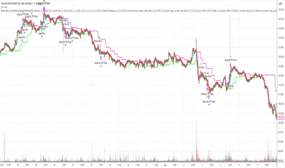
LANZ Strategy 2.0🔷 LANZ Strategy 2.0 — London Breakout Confirmation with Structural Swing Protection
LANZ Strategy 2.0 is a structured trading system that leverages the last confirmed market direction before the London session to define directional bias and manage trades based on key structural swing levels. It is tailored for intraday traders looking to capitalize on early London volatility with built-in risk management and visual clarity.
🧠 Core Components:
Directional Confirmation (Pre-London Bias): Validates the last breakout or structural move from the 15-minute timeframe before 02:15 a.m. New York time (start of the London session), establishing the expected market direction.
Time-Based Execution: Executes potential entries strictly at 02:15 a.m. NY time, using market structure to support Long or Short bias.
Dynamic Swing-Based SL System: Allows user to select between three SL protection models: First Swing (most recent structural point) Second Swing (prior level) Total Coverage (includes both swings + extra buffer) This supports flexibility based on trader profile or market conditions.
Visual Risk Mapping: All SL and TP levels are clearly plotted.
End-of-Session Management: Positions are automatically evaluated for closure at 11:45 a.m. NY time. SL, TP, or manual close outcomes are labeled accordingly.
📊 Visual Features:
Labels for 1st and 2nd swing levels upon entry.
Dynamic lines projecting SL/TP levels toward the end of the session.
Session background coloring for Pre-London, Execution, and NY sessions.
Real-time percentage outcome labels (+2.00%, -1.00%, or net % at session end).
Automatic deletion of previous visuals on new entries for clean charting.
⚙️ How It Works:
Detects last structural breakout on the 15m timeframe before 02:15 a.m. NY.
On the 02:15 a.m. candle, executes a Long or Short logic entry.
Plots corresponding SL and TP based on selected swing model.
Monitors price action: If TP or SL is hit, labels it accordingly. If no exit is hit, trade closes manually at 11:45 a.m. NY with net result shown.
Optional logic to reverse entries if market structure breaks before execution.
🔔 Alerts:
Daily execution alert at 02:15 a.m. NY (prompting manual review or action).
Optional alert logic can be extended for SL/TP hits or structure breaks.
📝 Notes:
Designed for semi-automated or discretionary intraday trading.
Best used on Forex pairs or indices with strong London session behavior.
Adjustable parameters include session hours, swing SL type, and buffer settings.
Credits:
Developed by LANZ, this script combines time-based execution with dynamic structure protection, offering a disciplined framework for participating in the London session breakout with clear visuals and risk logic.

Guppy Multiple Moving Average (GMMA)The GMMA Momentum Indicator plots 12 EMAs on your chart, divided into two groups:
Short-term EMAs (6 lines, default periods: 3, 5, 8, 10, 12, 15): Represent short-term trader sentiment and momentum.
Long-term EMAs (6 lines, default periods: 30, 35, 40, 45, 50, 60): Reflect long-term investor behavior and broader market trends.
By analyzing the interaction between these two groups, the indicator identifies:
Bullish and bearish trends based on the relative positions of the short- and long-term EMAs.
Momentum strength through the spread or convergence of the EMAs.
Potential reversals or breakouts via compression signals.
This PineScript version enhances the traditional GMMA by adding visual cues like background colors, bearish signals, and compression detection, making it ideal for swing traders seeking clear, actionable insights.
The GMMA Momentum Indicator provides several key features:
1. Trend Identification
Bullish Trend: When the short-term EMAs (green lines) are above the long-term EMAs (blue lines) and spreading apart, it signals strong upward momentum. The chart background turns light green to highlight this condition.
Bearish Trend: When the short-term EMAs cross below the long-term EMAs and converge, it indicates downward momentum. The background turns light red, and an orange downward triangle appears above the bar to mark a new bearish signal.
2. Momentum Analysis
The spread between the short-term EMAs reflects the strength of short-term momentum. A wide spread suggests strong momentum, while a tight grouping indicates weakening momentum or consolidation. Similarly, the long-term EMAs act as dynamic support or resistance, guiding traders on the broader trend.
3. Compression Detection
Compression occurs when both the short-term and long-term EMAs converge, signaling low volatility and a potential breakout or reversal. A yellow upward triangle appears below the bar when compression is detected, alerting traders to watch for price action.
4. Visual Cues
Green short-term EMAs: Show short-term trader activity.
Blue long-term EMAs: Represent long-term investor sentiment.
Background colors: Light green for bullish trends, light red for bearish trends, and transparent for neutral conditions.
Orange downward triangles: Mark new bearish trends.
Yellow upward triangles: Indicate compression, hinting at potential breakouts.
How to Use the GMMA Momentum Indicator for Swing Trading
Swing trading involves capturing price moves over days to weeks, and the GMMA Momentum Indicator is an excellent tool for this strategy. Here’s how to use it effectively:
1. Identifying Trade Entries
Buy Opportunities:
Look for a bullish trend (green background) where the short-term EMAs are above the long-term EMAs and spreading apart, indicating strong momentum.
A compression signal (yellow triangle) followed by a breakout above resistance or a bullish candlestick pattern can confirm an entry.
Example: On a daily chart, if the short-term EMAs cross above the long-term EMAs and the background turns green, consider entering a long position, especially if volume supports the move.
Sell Opportunities:
Watch for a bearish signal (orange downward triangle) or a bearish trend (red background) where the short-term EMAs cross below the long-term EMAs.
Example: If the short-term EMAs collapse below the long-term EMAs and an orange triangle appears, it may signal a shorting opportunity or a time to exit longs.
2. Managing Trades
Use the long-term EMAs as dynamic support (in uptrends) or resistance (in downtrends) to set stop-loss levels or trail stops.
Monitor the spread of the short-term EMAs. A widening spread suggests the trend is strong, while convergence may indicate it’s time to take profits or tighten stops.
3. Anticipating Reversals
Compression signals (yellow triangles) highlight periods of low volatility, often preceding significant price moves. Combine these with price action (e.g., breakouts or reversals) or other indicators (e.g., RSI or volume) for confirmation.
Example: If a compression signal appears near a key support level and the price breaks upward, it could signal the start of a new bullish swing.
4. Best Practices
Timeframes: The indicator works well on daily or 4-hour charts for swing trading, but you can adjust the EMA periods for shorter (e.g., 1-hour) or longer (e.g., weekly) timeframes.
Confirmation: Combine the GMMA with other tools like support/resistance levels, candlestick patterns, or oscillators (e.g., MACD) to reduce false signals.
Risk Management: Always use proper position sizing and stop-losses, as EMAs are lagging indicators and may produce delayed signals in choppy markets.
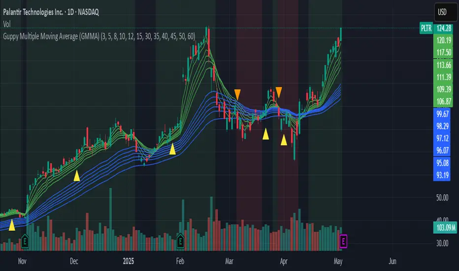
OTE & A-B-C Zone Indicator SwiftEdgeOTE & A-B-C Zone Indicator SwiftEdge
Overview
The OTE & A-B-C Zone Indicator SwiftEdge is a versatile tool designed to help traders identify high-probability trading setups using a combination of Optimal Trade Entry (OTE) zones, Fibonacci levels, and A-B-C price patterns. This indicator is particularly useful for traders who rely on price action and Fibonacci-based strategies to find entry points, set stop-losses, and target potential take-profit levels. By integrating swing point detection, trend analysis, and Fibonacci projections, SwiftEdge provides a clear visual framework for making informed trading decisions across various timeframes.
What It Does
SwiftEdge identifies key price levels and zones to guide your trading:
OTE Zone: Highlights the Optimal Trade Entry zone between swing points A (swing high) and B (swing low) using Fibonacci retracement levels (default: 0.618 to 0.786). This zone represents a high-probability area for price reversals, making it an ideal entry point for trades.
A-B-C Pattern: Marks the latest swing points as A (swing high), B (swing low), and C (projected take-profit level) with dashed lines and labels. A solid line connects A to B to C, visually illustrating the price movement from entry to target.
Take-Profit Zones: Projects three customizable take-profit levels (TP1, TP2, TP3) based on Fibonacci extensions (default: 1.272, 1.618, 2.0) from the A-B swing, helping traders plan exits with favorable risk-reward ratios.
How It Works
SwiftEdge combines several technical components to create a cohesive trading system:
Swing Point Detection: Identifies significant swing highs (A) and swing lows (B) using a dynamic lookback period that adjusts to the selected timeframe. On lower timeframes like 1-minute charts, an ATR-based filter reduces noise by requiring price movements to exceed a threshold (0.5 * ATR(14)).
Trend Analysis: Uses an Exponential Moving Average (EMA) to determine the trend direction (default: 50-period EMA on 1H). The indicator marks uptrends (price above EMA) in green and downtrends (price below EMA) in red, ensuring trades align with the market's direction.
Fibonacci Levels: Applies Fibonacci retracement to define the OTE zone between A and B, and Fibonacci extensions to project take-profit levels (C) beyond the initial swing. This approach leverages the natural tendency of markets to respect Fibonacci ratios for reversals and extensions.
Visual Clarity: Displays only the latest A-B-C pattern with three dashed lines (A, B, C) and a solid connecting line, ensuring the chart remains uncluttered and easy to interpret.
The combination of these elements creates a structured setup where the OTE zone (between A and B) serves as an entry point, while the projected C level offers a target, all within the context of the prevailing trend. This synergy makes SwiftEdge a powerful tool for traders seeking to combine price action, trend analysis, and Fibonacci strategies.
How to Use
Add the Indicator: Apply the indicator to your chart via TradingView's indicator menu.
Identify the Trend: The OTE zone and A-B-C pattern will be colored green in uptrends (price above EMA) or red in downtrends (price below EMA). Use this to determine the market direction.
Entry Point: Look for price reversals within the OTE zone (between A and B). This zone is typically between the 0.618 and 0.786 Fibonacci retracement levels of the A-B swing, making it a high-probability area for entries.
Stop-Loss: Place your stop-loss below the OTE zone in an uptrend (or above in a downtrend) to protect against false breakouts.
Take-Profit Targets: Use the projected take-profit zones (TP1, TP2, TP3) as potential exit levels. These are based on Fibonacci extensions and can be toggled on/off in the settings.
Customization:
Adjust the Fibonacci levels for the OTE zone (Fibonacci Level 1 and Fibonacci Level 2) to suit your strategy.
Modify the take-profit levels (Fibonacci Extension Level for TP1/TP2/TP3) to target different extension ratios.
Change the lookback period (Base Lookback Period) and EMA period (Base EMA Period) to fine-tune swing point detection and trend sensitivity.
Customize colors for uptrends, downtrends, and A-B-C lines to match your preferences.
What Makes It Unique
SwiftEdge stands out by integrating swing point detection, Fibonacci-based OTE zones, and A-B-C price patterns into a single, visually intuitive indicator. Unlike standalone Fibonacci tools or trend indicators, SwiftEdge combines these elements to provide a complete trading setup: it identifies entry zones (OTE), confirms trend direction (EMA), and projects take-profit targets (Fibonacci extensions). The dynamic timeframe adjustment ensures consistent performance across all chart intervals, while the clean A-B-C visualization (with only the latest pattern displayed) prevents chart clutter, making it easier to focus on the most relevant price levels.
Notes
This indicator is designed for traders familiar with price action and Fibonacci strategies. It does not guarantee profits and should be used in conjunction with other analysis tools and proper risk management.
Performance may vary depending on market conditions and timeframe. Test the indicator on a demo account before using it in live trading.
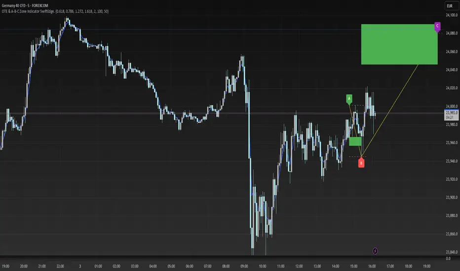
90-Day Beta to BTCOverview:
The 90-Day Beta to BTC indicator measures the volatility of a specific token relative to Bitcoin (BTC) over the past 90 days. Beta is a widely used statistical measure in financial markets that indicates how much a token's price moves in relation to BTC. A higher beta means the token is more volatile compared to BTC, while a lower beta means it is less volatile or moves similarly to BTC.
How It Works:
This indicator calculates the daily logarithmic returns of both the token and Bitcoin, then computes the covariance between their returns and the variance of Bitcoin’s returns. The resulting Beta value reflects the degree to which the token’s price fluctuates relative to Bitcoin's price over the past 90 days.
Beta > 1: The token is more volatile than Bitcoin, showing higher price swings.
Beta = 1: The token moves in lockstep with Bitcoin, exhibiting similar volatility.
Beta < 1: The token is less volatile than Bitcoin, showing smaller price fluctuations.
Beta = 0: The token's price movement is uncorrelated with Bitcoin’s price.
Negative Beta: The token moves opposite to Bitcoin, indicating an inverse relationship.
Use Case:
This indicator is particularly useful for traders or investors looking to identify tokens with high speculative volatility. Tokens with Beta values above 1 are typically high-risk, high-reward assets, often driven by hype, social trends, or market speculation. Conversely, tokens with Beta values below 1 offer a more stable price relationship with Bitcoin, making them less volatile and potentially safer.
In the context of a Trash Token Tournament, tokens with a higher Beta (greater than 1) may be more attractive due to their heightened volatility and potential for larger price swings, making them the “wild cards” of the market.
Visual Representation:
The Beta value is plotted as a line chart beneath the main price chart, offering a visual representation of the token’s volatility relative to Bitcoin over the last 90 days. Spikes in Beta indicate periods of increased volatility, while drops suggest stability.
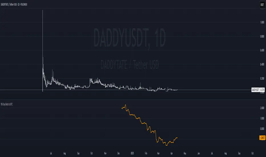
Quarterly Theory ICT 04 [TradingFinder] SSMT 4Quarter Divergence🔵 Introduction
Sequential SMT Divergence is an advanced price-action-based analytical technique rooted in the ICT (Inner Circle Trader) methodology. Its primary objective is to identify early-stage divergences between correlated assets within precise time structures. This tool not only breaks down market structure but also enables traders to detect engineered liquidity traps before the market reacts.
In simple terms, SMT (Smart Money Technique) occurs when two correlated assets—such as indices (ES and NQ), currency pairs (EURUSD and GBPUSD), or commodities (Gold and Silver)—exhibit different reactions at key price levels (swing highs or lows). This lack of alignment is often a sign of smart money manipulation and signals a lack of confirmation in the ongoing trend—hinting at an imminent reversal or at least a pause in momentum.
In its Sequential form, SMT divergences are examined through a more granular temporal lens—between intraday quarters (Q1 through Q4). When SMT appears at the transition from one quarter to another (e.g., Q1 to Q2 or Q3 to Q4), the signal becomes significantly more powerful, often aligning with a critical phase in the Quarterly Theory—a framework that segments market behavior into four distinct phases: Accumulation, Manipulation, Distribution, and Reversal/Continuation.
For instance, a Bullish SMT forms when one asset prints a new low while its correlated counterpart fails to break the corresponding low from the previous quarter. This usually indicates absorption of selling pressure and the beginning of accumulation by smart money. Conversely, a Bearish SMT arises when one asset makes a higher high, but the second asset fails to confirm, signaling distribution or a fake-out before a decline.
However, SMT alone is not enough. To confirm a true Market Structure Break (MSB), the appearance of a Precision Swing Point (PSP) is essential—a specific candlestick formation on a lower timeframe (typically 5 to 15 minutes) that reveals the entry of institutional participants. The combination of SMT and PSP provides a more accurate entry point and better understanding of premium and discount zones.
The Sequential SMT Indicator, introduced in this article, dynamically scans charts for such divergence patterns across multiple sessions. It is applicable to various markets including Forex, crypto, commodities, and indices, and shows particularly strong performance during mid-week sessions (Wednesdays and Thursdays)—when most weekly highs and lows tend to form.
Bullish Sequential SMT :
Bearish Sequential SMT :
🔵 How to Use
The Sequential SMT (SSMT) indicator is designed to detect time and structure-based divergences between two correlated assets. This divergence occurs when both assets print a similar swing (high or low) in the previous quarter (e.g., Q3), but in the current quarter (e.g., Q4), only one asset manages to break that swing level—while the other fails to reach it.
This temporal mismatch is precisely identified by the SSMT indicator and often signals smart money activity, a market phase transition, or even the presence of an engineered liquidity trap. The signal becomes especially powerful when paired with a Precision Swing Point (PSP)—a confirming candle on lower timeframes (5m–15m) that typically indicates a market structure break (MSB) and the entry of smart liquidity.
🟣 Bullish Sequential SMT
In the previous quarter, both assets form a similar swing low.
In the current quarter, one asset (e.g., EURUSD) breaks that low and trades below it.
The other asset (e.g., GBPUSD) fails to reach the same low, preserving the structure.
This time-based divergence reflects declining selling pressure, potential absorption, and often marks the end of a manipulation phase and the start of accumulation. If confirmed by a bullish PSP candle, it offers a strong long opportunity, with stop-losses defined just below the swing low.
🟣 Bearish Sequential SMT
In the previous quarter, both assets form a similar swing high.
In the current quarter, one asset (e.g., NQ) breaks above that high.
The other asset (e.g., ES) fails to reach that high, remaining below it.
This type of divergence signals weakening bullish momentum and the likelihood of distribution or a fake-out before a price drop. When followed by a bearish PSP candle, it sets up a strong shorting opportunity with targets in the discount zone and protective stops placed above the swing high.
🔵 Settings
⚙️ Logical Settings
Quarterly Cycles Type : Select the time segmentation method for SMT analysis.
Available modes include: Yearly, Monthly, Weekly, Daily, 90 Minute, and Micro.
These define how the indicator divides market time into Q1–Q4 cycles.
Symbol : Choose the secondary asset to compare with the main chart asset (e.g., XAUUSD, US100, GBPUSD).
Pivot Period : Sets the sensitivity of the pivot detection algorithm. A smaller value increases responsiveness to price swings.
Activate Max Pivot Back : When enabled, limits the maximum number of past pivots to be considered for divergence detection.
Max Pivot Back Length : Defines how many past pivots can be used (if the above toggle is active).
Pivot Sync Threshold : The maximum allowed difference (in bars) between pivots of the two assets for them to be compared.
Validity Pivot Length : Defines the time window (in bars) during which a divergence remains valid before it's considered outdated.
🎨 Display Settings
Show Cycle :Toggles the visual display of the current Quarter (Q1 to Q4) based on the selected time segmentation
Show Cycle Label : Shows the name (e.g., "Q2") of each detected Quarter on the chart.
Show Bullish SMT Line : Draws a line connecting the bullish divergence points.
Show Bullish SMT Label : Displays a label on the chart when a bullish divergence is detected.
Bullish Color : Sets the color for bullish SMT markers (label, shape, and line).
Show Bearish SMT Line : Draws a line for bearish divergence.
Show Bearish SMT Label : Displays a label when a bearish SMT divergence is found.
Bearish Color : Sets the color for bearish SMT visual elements.
🔔 Alert Settings
Alert Name : Custom name for the alert messages (used in TradingView’s alert system).
Message Frequency :
All: Every signal triggers an alert.
Once Per Bar: Alerts once per bar regardless of how many signals occur.
Per Bar Close: Only triggers when the bar closes and the signal still exists.
Time Zone Display : Choose the time zone in which alert timestamps are displayed (e.g., UTC).
Bullish SMT Divergence Alert : Enable/disable alerts specifically for bullish signals.
Bearish SMT Divergence Alert : Enable/disable alerts specifically for bearish signals
🔵 Conclusion
The Sequential SMT (SSMT) indicator is a powerful and precise tool for identifying structural divergences between correlated assets within a time-based framework. Unlike traditional divergence models that rely solely on sequential pivot comparisons, SSMT leverages Quarterly Theory, in combination with concepts like liquidity sweeps, market structure breaks (MSB) and precision swing points (PSP), to provide a deeper and more actionable view of market dynamics.
By using SSMT, traders gain not only the ability to identify where divergence occurs, but also when it matters most within the market cycle. This empowers them to anticipate major moves or traps before they fully materialize, and position themselves accordingly in high-probability trade zones.
Whether you're trading Forex, crypto, indices, or commodities, the true strength of this indicator is revealed when used in sync with the Accumulation, Manipulation, Distribution, and Reversal phases of the market. Integrated with other confluence tools and market models, SSMT can serve as a core component in a professional, rule-based, and highly personalized trading strategy.
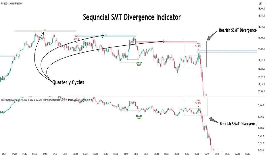
ICT Judas + Silver Bullet🔰 ICT Judas + Silver Bullet Indicator (SMC-based)
Built for Prop Firm and High Win Rate Intraday Traders
This indicator identifies key institutional setups from Inner Circle Trader (ICT) and Smart Money Concepts (SMC) strategies, optimized for XAUUSD, EURUSD, and other high-volume pairs on the 5-minute chart.
📌 Core Features:
✅ Asian Range Box (02:00–08:00 SGT) – used as manipulation anchor
✅ London Killzone (14:00–16:00 SGT) – Judas Swing detection
✅ New York Killzone (22:30–23:30 SGT) – Silver Bullet setups
✅ Automatic Fair Value Gap (FVG) detection
✅ Liquidity sweep detection based on 20-bar EQH/EQL
✅ Entry + Stop Loss + Take Profit visualization with adjustable RR
✅ Alerts for Judas and Silver setups
✅ Perfect for prop firm scalping and intraday swing logic
🛠️ How It Works:
- Judas Swing: triggers when liquidity above the Asian high is swept during London Killzone
- Silver Bullet: triggers when liquidity below recent lows is swept during NY Killzone
- Entry shown via circle, SL and TP lines based on user-defined RR and stop-loss pip distance
- Designed to be paired with SMC/ICT OB/FVG confirmation entries
⚙️ Settings:
- Adjustable session times
- Toggle FVG display
- Set RR and SL pips to match prop firm rules
- Compatible with alert webhooks for Telegram
🕰️ Note:
All times are fixed to **SGT (GMT+8)**. If you're in another timezone, adjust your TradingView timezone accordingly or update the session inputs manually during Daylight Saving Time changes.
🔔 Alert-Ready:
Use alerts for live signals and pair with webhooks for automation.
🔍 Recommended Pairings:
XAUUSD, EURUSD, GBPUSD, NAS100 on M5 chart
📈 Win Rate Potential:
Backtested with high-probability setups aligned with prop firm daily goals. Best used with strict discipline and 1-2 setups per day.
—
Built with ❤️ by a trader, for traders looking for precision-based executions using ICT logic.
RSI Support & Resistance Breakouts with OrderblocksThis tool is an overly simplified method of finding market squeeze and breakout completely based on a dynamic RSI calculation. It is designed to draw out areas of price levels where the market is pushing back against price action leaving behind instances of short term support and resistance levels you otherwise wouldn't see with the common RSI.
It uses the changes in market momentum to determine support and resistance levels in real time while offering price zone where order blocks exist in the short term.
In ranging markets we need to know a couple things.
1. External Zone - It's important to know where the highs and lows were left behind as they hold liquidity. Here you will have later price swings and more false breakouts.
2. Internal Zone - It's important to know where the highest and lowest closing values were so we can see the limitations of that squeeze. Here you will find the stronger cluster of orders often seen as orderblocks.
In this tool I've added a 200 period Smoothed Moving Average as a trend filter which causes the RSI calculation to change dynamically.
Regular Zones - without extending
The Zones draw out automatically but are often too small to work with.
To solve this problem, you can extend the zones into the future up to 40 bars.
This allows for more visibility against future price action.
--------------------------------------------
Two Types of Zones
External Zones - These zones give you positioning of the highest and lowest price traded within the ranging market. This is where liquidity will be swept and often is an ultimate breaking point for new price swings.
How to use them :
External Zones - External zones form at the top of a pullback. After this price should move back into its impulsive wave.
During the next corrective way, if price breaches the top of the previous External Zone, this is a sign of trend weakness. Expect a divergence and trend reversal.
Internal Zones - (OrderBlocks) Current price will move in relation to previous internal zones. The internal zone is where a majority of price action and trading took place. It's a stronger SQUEEZE area. Current price action will often have a hard time closing beyond the previous Internal Zones high or low. You can expect these zones to show you where the market will flip over. In these same internal zones you'll find large rejection candles.
**Important Note** Size Doesn't Matter
The size of the internal zone does not matter. It can be very small and still very powerful.
Once an internal zone has been hit a few times, its often not relevant any longer.
Order Block Zone Examples
In this image you can see the Internal Zone that was untouched had a STRONG price reaction later on.
Internal Zones that were touched multiple times had weak reactions later as price respected them less over time.
Zone Overlay Breakdown
The Zones form and update in real time until momentum has picked up and price begins to trend. However it leaves behind the elements of the inducement area and all the key levels you need to know about for future price action.
Resistance Fakeout : Later on after the zone has formed, price will return to this upper zone of price levels and cause fakeouts. A close above this zone implies the market moves long again.
Midline Equilibrium : This is simply the center of the strongest traded area. We can call this the Point of Control within the orderblock. If price expands through both extremes of this zone multiple times in the future, it eliminates the orderblock.
Support Fakeout : Just like its opposing brother, price will wick through this zone and rip back causing inducement to trap traders. You would need a clear close below this zone to be in a bearish trend.
BARCOLOR or Candle Color: (Optional)
Bars are colored under three conditions
Bullish Color = A confirmed bullish breakout of the range.
Bearish Color = A confirmed bearish breakout of the range.
Squeeze Color = Even if no box is formed a candle or candles can have a squeeze color. This means the ranging market happened within the high and low of that singular candle.
StatPivot- Dynamic Range Analyzer - indicator [PresentTrading]Hello everyone! In the following few open scripts, I would like to share various statistical tools that benefit trading. For this time, it is a powerful indicator called StatPivot- Dynamic Range Analyzer that brings a whole new dimension to your technical analysis toolkit.
This tool goes beyond traditional pivot point analysis by providing comprehensive statistical insights about price movements, helping you identify high-probability trading opportunities based on historical data patterns rather than subjective interpretations. Whether you're a day trader, swing trader, or position trader, StatPivot's real-time percentile rankings give you a statistical edge in understanding exactly where current price action stands within historical contexts.
Welcome to share your opinions! Looking forward to sharing the next tool soon!
█ Introduction and How it is Different
StatPivot is an advanced technical analysis tool that revolutionizes retracement analysis. Unlike traditional pivot indicators that only show static support/resistance levels, StatPivot delivers dynamic statistical insights based on historical pivot patterns.
Its key innovation is real-time percentile calculation - while conventional tools require new pivot formations before updating (often too late for trading decisions), StatPivot continuously analyzes where current price stands within historical retracement distributions.
Furthermore, StatPivot provides comprehensive statistical metrics including mean, median, standard deviation, and percentile distributions of price movements, giving traders a probabilistic edge by revealing which price levels represent statistically significant zones for potential reversals or continuations. By transforming raw price data into statistical insights, StatPivot helps traders move beyond subjective price analysis to evidence-based decision making.
█ Strategy, How it Works: Detailed Explanation
🔶 Pivot Point Detection and Analysis
The core of StatPivot's functionality begins with identifying significant pivot points in the price structure. Using the parameters left and right, the indicator locates pivot highs and lows by examining a specified number of bars to the left and right of each potential pivot point:
Copyp_low = ta.pivotlow(low, left, right)
p_high = ta.pivothigh(high, left, right)
For a point to qualify as a pivot low, it must have left higher lows to its left and right higher lows to its right. Similarly, a pivot high must have left lower highs to its left and right lower highs to its right. This approach ensures that only significant turning points are recognized.
🔶 Percentage Change Calculation
Once pivot points are identified, StatPivot calculates the percentage changes between consecutive pivot points:
For drops (when a pivot low is lower than the previous pivot low):
CopydropPercent = (previous_pivot_low - current_pivot_low) / previous_pivot_low * 100
For rises (when a pivot high is higher than the previous pivot high):
CopyrisePercent = (current_pivot_high - previous_pivot_high) / previous_pivot_high * 100
These calculations quantify the magnitude of each market swing, allowing for statistical analysis of historical price movements.
🔶 Statistical Distribution Analysis
StatPivot computes comprehensive statistics on the historical distribution of drops and rises:
Average (Mean): The arithmetic mean of all recorded percentage changes
CopyavgDrop = array.avg(dropValues)
Median: The middle value when all percentage changes are arranged in order
CopymedianDrop = array.median(dropValues)
Standard Deviation: Measures the dispersion of percentage changes from the average
CopystdDevDrop = array.stdev(dropValues)
Percentiles (25th, 75th): Values below which 25% and 75% of observations fall
Copyq1 = array.get(sorted, math.floor(cnt * 0.25))
q3 = array.get(sorted, math.floor(cnt * 0.75))
VaR95: The maximum expected percentage drop with 95% confidence
Copyvar95D = array.get(sortedD, math.floor(nD * 0.95))
Coefficient of Variation (CV): Measures relative variability
CopycvD = stdDevDrop / avgDrop
These statistics provide a comprehensive view of market behavior, enabling traders to understand the typical ranges and extreme moves.
🔶 Real-time Percentile Ranking
StatPivot's most innovative feature is its real-time percentile calculation. For each current price, it calculates:
The percentage drop from the latest pivot high:
CopycurrentDropPct = (latestPivotHigh - close) / latestPivotHigh * 100
The percentage rise from the latest pivot low:
CopycurrentRisePct = (close - latestPivotLow) / latestPivotLow * 100
The percentile ranks of these values within the historical distribution:
CopyrealtimeDropRank = (count of historical drops <= currentDropPct) / total drops * 100
This calculation reveals exactly where the current price movement stands in relation to all historical movements, providing crucial context for decision-making.
🔶 Cluster Analysis
To identify the most common retracement zones, StatPivot performs a cluster analysis by dividing the range of historical drops into five equal intervals:
CopyrangeSize = maxVal - minVal
For each interval boundary:
Copyboundaries = minVal + rangeSize * i / 5
By counting the number of observations in each interval, the indicator identifies the most frequently occurring retracement zones, which often serve as significant support or resistance areas.
🔶 Expected Price Targets
Using the statistical data, StatPivot calculates expected price targets:
CopytargetBuyPrice = close * (1 - avgDrop / 100)
targetSellPrice = close * (1 + avgRise / 100)
These targets represent statistically probable price levels for potential entries and exits based on the average historical behavior of the market.
█ Trade Direction
StatPivot functions as an analytical tool rather than a direct trading signal generator, providing statistical insights that can be applied to various trading strategies. However, the data it generates can be interpreted for different trade directions:
For Long Trades:
Entry considerations: Look for price drops that reach the 70-80th percentile range in the historical distribution, suggesting a statistically significant retracement
Target setting: Use the Expected Sell price or consider the average rise percentage as a reasonable target
Risk management: Set stop losses below recent pivot lows or at a distance related to the statistical volatility (standard deviation)
For Short Trades:
Entry considerations: Look for price rises that reach the 70-80th percentile range, indicating an unusual extension
Target setting: Use the Expected Buy price or average drop percentage as a target
Risk management: Set stop losses above recent pivot highs or based on statistical measures of volatility
For Range Trading:
Use the most common drop and rise clusters to identify probable reversal zones
Trade bounces between these statistically significant levels
For Trend Following:
Confirm trend strength by analyzing consecutive higher pivot lows (uptrend) or lower pivot highs (downtrend)
Use lower percentile retracements (20-30th percentile) as entry opportunities in established trends
█ Usage
StatPivot offers multiple ways to integrate its statistical insights into your trading workflow:
Statistical Table Analysis: Review the comprehensive statistics displayed in the data table to understand the market's behavior. Pay particular attention to:
Average drop and rise percentages to set reasonable expectations
Standard deviation to gauge volatility
VaR95 for risk assessment
Real-time Percentile Monitoring: Watch the real-time percentile display to see where the current price movement stands within the historical distribution. This can help identify:
Extreme movements (90th+ percentile) that might indicate reversal opportunities
Typical retracements (40-60th percentile) that might continue further
Shallow pullbacks (10-30th percentile) that might represent continuation opportunities in trends
Support and Resistance Identification: Utilize the plotted pivot points as key support and resistance levels, especially when they align with statistically significant percentile ranges.
Target Price Setting: Use the expected buy and sell prices calculated from historical averages as initial targets for your trades.
Risk Management: Apply the statistical measurements like standard deviation and VaR95 to set appropriate stop loss levels that account for the market's historical volatility.
Pattern Recognition: Over time, learn to recognize when certain percentile levels consistently lead to reversals or continuations in your specific market, and develop personalized strategies based on these observations.
█ Default Settings
The default settings of StatPivot have been carefully calibrated to provide reliable statistical analysis across a variety of markets and timeframes, but understanding their effects allows for optimal customization:
Left Bars (30) and Right Bars (30): These parameters determine how pivot points are identified. With both set to 30 by default:
A pivot low must be the lowest point among 30 bars to its left and 30 bars to its right
A pivot high must be the highest point among 30 bars to its left and 30 bars to its right
Effect on performance: Larger values create fewer but more significant pivot points, reducing noise but potentially missing important market structures. Smaller values generate more pivot points, capturing more nuanced movements but potentially including noise.
Table Position (Top Right): Determines where the statistical data table appears on the chart.
Effect on performance: No impact on analytical performance, purely a visual preference.
Show Distribution Histogram (False): Controls whether the distribution histogram of drop percentages is displayed.
Effect on performance: Enabling this provides visual insight into the distribution of retracements but can clutter the chart.
Show Real-time Percentile (True): Toggles the display of real-time percentile rankings.
Effect on performance: A critical setting that enables the dynamic analysis of current price movements. Disabling this removes one of the key advantages of the indicator.
Real-time Percentile Display Mode (Label): Chooses between label display or indicator line for percentile rankings.
Effect on performance: Labels provide precise information at the current price point, while indicator lines show the evolution of percentile rankings over time.
Advanced Considerations for Settings Optimization:
Timeframe Adjustment: Higher timeframes generally benefit from larger Left/Right values to identify truly significant pivots, while lower timeframes may require smaller values to capture shorter-term swings.
Volatility-Based Tuning: In highly volatile markets, consider increasing the Left/Right values to filter out noise. In less volatile conditions, lower values can help identify more potential entry and exit points.
Market-Specific Optimization: Different markets (forex, stocks, commodities) display different retracement patterns. Monitor the statistics table to see if your market typically shows larger or smaller retracements than the current settings are optimized for.
Trading Style Alignment: Adjust the settings to match your trading timeframe. Day traders might prefer settings that identify shorter-term pivots (smaller Left/Right values), while swing traders benefit from more significant pivots (larger Left/Right values).
By understanding how these settings affect the analysis and customizing them to your specific market and trading style, you can maximize the effectiveness of StatPivot as a powerful statistical tool for identifying high-probability trading opportunities.