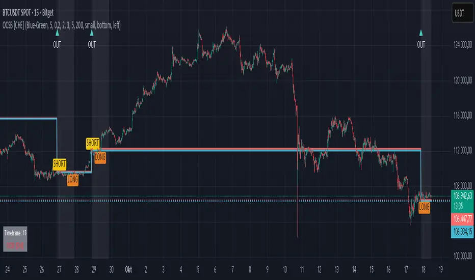
Outside Candle Session Breakout [CHE]Outside Candle Session Breakout
Session - anchored HTF levels for clear market-structure and precise breakout context
Summary
This indicator is a relevant market-structure tool. It anchors the session to the first higher-timeframe bar, then activates only when the second bar forms an outside condition. Price frequently reacts around these anchors, which provides precise breakout context and a clear overview on both lower and higher timeframes. Robustness comes from close-based validation, an adaptive volatility and tick buffer, first-touch enforcement, optional retest, one-signal-per-session, cooldown, and an optional trend filter.
Pine version: v6. Overlay: true.
Motivation: Why this design?
Short-term breakout tools often trigger during noise, duplicate within the same session, or drift when volatility shifts. The core idea is to gate signals behind a meaningful structure event: a first-bar anchor and a subsequent outside bar on the session timeframe. This narrows attention to structurally important breaks while adaptive buffering and debouncing reduce false or mid-run triggers.
What’s different vs. standard approaches?
Baseline: Simple high-low breaks or fixed buffers without session context.
Architecture: Session-anchored first-bar high/low; outside-bar gate; close-based confirmation with an adaptive ATR and tick buffer; first-touch enforcement; optional retest window; one-signal-per-session and cooldown; optional EMA trend and slope filter; higher-timeframe aggregation with lookahead disabled; themeable visuals and a range fill between levels.
Practical effect: Cleaner timing at structurally relevant levels, fewer redundant or late triggers, and better multi-timeframe situational awareness.
How it works (technical)
The chart timeframe is mapped to an analysis timeframe and a session timeframe.
The first session bar defines the anchor high and low. The setup becomes active only after the next bar forms an outside range relative to that first bar.
While active, the script tracks these anchors and checks for a breakout beyond a buffered threshold, using closing prices or wicks by preference.
The buffer scales with volatility and is limited by a minimum tick floor. First-touch enforcement avoids mid-run confirmations.
Optional retest requires a pullback to the raw anchor followed by a new close beyond the buffered level within a user window.
Optional trend gating uses an EMA on the analysis timeframe, including an optional slope requirement and price-location check.
Higher-timeframe data is requested with lookahead disabled. Values can update during a forming higher-timeframe bar; waiting and confirmation mitigate timing shifts.
Parameter Guide
Enable Long / Enable Short — Direction toggles. Default: true / true. Reduces unwanted side.
Wait Candles — Minimum bars after outside confirmation before entries. Default: five. More waiting increases stability.
Close-based Breakout — Confirm on candle close beyond buffer. Default: true. For wick sensitivity, disable.
ATR Buffer — Enables adaptive volatility buffer. Default: true.
ATR Multiplier — Buffer scaling. Default: zero point two. Increase to reduce noise.
Ticks Buffer — Minimum buffer in ticks. Default: two. Protects in quiet markets.
Cooldown Bars — Blocks new signals after a trigger. Default: three.
One Signal per Session — Prevents duplicates within a session. Default: true.
Require Retest — Pullback to raw anchor before confirming. Default: false.
Retest Window — Bars allowed for retest completion. Default: five.
HTF Trend Filter — EMA-based gating. Default: false.
EMA Length — EMA period. Default: two hundred.
Slope — Require EMA slope direction. Default: true.
Price Above/Below EMA — Require price location relative to EMA. Default: true.
Show Levels / Highlight Session / Show Signals — Visual controls. Default: true.
Color Theme — “Blue-Green” (default), “Monochrome”, “Earth Tones”, “Classic”, “Dark”.
Time Period Box — Visibility, size, position, and colors for the info box. (Optional)
Reading & Interpretation
The two level lines represent the session’s first-bar high and low. The filled band illustrates the active session range.
“OUT” marks that the outside condition is confirmed and the setup is live.
“LONG” or “SHORT” appears only when the breakout clears buffer, debounce, and optional gates.
Background tint indicates sessions where the setup is valid.
Alerts fire on confirmed long or short breakout events.
Practical Workflows & Combinations
Trend-following: Keep close-based validation, ATR buffer near the default, one-signal-per-session enabled; add EMA trend and slope for directional bias.
Retest confirmation: Enable retest with a short window to prioritize cleaner continuation after a pullback.
Lower-timeframe scalping: Reduce waiting and cooldown slightly; keep a small tick buffer to filter micro-whips.
Swing and position context: Increase ATR multiplier and waiting; maintain once-per-session to limit duplicates.
Timeframe Tiers and Trader Profiles
The script adapts its internal mapping based on the chart timeframe:
Under fifteen minutes → Analysis: one minute; Session: sixty minutes. Useful for scalpers and high-frequency intraday reads.
Between fifteen and under sixty minutes → Analysis: fifteen minutes; Session: one day. Suits day traders who need intraday alignment to the daily session.
Between sixty minutes and under one day → Analysis: sixty minutes; Session: one week. Serves intraday-to-swing transitions and end-of-day planning.
Between one day and under one week → Analysis: two hundred forty minutes; Session: two weeks. Fits swing traders who monitor multi-day structure.
Between one week and under thirty days → Analysis: one day; Session: three months. Supports position traders seeking quarterly context.
Thirty days and above → Analysis: one day; Session: twelve months. Provides a broad annual anchor for macro context.
These tiers are designed to keep anchors meaningful across regimes while preserving responsiveness appropriate to the trader profile.
Behavior, Constraints & Performance
Signals can be validated on closed bars through close-based logic; enabling this reduces intrabar flicker.
Higher-timeframe values may evolve during a forming bar; waiting parameters and the outside-bar gate reduce, but do not remove, this effect.
Resource footprint is light; the script uses standard indicators and a single higher-timeframe request per stream.
Known limits: rare setups during very quiet periods, sensitivity to gaps, and reduced reliability on illiquid symbols.
Sensible Defaults & Quick Tuning
Start with close-based validation on, ATR buffer on with a multiplier near zero point two, tick buffer two, cooldown three, once-per-session on.
Too many flips: increase the ATR multiplier and cooldown; consider enabling the EMA filter and slope.
Too sluggish: reduce the ATR multiplier and waiting; disable retest.
Choppy conditions: keep close-based validation, increase tick buffer, shorten the retest window.
What this indicator is—and isn’t
This is a visualization and signal layer for session-anchored breakouts with stability gates. It is not a complete trading system, risk framework, or predictive engine. Combine it with structured analysis, position sizing, and disciplined risk controls.
Disclaimer
The content provided, including all code and materials, is strictly for educational and informational purposes only. It is not intended as, and should not be interpreted as, financial advice, a recommendation to buy or sell any financial instrument, or an offer of any financial product or service. All strategies, tools, and examples discussed are provided for illustrative purposes to demonstrate coding techniques and the functionality of Pine Script within a trading context.
Any results from strategies or tools provided are hypothetical, and past performance is not indicative of future results. Trading and investing involve high risk, including the potential loss of principal, and may not be suitable for all individuals. Before making any trading decisions, please consult with a qualified financial professional to understand the risks involved.
By using this script, you acknowledge and agree that any trading decisions are made solely at your discretion and risk.
Do not use this indicator on Heikin-Ashi, Renko, Kagi, Point-and-Figure, or Range charts, as these chart types can produce unrealistic results for signal markers and alerts.
Best regards and happy trading
Chervolino
"scalping" için komut dosyalarını ara
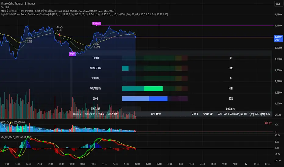
Digital RPM HUD — 4 Feeds + Confidence + Timeline (v3)🏎️ Digital RPM HUD — 4 Feeds + Confidence + Timeline (v3)
A performance-style trading dashboard for momentum-driven traders.
The Digital RPM HUD gives you an instant visual readout of market “engine speed” — combining four customizable data feeds (Trend, Momentum, Volume, Volatility) into a single confidence score (0–100) and a color-coded timeline of regime changes.
Think of it as a racing-inspired control panel: you only “hit the throttle” when confidence is high and all systems agree.
🔧 Key Features
4 Data Feeds – assign your own logic (EMA, RSI, RVOL, ATR, etc.).
Confidence Meter – blends the four feeds into one smooth 0–100 reading.
Timeline Strip – shows recent bullish / bearish / neutral states at a glance.
Visual Trade Cues – optional on-chart LONG / SHORT / EXIT markers.
Fully Customizable – thresholds, weights, smoothing, colors, layout.
HUD Overlay – clean, minimal, and adjustable to any corner of your chart.
💡 How to Use
Configure each feed to reflect your preferred signals (e.g., trend EMA 200, momentum RSI 14, volume RVOL 20, volatility ATR 14).
Watch the Confidence gauge:
✅ Above Bull Threshold → Market acceleration / long bias.
❌ Below Bear Threshold → Momentum loss / short bias.
⚪ Between thresholds → Neutral zone; stay patient.
Use the Timeline to confirm trend consistency — more green = bullish regime, more red = bearish.
⚙️ Recommended Setups
Scalping: Trend EMA 50 + RSI 7 + RVOL 10 + ATR 7 → Fast response.
Intraday: EMA 200 + RSI 14 + RVOL 20 + ATR 14 → Balanced signal.
Swing: Multi-TF Trend + MACD + RVOL + ATR → Smooth and steady.
⚠️ Disclaimer
This script is not a trading strategy and does not execute trades.
All signals are visual aids — always confirm with your own analysis and risk management.
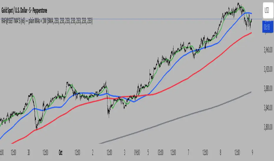
RAF@SSET POWER-7 MA SuiteWhat it is
A clean, lightweight pack of seven moving averages (1m, 5m, 15m, 1H, 4H, 1D, 1W).
HTF lines are confirmed-only (no intra-bar wiggle), so what you see is what closed—no repaint on HTFs. Use it to anchor scalps to higher-timeframe structure without clutter.
Why you’ll like it
1m→1W in one look – see alignment from scalp to swing.
Confirmed HTFs – uses request.security() with lookahead_off and only plots closed values.
Zero fluff – just MAs, fixed colors, ultra-fast.
Your presets – default to my “Power-7” lengths (e.g., 233) or set your own.
SMA/EMA switch – pick your poison globally.
Inputs
Show/hide: 1m, 5m, 15m, 1H, 4H, 1D, 1W
Length per TF (defaults 233)
MA type: SMA / EMA
Color per TF
How it works (short)
Current-TF MA updates live.
Higher TF MAs (5m, 15m, 1H, 4H/“240”, 1D, 1W) only update when their candle closes. That removes “wiggle” and surprise shifts.
Tips
For scalping: trade off LTF, bias from 1H/4H/1D.
For swing: let 1D/1W set bias; use 1H/4H for timing.
Your current chart TF MA is live (by design). If you want it confirmed too, set your chart to the HTF you care about.
Built from my RAF@SSET workflow. Shoutout to everyone who keeps indicators simple and readable.
v1.0: First public release (Pine v6). Seven MAs (1m→1W), confirmed HTFs, fixed colors, SMA/EMA toggle.
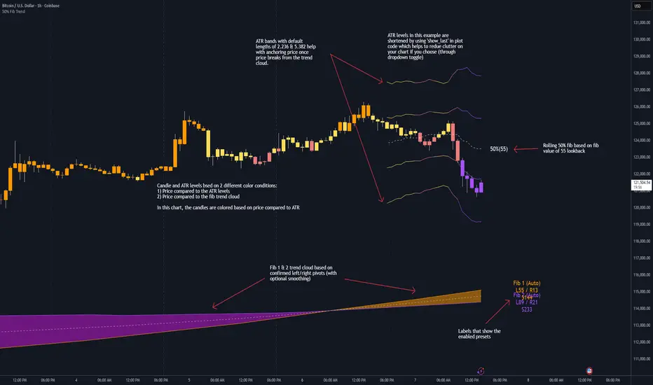
50% Fib Trend Cloud + ATR BandsThis indicator plots two structural 50% fibonacci midpoints from recent confirmed 'left/right' swings that form a *cloud* of equilibrium, then adds a rolling 50% fibonacci range midpoint based on a lookback window that's wrapped in ATR bands. Importantly, it solves a specific trading problem:
Structural midpoints (macro context) are powerful but can lag when price escapes prior ranges. Enter rolling 50% fib + ATR ➡️ which restores real-time balance & tolerance (micro context). Together they show where price is balanced structurally, where it’s balanced right now, and how much volatility to tolerate before acting.
➖➖➖
🔑 Why this is different
Most tools either draw a single midpoint (ex., daily 50%) or ATR bands around a moving average. This script fuses dual swing-based 50% midpoints (structure) + a rolling 50% with ATR (flow), so you don’t lose context when price escapes prior ranges. The cloud tells you who’s in control (fast vs. slow structure). The rolling 50% + ATR tells you how far is “too far” now.
➖➖➖
🧠 What it does (at a glance)
🔸Structural Equilibrium × 2 (Fib1/Fib2)
Two independent 50% midpoints formed from swing pivots (configurable Left/Right bars + optional smoothing). Their gap is the Midpoint Cloud = structural “fair value” zone.
🔸Rolling 50% + ATR Bands
A rolling highest/lowest window computes an always-current 50% rolling midpoint plot; ±ATR × length envelopes define a soft value area and over-stretch boundaries.
🔸Actionable Visuals
Optional fill between Fib1/Fib2, labels, and candle-overlay modes to instantly read regime (above both / below both / between).
🔸Smart Defaults
Timeframe-aware presets for L/R pivots & smoothing; full manual overrides available.
➖➖➖
⚙️ Calculations (plain-English)
🔸Pivot midpoints (Fib1 & Fib2):
1) Detect a swing using `Left/Right` bars
2) Take the swing’s high/low → compute 50%
3) (Optional) Smooth the line (SMA) to stabilize on noisy TFs
4) Repeat with a different sensitivity to get two distinct midpoints
🔸Rolling midpoint:
Highest High / Lowest Low over the last *N* bars → (HH + LL) / 2
🔸ATR levels:
`Upper = Rolling50 + ATR × Mult`, `Lower = Rolling50 − ATR × Mult`
(Typical: ATR length 14–21; Multipliers 2.236 for L1, 5.382 for L2)
➖➖➖
🤖 Auto-Configured Presets (with Manual Override)
💡Goal: make the midpoints “just work” on common timeframes while still letting you dial them in.
💡How Auto Presets work
When Auto Presets = ON, the script picks sensible L/R/S (Left bars / Right bars / Smoothing) for Fib Trend 1 and Fib Trend 2 based on chart timeframe.
🔸Fib 1 (fast) emphasizes *micro-structure* for quicker bias shifts.
🔸Fib 2 (slow) emphasizes *macro-structure* for anchor/bias context.
These defaults keep Fib 1 responsive without jitter and Fib 2 stable without lag.
➡️ Turn Auto Presets = OFF to take full control with the manual inputs described below.
➖➖➖
🛠 Manual Fib Midpoint Settings (when Auto = OFF)
💡Each midpoint uses three knobs:
🔸Pivot Left (L): bars to the left that must be lower/higher to qualify a swing
🔸Pivot Right (R): bars to the right that must be lower/higher to confirm the swing
🔸Smoothing (S): SMA period applied to the raw 50% midpoint (stabilizes noise)
5-Minute optimized defaults
🔸Fib Trend 1: `L21 / R5 / S55` → responsive local structure (entries/exits, re-balancing zones)
🔸Fib Trend 2: `L55 / R13 / S89` → broader structure (trend context, anchors/stops)
Timeframe guidance
🔸1m–3m: may feel a touch laggy → consider ~`L13 / R3 / S34`
🔸15m–1h: defaults remain strong → optionally ~`L34 / R8 / S89`
🔸4h+ : increase span for stability → `L89–144 / R13–21 / S144–233`
➡️ Rule of thumb: shorter L/R = faster detection, longer S = smoother line. Tune until Fib 1 captures the “active swing” and Fib 2 captures the “dominant swing” without whipsaw.
➖➖➖
🎛 Inputs (quick reference)
🔸Fib Trend 1/2: Source (High/Low/Close), Left/Right bars, Smoothing length, Show/Hide, Cloud fill toggle
🔸Rolling 50%: Lookback length, Price basis (Wicks/Close/HLC3/OHLC4), Plot scope (Full / Last N / None)
🔸ATR Bands: ATR length, Multipliers (L1/L2), Plot scope, Line width/colors
🔸Overlay & Labels: Candle overlay mode, Label padding/size, 50% centerline toggle, Plot widths
➖➖➖
🖍️ Candle Coloring & Overlay Modes
💡Purpose: make trend instantly visible on the candles and ATR levels.
1) Color Logic (dropdown)
🔸 Fib Midpoints — Colors by position of price vs. Fib 1 & Fib 2
🔸ATR Zones — Colors by which ATR zone price is in relative to the Rolling 50%
➡️ Price Reference: Choose the input used for the decision (Close, HL2, OHLC3, OHLC4).
➡️Tip: Close is crisp; HL2/OHLC variants are smoother.
2) Overlay Style (dropdown)
🔸 None — No visual change to candles
🔸 Bar Color — Uses `barcolor()` to tint built-in candles (this takes into account your Trading View settings, for instance if you have wicks set to white, they will show up as white with this setting)
🔸 PlotCandles — Draws unified custom candles (body, wick, border) with the same color for maximum clarity
💡Practical use
🔸 Pick Fib Midpoints to read structural bias at a glance (above/below/between the cloud).
🔸 Pick ATR Zones to read value vs. stretch around the Rolling 50% (mean-reversion vs. trend extension).
➖➖➖
📘 How to use
A) Trend confirmation
- Strong bullish bias when price holds above both structural mids; strong bearish when below both.
- Use the Rolling 50% + ATR as a dynamic re-entry zone: pullbacks that respect ATR(L1) often continue the prevailing trend.
B) Transition / mean reversion
- Inside the Cloud (between Fib1 & Fib2) treat behavior as neutralization/re-balancing; range tactics tend to outperform momentum plays.
- In ranges, fades near ±ATR around the rolling 50% can mark short-term edges.
C) Breakout context
- When price leaves the Cloud, the Rolling 50% keeps you anchored so price never feels “floating.” A clean hold outside ATR(L1/L2) suggests regime strength; quick re-entries hint at traps.
➖➖➖
🖼 Chart examples
➡️ Each snapshot shows how the Cloud (structure) and the Rolling 50% + ATR (flow) work together.
1) 1-Minute Downtrend – Cloud as Dynamic Ceiling
- The Cloud slopes down; pullbacks repeatedly fail under the Cloud’s underside.
- Rolling 50% (dashed mid) + ATR(L1) act as a reversion band: rallies stall near upper ATR and rotate lower.
2) 15-Minute Persistent Drift – Structure Guides, Flow Times Entries
- Long drift lower with Cloud overhead.
- Consolidations near the rolling mid resolve in the trend direction; ATR bands frame risk on each attempt.
3) 15-Minute Uptrend (BTC) – From Cloud Escape to Value Stair-Step
- After escaping the prior Cloud, rolling 50% + ATR establish a new higher value area.
- Pullbacks into ATR(L1) produce orderly stair-steps; Cloud remains supportive on deeper dips
4) 5-Minute BTC – Pullback to Value then Rotate
- Strong leg up; retrace tags lower ATR band and rotates back toward the rolling mid.
- Labels (Fib1/Fib2) make the structural context explicit for decision-making.
➖➖➖
🧪 Starter presets
- Intraday (5–15m): Fib1 ~ L21/R5 (smooth 5), Fib2 ~ L55/R13 (smooth 9) • Rolling = 55 • ATR = 14 • L1 = 2.5x, L2 = 5.0x
- Scalping: Shorten lookbacks & smoothing; keep ATR multipliers similar, or tighten L1.
- Swing: Lengthen all lookbacks; consider ATR length 21–28.
➖➖➖
🏁Final Word
This script is not just a visual tool, it’s a complete trend and structure framework. Whether you're looking for clean trend alignment, dynamic support/resistance, or early warning signs of a reversal, this system is tuned to help you react with confidence — not hindsight.
Rembember, no single indicator should be used in isolation. For best results, combine it with price action analysis, higher-timeframe context, and complementary tools like trendlines, moving averages etc Use it as part of a well-rounded trading approach to confirm setups — not to define them alone.
---
💡Turn logic into clarity. Structure into trades. And uncertainty into confidence.
Trend Fib Zone Bounce (TFZB) [KedArc Quant]Description:
Trend Fib Zone Bounce (TFZB) trades with the latest confirmed Supply/Demand zone using a single, configurable Fib pullback (0.3/0.5/0.6). Trade only in the direction of the most recent zone and use a single, configurable fib level for pullback entries.
• Detects market structure via confirmed swing highs/lows using a rolling window.
• Draws Supply/Demand zones (bearish/bullish rectangles) from the latest MSS (CHOCH or BOS) event.
• Computes intra zone Fib guide rails and keeps them extended in real time.
• Triggers BUY only inside bullish zones and SELL only inside bearish zones when price touches the selected fib and closes back beyond it (bounce confirmation).
• Optional labels print BULL/BEAR + fib next to the triangle markers.
What it does
Finds structure using confirmed swing highs/lows (you choose the confirmation length).
Builds the latest zone (bullish = demand, bearish = supply) after a CHOCH/BOS event.
Draws intra-zone “guide rails” (Fib lines) and extends them live.
Signals only with the trend of that zone:
BUY inside a bullish zone when price tags the selected Fib and closes back above it.
SELL inside a bearish zone when price tags the selected Fib and closes back below it.
Optional labels print BULL/BEAR + Fib next to triangles for quick context
Why this is different
Most “zone + fib + signal” tools bolt together several indicators, or fire counter-trend signals because they don’t fully respect structure. TFZB is intentionally minimal:
Single bias source: the latest confirmed zone defines direction; nothing else overrides it.
Single entry rule: one Fib bounce (0.3/0.5/0.6 selectable) inside that zone—no counter-trend trades by design.
Clean visuals: you can show only the most recent zone, clamp overlap, and keep just the rails that matter.
Deterministic & transparent: every plot/label comes from the code you see—no external series or hidden smoothing
How it helps traders
Cuts decision noise: you always know the bias and the only entry that matters right now.
Forces discipline: if price isn’t inside the active zone, you don’t trade.
Adapts to volatility: pick 0.3 in strong trends, 0.5 as the default, 0.6 in chop.
Non-repainting zones: swings are confirmed after Structure Length bars, then used to build zones that extend forward (they don’t “teleport” later)
How it works (details)
*Structure confirmation
A swing high/low is only confirmed after Structure Length bars have elapsed; the dot is plotted back on the original bar using offset. Expect a confirmation delay of about Structure Length × timeframe.
*Zone creation
After a CHOCH/BOS (momentum shift / break of prior swing), TFZB draws the new Supply/Demand zone from the swing anchors and sets it active.
*Fib guide rails
Inside the active zone TFZB projects up to five Fib lines (defaults: 0.3 / 0.5 / 0.7) and extends them as time passes.
*Entry logic (with-trend only)
BUY: bar’s low ≤ fib and close > fib inside a bullish zone.
SELL: bar’s high ≥ fib and close < fib inside a bearish zone.
*Optionally restrict to one signal per zone to avoid over-trading.
(Optional) Aggressive confirm-bar entry
When do the swing dots print?
* The code confirms a swing only after `structureLen` bars have elapsed since that candidate high/low.
* On a 5-min chart with `structureLen = 10`, that’s about 50 minutes later.
* When the swing confirms, the script plots the dot back on the original bar (via `offset = -structureLen`). So you *see* the dot on the old bar, but it only appears on the chart once the confirming bar arrives.
> Practical takeaway: expect swing markers to appear roughly `structureLen × timeframe` later. Zones and signals are built from those confirmed swings.
Best timeframe for this Indicator
Use the timeframe that matches your holding period and the noise level of the instrument:
* Intraday :
* 5m or 15m are the sweet spots.
* Suggested `structureLen`:
* 5m: 10–14 (confirmation delay \~50–70 min)
* 15m: 8–10 (confirmation delay \~2–2.5 hours)
* Keep Entry Fib at 0.5 to start; try 0.3 in strong trends, 0.6 in chop.
* Tip: avoid the first 10–15 minutes after the open; let the initial volatility set the early structure.
* Swing/overnight:
* 1h or 4h.
* `structureLen`:
* 1h: 6–10 (6–10 hours confirmation)
* 4h: 5–8 (20–32 hours confirmation)
* 1m scalping: not recommended here—the confirmation lag relative to the noise makes zones less reliable.
Inputs (all groups)
Structure
• Show Swing Points (structureTog)
o Plots small dots on the bar where a swing point is confirmed (offset back by Structure Length).
• Structure Length (structureLen)
o Lookback used to confirm swing highs/lows and determine local structure. Higher = fewer, stronger swings; lower = more reactive.
Zones
• Show Last (zoneDispNum)
o Maximum number of zones kept on the chart when Display All Zones is off.
• Display All Zones (dispAll)
o If on, ignores Show Last and keeps all zones/levels.
• Zone Display (zoneFilter): Bullish Only / Bearish Only / Both
o Filters which zone types are drawn and eligible for signals.
• Clean Up Level Overlap (noOverlap)
o Prevents fib lines from overlapping when a new zone starts near the previous one (clamps line start/end times for readability).
Fib Levels
Each row controls whether a fib is drawn and how it looks:
• Toggle (f1Tog…f5Tog): Show/hide a given fib line.
• Level (f1Lvl…f5Lvl): Numeric ratio in . Defaults active: 0.3, 0.5, 0.7 (0 and 1 off by default).
• Line Style (f1Style…f5Style): Solid / Dashed / Dotted.
• Bull/Bear Colors (f#BullColor, f#BearColor): Per-fib color in bullish vs bearish zones.
Style
• Structure Color: Dot color for confirmed swing points.
• Bullish Zone Color / Bearish Zone Color: Rectangle fills (transparent by default).
Signals
• Entry Fib for Signals (entryFibSel): Choose 0.3, 0.5 (default), or 0.6 as the trigger line.
• Show Buy/Sell Signals (showSignals): Toggles triangle markers on/off.
• One Signal Per Zone (oneSignalPerZone): If on, suppresses additional entries within the same zone after the first trigger.
• Show Signal Text Labels (Bull/Bear + Fib) (showSignalLabels): Adds a small label next to each triangle showing zone bias and the fib used (e.g., BULL 0.5 or BEAR 0.3).
How TFZB decides signals
With trend only:
• BUY
1. Latest active zone is bullish.
2. Current bar’s close is inside the zone (between top and bottom).
3. The bar’s low ≤ selected fib and it closes > selected fib (bounce).
• SELL
1. Latest active zone is bearish.
2. Current bar’s close is inside the zone.
3. The bar’s high ≥ selected fib and it closes < selected fib.
Markers & labels
• BUY: triangle up below the bar; optional label “BULL 0.x” above it.
• SELL: triangle down above the bar; optional label “BEAR 0.x” below it.
Right-Panel Swing Log (Table)
What it is
A compact, auto-updating log of the most recent Swing High/Low events, printed in the top-right of the chart.
It helps you see when a pivot formed, when it was confirmed, and at what price—so you know the earliest bar a zone-based signal could have appeared.
Columns
Type – Swing High or Swing Low.
Date – Calendar date of the swing bar (follows the chart’s timezone).
Swing @ – Time of the original swing bar (where the dot is drawn).
Confirm @ – Time of the bar that confirmed that swing (≈ Structure Length × timeframe after the swing). This is also the earliest moment a new zone/entry can be considered.
Price – The swing price (high for SH, low for SL).
Why it’s useful
Clarity on repaint/confirmation: shows the natural delay between a swing forming and being usable—no guessing.
Planning & journaling: quick reference of today’s pivots and prices for notes/backtesting.
Scanning intraday: glance to see if you already have a confirmed zone (and therefore valid fib-bounce entries), or if you’re still waiting.
Context for signals: if a fib-bounce triangle appears before the time listed in Confirm @, it’s not a valid trade (you were too early).
Settings (Inputs → Logging)
Log swing times / Show table – turn the table on/off.
Rows to keep – how many recent entries to display.
Show labels on swing bar – optional tags on the chart (“Swing High 11:45”, “Confirm SH 14:15”) that match the table.
Recommended defaults
• Structure Length: 10–20 for intraday; 20–40 for swing.
• Entry Fib for Signals: 0.5 to start; try 0.3 in stronger trends and 0.6 in choppier markets.
• One Signal Per Zone: ON (prevents over trading).
• Zone Display: Both.
• Fib Lines: Keep 0.3/0.5/0.7 on; turn on 0 and 1 only if you need anchors.
Alerts
Two alert conditions are available:
• BUY signal – fires when a with trend bullish bounce at the selected fib occurs inside a bullish zone.
• SELL signal – fires when a with trend bearish bounce at the selected fib occurs inside a bearish zone.
Create alerts from the chart’s Alerts panel and select the desired condition. Use Once Per Bar Close to avoid intrabar flicker.
Notes & tips
• Swing dots are confirmed only after Structure Length bars, so they plot back in time; zones built from these confirmed swings do not repaint (though they extend as new bars form).
• If you don’t see a BUY where you expect one, check: (1) Is the active zone bullish? (2) Did the candle’s low actually pierce the selected fib and close above it? (3) Is One Signal Per Zone suppressing a second entry?
• You can hide visual clutter by reducing Show Last to 1–3 while keeping Display All Zones off.
Glossary
• CHOCH (Change of Character): A shift where price breaks beyond the last opposite swing while local momentum flips.
• BOS (Break of Structure): A cleaner break beyond the prior swing level in the current momentum direction.
• MSS: Either CHOCH or BOS – any event that spawns a new zone.
Extension ideas (optional)
• Add fib extensions (1.272 / 1.618) for target lines.
• Zone quality score using ATR normalization to filter weak impulses.
• HTF filter to only accept zones aligned with a higher timeframe trend.
⚠️ Disclaimer This script is provided for educational purposes only.
Past performance does not guarantee future results.
Trading involves risk, and users should exercise caution and use proper risk management when applying this strategy.

VWAP Momentum Oscillator How It Works
Core Calculation Method
The oscillator combines four key market measurements into a single, normalized reading:
1. Price-VWAP Deviation: `(Close - VWAP) / VWAP × 100`
2. VWAP-MA Momentum: `(VWAP - MovingAverage) / MovingAverage × 100`
3. Anchored VWAP Strength: Average of high/low anchor deviations from rolling VWAP
4. Range Position: `(Close - PeriodLow) / (PeriodHigh - PeriodLow) × 100 - 50`
Dynamic Signal Line
The signal line uses an EMA that automatically adjusts its length based on your chart timeframe:
- Futures: Always covers 23 hours of trading (1,380 minutes)
- Stocks: Always covers 6.5 hours of trading (390 minutes)
- Examples: 276 periods on 5-min futures chart, 1,380 periods on 1-min futures chart
Trading Signals
🟢 Buy Signals
- Condition: Main oscillator crosses above signal line while below zero
- Logic: Momentum turning bullish from oversold conditions
- Visual: Green "BUY" label below price action
🔴 Sell Signals
- Condition: Main oscillator crosses below signal line while above zero
- Logic: Momentum turning bearish from overbought conditions
- Visual: Red "SELL" label above price action
⚠️ Extreme Warnings
- Extreme Overbought: Red triangle when oscillator crosses above +4.0
- Extreme Oversold: Green triangle when oscillator crosses below -4.0
- Purpose: Risk management alerts, not entry/exit signals
Oscillator Zones
Interpretation Guide
- Above +2.0: Strong bullish momentum zone (green background)
- 0 to +2.0: Mild bullish territory
- 0 to -2.0: Mild bearish territory
- Below -2.0: Strong bearish momentum zone (red background)
- Above +4.0: Extreme overbought (caution advised)
- Below -4.0: Extreme oversold (potential reversal zone)
Customization Options
Moving Average Settings
- EMA/SMA Toggle: Choose between exponential or simple moving average
- Color Customization: Adjust MA line color and width
Visual Controls
- Bullish/Bearish Colors: Customize momentum zone colors
- Signal Line: Toggle visibility and adjust color
- Line Widths: Control thickness of all plot lines
Anchor Modes
- NY Session Only: Anchors reset at NY market open (9:30 AM ET)
- 24H NY Day: Anchors reset at NY calendar day change (midnight ET)
Best Practices
Timeframe Selection
- Scalping: 1-5 minute charts for quick momentum changes
- Day Trading: 5-15 minute charts for clearer trend signals
- Swing Trading: 1-4 hour charts for major momentum shifts
Signal Confirmation
- Wait for crossovers: Don't trade on oscillator position alone
- Respect extreme levels: Exercise caution above +4 or below -4
- Use with price action: Combine with support/resistance levels
Risk Management
- Extreme zones: Reduce position size when oscillator is extended
- Failed signals: Exit quickly if momentum doesn't follow through
- Market context: Consider overall trend direction and market volatility
Technical Specifications
Calculation Components
- Base Length: 1,380 periods (futures) / 390 periods (stocks)
- Signal Line: Dynamic EMA covering one full trading day
- Smoothing: 3-period SMA on raw oscillator (adjustable)
- Update Frequency: Real-time on every price tick
Performance Notes
- Resource Efficient: Optimized calculations minimize CPU usage
- Memory Friendly: Uses incremental VWAP calculations
- Fast Loading: Minimal historical data requirements
Version History & Development
This oscillator evolved from advanced VWAP overlay strategies, transforming complex multi-line analysis into a single, actionable momentum gauge. The indicator maintains the sophistication of institutional VWAP analysis while providing the clarity needed for retail trading decisions.
Core Philosophy
Traditional VWAP indicators show where price is relative to volume-weighted averages, but they don't quantify momentum or provide clear entry/exit signals. This oscillator solves that problem by normalizing all VWAP relationships into a single, bounded indicator that works consistently across all timeframes and asset classes.
---
Open Source License: This indicator is provided free for the TradingView community. Feel free to modify and enhance according to your trading needs.
Enhanced Chande Momentum OscillatorEnhanced Chande Momentum Oscillator (Enh CMO)
📊 Description
The Enhanced Chande Momentum Oscillator is an advanced version of the classic Chande Momentum Oscillator with dynamic envelope boundaries that automatically adapt to market volatility. This indicator provides clear visual signals for potential price reversals and momentum shifts.
Key Features:
Original Chande Momentum Oscillator calculation
Dynamic upper and lower boundaries based on statistical analysis
Adaptive envelope that adjusts to market volatility
Visual fill area between boundaries for easy interpretation
Real-time values table with current readings
Built-in alert conditions for boundary touches
Customizable moving average types (SMA, EMA, WMA)
⚙️ Settings
CMO Settings:
CMO Length (9): Period for calculating the base Chande Momentum Oscillator
Source (close): Price source for calculations
Envelope Settings:
Envelope Length (20): Lookback period for calculating the moving average and standard deviation
Envelope Multiplier (1.5): Multiplier for standard deviation to create upper/lower bounds
Moving Average Type (EMA): Type of moving average for envelope calculation
📈 How to Use
Visual Elements
Lines:
White Line: Main Chande Momentum Oscillator
Red Line: Upper boundary (resistance level)
Green Line: Lower boundary (support level)
Yellow Line: Moving average of CMO (trend direction)
Purple Fill: Visual envelope between boundaries
Reference Lines:
Zero Line: Neutral momentum level
+50/-50 Lines: Traditional overbought/oversold levels
Trading Signals
🔴 Sell/Short Signals
CMO touches or crosses above upper boundary → Potential bearish reversal
CMO is above +50 and declining → Weakening bullish momentum
CMO crosses below yellow MA line while above zero → Momentum shift
🟢 Buy/Long Signals
CMO touches or crosses below lower boundary → Potential bullish reversal
CMO is below -50 and rising → Weakening bearish momentum
CMO crosses above yellow MA line while below zero → Momentum shift
⚡ Advanced Signals
Boundary contraction → Decreasing volatility, potential breakout coming
Boundary expansion → High volatility period, use wider stops
CMO hugging upper boundary → Strong uptrend continuation
CMO hugging lower boundary → Strong downtrend continuation
🎯 Trading Strategies
Strategy 1: Reversal Trading
Wait for CMO to touch extreme boundaries (red or green lines)
Look for divergence with price action
Enter counter-trend position when CMO starts moving back toward center
Set stop beyond the boundary breach point
Take profit near zero line or opposite boundary
Strategy 2: Momentum Confirmation
Use CMO direction to confirm trend
Enter positions when CMO crosses above/below yellow MA line
Hold positions while CMO remains on the correct side of MA
Exit when CMO crosses back through MA line
Strategy 3: Volatility Breakout
Monitor boundary width (envelope expansion/contraction)
When boundaries contract significantly, prepare for breakout
Enter in direction of CMO breakout from narrow range
Use boundary expansion as confirmation signal
⚠️ Important Notes
Best Timeframes
Scalping: 1m, 5m charts
Day Trading: 15m, 30m, 1H charts
Swing Trading: 4H, Daily charts
Market Conditions
Trending Markets: Focus on momentum confirmation signals
Ranging Markets: Focus on boundary reversal signals
High Volatility: Increase envelope multiplier (1.8-2.5)
Low Volatility: Decrease envelope multiplier (1.0-1.3)
Risk Management
Always use stop losses beyond boundary levels
Reduce position size during boundary expansion periods
Combine with price action and support/resistance levels
Monitor the real-time table for precise entry/exit levels
🔔 Alerts
The indicator includes built-in alert conditions:
"CMO Above Upper Bound": Potential reversal down signal
"CMO Below Lower Bound": Potential reversal up signal
Set these alerts to catch opportunities without constantly monitoring charts.
💡 Tips for Success
Combine with other indicators: Use with RSI, MACD, or volume indicators for confirmation
Watch for divergences: CMO making new highs/lows while price doesn't follow
Use multiple timeframes: Check higher timeframe CMO for overall trend context
Adjust settings for different assets: Crypto may need different settings than forex
Paper trade first: Test the indicator with your trading style before using real money
🎨 Customization Tips
Change colors in the Pine Script to match your chart theme
Adjust envelope length for faster (shorter) or slower (longer) signals
Modify envelope multiplier based on asset volatility
Hide the table if it obstructs your view by commenting out the table section
Complete trading solution: Pair with the Optimus Indicator (paid indicator) for multi-timeframe trend analysis and trend signals.
Together they create a powerful confluence system for professional trading setups.

Advanced Grid Trading System - [WOLONG X DBG]Overview
This sophisticated grid trading system combines Bollinger Bands breakout analysis with RSI filtering to create a comprehensive automated trading approach. The system implements advanced grid management with dynamic lot sizing, intelligent ATR-based spacing, and comprehensive risk management features including drawdown protection, time-based trading controls, and multi-level position management.
Methodology
The indicator employs a multi-layered analytical approach based on established technical analysis principles:
Core Signal Generation
Bollinger Bands Breakout Engine: Utilizes customizable period Bollinger Bands (default 35) with highest/lowest price detection over the calculation period to identify potential reversal points when price breaks below recent lows or above recent highs
RSI Confirmation Filter: Implements RSI-based signal filtering with customizable maximum RSI values to avoid entries during overbought/oversold conditions, requiring RSI below (50 - max_rsi_value) for buy signals and above (50 + max_rsi_value) for sell signals
Grid Management System: Advanced progressive grid system with configurable pip-based spacing, intelligent ATR-based distance calculation, and cumulative lot sizing with customizable multipliers
Advanced Features
Dynamic Lot Sizing: Eight calculation methods including Fixed Lot, Dynamic by Balance/Equity, and risk-based percentage approaches (Low Risk 20%, Medium Risk 40%, High Risk 80%, Extreme Risk 120%, Margin Loading)
Comprehensive Risk Management: Multi-layered drawdown protection with percentage and absolute value limits, automatic position closure options, and trading suspension features with time-based recovery
Time-Based Controls: Configurable GMT-based trading hours with start/stop times for session-specific trading and market condition adaptation
Key Components
Signal Types
Primary Entry Signals: Buy signals when price breaks below recent lowest values within Bollinger period with RSI confirmation; Sell signals when price breaks above recent highest values with RSI confirmation
Grid Expansion Logic: Automatic additional entries based on configurable pip distances from base price, triggered when price moves against initial position by specified intervals
Take Profit Systems: Dual-mode TP calculation using either weighted average across all positions or individual level TP with customizable pip values
Stop Loss Protection: Grid-wide SL with customizable pip distances or default 1000-pip protection
Visual Elements
Bollinger Bands Display: Three-line Bollinger Bands system with upper, middle (SMA), and lower bands for trend and volatility analysis
Grid Base Line: Yellow dashed line showing initial grid entry level with right extension for reference
Comprehensive TP/SL Lines: Dual-line system showing both first order reference levels (dotted, light colors) and official Martingale weighted average levels (solid, bold colors)
Entry Point Labels: Detailed entry markers showing BUY/SELL direction, grid level, and lot size information
Dual Dashboard System: Main control panel (top-right) and dark theme entry log (bottom-right) with real-time status updates
Usage Instructions
Basic Configuration
Capital Management: Select lot calculation method from dropdown (recommended: "Low Risk 20%" for conservative approach)
Grid Parameters: Configure trading distance (default 35 pips) and enable smart distance for ATR-based dynamic adjustments
Strategy Settings: Set Bollinger period (35), RSI period (20), and maximum RSI value (15) for signal filtering
Risk Controls: Configure maximum drawdown percentage and action when limits are exceeded
Signal Interpretation
Buy Entry Conditions: Generated when current close price breaks below the lowest price in the Bollinger calculation period, with RSI below (50 - max_rsi_value)
Sell Entry Conditions: Generated when current close price breaks above the highest price in the Bollinger calculation period, with RSI above (50 + max_rsi_value)
Grid Expansion: Automatic additional entries when price moves against position by configured pip distances, with progressive lot sizing using multipliers
Exit Conditions: Weighted average TP achievement, breakeven after specified grid levels, or manual cycle completion
Dashboard Analysis
Main Control Panel: Displays current grid level, trading direction, open orders count, total volume, next lot size, grid P&L, current balance, floating drawdown, RSI status, trading hours, and system locks
Dark Theme Entry Log: Shows recent entry history with timestamps, entry types (BUY/SELL), prices, lot sizes, and grid levels for trade tracking
Risk Monitoring: Real-time drawdown tracking with color-coded warnings and automatic protection activation
Risk Management Features
Automatic Protections
Drawdown Limits: Configurable percentage (default 100%) and absolute USD drawdown limits with four response options: Close Orders and Stop 24h/Until Restart, or Prevent New Grid/Until Restart
Position Sizing: Eight dynamic lot calculation methods based on account equity, balance, or risk tolerance with maximum lot size limits
Grid Limitations: Maximum number of grid levels (default 9) to prevent excessive exposure accumulation
Time Controls: GMT-based trading hour restrictions to avoid high-volatility periods or specific market sessions
Confirmation Requirements
Multi-Indicator Alignment: Requires both Bollinger Bands breakout and RSI confirmation before signal generation
Intelligent Spacing: ATR-based grid spacing adjustment using short-term (96-period) vs long-term (672-period) ATR ratio for market volatility adaptation
Progressive Sizing: Configurable lot multipliers for different grid levels (Order 2: 1.0x, Orders 3-5: 2.0x, Orders 6+: 1.5x default)
Optimal Settings
Timeframe Recommendations
Scalping: 1M-5M charts with reduced grid spacing (20-25 pips) and tighter RSI filters
Day Trading: 15M-1H charts with standard settings (35 pips) and default RSI parameters
Swing Trading: 4H-Daily charts with increased spacing (50+ pips) and relaxed RSI filters
Market Conditions
Trending Markets: Reduce RSI maximum value to 10-12, increase grid spacing to 40-50 pips, enable breakeven functionality
Ranging Markets: Standard settings with weighted TP enabled and moderate grid spacing
High Volatility: Enable smart distance, reduce maximum grid levels to 6-7, increase drawdown limits
Advanced Features
Customization Options
Lot Calculation Methods: Eight different approaches from fixed lot (0.01) to risk-based percentage calculations with margin loading options
Grid Multipliers: Separate multiplier settings for different grid levels (2nd order, 3rd-5th orders, 6th+ orders) with decimal precision
TP/SL Configuration: Individual or weighted average TP calculation with positive/negative pip values, breakeven after specified levels
Visual Controls: Toggle options for dashboard display, entry labels, TP/SL lines, lot information, and dark theme components
Technical Specifications
Grid Management: Up to 50 configurable grid levels with progressive lot sizing and cumulative position tracking
Risk Controls: Dual drawdown limits (percentage and absolute) with four different response actions and time-based recovery
Time Management: GMT-based trading hours with flexible start/end times supporting overnight sessions
Alert System: Five comprehensive alert conditions for new signals, drawdown warnings, maximum levels, and cycle completion
Important Limitations
Lagging Nature: Signals may appear after optimal entry points due to confirmation requirements and breakout validation
Grid Risk: Progressive lot sizing can lead to significant exposure accumulation during extended adverse price movements
Market Dependency: Performance varies significantly between trending and ranging market conditions, requiring parameter adjustments
Computational Load: Complex multi-array calculations and real-time dashboard updates may impact performance on slower devices
No Guarantee: All signals are suggestions based on technical analysis calculations and may be incorrect
Educational Disclaimers
This indicator is designed for educational and analytical purposes only. It represents a technical analysis tool based on mathematical calculations of historical price data and should not be considered as financial advice or trading recommendations.
Risk Warning: Grid trading involves substantial risk of loss and is not suitable for all investors. The progressive lot sizing methodology can lead to significant exposure accumulation during adverse market movements. Past performance of any trading system or methodology is not necessarily indicative of future results.
Important Notes:
Always conduct your own analysis before making trading decisions
Use appropriate position sizing and risk management strategies
Never risk more than you can afford to lose
Consider your investment objectives, experience level, and risk tolerance
Seek advice from qualified financial professionals when needed
Grid trading can result in multiple simultaneous positions with compounding risk exposure
Performance Disclaimer: Backtesting results do not guarantee future performance. Market conditions change constantly, and what worked in the past may not work in the future. The indicator's mathematical calculations are based on historical data patterns that may not repeat. Always paper trade new strategies before risking real capital.
System Limitations: The indicator relies on technical analysis principles and may produce false signals during unusual market conditions, news events, or periods of extreme volatility. Users should implement additional confirmation methods and maintain strict risk management protocols.

Advanced Trading System - [WOLONG X DBG]Advanced Multi-Timeframe Trading System
Overview
This technical analysis indicator combines multiple established methodologies to provide traders with market insights across various timeframes. The system integrates SuperTrend analysis, moving average clouds, MACD-based candle coloring, RSI analysis, and multi-timeframe trend detection to suggest potential entry and exit opportunities for both swing and day trading approaches.
Methodology
The indicator employs a multi-layered analytical approach based on established technical analysis principles:
Core Signal Generation
SuperTrend Engine: Utilizes adaptive SuperTrend calculations with customizable sensitivity (1-20) combined with SMA confirmation filters to identify potential trend changes and continuations
Braid Filter System: Implements moving average filtering using multiple MA types (McGinley Dynamic, EMA, DEMA, TEMA, Hull, Jurik, FRAMA) with percentage-based strength filtering to help reduce false signals
Multi-Timeframe Analysis: Analyzes trend conditions across 10 different timeframes (1-minute to Daily) using EMA-based trend detection for broader market context
Advanced Features
MACD Candle Coloring: Applies dynamic 4-level candle coloring system based on MACD histogram momentum and signal line relationships for visual trend strength assessment
RSI Analysis: Identifies potential reversal areas using RSI oversold/overbought conditions with SuperTrend confirmation
Take Profit Analysis: Features dual-mode TP detection using statistical slope analysis and Parabolic SAR integration for exit timing analysis
Key Components
Signal Types
Primary Signals: Green ▲ for potential long entries, Red ▼ for potential short entries with trend and SMA alignment
Reversal Signals: Small circular indicators for RSI-based counter-trend possibilities
Take Profit Markers: X-cross symbols indicating statistical TP analysis zones
Pullback Signals: Purple arrows for potential trend continuation entries using Parabolic SAR
Visual Elements
8-Layer MA Cloud: Customizable moving average cloud system with 3 color themes for trend visualization
Real-Time Dashboard: Multi-timeframe trend analysis table showing bullish/bearish status across all timeframes
Dynamic Candle Colors: 4-intensity MACD-based coloring system (ranging from light to strong trend colors)
Entry/SL/TP Labels: Automatic calculation and display of suggested entry points, stop losses, and multiple take profit levels
Usage Instructions
Basic Configuration
Sensitivity Setting: Start with default value 6
Increase (7-15) for more frequent signals in volatile markets
Decrease (3-5) for higher quality signals in trending markets
MA Filter Type: McGinley Dynamic recommended for smoother signals
Filter Strength: Set to 80% for balanced filtering, adjust based on market conditions
Signal Interpretation
Long Entry: Green ▲ suggests when price crosses above SuperTrend with bullish SMA alignment
Short Entry: Red ▼ suggests when price crosses below SuperTrend with bearish SMA alignment
Reversal Opportunities: Small circles indicate RSI-based counter-trend analysis
Take Profit Zones: X-crosses mark statistical TP areas based on slope analysis
Dashboard Analysis
Green Cells: Bullish trend detected on that timeframe
Red Cells: Bearish trend detected on that timeframe
Multi-Timeframe Confluence: Look for alignment across multiple timeframes for stronger signal confirmation
Risk Management Features
Automatic Calculations
ATR-Based Stop Loss: Dynamic stop loss calculation using ATR multiplier (default 1.9x)
Multiple Take Profit Levels: Three TP targets with 1:1, 1:2, and 1:3 risk-reward ratios
Position Sizing Guidance: Entry labels display suggested price levels for order placement
Confirmation Requirements
Trend Alignment: Requires SuperTrend and SMA confirmation before signal generation
Filter Validation: Braid filter must show sufficient strength before signals activate
Multi-Timeframe Context: Dashboard provides broader market context for decision making
Optimal Settings
Timeframe Recommendations
Scalping: 1M-5M charts with sensitivity 8-12
Day Trading: 15M-1H charts with sensitivity 6-8
Swing Trading: 4H-Daily charts with sensitivity 4-6
Market Conditions
Trending Markets: Reduce sensitivity, increase filter strength
Ranging Markets: Increase sensitivity, enable reversal signals
High Volatility: Adjust ATR risk factor to 2.0-2.5
Advanced Features
Customization Options
MA Cloud Periods: 8 customizable periods for cloud layers (default: 2,6,11,18,21,24,28,34)
Color Themes: Three professional color schemes plus transparent option
Dashboard Position: 9 positioning options with 4 size settings
Signal Filtering: Individual toggle controls for each signal type
Technical Specifications
Moving Average Types: 21 different MA calculations including advanced types (Jurik, FRAMA, VIDA, CMA)
Pullback Detection: Parabolic SAR with customizable start, increment, and maximum values
Statistical Analysis: Linear regression slope calculation for trend-based TP analysis
Important Limitations
Lagging Nature: Some signals may appear after potential entry points due to confirmation requirements
Ranging Markets: May produce false signals during extended sideways price action
High Volatility: Requires parameter adjustment during news events or unusual market conditions
Computational Load: Multiple timeframe analysis may impact performance on slower devices
No Guarantee: All signals are suggestions based on technical analysis and may be incorrect
Educational Disclaimers
This indicator is designed for educational and analytical purposes only. It represents a technical analysis tool based on mathematical calculations of historical price data and should not be considered as financial advice or trading recommendations.
Risk Warning: Trading involves substantial risk of loss and is not suitable for all investors. Past performance of any trading system or methodology is not necessarily indicative of future results. The high degree of leverage can work against you as well as for you.
Important Notes:
Always conduct your own analysis before making trading decisions
Use appropriate position sizing and risk management strategies
Never risk more than you can afford to lose
Consider your investment objectives, experience level, and risk tolerance
Seek advice from qualified financial professionals when needed
Performance Disclaimer: Backtesting results do not guarantee future performance. Market conditions change constantly, and what worked in the past may not work in the future. Always paper trade new strategies before risking real capital.
5 Adaptable SMA bandsProfessional-grade technical indicator designed for elite traders who demand precision, visual clarity, and adaptive market analysis.
This sophisticated tool revolutionizes traditional Simple Moving Average analysis by transforming thin lines into dynamic, adaptive bands that provide superior trend identification and market structure visualization across all timeframes and asset classes.
🎯 Key Professional Features
5 Fully Configurable SMAs with independent period, color, and width controls
3 Advanced Adaptation Methods: Price Percentage, ATR Adaptive, Dynamic Volatility
Institutional-Grade Visual Design with thick, clearly visible bands
Real-Time Information Dashboard displaying all active parameters
Professional Default Setup: SMA 8 (Green), SMA 20 (Blue), SMA 200 (Red)
Precision Band Width Control from 0.05% to 2.0% with 0.05% increments
Individual Toggle Control for each moving average
Optional Center Lines for exact price level identification
📈 Advanced Adaptation Technology
Price Percentage Method: Band width as percentage of SMA value
ATR Adaptive Method (Recommended): Automatically adjusts to market volatility using Average True Range
Dynamic Volatility Method: Uses standard deviation for high-volatility instruments
💼 Professional Trading Applications
Multi-Timeframe Trend Analysis: Identify short, medium, and long-term trends simultaneously
Dynamic Support/Resistance Levels: Adaptive bands act as dynamic S/R zones
Market Structure Analysis: Visualize trend strength and momentum shifts
Entry/Exit Signal Enhancement: Clear visual confirmation of trend changes
Risk Management: Better position sizing based on volatility-adjusted bands
🏆 Competitive Advantages
Superior Visual Clarity: Thick bands are easier to identify than traditional thin lines
Automatic Volatility Adjustment: Adapts to any instrument's characteristics
Zoom-Independent Scaling: Maintains visual proportions at any chart zoom level
Universal Compatibility: Works flawlessly on Forex, Stocks, Crypto, Commodities, Indices
⚙️ Recommended Professional Setups
Scalping: SMAs 8, 20, 50 with ATR Adaptive method
Day Trading: SMAs 20, 50, 100 with 0.3-0.5% band width
Swing Trading: SMAs 50, 100, 200 with Dynamic Volatility method
Position Trading: SMAs 100, 200 with 0.5-0.8% band width

[blackcat] L2 Trend LinearityOVERVIEW
The L2 Trend Linearity indicator is a sophisticated market analysis tool designed to help traders identify and visualize market trend linearity by analyzing price action relative to dynamic support and resistance zones. This powerful Pine Script indicator utilizes the Arnaud Legoux Moving Average (ALMA) algorithm to calculate weighted price calculations and generate dynamic support/resistance zones that adapt to changing market conditions. By visualizing market zones through colored candles and histograms, the indicator provides clear visual cues about market momentum and potential trading opportunities. The script generates buy/sell signals based on zone crossovers, making it an invaluable tool for both technical analysis and automated trading strategies. Whether you're a day trader, swing trader, or algorithmic trader, this indicator can help you identify market regimes, support/resistance levels, and potential entry/exit points with greater precision.
FEATURES
Dynamic Support/Resistance Zones: Calculates dynamic support (bear market zone) and resistance (bull market zone) using weighted price calculations and ALMA smoothing
Visual Market Representation: Color-coded candles and histograms provide immediate visual feedback about market conditions
Smart Signal Generation: Automatic buy/sell signals generated from zone crossovers with clear visual indicators
Customizable Parameters: Four different ALMA smoothing parameters for various timeframes and trading styles
Multi-Timeframe Compatibility: Works across different timeframes from 1-minute to weekly charts
Real-time Analysis: Provides instant feedback on market momentum and trend direction
Clear Visual Cues: Green candles indicate bullish momentum, red candles indicate bearish momentum, and white candles indicate neutral conditions
Histogram Visualization: Blue histogram shows bear market zone (below support), aqua histogram shows bull market zone (above resistance)
Signal Labels: "B" labels mark buy signals (price crosses above resistance), "S" labels mark sell signals (price crosses below support)
Overlay Functionality: Works as an overlay indicator without cluttering the chart with unnecessary elements
Highly Customizable: All parameters can be adjusted to suit different trading strategies and market conditions
HOW TO USE
Add the Indicator to Your Chart
Open TradingView and navigate to your desired trading instrument
Click on "Indicators" in the top menu and select "New"
Search for "L2 Trend Linearity" or paste the Pine Script code
Click "Add to Chart" to apply the indicator
Configure the Parameters
ALMA Length Short: Set the short-term smoothing parameter (default: 3). Lower values provide more responsive signals but may generate more false signals
ALMA Length Medium: Set the medium-term smoothing parameter (default: 5). This provides a balance between responsiveness and stability
ALMA Length Long: Set the long-term smoothing parameter (default: 13). Higher values provide more stable signals but with less responsiveness
ALMA Length Very Long: Set the very long-term smoothing parameter (default: 21). This provides the most stable support/resistance levels
Understand the Visual Elements
Green Candles: Indicate bullish momentum when price is above the bear market zone (support)
Red Candles: Indicate bearish momentum when price is below the bull market zone (resistance)
White Candles: Indicate neutral market conditions when price is between support and resistance zones
Blue Histogram: Shows bear market zone when price is below support level
Aqua Histogram: Shows bull market zone when price is above resistance level
"B" Labels: Mark buy signals when price crosses above resistance
"S" Labels: Mark sell signals when price crosses below support
Identify Market Regimes
Bullish Regime: Price consistently above resistance zone with green candles and aqua histogram
Bearish Regime: Price consistently below support zone with red candles and blue histogram
Neutral Regime: Price oscillating between support and resistance zones with white candles
Generate Trading Signals
Buy Signals: Look for price crossing above the bull market zone (resistance) with confirmation from green candles
Sell Signals: Look for price crossing below the bear market zone (support) with confirmation from red candles
Confirmation: Always wait for confirmation from candle color changes before entering trades
Optimize for Different Timeframes
Scalping: Use shorter ALMA lengths (3-5) for 1-5 minute charts
Day Trading: Use medium ALMA lengths (5-13) for 15-60 minute charts
Swing Trading: Use longer ALMA lengths (13-21) for 1-4 hour charts
Position Trading: Use very long ALMA lengths (21+) for daily and weekly charts
LIMITATIONS
Whipsaw Markets: The indicator may generate false signals in choppy, sideways markets where price oscillates rapidly between support and resistance
Lagging Nature: Like all moving average-based indicators, there is inherent lag in the calculations, which may result in delayed signals
Not a Standalone Tool: This indicator should be used in conjunction with other technical analysis tools and risk management strategies
Market Structure Dependency: Performance may vary depending on market structure and volatility conditions
Parameter Sensitivity: Different markets may require different parameter settings for optimal performance
No Volume Integration: The indicator does not incorporate volume data, which could provide additional confirmation signals
Limited Backtesting: Pine Script limitations may restrict comprehensive backtesting capabilities
Not Suitable for All Instruments: May perform differently on stocks, forex, crypto, and futures markets
Requires Confirmation: Signals should always be confirmed with other indicators or price action analysis
Not Predictive: The indicator identifies current market conditions but does not predict future price movements
NOTES
ALMA Algorithm: The indicator uses the Arnaud Legoux Moving Average (ALMA) algorithm, which is known for its excellent smoothing capabilities and reduced lag compared to traditional moving averages
Weighted Price Calculations: The bear market zone uses (2low + close) / 3, while the bull market zone uses (high + 2close) / 3, providing more weight to recent price action
Dynamic Zones: The support and resistance zones are dynamic and adapt to changing market conditions, making them more responsive than static levels
Color Psychology: The color scheme follows traditional trading psychology - green for bullish, red for bearish, and white for neutral
Signal Timing: The signals are generated on the close of each bar, ensuring they are based on complete price action
Label Positioning: Buy signals appear below the bar (red "B" label), while sell signals appear above the bar (green "S" label)
Multiple Timeframes: The indicator can be applied to multiple timeframes simultaneously for comprehensive analysis
Risk Management: Always use proper risk management techniques when trading based on indicator signals
Market Context: Consider the overall market context and trend direction when interpreting signals
Confirmation: Look for confirmation from other indicators or price action patterns before entering trades
Practice: Test the indicator on historical data before using it in live trading
Customization: Feel free to experiment with different parameter combinations to find what works best for your trading style
THANKS
Special thanks to the TradingView community and the Pine Script developers for creating such a powerful and flexible platform for technical analysis. This indicator builds upon the foundation of the ALMA algorithm and various moving average techniques developed by technical analysis pioneers. The concept of dynamic support and resistance zones has been refined over decades of market analysis, and this script represents a modern implementation of these timeless principles. We acknowledge the contributions of all traders and developers who have contributed to the evolution of technical analysis and continue to push the boundaries of what's possible with algorithmic trading tools.

Savitzky-Golay Hampel Filter | AlphaNattSavitzky-Golay Hampel Filter | AlphaNatt
A revolutionary indicator combining NASA's satellite data processing algorithms with robust statistical outlier detection to create the most scientifically advanced trend filter available on TradingView.
"This is the same mathematics that processes signals from the Hubble Space Telescope and analyzes data from the Large Hadron Collider - now applied to financial markets."
━━━━━━━━━━━━━━━━━━━━━━━━━━━━━━━━━━━━━━━━
🚀 SCIENTIFIC PEDIGREE
Savitzky-Golay Filter Applications:
NASA: Satellite telemetry and space probe data processing
CERN: Particle physics data analysis at the LHC
Pharmaceutical: Chromatography and spectroscopy analysis
Astronomy: Processing signals from radio telescopes
Medical: ECG and EEG signal processing
Hampel Filter Usage:
Aerospace: Cleaning sensor data from aircraft and spacecraft
Manufacturing: Quality control in precision engineering
Seismology: Earthquake detection and analysis
Robotics: Sensor fusion and noise reduction
━━━━━━━━━━━━━━━━━━━━━━━━━━━━━━━━━━━━━━━━
🧬 THE MATHEMATICS
1. Savitzky-Golay Filter
The SG filter performs local polynomial regression on data points:
Fits a polynomial of degree n to a sliding window of data
Evaluates the polynomial at the center point
Preserves higher moments (peaks, valleys) unlike moving averages
Maintains derivative information for true momentum analysis
Originally published in Analytical Chemistry (1964)
Mathematical Properties:
Optimal smoothing in the least-squares sense
Preserves statistical moments up to polynomial order
Exact derivative calculation without additional lag
Superior frequency response vs traditional filters
2. Hampel Filter
A robust outlier detector based on Median Absolute Deviation (MAD):
Identifies outliers using robust statistics
Replaces spurious values with polynomial-fitted estimates
Resistant to up to 50% contaminated data
MAD is 1.4826 times more robust than standard deviation
Outlier Detection Formula:
|x - median| > k × 1.4826 × MAD
Where k is the threshold parameter (typically 3 for 99.7% confidence)
━━━━━━━━━━━━━━━━━━━━━━━━━━━━━━━━━━━━━━━━
💎 WHY THIS IS SUPERIOR
vs Moving Averages:
Preserves peaks and valleys (critical for catching tops/bottoms)
No lag penalty for smoothness
Maintains derivative information
Polynomial fitting > simple averaging
vs Other Filters:
Outlier immunity (Hampel component)
Scientifically optimal smoothing
Preserves higher-order features
Used in billion-dollar research projects
Unique Advantages:
Feature Preservation: Maintains market structure while smoothing
Spike Immunity: Ignores false breakouts and stop hunts
Derivative Accuracy: True momentum without additional indicators
Scientific Validation: 60+ years of academic research
━━━━━━━━━━━━━━━━━━━━━━━━━━━━━━━━━━━━━━━━
⚙️ PARAMETER OPTIMIZATION
1. Polynomial Order (2-5)
2 (Quadratic): Maximum smoothing, gentle curves
3 (Cubic): Balanced smoothing and responsiveness (recommended)
4-5 (Higher): More responsive, preserves more features
2. Window Size (7-51)
Must be odd number
Larger = smoother but more lag
Formula: 2×(desired smoothing period) + 1
Default 21 = analyzes 10 bars each side
3. Hampel Threshold (1.0-5.0)
1.0: Aggressive outlier removal (68% confidence)
2.0: Moderate outlier removal (95% confidence)
3.0: Conservative outlier removal (99.7% confidence) (default)
4.0+: Only extreme outliers removed
4. Final Smoothing (1-7)
Additional WMA smoothing after filtering
1 = No additional smoothing
3-5 = Recommended for most timeframes
7 = Ultra-smooth for position trading
━━━━━━━━━━━━━━━━━━━━━━━━━━━━━━━━━━━━━━━━
📊 TRADING STRATEGIES
Signal Recognition:
Cyan Line: Bullish trend with positive derivative
Pink Line: Bearish trend with negative derivative
Color Change: Trend reversal with polynomial confirmation
1. Trend Following Strategy
Enter when price crosses above cyan filter
Exit when filter turns pink
Use filter as dynamic stop loss
Best in trending markets
2. Mean Reversion Strategy
Enter long when price touches filter from below in uptrend
Enter short when price touches filter from above in downtrend
Exit at opposite band or filter color change
Excellent for range-bound markets
3. Derivative Strategy (Advanced)
The SG filter preserves derivative information
Acceleration = second derivative > 0
Enter on positive first derivative + positive acceleration
Exit on negative second derivative (momentum slowing)
━━━━━━━━━━━━━━━━━━━━━━━━━━━━━━━━━━━━━━━━
📈 PERFORMANCE CHARACTERISTICS
Strengths:
Outlier Immunity: Ignores stop hunts and flash crashes
Feature Preservation: Catches tops/bottoms better than MAs
Smooth Output: Reduces whipsaws significantly
Scientific Basis: Not curve-fitted or optimized to markets
Considerations:
Slight lag in extreme volatility (all filters have this)
Requires odd window sizes (mathematical requirement)
More complex than simple moving averages
Best with liquid instruments
━━━━━━━━━━━━━━━━━━━━━━━━━━━━━━━━━━━━━━━━
🔬 SCIENTIFIC BACKGROUND
Savitzky-Golay Publication:
"Smoothing and Differentiation of Data by Simplified Least Squares Procedures"
- Abraham Savitzky & Marcel Golay
- Analytical Chemistry, Vol. 36, No. 8, 1964
Hampel Filter Origin:
"Robust Statistics: The Approach Based on Influence Functions"
- Frank Hampel et al., 1986
- Princeton University Press
These techniques have been validated in thousands of scientific papers and are standard tools in:
NASA's Jet Propulsion Laboratory
European Space Agency
CERN (Large Hadron Collider)
MIT Lincoln Laboratory
Max Planck Institutes
━━━━━━━━━━━━━━━━━━━━━━━━━━━━━━━━━━━━━━━━
💡 ADVANCED TIPS
News Trading: Lower Hampel threshold before major events to catch spikes
Scalping: Use Order=2 for maximum smoothness, Window=11 for responsiveness
Position Trading: Increase Window to 31+ for long-term trends
Combine with Volume: Strong trends need volume confirmation
Multiple Timeframes: Use daily for trend, hourly for entry
Watch the Derivative: Filter color changes when first derivative changes sign
━━━━━━━━━━━━━━━━━━━━━━━━━━━━━━━━━━━━━━━━
⚠️ IMPORTANT NOTICES
Not financial advice - educational purposes only
Past performance does not guarantee future results
Always use proper risk management
Test settings on your specific instrument and timeframe
No indicator is perfect - part of complete trading system
━━━━━━━━━━━━━━━━━━━━━━━━━━━━━━━━━━━━━━━━
🏆 CONCLUSION
The Savitzky-Golay Hampel Filter represents the pinnacle of scientific signal processing applied to financial markets. By combining polynomial regression with robust outlier detection, traders gain access to the same mathematical tools that:
Guide spacecraft to other planets
Detect gravitational waves from black holes
Analyze particle collisions at near light-speed
Process signals from deep space
This isn't just another indicator - it's rocket science for trading .
"When NASA needs to separate signal from noise in billion-dollar missions, they use these exact algorithms. Now you can too."
━━━━━━━━━━━━━━━━━━━━━━━━━━━━━━━━━━━━━━━━
Developed by AlphaNatt
Version: 1.0
Release: 2025
Pine Script: v6
"Where Space Technology Meets Market Analysis"
Not financial advice. Always DYOR
Golden Duck Runner With TargetsGolden Duck Runner With Targets
Overview
The Golden Duck Runner is a comprehensive trend-following indicator designed for intraday and swing trading. It combines dual EMA analysis with pullback detection to identify high-probability entry points in trending markets.
Key Features
Core Signal Logic
Dual EMA System: Uses a fast EMA (default 18) and trend filter EMA (default 111)
Pullback Detection: Identifies when price pulls back to the fast EMA while staying above/below the trend filter
Trend Confirmation: Only generates signals in the direction of the overall trend
Visual Elements
Dynamic EMA Colors: Golden fast EMA, with trend filter changing from teal (uptrend) to orange (downtrend)
Entry Signals: Clear golden arrows marking buy/sell opportunities
Target Levels: Displays three take profit levels and stop loss with visual confirmation
Professional Dashboard: Real-time position and trend information
Risk Management
Fixed Tick-Based Targets: Consistent risk/reward ratios across all instruments
Multiple Take Profits: Three progressive profit-taking levels (30, 50, 75 ticks)
Stop Loss Protection: 36-tick stop loss with visual tracking
Position Duration Limit: Automatic closure after 20 bars if targets not reached
Alert System
Comprehensive alert notifications for:
Long and short entry signals
Individual take profit level hits (TP1, TP2, TP3)
Stop loss activation
Combined alerts for any entry or profit-taking event
How It Works
Entry Conditions
Long Signal:
Market in uptrend (Fast EMA > Trend Filter EMA)
Price pulls back below fast EMA but stays above trend filter EMA
Price closes back above fast EMA with momentum
Short Signal:
Market in downtrend (Fast EMA < Trend Filter EMA)
Price pulls back above fast EMA but stays below trend filter EMA
Price closes back below fast EMA with momentum
Exit Strategy
TP1: 30 ticks from entry (partial profit)
TP2: 50 ticks from entry (partial profit)
TP3: 75 ticks from entry (final target)
Stop Loss: 36 ticks against entry
Time Exit: 20 bars maximum hold time
Customization Options
Adjustable EMA periods for different timeframes
Configurable stop loss and take profit levels
Toggle visibility of EMAs, signals, and visual elements
Professional color scheme optimized for all chart backgrounds
Best Use Cases
Futures Trading: ES, NQ, YM, RTY with tick-based precision
Forex Pairs: Major and minor currency pairs
Crypto Markets: Bitcoin, Ethereum, and altcoins
Stock Indices: SPY, QQQ, and sector ETFs
Recommended Timeframes
Scalping: 1m, 3m, 5m charts
Intraday: 15m, 30m, 1H charts
Swing Trading: 4H, 1D charts
Educational Value
This indicator teaches traders:
Trend identification and confirmation
Pullback trading strategies
Proper risk management techniques
Multi-target profit-taking approaches
Important Notes
Not Financial Advice: This indicator is for educational and analysis purposes only
Backtesting Recommended: Test on historical data before live trading
Risk Management: Always use proper position sizing and risk controls
Market Conditions: Performance may vary in different market environments
Technical Specifications
Version: Pine Script v5
Overlay: True (plots on price chart)
Alerts: Full alert integration for automated trading systems
Performance: Optimized for real-time data processing
Compatibility: Works on all TradingView subscription levels
Disclaimer: Trading involves substantial risk of loss and is not suitable for all investors. Past performance does not guarantee future results. Always trade with proper risk management and never risk more than you can afford to lose.

Advanced Pattern Detection System [50+ Patterns]【Advanced Pattern Detection System - Auto-detects 50+ Chart Patterns】
Introducing the most powerful pattern detection indicator for TradingView!
◆ What is this?
An automated tool that finds and displays over 50 chart patterns on your charts. It detects all the patterns professional traders use - Double Tops, Triangles, Head & Shoulders, and more - all in ONE indicator.
◆ Main Features
・Detects 50+ patterns in real-time
・Shows visual explanation of WHY each pattern was identified
・Automatically calculates theoretical target prices
・Displays confidence levels in % (60-95%)
・Choose panel position from 9 locations
・Works on all timeframes (1min to Monthly)
◆ Detectable Patterns
1. Classic Patterns (Double Top/Bottom, Head & Shoulders, etc.)
2. Triangle Patterns (Ascending, Descending, Symmetrical, Expanding)
3. Continuation Patterns (Flags, Pennants, Wedges, etc.)
4. Harmonic Patterns (Gartley, Butterfly, Bat, etc.)
5. Price Action (Pin Bar, Engulfing, Hammer, etc.)
6. Special Patterns (Cup & Handle, V-formations, etc.)
◆ What Makes It Different
・Not just detection - shows the reasoning behind it
・Auto-draws pivot points and necklines
・Displays target prices with % gain/loss from current price
・Detects multiple patterns simultaneously, sorted by confidence
・Available in both Japanese and English versions
◆ Perfect For
✓ Anyone tired of using multiple indicators
✓ Beginners wanting to learn pattern trading
✓ Traders who don't want to miss entry points
✓ Those looking to improve discretionary trading accuracy
◆ How to Use (Easy 3 Steps)
1. Open TradingView and paste code in Pine Editor
2. Click "Add to Chart"
3. Enable only the patterns you need in settings
◆ Color Meanings
Green → Bullish potential (Buy signal)
Red → Bearish potential (Sell signal)
Yellow → Neutral direction (Wait and see)
◆ Recommended Settings
Scalping: Detection period 20, Sensitivity 0.0025
Day Trading: Detection period 50, Sensitivity 0.002
Swing Trading: Detection period 100, Sensitivity 0.0015
◆ Real Trading Example
"Detects Double Bottom → 85% confidence → Enter on neckline break → Take profit at displayed target price"
This is how you can use it in practice.
◆ Important Notes
・This is an analysis tool, not investment advice
・Always combine with other indicators
・Always set stop losses
・Practice on demo account before live trading
◆ Performance
If running slow, turn OFF unused pattern categories. Reducing max display count to 3 also helps.
◆ Summary
This single tool provides functionality that would normally require multiple paid indicators (worth $100-200 total). It's the ultimate pattern detection system recommended for all traders, from beginners to professionals.
Give it a try if interested! Feel free to ask questions in the comments.
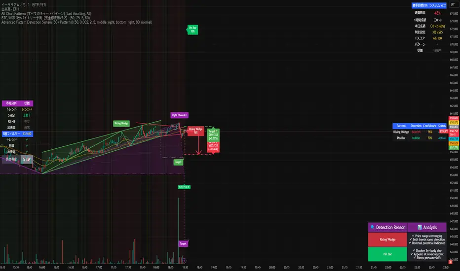
MaxAlgo - HTF Bias TableHTF Bias Tracker
Overview
The HTF Bias Tracker is a custom indicator designed to help traders monitor higher time frame (HTF) market biases while trading on lower time frames. It provides a clear visual table displaying the bias (bullish, bearish, mixed, or neutral) based on whether the current HTF candle has broken the high or low of the previous HTF candle. Additionally, it shows the current candle's condition (bullish or bearish based on close relative to open). This tool is particularly useful for multi-timeframe analysis, allowing traders to align lower time frame entries with higher time frame trends without switching charts.
The indicator does not generate buy/sell signals but offers contextual bias information to inform trading decisions. It is built for flexibility, supporting up to 5 customizable time frames (default: 1H, 4H, Daily, Weekly, Monthly) and can be used on any chart time frame.
How It Works
For each selected higher time frame (HTF):
Bias Calculation (H/L Break Column):
The indicator checks if the current HTF candle's high has exceeded the previous HTF candle's high (bullish break) or if the low has fallen below the previous HTF candle's low (bearish break).
Bullish: Current high > previous high (no low break).
Bearish: Current low < previous low (no high break).
Mixed: Both high and low breaks occur.
Neutral: No breaks yet. In this case, the text is colored based on the last completed break from the prior candle (green for bullish, red for bearish, orange for mixed) to maintain context.
Candle Condition (Candle Column):
Determines if the current HTF candle is bullish (close > open) or bearish (close <= open).
The results are displayed in a table with arrows (↑ for bullish, ↓ for bearish, ↔ for mixed) and color-coded text for quick readability.
The bias updates in real-time as the HTF candle develops, but final confirmation occurs at the HTF candle close.
This logic is rooted in price action principles: breaking a previous candle's extreme often indicates momentum. For example, historical data across various markets shows that when a candle takes the low of the previous candle, there's approximately a 70% probability it closes bearish (and vice versa for highs closing bullish). This can help gauge the likelihood of trend continuation, but results vary by asset, time frame, and market conditions—always backtest for your setup.
Features
Customizable Time Frames: Select up to 5 HTFs via inputs (e.g., "60" for 1H, "D" for Daily). Leave blank to disable.
Table Display: A compact table shows TF, H/L Break bias, and Candle condition. Includes headers for clarity.
Visual Enhancements: Color-coded text (green for bullish, red for bearish, orange for mixed, gray for neutral without prior bias). Arrows provide at-a-glance direction.
User Options:
Table Background Color: Adjust transparency and color for better visibility.
Table Position: Choose from 9 positions (e.g., Bottom Right default).
Border Width (Padding): Increase for more spacing around the table (min 0).
No Overlays: The indicator appears as a non-overlay pane, keeping your chart clean.
Supports all symbols and time frames, but best on lower TFs (e.g., 1m-15m) for monitoring HTFs.
How to Use It
Add to Chart: Search for "HTF Bias Tracker" in TradingView's indicator library and add it to your chart.
Configure Inputs: Set your desired HTFs, position, and colors.
Interpret the Table:
Look for alignment across multiple HTFs (e.g., multiple "Bullish ↑" biases suggest upward momentum).
Use the H/L Break as a directional filter: Enter long trades only when HTF bias is bullish or neutral with a prior bull break.
Combine with Candle Condition for confirmation: A bearish bias with a bearish candle might signal short opportunities.
Trading Example:
On a 1m chart, if the 1H bias shows "Bearish ↓" (low of previous 1H broken), there's ~70% chance the 1H closes lower. Wait for lower TF pullbacks to enter shorts, aligning with the HTF downtrend.
For scalping: If Daily is "Bullish ↑" but 4H is "Neutral ↓" (prior bear break), consider fading minor pullbacks but avoid counter-trend trades.
Risk Management: Always use stop-losses based on recent highs/lows and position size appropriately. This indicator aids bias assessment but should be combined with other tools like support/resistance or oscillators.
Strategy Ideas:
Trend Alignment: Trade in the direction of the majority HTF biases.
Breakout Confirmation: When a break occurs, monitor for volume or price action confirmation on your trading TF.
Reversion Plays: In ranging markets, a "Mixed ↔" bias might signal indecision—avoid trades until resolution.
Backtest the probability edge (e.g., via Pine Script strategies) to quantify performance in your markets.
Limitations and Disclaimer
The ~70% probability mentioned is a general observation from historical price action studies (e.g., across forex and indices); it is not a guarantee and should be verified with your own data. No backtesting results are provided here—users are encouraged to test independently.
The indicator relies on request.security() for HTF data, which may have minor delays in real-time.
This is not financial advice. Trading involves risk, and past performance does not predict future results. Use at your own discretion and consult a professional advisor if needed.

Ichimoku HorizonIchimoku Horizon – Multi-Timeframe Analysis
A multi-timeframe Ichimoku faithful to Hosoda, with authentic real-time calculations.
Ichimoku Horizon is an indicator based on the original method developed by Goichi Hosoda in the 1930s. It strictly respects the authentic formulas and prioritizes mathematical fidelity.
Key Features
Intelligent Multi-Timeframe
Native chart: Ichimoku from your trading timeframe
3 higher timeframes: Daily (1D), Weekly (1W), Monthly (1M) by default
Automatic projection: only higher timeframes relative to the chart are displayed
Precise offsets: displacement adapted to each timeframe
Guaranteed Authenticity
Hosoda’s original formulas fully respected
lookahead_off exclusively: lines calculated in real time with the current candle
Traditional displacement: 26 periods for cloud projection and Chikou shift
Why lookahead_off?
lookahead_off is the calculation mode that respects Hosoda’s logic:
Tenkan, Kijun, SSA and SSB all include the current candle and move in real time.
Chikou is the only exception: shifted 26 periods but calculated only with confirmed closes.
This way, what you see always matches the actual market as it is forming.
What is the no repaint approach?
A no repaint indicator displays values exactly as they exist in the present moment:
Lines update in real time during the formation of a candle.
Once the candle closes, they remain permanently fixed.
This ensures that the plots reflect the true construction of the market.
Main Parameters
Tenkan: 9 periods (short term)
Kijun: 26 periods (medium term)
SSB: 52 periods (long term)
Displacement: 26 periods (+26 for the cloud, −26 for the Chikou)
Timeframe Selection
TF1: Daily (structure aligned with trading activity)
TF2: Weekly (intermediate trend)
TF3: Monthly (macro vision)
Example Configurations
Scalping: Chart 1m → TF1: 5m, TF2: 15m, TF3: 1H
Intraday: Chart 5m → TF1: 15m, TF2: 1H, TF3: 4H
The indicator automatically hides inconsistent timeframes (lower than the chart).
Natural Line Display
Some lines will sometimes appear flat or straight: this is the normal behavior of Ichimoku, directly reflecting the highs and lows of their calculation windows.
Conclusion
Ichimoku Horizon is designed to remain true to Hosoda’s vision while offering the clarity of a modern multi-timeframe tool.
It delivers authentic, real-time calculations with no compromise.

RSI deyvidholnik
📊 Overview
RSI deyvidholnik is an advanced technical indicator that combines the power of traditional RSI (Relative Strength Index) with automatic divergence detection to identify potential market reversal points. This indicator was developed by kingthies and offers clear visual analysis of overbought/oversold conditions along with highly precise divergence signals.
🔧 Key Features
Customizable RSI
Data Source: Configurable (default: close)
Period: Adjustable (default: 14)
Moving Average: Multiple types available (SMA, EMA, SMMA, WMA, VWMA, MMS)
MA Period: Configurable (default: 14)
Divergence Detection
The indicator identifies four types of divergences:
🟢 Bullish Divergence
Occurs when price makes lower lows, but RSI makes higher lows
Indicates possible trend reversal from bearish to bullish
Signaled with green dots on RSI
🔴 Bearish Divergence
Occurs when price makes higher highs, but RSI makes lower highs
Indicates possible trend reversal from bullish to bearish
Signaled with red dots on RSI
🟢 Hidden Bullish Divergence (Optional)
Price makes higher lows while RSI makes lower lows
Confirms continuation of bullish trend
Useful in trending markets
🔴 Hidden Bearish Divergence (Optional)
Price makes lower highs while RSI makes higher highs
Confirms continuation of bearish trend
Useful in trending markets
⚙️ Pivot Settings
Optimized Default Configuration
Right Bars: 1 (quick confirmation)
Left Bars: 5 (noise filtering)
Maximum Bars Between Pivots: 60
Minimum Bars Between Pivots: 3
These settings have been adjusted to provide:
✅ Faster and more responsive signals
✅ Reduction of false signals
✅ Better identification of significant pivots
🎨 Visual Interface
RSI Levels
Line 70: Overbought zone (red)
Line 50: Neutral centerline
Line 30: Oversold zone (green)
Gradient fill: Visually intensifies extreme zones
Graphical Elements
RSI: Main line in white
Moving Average: Smoothed yellow line
Divergence Points: Colored markers on pivots
Background: Subtle fill for better readability
📈 How to Use
For Reversal Trading
Enable only: Bullish and Bearish (default)
Look for: Divergences in overbought/oversold zones
Confirm with: Other indicators or price analysis
For Trend Trading
Enable: Hidden Bull and Hidden Bear
Use in: Markets with clear established trends
Combine with: Market structure analysis
Alert Configuration
The indicator includes automatic alerts for:
⚠️ Bullish Divergence
⚠️ Bearish Divergence
⚠️ Hidden Bullish Divergence
⚠️ Hidden Bearish Divergence
💡 Main Advantages
✅ Automatic Detection: Identifies divergences without manual interpretation
✅ Optimized Configuration: Default values tested for maximum efficiency
✅ Clean Interface: Clear and professional visual
✅ Integrated Alerts: Automatic signal notifications
✅ Flexibility: Multiple customization options
✅ Performance: Optimized code for efficient execution
🎯 Recommended Timeframes
Scalping: 1m, 5m (with more sensitive settings)
Intraday: 15m, 30m, 1h (default configuration)
Swing: 4h, 1D (for medium-term signals)
⚠️ Important Considerations
Not infallible: Always use in conjunction with other analysis methods
Sideways markets: More effective in markets with directional movement
Confirmation: Always wait for signal confirmation before trading
Risk management: Always implement adequate stop-loss and take-profit

RSI Dynamic Bands█ OVERVIEW
The "RSI Dynamic Bands" indicator is a variant of the Relative Strength Index (RSI) oscillator that brings its signals directly onto the price chart. It displays dynamic bands around the price, adjusted based on RSI levels, enabling easy identification of potential overbought or oversold conditions. The indicator also integrates a multi-timeframe RSI table, facilitating the analysis of trend strength across different timeframes.
█ CONCEPTS
The "RSI Dynamic Bands" indicator is designed to simplify the interpretation of price levels in the context of support and resistance zones, which can be correlated with other technical indicators and RSI values. Since the price itself does not display RSI values, a table showing RSI for four selected timeframes has been added, allowing traders to quickly assess trend strength across different time intervals. The most effective approach is to combine the indicator with other technical analysis tools, such as Fibonacci levels or pivot points, to confirm signals when the price approaches the bands and RSI values indicate a potential reversal.
Band Calculation
The bands are calculated based on the current closing price and RSI values, incorporating dynamic scaling to better adapt to market conditions. The formulas for the bands are as follows:
• Upper Band: close + (rsiUpper - rsi) * scaleFactor, where rsiUpper is the upper RSI level (default: 70), and scaleFactor accounts for market volatility.
• Lower Band: close + (rsiLower - rsi) * scaleFactor, where rsiLower is the lower RSI level (default: 30).
• Midline: The arithmetic average of the upper and lower bands: (upperBand + lowerBand) / 2.
Why Scaling? Without scaling, the bands would be chaotic and jagged, making them difficult to interpret. Scaling smooths the bands, making them wider during periods of high volatility and narrower during consolidation, better reflecting potential support and resistance levels.
Indicator Features
• Dynamic Price Bands: The bands adapt to market conditions, facilitating the identification of key price levels.
• Multi-Timeframe RSI Table: Displays RSI values for four selected timeframes (default: 15m, 1h, 4h, Daily), enabling comparison of trend strength across different perspectives.
• Style Customization: Users can adjust band colors, line thickness, and toggle the visibility of bands, fills, and the table.
How to Set Up the Indicator
1 — Add the "RSI Dynamic Bands" indicator to your TradingView chart.
2 — Configure parameters in the settings, such as RSI length, upper/lower levels, and scaling multiplier, to match your trading style.
3 — Enable or disable the display of bands, fills, or the RSI table based on your needs.
4 — Adjust band and table colors in the input section and line thickness in the "Style" section to better align the indicator with your chart.
█ OTHER SECTIONS
FEATURES
• RSI Length: The period for calculating RSI (default: 14).
• RSI Levels: Thresholds for overbought (default: 70) and oversold (default: 30).
• Scaling Multiplier: Adjusts bands based on market volatility (default: 0.15).
• Table Timeframes: Select four timeframes for the RSI table (default: 15m, 1h, 4h, Daily).
• Style Options: Customize band colors, fills, table, and line thickness.
HOW TO USE
Add the indicator to your chart, configure the parameters, and observe price interactions with the bands to identify potential entry and exit points. The RSI table allows you to compare RSI values across different timeframes, aiding in trading decisions. The most effective approach is to combine the indicator with other technical analysis tools, such as Fibonacci levels or pivot points, to confirm signals when the price approaches the bands and RSI values indicate a potential reversal.
Trading Strategies:
• Scalping: Use lower timeframes (e.g., 5m, 15m) in the RSI table to quickly identify short-term lows and highs. Wait for the price to approach the lower band in the RSI oversold zone, with RSI on lower timeframes starting to rise, and other tools, such as Fibonacci levels (e.g., 38.2%) or pivot points, confirming support.
• Medium-Term Trading: Focus on 1h and 4h timeframes. Look for confirmation of a low on a lower timeframe (e.g., 1h), where RSI indicates oversold conditions or starts rising, then check if RSI on a higher timeframe (e.g., 4h) confirms the trend. Confirmation from other tools, such as a Fibonacci level (e.g., 50%) or pivot point near the bands, strengthens the signal.
• Long-Term Trading: Use Daily and higher timeframes (e.g., Weekly). Wait for all relevant timeframes to confirm a low (e.g., RSI near oversold and price at the lower band), with lower timeframes (e.g., 4h) showing rising RSI. Other tools, such as Fibonacci levels (e.g., 61.8%) or pivot points near the bands, can further confirm a trend reversal signal.

KSL-Fullsystem🔥 KSL Indicator คืออะไร? ใช้งานยังไงให้แม่นยำสุดๆ?
KSL คืออินดิเคเตอร์อัจฉริยะที่ช่วยบอก “จุดเปลี่ยนสำคัญของราคา”
ไม่ใช่แค่ดูกราฟมั่ว ๆ แล้วเดาสุ่ม!
📌 จุดเด่นของ KSL คือ “กรอบสีเขียว/แดง”
เมื่อราคามีแรงซื้อหรือแรงขายรุนแรง KSL จะสร้าง กรอบสีเขียว (Buy) หรือ กรอบสีแดง (Sell) ขึ้นมาทันที เพื่อแสดงให้เห็นว่า "ตรงนี้แหละ! คือจุดที่ตลาดมีแรงจริง!"
แต่จำไว้...
อย่ารีบเข้าออเดอร์ทันที!
✅ วิธีใช้งานที่แม่นยำ (เข้าใจง่ายมาก!)
🔹 ขั้นที่ 1: รอให้เกิดสัญญาณ (กรอบขึ้น)
🔹 ขั้นที่ 2: รอราคาย่อ / ดีดกลับมา “แตะกรอบ”
🔹 ขั้นที่ 3: ถ้ามีแรงกลับตัว → เข้าออเดอร์!
📍 กรอบสีเขียว/แดง = โซนต้นทางของแรง
คือโซนที่มีโอกาสเกิดแรงซื้อหรือขายซ้ำอีกครั้ง
ทำให้การเข้าเทรดของคุณ “แม่นยำขึ้น ปลอดภัยขึ้น”
🕒 ใช้ได้ทุก Timeframe ตั้งแต่ M1 ถึง H4
TF ใช้ยังไง จุดเข้า SL TP
M1-M5 เทรดเร็ว จบไว รอแตะกรอบแล้วเข้า นอกกรอบนิดเดียว ตามเป้าส่วนตัว
M15-M30 เห็นแนวโน้มชัด รอรีเทสต์แล้วแท่งย้ำทิศ SL นอกกรอบ TP ตามจังหวะ
H1-H4 เทรนด์แรง เทรนด์ยาว รอกลับตัวจากกรอบ SL นอกกรอบ เหมาะกับสาย Swing
💡 สรุปเข้าใจง่าย ๆ
❌ ห้ามเทรดทันทีหลังเห็นสัญญาณ!
✅ ให้รอราคากลับมาแตะกรอบก่อน
เพราะ:
🔹 กรอบ = จุดเริ่มต้นของแรง (เหมือน Supply/Demand Zone)
🔹 การเข้าเมื่อราคาย้อนกลับมา จะลดความเสี่ยง “ไล่ราคา”
🔹 ช่วยให้ได้จุดเข้าแม่น + SL สั้น + RR ดีขึ้น
📲 อยากลองใช้ KSL Indicator?
ทักมาเลยครับ! ทีมงานพร้อมสอนการใช้งานแบบ Step-by-step
ให้คุณเทรดได้อย่างมั่นใจ ไม่ต้องเดาทิศตลาดอีกต่อไป!
📍 ติดต่อผ่านไลน์: @kslacademy
หรือคลิกเลย: 👉 lin.ee/s5tk5BF
🔥 What is the KSL Indicator? How to Use It Accurately Like a Pro?
KSL is a smart trading indicator that helps identify critical price turning points —
Forget guessing or relying on random chart patterns!
📌 Key Feature: Green/Red Zones
Whenever there’s strong buying or selling pressure, KSL immediately highlights a
Green Box (Buy Signal) or Red Box (Sell Signal) to show you:
“This is where the real momentum started!”
But here’s the catch…
Never enter a trade immediately after the signal!
✅ How to Use KSL for Maximum Accuracy
🔹 Step 1: Wait for a signal box to appear
🔹 Step 2: Wait for price to pull back and retest the box
🔹 Step 3: If there's a sign of reversal → Enter your trade!
📍 The Green/Red Box = Origin Zone of Momentum
It’s where buy/sell pressure may happen again,
giving you a high-probability entry point.
🕒 Works on All Timeframes (M1 to H4)
Timeframe Usage Strategy
M1–M5 Fast scalping: Wait for retest and enter. Keep SL just outside the box.
M15–M30 Clearer trend: Wait for retest + confirmation candle. SL outside box, TP based on trend.
H1–H4 Strong swing trades: Wait for reversal signal at the box. SL outside box. Best for longer moves.
💡 Quick Summary
❌ Don’t jump in right after the signal!
✅ Wait for price to retest the box first.
Why?
🔹 The box = origin of real momentum (like a supply/demand zone)
🔹 Retesting gives a safer entry with better risk/reward
🔹 Helps avoid chasing price and getting trapped
📲 Ready to try KSL Indicator?
Message us now! Our team will guide you step-by-step
so you can trade with confidence — no more second-guessing the market!
📍 LINE: @kslacademy
👉 Or click: lin.ee/s5tk5BF

Adaptive Weighted Regression Channel (AWRC)Short Description:
The Adaptive Weighted Regression Channel (AWRC) is an advanced technical analysis tool that plots a dynamic regression channel based on the recent price action. The centerline is a linear regression (trendline) fitted to the selected price source over a rolling window. The channel boundaries are placed above and below the regression line by a user-selected multiple of the weighted standard deviation.
What makes AWRC unique is its ability to optionally weight each bar’s importance in the regression using Volume, ATR (Average True Range), or Recency Decay, offering a channel that can adapt to market volatility, participation, or trend acceleration.
Parameter Explanations:
length: Number of bars for the regression window (how many recent candles are included). Higher values = smoother, less sensitive channel.
StdDev Multiplier (mult): Controls the channel width. 2.0 is classic; higher = wider channels, lower = tighter.
Enable Weighting?: Turn ON to activate weighting of each bar. If OFF, all bars are equally weighted (classic regression channel).
Weight Type: Select what to use for weights (only active if Enable Weighting is ON):
"Volume": Higher volume bars have more influence on the regression.
"ATR": Bars with higher volatility (as measured by ATR) have more influence.
"Decay": More recent bars are given more weight (controlled by Decay parameter).
Decay: If Weight Type is "Decay", this controls the rate of recency decay. (e.g. 0.98 = slow decay; 0.90 = fast decay; values close to 1 mean a longer memory.)
Source for the calculation (src): Selects which price is regressed. Default is hl2 (average of high and low); you can choose close, open, etc.
Recommended Parameters:
For general use: length = 34, mult = 2.0, Enable Weighting = OFF, src = hl2
For volume-aware channel: Enable Weighting = ON, Weight Type = "Volume"
For volatility sensitivity: Enable Weighting = ON, Weight Type = "ATR"
For extra focus on recent price: Enable Weighting = ON, Weight Type = "Decay", Decay = 0.95 or 0.98
For swing trading: length = 21–55, mult = 1.5–2.5
For intraday/scalping: length = 10–20, mult = 1.0–1.5
Usage Tips:
The regression line shows the "best fit" trend for the selected window.
The channel captures the typical range; price breaking outside the channel can signal strength, exhaustion, or breakout.
Volume and ATR weighting help the channel adapt to market participation or volatility spikes.
Decay weighting locks onto the most recent trend direction quickly.
Adjust parameters to fit your timeframe and market volatility.
Use AWRC to spot trending moves, reversals, or overextensions.
Try different weighting and channel settings to match your trading style!
Mohammad - Auto TrendLinesMohammad - Auto TrendLines
Overview
An advanced automatic trendline detection system that identifies and draws both major and minor trendlines based on pivot highs and lows. This indicator uses sophisticated algorithms to detect market structure and automatically plot relevant trendlines, helping traders identify key support and resistance levels without manual chart analysis.
Key Features
Automatic Detection: Identifies pivot points and connects them to form trendlines without manual intervention
Multi-Level Analysis: Distinguishes between Major and Minor trendlines, both External and Internal
Smart Validation: Only draws trendlines that haven't been violated by price action
Comprehensive Alerts: 16 different alert conditions for breaks and reactions to trendlines
Fully Customizable: Complete control over colors, styles, widths, and display preferences for each trendline type
How It Works
The indicator uses a ZigZag algorithm with configurable pivot periods to identify significant highs and lows. It then connects these points to form trendlines, validating them against historical price action to ensure they remain relevant. The system categorizes trendlines into Major/Minor and External/Internal based on their significance in the market structure.
Use Cases
This indicator is particularly useful for:
Identifying trend continuations and potential reversals
Finding optimal entry and exit points based on trendline breaks
Setting stop-loss levels using trendline support/resistance
Confirming trade setups with multiple timeframe analysis
Automating trendline detection for systematic trading strategies
Settings/Parameters
Pivot Period: Controls the sensitivity of pivot detection (default: 5)
Display Options: Toggle visibility for each of the 8 trendline types
Style Customization: Adjust color, line style, width, and extension for each trendline
Alert Configuration: Enable/disable alerts for breaks and reactions to each trendline type
Delete Previous: Option to remove old trendlines when new ones are formed
How to Use
Add the indicator to your chart and adjust the Pivot Period based on your trading timeframe
Configure which trendline types you want to display (Major/Minor, External/Internal, Up/Down)
Set up alerts for the specific trendline interactions you want to monitor
Look for price reactions at trendlines for potential trade entries
Use trendline breaks as confirmation for trend changes
Signals
Break Alerts: Triggered when price closes beyond a trendline
React Alerts: Triggered when price touches but respects a trendline
Major External: Most significant trendlines based on major pivot points
Major Internal: Secondary major trendlines within the trend structure
Minor External: Short-term trendlines for intraday movements
Minor Internal: Smallest scale trendlines for precise entries
Trendline Types Explained
Up Trendlines: Connect ascending lows, act as support
Down Trendlines: Connect descending highs, act as resistance
External: Connect the outermost pivots
Internal: Connect pivots within the major structure
Best Timeframes
Works effectively on all timeframes:
Scalping: 1m, 5m, 15m charts
Day Trading: 15m, 1H, 4H charts
Swing Trading: 4H, Daily, Weekly charts
Position Trading: Daily, Weekly, Monthly charts
Important Notes
The indicator repaints trendlines as new pivots form - this is by design to maintain accuracy
Historical trendlines that have been broken are automatically extended to show past levels
Use multiple timeframe analysis for best results
Combine with other indicators for trade confirmation
Always use proper risk management
Alert Integration
This indicator uses the TradingFinder Alert Library for enhanced alert functionality, providing detailed notifications for all trendline interactions.
Version History
v6: Current version with full alert integration and enhanced trendline validation
Disclaimer: This indicator is for educational and informational purposes only. Past performance does not guarantee future results. Always conduct your own analysis and use proper risk management when trading.
Note: This is an overlay indicator that draws directly on your price chart. Ensure you have sufficient chart history loaded for optimal performance.
Superdupermegadeduper signals by BrenFX🚀 Superdupermegadeduper Signals by BrenFX
Overview
The Superdupermegadeduper Signals indicator is a comprehensive trading system that combines multiple advanced technical analysis concepts to identify high-probability trading opportunities. This indicator integrates supply/demand zone analysis, dynamic trendline detection, and multi-confirmation signal generation to provide traders with precise entry, stop-loss, and take-profit levels.
🎯 Key Features
Supply & Demand Zone Detection
Intelligent Zone Identification: Automatically detects high-probability supply and demand zones based on price action and touch frequency
Customizable Zone Strength: Set minimum touches required for zone validation (2-10 touches)
Visual Zone Display: Clear visual representation with customizable colors and transparency
Zone Extension: Projects zones forward for future reference
Dynamic Trendline Analysis
Multi-Touch Trendline Detection: Identifies significant support and resistance trendlines with configurable minimum touch requirements
Automatic Trendline Drawing: Draws and extends trendlines automatically with custom colors
Deviation Tolerance: Configurable deviation percentage for trendline validation
Breakout & Retest Signals: Detects trendline breakouts and subsequent pullback retests
Advanced Signal Generation
Dual Signal Types:
Zone Reversal Signals: Based on supply/demand zone interactions
Trendline Breakout Signals: Based on trendline breaks with pullback confirmation
Multi-Confirmation System:
Volume confirmation (optional)
RSI filter integration
Candlestick pattern confirmation
Pullback verification
Professional Trade Management
Multiple Stop Loss Methods:
ATR-based dynamic stops
Zone-based stops
Fixed point stops
Automatic Level Calculation: Entry, stop-loss, and take-profit levels calculated automatically
Real-Time Trade Table: Live display of current trade levels and parameters
Customizable Table Position: Place trade information anywhere on your chart
Alert System
Comprehensive Alerts: Get notified instantly when signals are generated
Detailed Alert Messages: Include entry price, stop-loss, and take-profit levels
Frequency Control: Once-per-bar alert frequency to avoid spam
📊 How It Works
Signal Logic
Zone Analysis: The indicator scans for areas where price has repeatedly found support or resistance
Trendline Detection: Identifies significant trend lines by connecting pivot points with multiple touches
Confirmation Process: Multiple filters ensure signal quality:
Price action confirmation (multiple bullish/bearish candles)
Volume above average (optional)
RSI oversold/overbought conditions (optional)
Entry Timing: Signals are generated when all confirmations align
Buy Signals Generated When:
Price reaches a demand zone with bullish reversal confirmation, OR
Price breaks above resistance trendline and retests successfully
Sell Signals Generated When:
Price reaches a supply zone with bearish reversal confirmation, OR
Price breaks below support trendline and retests successfully
⚙️ Configuration Options
Supply/Demand Settings
Zone Strength: Minimum touches required (2-10)
Lookback Period: Historical bars to analyze (10-100)
Zone Extension: Forward projection length (1-20 bars)
Trendline Settings
Lookback Period: Historical analysis range (20-200 bars)
Minimum Touches: Required pivot connections (2-5)
Deviation Tolerance: Allowable price variance (0.01-1.0%)
Signal Filters
Reversal Confirmation: Required confirmation candles (1-5)
Pullback Confirmation: Retest validation period (1-5)
Volume Filter: Above-average volume requirement
RSI Filter: Overbought/oversold confirmation
Trade Management
Stop Loss Methods: ATR, Zone-based, or Fixed points
ATR Multiplier: Risk adjustment (0.5-5.0x)
Take Profit: Fixed point target (1.0-50.0 points)
📈 Best Practices
Recommended Settings
For Scalping: Lower zone strength (2-3), shorter lookback periods
For Swing Trading: Higher zone strength (4-6), longer lookback periods
For Trend Following: Enable trendline signals, use ATR-based stops
Risk Management
Always use the provided stop-loss levels
Consider position sizing based on stop-loss distance
Monitor the trade table for real-time level updates
Use alerts to avoid missing opportunities
🎨 Visual Elements
Supply Zones: Red semi-transparent rectangles
Demand Zones: Green semi-transparent rectangles
Resistance Lines: Red trendlines
Support Lines: Green trendlines
Buy Signals: Green "BUY" labels below bars
Sell Signals: Red "SELL" labels above bars
Trade Table: Comprehensive trade information display
💡 Tips for Success
Combine with Market Structure: Use on clean trends and at key support/resistance levels
Multiple Timeframe Analysis: Confirm signals on higher timeframes
Volume Confirmation: Enable volume filter for higher quality signals
Risk Management: Never risk more than 1-2% per trade
Backtesting: Test settings on historical data before live trading
⚠️ Important Notes
This indicator works best in trending markets
Signals are more reliable when multiple confirmations align
Always consider fundamental analysis and market conditions
Past performance does not guarantee future results
Practice proper risk management at all times
🔧 Technical Specifications
Pine Script Version: 6
Overlay: Yes
Max Objects: 500 boxes, 500 lines
Performance: Optimized for real-time analysis
Compatibility: Works on all timeframes and instruments
Developed by BrenFX | Advanced Trading Signals for Professional Traders
Remember: Trading involves risk. This indicator is a tool to assist in analysis and should not be the sole basis for trading decisions. Always use proper risk management and consider your financial situation before trading.
🔁 A.X.I.S Fibonacci Engine V2 – Smart Projected Pathway🔁 A.X.I.S Fibonacci Engine V2 – Smart Projected Pathway indicator
The A.X.I.S Fibonacci Engine V2 is a next-generation Fibonacci projection tool designed for traders seeking advanced, adaptive levels that respond to true multi-timeframe market structure. Built from the ground up for active traders—scalpers, swing traders, and position players—it fuses traditional Fibonacci logic with dynamic price projection and smart anchor logic.
How It Works:
Multi-Timeframe Anchoring:
Anchors your Fibonacci levels to High Timeframe (HTF) pivots for powerful bias and “macro” market structure, while also utilizing Low Timeframe (LTF) swing detection for precise “micro” projection and pathway analysis.
Dynamic Pathway Projection:
Beyond static lines, this engine allows Fibonacci levels to be projected forward, following the price path between significant swings—giving you projected targets and active “pathways” instead of just fixed retracement bands.
Trend-Adaptive Logic:
Determines bullish/bearish bias based on where HTF price closes relative to a moving average (HTF EMA-20), meaning the plotted fibs automatically adjust to uptrends or downtrends. No need to guess direction.
Auto-Cleanup & Smart Management:
Old lines and labels are deleted automatically to keep your chart clean, and levels are recalculated with every new significant swing (“leg”)—no manual intervention needed.
Key Features:
Multi-Timeframe Input:
Choose both HTF (for “anchor” pivots) and LTF (for “projection” pivots) independently.
Fine-tune swing sensitivity for both anchors and pathway pivots.
Classic + Projected Mode:
Choose between standard horizontal Fibs or enable Dynamic Pathway Mode to project levels diagonally into future bars, creating “fib pathways.”
Color Customization:
Individualize bullish/bearish fib colors, line style (solid, dashed, dotted), thickness, label position, and transparency.
Special “golden zone” highlighting for the most critical levels (0.618/0.786).
Visual Anchors:
Optionally plot markers for HTF swing pivots for extra clarity.
Chart Cleanliness:
Script manages and deletes its own objects—no more chart clutter!
Real-Time Auto-Update:
All levels and pathways update in real time as market structure changes.
User-Friendly Labels:
Toggle on/off fib level labels, with position and background adjustments.
Practical Trading Applications:
Swing/Position Trading:
Use HTF pivots for macro context, then project LTF fibs into the future for potential reversal/extension targets.
Scalping:
Deploy on lower timeframes with micro pivots for intraday levels and short-term projected moves.
Dynamic Take-Profit & Entry Zones:
Identify evolving TP and re-entry zones as price carves out new swings, even in choppy or trending conditions.
Trend Confirmation:
Let the engine determine trend direction, so your fibs are always aligned with prevailing momentum.
How to Use:
Add to Chart:
Apply the indicator to any chart or timeframe.
Set Your Anchors:
Pick the HTF (anchor) and LTF (projection) timeframes.
Adjust swing sensitivity (lookback) as needed.
Enable/Disable Dynamic Pathway:
For regular fibs, leave off.
For projected “pathways,” turn it ON—lines will project forward along the likely path of the next move.
Adjust Colors, Labels, and Styles:
Fine-tune everything for clarity and your personal style.
Watch for Changes:
As new pivots form, the script will update levels in real time, keeping your roadmap fresh.
(Optional) Show Macro Swings:
Toggle on/off to plot markers for the most recent HTF pivots.
Who Is It For?
Day traders, scalpers, and swing traders wanting true projected price targets—not just static fibs.
Traders tired of redrawing fibs after every new swing.
Anyone who wants a clean, dynamic, and truly adaptive fib tool that blends macro and micro market structure into one engine.
What Makes It Different?
True multi-timeframe awareness:
Adapts to both macro (HTF) and micro (LTF) structure.
Automatic trend recognition:
Fibs align with price action—no manual flipping.
Projected, not just static:
See where fib levels could land, not just where they were.
Cleanest chart management:
Deletes its own lines and labels on every update—no mess, ever.
Note:
This tool is for educational and informational purposes only. Not financial advice. Always use proper risk management!
Any issues or feature requests? Drop a comment below or reach out!
Happy trading and welcome to the A.X.I.S revolution.
— I5X-Albatross
