SN30 IndicatorIndicator «SN30»
Class : oscillator
Trading type : scalping
Time frame : 5 min
Purpose : reversal trading
Level of aggressiveness : standard
Indicator « SN30 » is based on the linier regression and normal distribution. Regression is one of the most popular and effective methods of the time series analysis and data prediction. Indicator « SN30 » uses regression analysis as an alternative to the moving averages analysis. The main aim is data series smoothing to reduce the noise in data. It allows to see market as it is, without deformation.
Using unique author algorithm indicator « SN30 » searches for the optimal buy/sell zones. If they are sufficient indicator generates appropriate trading signals.
Structure of the indicator «SN30»
Indicator «SN30» consists of central channel line (green line based on linier regression) and price channels (2 blue and 2 red lines with colored zones between them). Colored zones are of two types: red (overbought zone) and blue (oversold zone). They are used to define deviations of the current prices from their fair values. When the price enters the red zone it should reverse soon (the prices will go down). The same is true for the blue zone (the prices will go up).
Also when the buy/sell signal is generated special signs are displayed on the chart (red and blue triangles)
Parameters of the «SN30» indicator
1. PeriodSN30 (indicator period, default value = 21) – is used to calculate fair value of the asset based on linier regression.
2. Width – defines the width of the stationary channel (indicated by bold lines). Default value = 20 pips.
3. Sigma – defines the width of the dynamic channel (indicated by usual lines). Default value = 2standard deviations. It allows fitting 95% of price values into channel. All the price values out of the channel are treated as abnormal.
Rules of trading
The indicator is designed to work on 5-minute time frames, but after additional adjustment of parameters it can be used on any other time periods.
The general principle of the “SN30” indicator is the same as that of any indicator of the oscillatory class: when the price is in the overbought zone it is interpreted as a signal of a future price reverse in the downward direction, and when the price is in the oversold zone it is a signal of a future price reverse in the upward direction.
The rules of trading are extremely simple: when the red triangle is appeared on the chart (sell signal) or a blue triangle (a buy signal), a corresponding transaction (sell or buy an asset) should be done. Stops can be placed above/below the red/blue zones.
"scalping" için komut dosyalarını ara

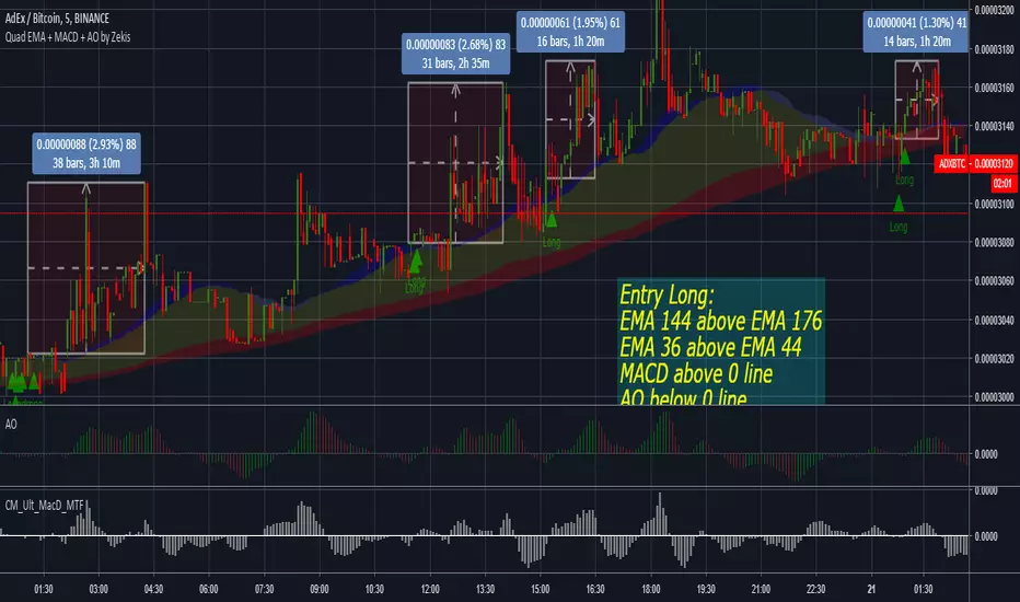
Quadruple EMA + MACD + Awesome Oscillator by ZekisThis strategy is based on quadruple EMAs, MACD and Awesome Oscillator, developed by Nenad Kerkez and simplified by me.
Scalping strategy (lower time frames)
Entry Position
Before we take a buy trade the two above criteria must be met. The 144 EMA must be above the 176 EMA and the 36 EMA must be above the 44 EMA. We then wait for AO to fall below the 0. The final „trigger‟ to the entry is when the MACD closes above the 0 line.
Sell trade is vice versa. 36 EMA must be below 44 EMA and 144 EMA must be below 176 EMA.
TAKE PROFIT and STOP LOSS
10-40 pips. Pivot Point targets.
STOP LOSS above/below last highest high
Enjoy!
@Zekis
Contrarian Scalping Entry Support v2.1This indicator is still making and testing now.
I don't recommend to use it without Pro / Prop TRADER.
// Copyright @ ALEX SHORT
// alpha tester : Norakichi Senpai (Santa Prop Norakichi Senpai)
// Special Thanks WBZ Trading Group
// This indicator support "Short term Fighting the tape Entry".
// Attension!!! I strongly reccomend to Verify effectiveness before "REAL TRADE".
// Note. Downtrend often continue compared to uptrend. So, you might have to change DFMA setting for it. Or you should change reasons/grounds for Scalping Long Entry in long DownTrend.
// Function1. Difference from moving average Arrow v 1.7 from SMA 200
// This indicator will plot chart Arrow above or below candle stick when DFMA marked over range.
// Function2. When price touch Quado_Bollinger band, background will change background and Circle Alert will plot above / below Candle stick.


Prometheus Scalping vs. Swinging by ZekisIt's been a while since i did not post a script, so here it is...
I found some simple indicators,put them together and saw some nice results.
There is an indicator for scalping, swinging and for exit.
With the right setup it can be very useful, so you can play with it to find what you need
It works in any timeframe in any market, just change values (default ones are good for 1H or more), all you need is volatility... (this is what you need in any market!)
Also you can enable or disable background and bar colors
Enjoy!
@Zekis

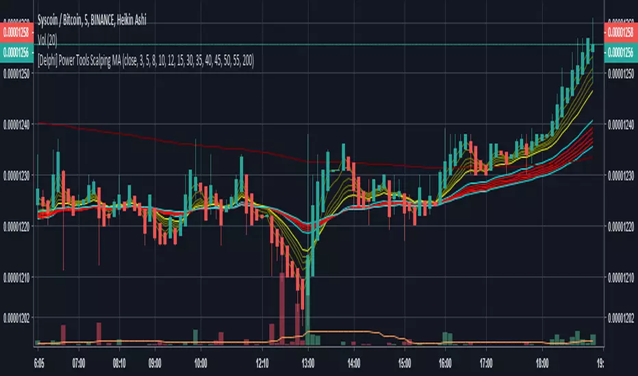
[Delphi] Power Tools Scalping MA Power Tools Scalping MA
Inner Version 1.0 01/01/2019
Developer: iDelphi
01/01/2019 Added Multi EMA Channel
BlockGain Candlestick for Scalping VER. 1.2This is a new tool for scalping with candleskick and EMAS .... show signals for buy and sell

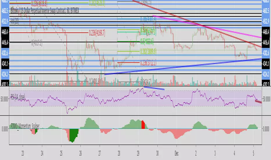
FOMO_Momentum_ScalperIndicator is easy to work with.
The histogram indicates the momentum.
Nothing fancy but signals are pretty accurate
Dark Green Bars on Histogram - Buying opportunity (Momentum of dump is decreasing)
Dark Red Bars on Histogram - Selling opportunity (Momentum of pump is decreasing)
Works best on 1m chart for those great scalping opportunities. Signals are based on increasing Buy/Sell momentum against the direction of the movement.
Haven't tested on any instrument except BTC.
Haven't tested for divergences but it should do the job.
P.S. It doesn't give too many signals as it waits for extreme conditions.
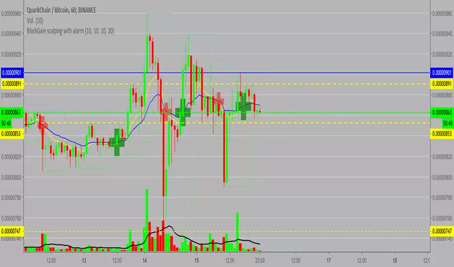
BlockGain scalping with alarmUse for sclaping 15min and 1H ... this indicator include alarm for long
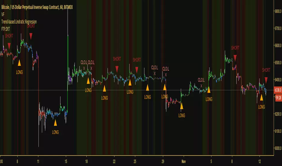
Trend-based Lindratic RegressionThis is an effective trend-following script that uses a finite volume element, linear regression, quadratic regression and multiple EMAs to define appropriate times to enter and exit the market. It can be applied to any asset that has volume data available for it.
As it follows the trend it's a very low-risk strategy, but it's not made to catch and ride reversals. It would rather close a long at the top and close a short at the bottom, although this means you can expect not to be stopped out on any trade you take.
Works on any timeframe, although I did create this with the intention of scalping, so shorter timeframes are recommended.
Combined with a volatility filter, this would be a very effective script, allowing you to stand away from the market during flat periods and trading with the trend during exciting periods.
Access to the script will be grated for 10$ of most low-fee cryptocurrencies, as well as BTC. If you're interested reach out to me through TradingView or, alternatively, contact @overttheraibow through Telegram.
If there's enough demand for it, I will also create a strategy version of this study which will be given for free to those who purchased the script. As always, maximum 250 places available.
Good luck!
Renko scalp (buy/sell) indicatorThis script is based on some variations of Rocket (from Until1Mil group) scalping strategies.
It uses Renko to determine buy/sell areas.
More details can be found on my steemit page (same user as here).

Renkonator 5000 [IND]Renko scalping indicator based off Vdub Renko SniperVX1 v1. Major addition is requiring confluence of MACD signal for opening position + alerts for entering long/short positions.
Important: use Traditional setting with Renko. Box Size and timeframe are the two most important settings to optimize for.
Suggestions:
Pair Box Size Timeframe
EURCAD 0.0001 240m
BTCUSD 1 240m
ETHUSD 0.1-1.0 240m

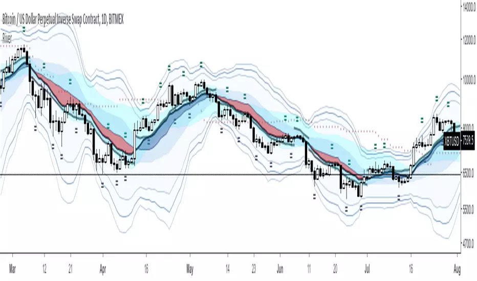
River Scalping (Fibonacci, Pivots, VWMA, BB, EMA)Pictured as a Scalping Indicator, it shines best on the H4 and specially on the D1.
A combination of too many Fibonacci progressions, Pivots, VWMA , EMA's, BB, Stochastic RSI, the Kijun (Doubled Ichimoku Cloud ), William's Fractals ('=') and too many Standard Deviations.
Simple Strategy :
Center Blue: Long
Center Red: Short
The river can unveil the market's momentum and its strength.
Don't only use the simple strategy, there is much more if you decide to fall down the rabbit hole.
Suggestions are, as always, more than welcomed,
Have fun out there and stay safe.
Please be advised, this indicator will only be free for a limited time.
VJ_Holy_Grail_ScalperA simple scalping indicator
Green triangle = Buy
Red triangle = Sell
Added buy/sell alerts for Autoview

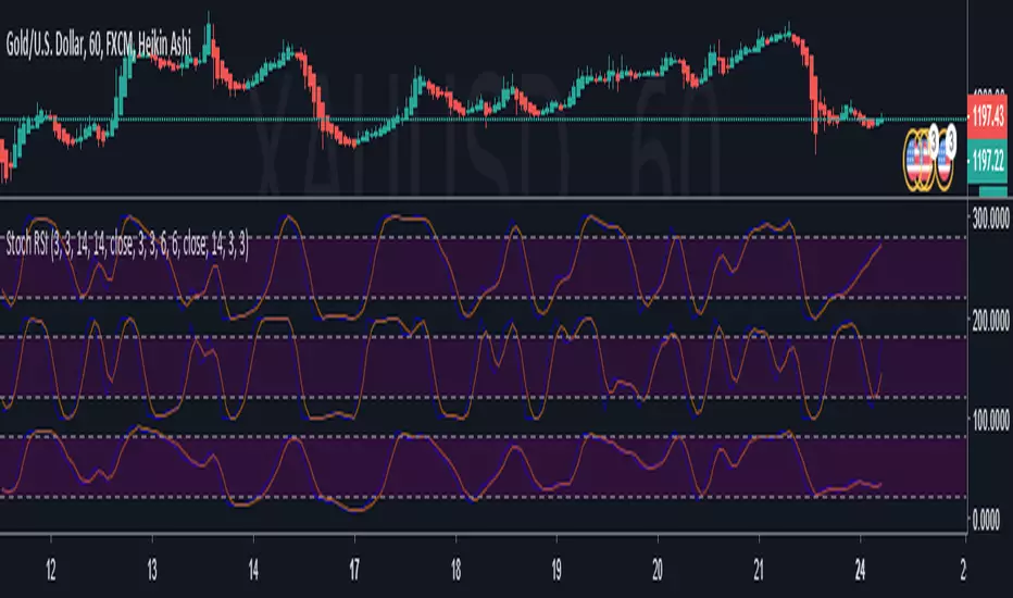
Triple Stochastic Strategy - Alejo Laos - NO ALERTThe stochastic triple looks for signs of entry in candles of 5 and 15 minutes to apply scalping strategy.
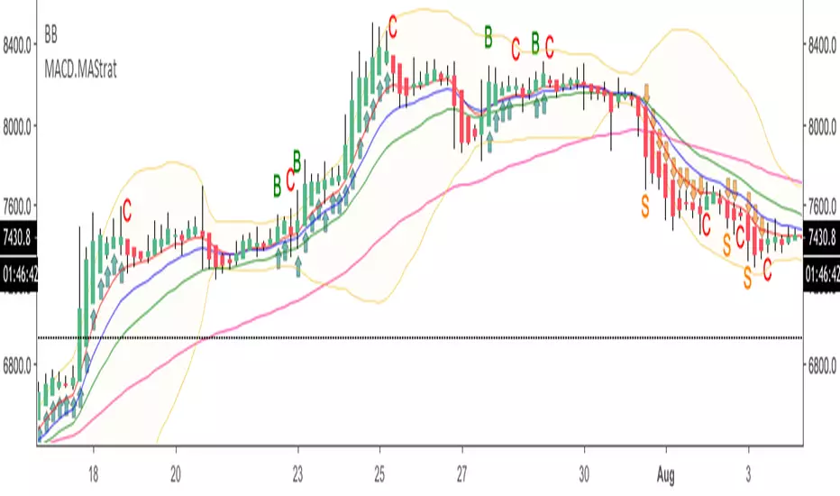
HA.MACD.MA.TradeSetupsHi probably trade setups indicator intended to be used with Heikin Ashi candles. It uses fibo EMAs and MACD to signal longs/shorts. Intended for scalping high cap coin with high volume on lower time frames.

Crypto Spiper Killer Pro [PlungerMen]Hello!
Crypto Spiper Killer Pro is a upgrade version of a Crypto Spiper Killer
Crypto Spiper Killer Pro can use for every coin
Crypto Spiper Killer Pro is available for all frames
This Script is perfectly functional and works well by me and the best way to use this script is to use it with “Bitmex Long Short" script, both compliment for each other. the "Bitmex Long Short" script is Free, you can find it by searching “Bimex”
If you want to be more accurate and more efficient, more comfortable when you do not want to see too many other indicators, you can register for our Professional edition.
- The Professional Edition supports Level 1 and Level 2 commands ( display at chart : LONG+, long-, SHORT,+,short- ), which are very effective in allocating funds and optimizing your profits
Besides that,You will be supported by personal preferences, profit maximization
- Register for a Professional version will be used 2 Script, Bitcoin -0.95% -3.33% -3.27% Scalping Pro and Bitmex Long Short Pro
- We will invite you to the signal channel Telgram with the announcement of the bottom and the peak of the BTC -0.95% -3.33% -3.27% 0.60% -0.13% ,the big variable variable has exists
**We hope you enjoy this script. Your support will help us develop more good quality scripts in the future to serve the community **
**Remember, Like this script and posivite feedback if you are satisfied**
if you have any questions, post a comment ... below here
*********** Guide:
+ option for all frames : Click setting and input high and low for time inteval
+ hide wave trend : Click setting -> click Style --> Up trend Fill or Down trend fill
******
New features: this time we add two lines that can help traders trader safer. When the red line cross above the green line means we are in the downtrend and when the green line cross above the red line, which means we are in a uptrend. This new features will help traders do a safer trade at small time frame.
We have the Script free for the user pass, search keyword " Crypto Spiper Killer Pro "
-->> 0.2 eth/1 month will be used 2 Script: Crypto Spiper Killer Pro and Bitmex Long Short Pro - and Super Bot telegram

DYNAMIC SUP/RES 1.0Dynamic Support / Resistance Indicator. Good for scalping ranging price action and detecting breakouts.
White area represents current range. Red lines are Stop Loss levels based on range and Risk to Reward ratio of choice.
Free to use for Cryptosurge discord members: discord.gg
Trade safe and DYOR.


