Stealth Trigger X🔰 Stealth Trigger X — Smart Divergence & Breakout Strategy with Trend Weakness Exit
Stealth Trigger X is a precision-engineered, non-repainting strategy designed for traders who rely on high-conviction breakouts and trend confirmation. Rather than relying on lagging or oversimplified signals, this strategy fuses divergence logic, volatility detection, volume filtering, and slope-based trend validation into one clean system — making it both responsive and reliable.
📌 Core Components (How It Works):
1. ZLEMA (Zero-Lag Exponential Moving Average):
Used as the primary trend baseline. Unlike a standard EMA, ZLEMA compensates for lag by using a double-smoothing technique that allows the strategy to detect trend direction changes sooner — especially useful in crypto and fast-moving markets.
2. Gradient Filter (Slope of ZLEMA):
Rather than waiting for price to cross a moving average, the strategy measures the slope of the ZLEMA itself. Positive slope = uptrend, negative slope = downtrend. This gives us early trend validation and exit signals based on weakening momentum.
3. Vortex Indicator (Directional Volatility):
A diff-based implementation of the Vortex Indicator is used to validate whether volatility is expanding in favor of the trend. This prevents false entries during indecision phases or low-momentum conditions.
4. White Line Bias Filter (Structural Trend):
The strategy calculates the midpoint of the highest high and lowest low over a user-defined period. This “White Line” serves as a structural trend bias, ensuring entries align with the broader context — not just momentary momentum.
5. Volume Spike Confirmation:
To avoid manipulation and choppy conditions, the strategy confirms breakouts only when the current bar’s volume exceeds the median volume of recent candles by a set multiplier. This filters out noise and ensures only high-conviction moves trigger entries.
6. Breakout with Divergence Timing:
A hybrid logic checks for price breaking previous range highs/lows (breakouts), combined with simulated divergence behavior based on RSI-like momentum. This helps align entry timing with areas where price is likely to accelerate.
⚙️ Trade Management Logic:
Entry Conditions:
Triggered when all conditions align: ZLEMA slope, Vortex confirmation, White Line bias, volume spike, and divergence-based breakout.
Take Profits:
TP1: 50% of position is closed using a limit order
TP2: Remaining 50% closed with another limit order
This split exit approach lets profits run while locking in gains early.
Exits on Trend Weakness:
If trend conditions weaken (slope flip or vortex flip), the position is exited before a full reversal occurs — helping protect capital during exhaustion phases.
Reentry Delay:
Enforces a 1-bar cooldown between exit and new entries to avoid “ping-pong” signals and maintain clean backtest results.
📊 Real-Time Dashboard (On-Chart):
Displays critical stats including:
Current position (Long, Short, or Flat)
Entry price
TP1 and TP2 hit status
Win rate (%)
Profit factor
Bars since entry
This makes live trading or visual backtesting easy to interpret and track.
✅ Key Facts:
Non-Repainting: All signals are calculated using confirmed bar data only. No future bars or security() functions are used.
Original Logic: This is not a generic mashup. Each component (ZLEMA slope, vortex diff, breakout divergence, volume spike filtering, White Line structure) is optimized to work in tandem.
Best Timeframes: 1H – 4H
Markets: Crypto, Forex, Indices — any market with trending behavior and measurable volume
⚠️ Disclaimer:
This strategy is for educational purposes only. It is not financial advice or a recommendation to trade. Past performance does not guarantee future results. Always trade with proper risk management and backtest strategies before live deployment.
🧠 Summary:
Stealth Trigger X is built for traders who want:
Precision entries
Early trend exits
Reliable backtest integrity
Clean logic with no repainting
It is especially effective in breakout environments where volume and momentum align — and excels at avoiding weak or manipulated trends.
"profit" için komut dosyalarını ara

Heiken Ashi Supertrend ADX - StrategyHeiken Ashi Supertrend ADX Strategy
Overview
This strategy combines the power of Heiken Ashi candles, Supertrend indicator, and ADX filter to identify strong trend movements across multiple timeframes. Designed primarily for the cryptocurrency market but adaptable to any tradable asset, this system focuses on capturing momentum in established trends while employing a sophisticated triple-layer stop loss mechanism to protect capital and secure profits.
Strategy Mechanics
Entry Signals
The strategy uses a unique blend of technical signals to identify high-probability trade entries:
Heiken Ashi Candles: Looks specifically for Heiken Ashi candles with minimal or no wicks, which signal strong momentum and trend continuation. These "full-bodied" candles represent periods where price moved decisively in one direction with minimal retracement.
Supertrend Filter : Confirms the underlying trend direction using the Supertrend indicator (default factor: 3.0, ATR period: 10). Entries are aligned with the prevailing Supertrend direction.
ADX Filter (Optional) : Can be enabled to focus only on stronger trending conditions, filtering out choppy or ranging markets. When enabled, trades only trigger when ADX is above the specified threshold (default: 25).
Exit Signals
Positions are closed when either:
An opposing signal appears (Heiken Ashi candle with no wick in the opposite direction)
Any of the three stop loss mechanisms are triggered
Triple-Layer Stop Loss System
The strategy employs a sophisticated three-tier stop loss approach:
ATR Trailing Stop: Adapts to market volatility and locks in profits as the trend extends. This stop moves in the direction of the trade, capturing profit without exiting too early during normal price fluctuations.
Swing Point Stop : Uses natural market structure (recent highs/lows over a lookback period) to place stops at logical support/resistance levels, honoring the market's own rhythm.
Insurance Stop: A percentage-based safety net that protects against sudden adverse moves immediately after entry. This is particularly valuable when the swing point stop might be positioned too far from entry, providing immediate capital protection.
Optimization Features
Customizable Filters: All components (Supertrend, ADX) can be enabled/disabled to adapt to different market conditions
Adjustable Parameters: Fine-tune ATR periods, Supertrend factors, and ADX thresholds
Flexible Stop Loss Settings: Each of the three stop loss mechanisms can be individually enabled/disabled with customizable parameters
Best Practices for Implementation
Recommended Timeframes: Works best on 4-hour charts and above, where trends develop more reliably
Market Conditions: Performs well across various market conditions due to the ADX filter's ability to identify meaningful trends
Position Sizing: The strategy uses a percentage of equity approach (default: 3%) for position sizing
Performance Characteristics
When properly optimized, this strategy has demonstrated profit factors exceeding 3 in backtesting. The approach typically produces generous winners while limiting losses through its multi-layered stop loss system. The ATR trailing stop is particularly effective at capturing extended trends, while the insurance stop provides immediate protection against adverse moves.
The visual components on the chart make it easy to follow the strategy's logic, with position status, entry prices, and current stop levels clearly displayed.
This strategy represents a complete trading system with clearly defined entry and exit rules, adaptive stop loss mechanisms, and built-in risk management through position sizing.

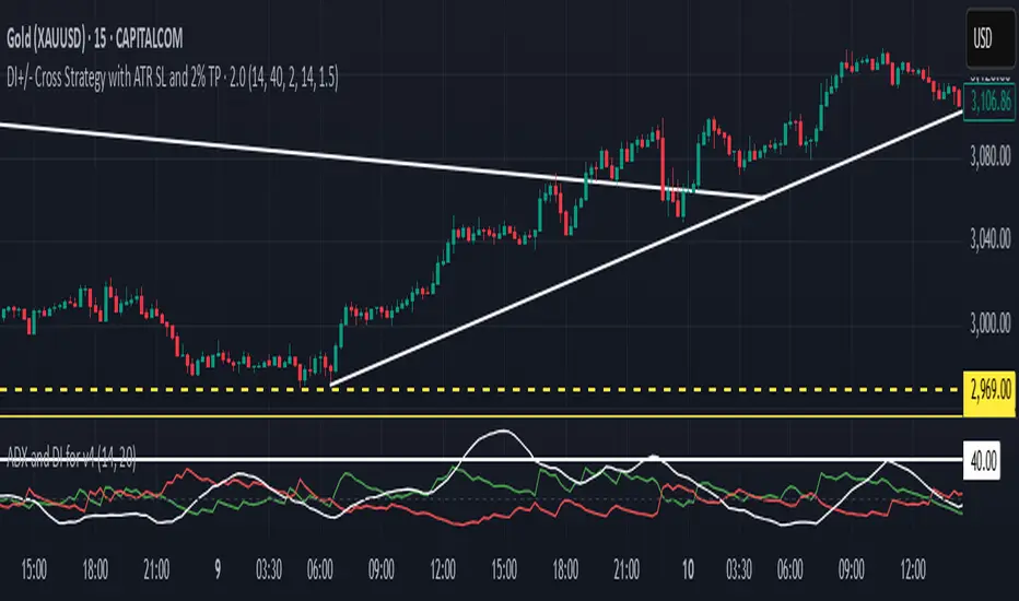
DI+/- Cross Strategy with ATR SL and 2% TPDI+/- Cross Strategy with ATR Stop Loss and 2% Take Profit
📝 Script Description for Publishing:
This strategy is based on the directional movement of the market using the Average Directional Index (ADX) components — DI+ and DI- — to generate entry signals, with clearly defined risk and reward targets using ATR-based Stop Loss and Fixed Percentage Take Profit.
🔍 How it works:
Buy Signal: When DI+ crosses above 40, signaling strong bullish momentum.
Sell Signal: When DI- crosses above 40, indicating strong bearish momentum.
Stop Loss: Dynamically calculated using ATR × 1.5, to account for market volatility.
Take Profit: Fixed at 2% above/below the entry price, for consistent reward targeting.
🧠 Why it’s useful:
Combines momentum breakout logic with volatility-based risk management.
Works well on trending assets, especially when combined with higher timeframe filters.
Clean BUY and SELL visual labels make it easy to interpret and backtest.
✅ Tips for Use:
Use on assets with clear trends (e.g., major forex pairs, trending stocks, crypto).
Best on 30m – 4H timeframes, but can be customized.
Consider combining with other filters (e.g., EMA trend direction or Bollinger Bands) for even better accuracy.
Dskyz Adaptive Futures Edge (DAFE)imgur.com/a/igj9lFj
Dskyz Adaptive Futures Edge (DAFE) is a futures trading strategy designed to adapt dynamically to market volatility and price action using a blend of technical indicators. The strategy combines adaptive moving averages, optional RSI filtering, candlestick pattern recognition, and multi-timeframe trend analysis to generate long and short trade signals. It incorporates robust risk management techniques including ATR-based stop-losses and trailing stops, ensuring trades are sized and managed within sustainable risk limits.
Key Components and Logic
-Adaptive Moving Averages
Dynamic Calculation: Fast and slow Simple Moving Averages (SMAs) adapt to changing volatility, making them sensitive to high-momentum shifts and smoothing during quieter price action.
Signal Generation: Entry signals are triggered when the fast SMA crosses the slow SMA in conjunction with price direction confirmation (e.g., price above both for long positions).
-RSI Filtering (Optional)
Momentum Confirmation: The RSI filter provides momentum confirmation to avoid overextended entries. It can be toggled on or off for both long and short conditions.
User Control: Adjustable parameters such as lookback period, oversold/overbought thresholds, and enable/disable switches give full control over its influence.
-Candlestick Pattern Recognition
Engulfing Logic: Recognizes strong bullish or bearish engulfing patterns with configurable strength criteria like range and volume. Patterns are filtered by trend direction and strength for confirmation.
Signal Conflict Handling: When both bullish and bearish engulfing patterns occur within the lookback window, the strategy avoids entry to reduce whipsaws in indecisive markets.
-Multi-Timeframe Trend Filter
Higher Timeframe Filtering: Incorporates 15-minute trend direction as a macro-level filter to align intrabar trades with larger trend momentum.
Smoothed Entry Logic: Prevents entering trades that go against the broader market structure, reducing false signals in choppy or low-conviction moves.
-Trade Execution and Risk Management
imgur.com
Entry Logic
Priority System: Users can define whether moving average signals or candlestick patterns should take priority when both are present.
Volume & Volatility Checks: Ensures sufficient market participation and action before entering a position, improving the odds of reliable follow-through.
Stop-Loss and Trailing Exit
ATR-Based Initial Stops: Dynamically adjusts stop-loss distance based on market volatility using a multiple of ATR (Average True Range), keeping risk proportional to price swings.
Trailing Stop: Protects open profits and enables winners to run by following price action at a set distance (also ATR-based).
-Cooldown Period & Minimum Bar Hold (Trade Discipline Logic)
Cooldown Bars: After an exit, the strategy imposes a mandatory pause before opening a new position.
Why: This avoids rapid-fire re-entries triggered by minor fluctuations that could lead to overtrading and degradation of profitability.
Minimum Bar Hold: A trade must be held for a minimum number of bars before it can be exited.
Why: This prevents the strategy from immediately exiting trades due to fleeting volatility spikes, which previously caused premature exits that often reversed back in favor of the original signal. This ensures trades have adequate time to develop, filtering out noise from true reversals.
-Visual Elements and Transparency Tools
Chart Overlays: Moving averages, RSI values, and trade entry/exit points are shown directly on the chart for complete visibility.
Dashboard UI: Displays critical live metrics—current position, PnL, time held, ATR values, etc.
Debug Logs: Optional toggles allow verbose condition tracking for deep inspection into why a trade occurred (or didn't), useful for both live optimization and debugging.
-Input Parameter Reference Guide
Input Name Function & Suggested Use
Use RSI Filter - Enables or disables RSI-based entry confirmation. Disable if price action alone is desired for entry decisions.
RSI Length - RSI lookback period. Lower values (e.g., 7–14) are more responsive; higher values reduce false signals.
Overbought / Oversold Levels - Used to detect exhaustion zones. E.g., avoid long entries above 70 or short entries below 30.
Use Candlestick Patterns - Enable detection of bullish/bearish engulfing patterns as trade signals. Disable to rely only on trend/MA.
Pattern Strength Thresholds (Range, Volume) - Filters out weak engulfing signals. Higher values require stronger patterns to trigger.
Use 15min Trend Filter - Adds multi-timeframe trend confirmation. Recommended for filtering entries against larger trend direction.
Fast MA - Base Length for fast adaptive moving average. Suggested: 10–25.
Slow MA - Base length for slow adaptive moving average. Suggested: 30–60.
Volatility Sensitivity Multiplier - Multiplies volatility adjustments for adaptive MA length. Higher = more reactive to volatility.
Entry Volume Filter - Filters out trades during low volume. Recommended to prevent entries in illiquid conditions.
ATR Length - Lookback period for ATR calculation. Suggested: 14.
Trailing Stop ATR Offset - Defines how far the stop-loss is from entry. 1.5–2.5 is typical for medium-volatility environments.
Trailing Stop ATR Multiplier - Determines trailing stop distance. 1.5 is tight; 3+ gives more room for trending trades.
Cooldown Bars After Exit - Prevents immediate re-entries. Suggested: 3–10 bars depending on timeframe.
Minimum Bars to Hold Trade - Ensures trades are held long enough to avoid knee-jerk exits. Suggested: 5–10 for intraday strategies.
Trading Hours (Start / End) - Sets the window of allowed trading. Prevents entries outside key session times (e.g., avoid pre-market).
Enable Logging / Debugging - Shows internal trade decision data for tuning and understanding the logic.
Compliance with TradingView Regulations
Realistic Backtesting: The strategy uses proper initial capital, fixed trade quantities, and risk parameters to reflect realistic scenarios.
Transparent Trade Logic: Every condition used for signal generation is documented and controllable by the user. Users can view each signal's rationale.
Risk Mitigation: Cooldown bars, ATR stops, and minimum trade duration ensure the strategy behaves predictably and prevents reckless trade behavior.
Customization: Full control over each module (MA, RSI, Candlestick, Trend, etc.) gives users the ability to tailor the strategy to suit various futures contracts or timeframes.
imgur.com
imgur.com
imgur.com
imgur.com
imgur.com
Summary
DAFE was built for high-stakes micro futures trading environments such as the MNQ, where milliseconds of volatility matter. This strategy's modular architecture, adaptive logic, and advanced risk controls make it an ideal framework for scalpers and swing traders alike.
BTCUSDT.P
Backtesting: www.dropbox.com
Deep Backtesting:
www.dropbox.com
****Currently testing on a prop account.
Caution Statement
This strategy is designed for educational and experimental purposes and should not be considered financial advice or a guaranteed method of profitability. While the DAFE (Dskyz Adaptive Futures Edge) strategy incorporates advanced filters, adaptive logic, and volatility-based risk management, its performance is subject to market conditions, data accuracy, and user configuration.
Futures trading involves substantial risk, and the leverage inherent in futures contracts can amplify both gains and losses. This strategy may execute trades rapidly and frequently under certain conditions—particularly when filters are disabled or thresholds are set too tightly—potentially leading to increased slippage, commissions, or unanticipated losses.
Users are strongly advised to:
Backtest thoroughly across various market regimes.
Adjust parameters responsibly and understand the implication of each input.
Paper trade in a simulated environment before going live.
Monitor trades actively and use discretion when market volatility increases.
-By using this strategy, you accept all risks and responsibility for any trading decisions made based on its output.

Strategy Stats [presentTrading]Hello! it's another weekend. This tool is a strategy performance analysis tool. Looking at the TradingView community, it seems few creators focus on this aspect. I've intentionally created a shared version. Welcome to share your idea or question on this.
█ Introduction and How it is Different
Strategy Stats is a comprehensive performance analytics framework designed specifically for trading strategies. Unlike standard strategy backtesting tools that simply show cumulative profits, this analytics suite provides real-time, multi-timeframe statistical analysis of your trading performance.
Multi-timeframe analysis: Automatically tracks performance metrics across the most recent time periods (last 7 days, 30 days, 90 days, 1 year, and 4 years)
Advanced statistical measures: Goes beyond basic metrics to include Information Coefficient (IC) and Sortino Ratio
Real-time feedback: Updates performance statistics with each new trade
Visual analytics: Color-coded performance table provides instant visual feedback on strategy health
Integrated risk management: Implements sophisticated take profit mechanisms with 3-step ATR and percentage-based exits
BTCUSD Performance
The table in the upper right corner is a comprehensive performance dashboard showing trading strategy statistics.
Note: While this presentation uses Vegas SuperTrend as the underlying strategy, this is merely an example. The Stats framework can be applied to any trading strategy. The Vegas SuperTrend implementation is included solely to demonstrate how the analytics module integrates with a trading strategy.
⚠️ Timeframe Limitations
Important: TradingView's backtesting engine has a maximum storage limit of 10,000 bars. When using this strategy stats framework on smaller timeframes such as 1-hour or 2-hour charts, you may encounter errors if your backtesting period is too long.
Recommended Timeframe Usage:
Ideal for: 4H, 6H, 8H, Daily charts and above
May cause errors on: 1H, 2H charts spanning multiple years
Not recommended for: Timeframes below 1H with long history
█ Strategy, How it Works: Detailed Explanation
The Strategy Stats framework consists of three primary components: statistical data collection, performance analysis, and visualization.
🔶 Statistical Data Collection
The system maintains several critical data arrays:
equityHistory: Tracks equity curve over time
tradeHistory: Records profit/loss of each trade
predictionSignals: Stores trade direction signals (1 for long, -1 for short)
actualReturns: Records corresponding actual returns from each trade
For each closed trade, the system captures:
float tradePnL = strategy.closedtrades.profit(tradeIndex)
float tradeReturn = strategy.closedtrades.profit_percent(tradeIndex)
int tradeType = entryPrice < exitPrice ? 1 : -1 // Direction
🔶 Performance Metrics Calculation
The framework calculates several key performance metrics:
Information Coefficient (IC):
The correlation between prediction signals and actual returns, measuring forecast skill.
IC = Correlation(predictionSignals, actualReturns)
Where Correlation is the Pearson correlation coefficient:
Correlation(X,Y) = (nΣXY - ΣXY) / √
Sortino Ratio:
Measures risk-adjusted return focusing only on downside risk:
Sortino = (Avg_Return - Risk_Free_Rate) / Downside_Deviation
Where Downside Deviation is:
Downside_Deviation = √
R_i represents individual returns, T is the target return (typically the risk-free rate), and n is the number of observations.
Maximum Drawdown:
Tracks the largest percentage drop from peak to trough:
DD = (Peak_Equity - Trough_Equity) / Peak_Equity * 100
🔶 Time Period Calculation
The system automatically determines the appropriate number of bars to analyze for each timeframe based on the current chart timeframe:
bars_7d = math.max(1, math.round(7 * barsPerDay))
bars_30d = math.max(1, math.round(30 * barsPerDay))
bars_90d = math.max(1, math.round(90 * barsPerDay))
bars_365d = math.max(1, math.round(365 * barsPerDay))
bars_4y = math.max(1, math.round(365 * 4 * barsPerDay))
Where barsPerDay is calculated based on the chart timeframe:
barsPerDay = timeframe.isintraday ?
24 * 60 / math.max(1, (timeframe.in_seconds() / 60)) :
timeframe.isdaily ? 1 :
timeframe.isweekly ? 1/7 :
timeframe.ismonthly ? 1/30 : 0.01
🔶 Visual Representation
The system presents performance data in a color-coded table with intuitive visual indicators:
Green: Excellent performance
Lime: Good performance
Gray: Neutral performance
Orange: Mediocre performance
Red: Poor performance
█ Trade Direction
The Strategy Stats framework supports three trading directions:
Long Only: Only takes long positions when entry conditions are met
Short Only: Only takes short positions when entry conditions are met
Both: Takes both long and short positions depending on market conditions
█ Usage
To effectively use the Strategy Stats framework:
Apply to existing strategies: Add the performance tracking code to any strategy to gain advanced analytics
Monitor multiple timeframes: Use the multi-timeframe analysis to identify performance trends
Evaluate strategy health: Review IC and Sortino ratios to assess predictive power and risk-adjusted returns
Optimize parameters: Use performance data to refine strategy parameters
Compare strategies: Apply the framework to multiple strategies to identify the most effective approach
For best results, allow the strategy to generate sufficient trade history for meaningful statistical analysis (at least 20-30 trades).
█ Default Settings
The default settings have been carefully calibrated for cryptocurrency markets:
Performance Tracking:
Time periods: 7D, 30D, 90D, 1Y, 4Y
Statistical measures: Return, Win%, MaxDD, IC, Sortino Ratio
IC color thresholds: >0.3 (green), >0.1 (lime), <-0.1 (orange), <-0.3 (red)
Sortino color thresholds: >1.0 (green), >0.5 (lime), <0 (red)
Multi-Step Take Profit:
ATR multipliers: 2.618, 5.0, 10.0
Percentage levels: 3%, 8%, 17%
Short multiplier: 1.5x (makes short take profits more aggressive)
Stop loss: 20%

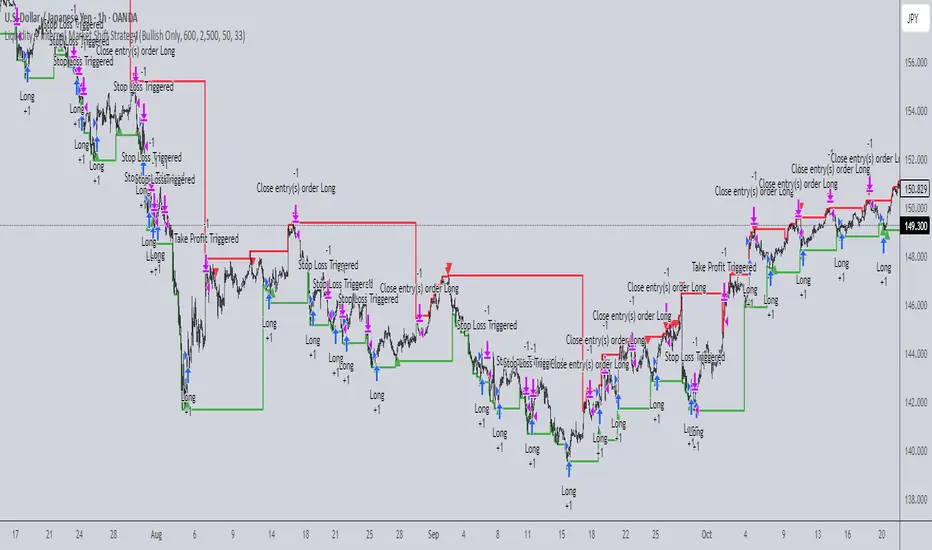
Liquidity + Internal Market Shift StrategyLiquidity + Internal Market Shift Strategy
This strategy combines liquidity zone analysis with the internal market structure, aiming to identify high-probability entry points. It uses key liquidity levels (local highs and lows) to track the price's interaction with significant market levels and then employs internal market shifts to trigger trades.
Key Features:
Internal Shift Logic: Instead of relying on traditional candlestick patterns like engulfing candles, this strategy utilizes internal market shifts. A bullish shift occurs when the price breaks previous bearish levels, and a bearish shift happens when the price breaks previous bullish levels, indicating a change in market direction.
Liquidity Zones: The strategy dynamically identifies key liquidity zones (local highs and lows) to detect potential reversal points and prevent trades in weak market conditions.
Mode Options: You can choose to run the strategy in "Both," "Bullish Only," or "Bearish Only" modes, allowing for flexibility based on market conditions.
Stop-Loss and Take-Profit: Customizable stop-loss and take-profit levels are integrated to manage risk and lock in profits.
Time Range Control: You can specify the time range for trading, ensuring the strategy only operates during the desired period.
This strategy is ideal for traders who want to combine liquidity analysis with internal structure shifts for precise market entries and exits.
This description clearly outlines the strategy's logic, the flexibility it provides, and how it works. You can adjust it further to match your personal trading style or preferences!
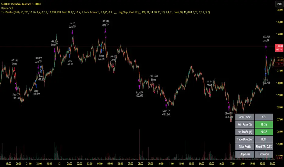
Trend Hunter Scalping [Daddin Algo]Trend Hunter Scalping Strategy Description
This strategy is a comprehensive scalping system designed to capture high-frequency trading opportunities within short timeframes. It combines multiple technical indicators to assess trend direction, momentum, volatility, and volume dynamics. Importantly, all parameters are user-adjustable, allowing the strategy to be optimized for various market conditions and individual preferences.
Technical Indicators and Settings
EMA (Exponential Moving Average):
The EMA is calculated based on a user-defined period. Rather than being fixed (e.g., a 200-period EMA), the period is adjustable to suit different market conditions. The position of the price relative to the EMA helps confirm the overall trend.
RSI & RSIOver:
The Relative Strength Index (RSI) measures momentum and the speed of price changes. Entry signals are generated when the RSI crosses its moving average. Additionally, overbought and oversold thresholds (set by the user) add an extra layer of confirmation for the signals.
ADX:
The Average Directional Index (ADX) assesses the strength of the current trend. When the ADX is above a user-specified threshold, the signals are considered more reliable. This helps in filtering out signals during weak trending periods.
Bollinger Bands:
Bollinger Bands gauge market volatility. The settings—including the length and the multiplier—are adjustable, providing flexibility to accommodate tightening or expanding volatility conditions.
Parabolic SAR:
This indicator identifies dynamic support and resistance levels, confirming the trend direction and helping pinpoint potential entry and exit points.
Pivot Levels (Fibonacci):
Calculated from the previous period's high, low, and close, pivot points and Fibonacci levels indicate potential reversal points and serve as support and resistance levels. These levels provide context for setting trailing stops and managing risk.
Volume Filter:
A volume condition ensures that trading signals are only considered valid when the current volume exceeds a multiple of its short-term moving average. This filter is adjustable, helping to confirm the strength of the market move.
Daddin Line:
Derived from a short-term moving average of the closing prices with a user-defined offset, the Daddin Line acts as an additional confirmation tool. Its parameters can be customized to better align with specific trading environments.
Trading Logic and Management
Signal Direction and Entry:
The strategy can generate both long (buy) and short (sell) signals, or be limited to one direction based on user preference. Entry orders are executed when all the selected indicator conditions are met. Additionally, maximum consecutive trade limits are implemented to help control risk.
Exit & Take Profit:
Trades are exited automatically when a user-defined profit percentage is reached. This take-profit percentage is flexible, enabling adjustments to match different market conditions or trading goals.
Trailing Stop (Dynamic Stop Loss):
A trailing stop mechanism is implemented using Fibonacci pivot levels. Once a position is open, the stop loss is dynamically updated as the price moves favorably. This ensures that profits are protected while minimizing losses in case of a sudden reversal.
Additional Features and Backtesting
Time Filtering (Backtesting):
The strategy includes a date range filter for backtesting. Users can define the start and end dates to evaluate the strategy’s performance during specific market periods, making it easier to assess its historical effectiveness.
Customizable Parameters:
Every indicator and risk management setting is fully customizable. This adaptability allows traders to tailor the strategy to different assets, timeframes, and market environments, ensuring optimal performance across diverse trading scenarios.
Conclusion
The Trend Hunter Scalping strategy effectively integrates multiple technical indicators to validate trends and manage risks efficiently. Its highly flexible, user-adjustable parameters make it adaptable to varying market conditions, providing traders with a robust framework for capturing quick trading opportunities.This strategy is designed to optimize both entry and exit points while offering comprehensive risk management controls.
IU BBB(Big Body Bar) StrategyDESCRIPTION
The IU BBB (Big Body Bar) Strategy is a price action-based trading strategy that identifies high-momentum candles with significantly larger body sizes compared to the average. It enters trades when a strong bullish or bearish move occurs and manages risk using an ATR-based trailing stop-loss system.
USER INPUTS:
- Big Body Threshold – Defines how many times larger the candle body should be compared to the average body ( default is 4 ).
- ATR Length – The period for the Average True Range (ATR) used in the trailing stop-loss calculation ( default is 14 ).
- ATR Factor – Multiplier for ATR to determine the trailing stop distance ( default is 2 ).
LONG CONDITION:
- The current candle’s body is greater than the average body size multiplied by the Big Body Threshold.
- The closing price is higher than the opening price (bullish candle).
SHORT CONDITION:
- The current candle’s body is greater than the average body size multiplied by the Big Body Threshold.
- The closing price is lower than the opening price (bearish candle).
LONG EXIT:
- ATR-based trailing stop-loss dynamically adjusts, locking in profits as the price moves higher.
SHORT EXIT:
- ATR-based trailing stop-loss dynamically adjusts, securing profits as the price moves lower.
WHY IT IS UNIQUE:
- Unlike traditional momentum strategies, this system adapts to volatility by filtering trades based on relative candle size.
- It incorporates an ATR-based trailing stop-loss, ensuring risk management and profit protection.
- The strategy avoids choppy market conditions by only trading when significant momentum is present.
HOW USERS CAN BENEFIT FROM IT:
- Catch Strong Price Moves – The strategy helps traders enter trades when the market shows decisive momentum.
- Effective Risk Management – The ATR-based trailing stop ensures that winning trades remain profitable.
- Works Across Markets – Can be applied to stocks, forex, crypto, and indices with proper optimization.
- Fully Customizable – Users can adjust sensitivity settings to match their trading style and time frame.

Simple APF Strategy Backtesting [The Quant Science]Simple backtesting strategy for the quantitative indicator Autocorrelation Price Forecasting. This is a Buy & Sell strategy that operates exclusively with long orders. It opens long positions and generates profit based on the future price forecast provided by the indicator. It's particularly suitable for trend-following trading strategies or directional markets with an established trend.
Main functions
1. Cycle Detection: Utilize autocorrelation to identify repetitive market behaviors and cycles.
2. Forecasting for Backtesting: Simulate trades and assess the profitability of various strategies based on future price predictions.
Logic
The strategy works as follow:
Entry Condition: Go long if the hypothetical gain exceeds the threshold gain (configurable by user interface).
Position Management: Sets a take-profit level based on the future price.
Position Sizing: Automatically calculates the order size as a percentage of the equity.
No Stop-Loss: this strategy doesn't includes any stop loss.
Example Use Case
A trader analyzes a dayli period using 7 historical bars for autocorrelation.
Sets a threshold gain of 20 points using a 5% of the equity for each trade.
Evaluates the effectiveness of a long-only strategy in this period to assess its profitability and risk-adjusted performance.
User Interface
Length: Set the length of the data used in the autocorrelation price forecasting model.
Thresold Gain: Minimum value to be considered for opening trades based on future price forecast.
Order Size: percentage size of the equity used for each single trade.
Strategy Limit
This strategy does not use a stop loss. If the price continues to drop and the future price forecast is incorrect, the trader may incur a loss or have their capital locked in the losing trade.
Disclaimer!
This is a simple template. Use the code as a starting point rather than a finished solution. The script does not include important parameters, so use it solely for educational purposes or as a boilerplate.

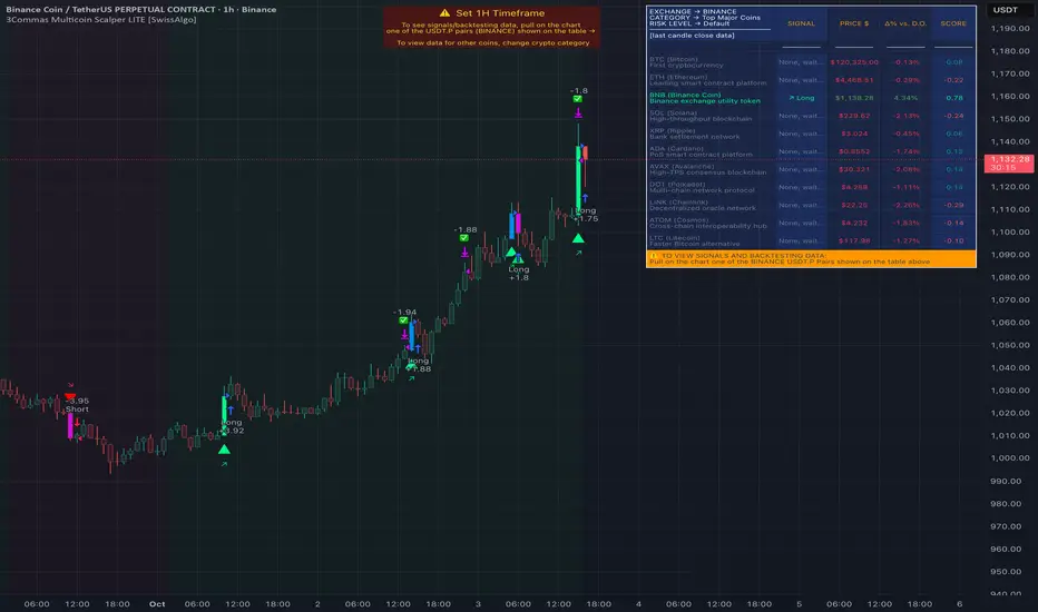
3Commas Multicoin Scalper LITE [SwissAlgo]
Introduction
Are you tired of tracking cryptocurrency charts and placing orders manually on your Exchange?
The 3Commas Multicoin Scalper LITE is an automated trading system designed to identify and execute potential trading setups on multiple cryptocurrencies ( simultaneously ) on your preferred Exchange (Binance, Bybit, OKX, Gate.io, Bitget) via 3Commas integration.
It analyzes price action, volume, momentum, volatility, and trend patterns across two categories of USDT Perpetual coins: the 'Top Major Coins' category (11 established cryptocurrencies) and your Custom Category (up to 10 coins of your choice).
The indicator sends real-time trading signals directly to your 3Commas bots for automated execution, identifying both trend-following and contrarian trading opportunities in all market conditions.
Trade automatically all coins of one or more selected categories:
----------------------------------------------
What it Does
The 3Commas Multicoin Scalper LITE is a technical analysis tool that monitors multiple cryptocurrency pairs simultaneously and connects with 3Commas for signal delivery and execution.
Here's how the strategy works:
🔶 Technical Analysis : Analyzes price action, volume, momentum, volatility, and trend patterns across USDT Perpetual Futures contracts simultaneously.
🔶 Pattern Detection : Identifies specific candle patterns and technical confluences that suggest potential trading setups across USDT.P contracts of the selected category.
🔶 Signal Generation : When technical criteria are met at bar close, the indicator creates deal-start signals for the relevant pairs.
🔶 3Commas Integration : Packages these signals and delivers them to 3Commas through TradingView alerts, allowing 3Commas bots to receive specific pair information ('Deal-Start' signals).
🔶 Category Management : Each TradingView alert monitors an entire category, allowing selective activation of different crypto categories.
🔶 Visual Feedback : Provides color-coded candles and backgrounds to visualize technical conditions, with optional pivot points and trend visualization.
Candle types
Signals
----------------------------------------------
Quick Start Guide
1. Setup 3Commas Bots : Configure two DCA bots in 3Commas (All USDT pairs) - one for LONG positions and one for SHORT positions.
2. Define Trading Parameters : Set your budget for each trade and adjust your preferred sensitivity within the indicator settings.
3. Create Category Alerts : Set up one TradingView alert for each crypto category you want to trade.
That's it! Once configured, the system automatically sends signals to your 3Commas bots when predefined trading setups are detected across coins in your selected/activated categories. The indicator scans all coins at bar close (for example, every hour on the 1H timeframe) and triggers trade execution only for those showing technical confluences.
Important : Consider your total capital when enabling categories. More details about the setup process are provided below (see paragraph "Detailed Setup & Configuration").
----------------------------------------------
Built-in Backtesting
The 3Commas Multicoin Scalper LITE includes backtesting visualization for each coin. When viewing any USDT Perpetual pair on your chart, you can visualize how the strategy would have performed historically on that specific asset.
Color-coded candles and signal markers show past trading setups, helping you evaluate which coins responded best to the strategy. This built-in backtesting capability can support your selection of assets/categories to trade before deploying real capital.
As backtesting results are hypothetical and do not guarantee future performance, your research and analysis are essential for selecting the crypto categories/coins to trade.
The default strategy settings are: Start Capital 1,000$, leverage 10X, Commissions 0.1% (average Taker Fee on Exchanges for average users), Order Amount 200$ for Longs/Shorts, Slippage 4
Example of backtesting view
----------------------------------------------
Key Features
🔶 Multi-Exchange Support : Compatible with BINANCE, BYBIT, BITGET, GATEIO, and OKX USDT Perpetual markets (USDT.P)
🔶 Category Options : Analyze cryptocurrencies in the Top Major Coins category or create your custom watchlist
🔶 Custom Category Option : Create your watchlist with up to 10 custom USDT Perpetual pairs
🔶 3Commas Integration : Seamlessly connects with 3Commas bots to automate trade entries and exits
🔶 Dual Strategy Approach : Identifies both "trend following" and "contrarian" potential setups
🔶 Confluence-Based Signals : Uses a combination of multiple technical factors - price spikes, price momentum, volume spikes, volume momentum, trend analysis, and volatility spikes - to generate potential trading setups
🔶 Risk Management : Adjustable sensitivity/risk levels, leverage settings, and budget allocation for each trade
🔶 Visual Indicators : Color-coded candles and trading signals provide visual feedback on market conditions
🔶 Trend Indication : Background colors showing ongoing uptrends/downtrends
🔶 Pivot Points & Daily Open : Optional display of pivot points and daily open price for additional context
🔶 Liquidity Analysis : Optional display of high/low liquidity timeframes throughout the trading week
🔶 Trade Control : Configurable limit for the maximum number of signals sent to 3Commas for execution (per bar close and category)
5 Available Exchanges
Pick coins/tokens and defined your Custom Category
----------------------------------------------
Methodology
The 3Commas Multicoin Scalper LITE utilizes a multi-faceted approach to identify potential trading setups:
1. Price Action Analysis : Detects abnormal price movements by comparing the current candle's range to historical averages and standard deviations, helping identify potential "pump and dump" scenarios or new-trends start
2. Price Momentum : Evaluates the relative strength of bullish vs. bearish price movements over time, indicating the build-up of buying or selling pressure.
3. Volume Analysis: Identifies unusual volume spikes by comparing current volume to historical averages, signaling strong market interest in a particular direction.
4. Volume Momentum : Measures the ratio of bullish to bearish volume, revealing the dominance of buyers or sellers over time.
5. Trend Analysis : Combines EMA slopes, RSI, and Stochastic RSI to determine overall trend direction and strength.
6. Volatility : Monitors the ATR (Average True Range) to detect periods of increased market volatility, which may indicate potential breakouts or reversals
7. Candle Wick Analysis : Evaluates upper and lower wick percentages to detect potential rejection patterns and reversals.
8. Pivot Point Analysis : Uses pivot points (PP, R1-R3, S1-S3) for identifying key support/resistance areas and potential breakout/breakdown levels.
9. Daily Open Reference: Analyzes price action relative to the daily open for potential setups related to price movement vs. the opening price
10. Market Timing/Liquidity : Evaluates high/low liquidity periods, specific days/times of heightened risk, and potential market manipulation timeframes.
11. Boost Factors : Applies additional weight to certain confluence patterns to adjust global scores
These factors are combined into a "Global Score" ranging from -1 to +1 , applied at bar close to the newly formed candles.
Scores above predefined thresholds (configurable via the Sensitivity Settings) indicate strong bullish or bearish conditions and trigger signals based on predefined patterns. The indicator then applies additional filters to generate specific "Trend Following" and "Contrarian" trading signals. The identified signals are packaged and sent to 3Commas for execution.
Pivot Points
Trend Background
----------------------------------------------
Who This Strategy Is For
The 3Commas Multicoin Scalper LITE may benefit:
Crypto Traders seeking to automate their trading across multiple coins simultaneously
3Commas Users looking to enhance their bot performance with technical signals
Busy Traders who want to monitor market opportunities without constant chart-watching
Multi-strategy traders interested in both trend-following and reversal trading approaches
Traders of Various Experience Levels from intermediate traders wanting to save time to advanced traders seeking to optimize their operations
Perpetual Futures Traders on major exchanges (Binance, Bybit, OKX, Gate.io, Bitget)
Swing and Scalp Traders seeking to identify short to medium-term profit opportunities
----------------------------------------------
Visual Indicators
The indicator provides visual feedback through:
1. Candlestick Colors :
* Lime: Strong bullish candle (High positive score)
* Blue: Moderate bullish candle (Medium positive score)
* Red: Strong bearish candle (High negative score)
* Purple: Moderate bearish candle (Medium negative score)
* Pale Green/Red: Mild bullish/bearish candle
2. Signal Markers :
* ↗: Trend following Long signal
* ↘: Trend following Short signal
* ⤴: Contrarian Long signal
* ⤵: Contrarian Short signal
3. Optional Elements :
* Pivot Points: Daily support/resistance levels (R1-R3, S1-S3, PP)
* Daily Open: Reference price level for the current trading day
* Trend Background: Color-coded background suggesting potential ongoing uptrend/downtrend
* Liquidity Highlighting: Background colors indicating typical high/low market liquidity periods
4. TradingView Strategy Plots and Backtesting Data : Standard performance metrics showing entry/exit points, equity curves, and trade statistics, based on the signals generated by the script.
----------------------------------------------
Detailed Setup & Configuration
The indicator features a user-friendly input panel organized in sequential steps to guide you through the complete setup process. Tooltips for each step provide additional information to help you understand the actions required to get the strategy running.
Informative tables provide additional details and instructions for critical setup steps such as 3Commas bot configuration and TradingView alert creation (to activate trading on specific categories).
1. Choose Exchange, Crypto Category & Sensitivity
* Select your USDT Perpetual Exchange (BINANCE, BYBIT, BITGET, GATEIO, or OKX) - i.e. the same Exchange connected in your 3Commas account
* Choose your preferred crypto category, or define your watchlist
* Choose from three sensitivity levels: Default, Aggressive, or Test Mode (test mode is designed to generate more signals, a potentially helpful feature when you are testing the indicator and alerts)
2. Setup 3Commas Bots and integrate them with the algo
* Create both LONG and SHORT DCA Bots in 3Commas
* Configure bots to accept signals for 'All USDT Pairs' with "TradingView Custom Signal" as deal start condition
* Enter your Bot IDs and Email Token in the indicator settings
* Set a maximum budget for LONG and SHORT trades
* Choose whether to allow LONG trades, SHORT trades, or both, according to your preference and market analysis
* Set maximum trades per bar/category (i.e. the max. number of simultaneous signals that the algo may send to your 3Commas bots for execution at every bar close - every hour if you set the 1H timeframe)
* Access the detailed setup guide table for step-by-step 3Commas configuration instructions
3Commas integration
3. Choose Visuals
* Toggle various optional visual elements to add to the chart: category metrics, fired alerts, coin metrics, daily open, pivot points
* Select a color theme: Dark or Light
4. Activate Trading via Alerts
* Create TradingView alerts for each category you want to trade
* Set alert condition to "3Commas Multicoin Scalper" with "Any alert() function call"
* Set the content of the message field to: {{Message}}, deleting the default content shown in this text field, to enable proper 3Commas integration (any other text than {{Message}}, would break the delivery trading signals from Tradingview to 3Commas)
* View the alerts setup instruction table for visual guidance on this critical step
Alerts
Fired Alerts (example at a single bar)
Fired Alerts (frequency)
Important Configuration Notes
Ensure that the TradingView chart's exchange matches your selected exchange in the indicator settings and your 3Commas bot settings.
You must configure the same leverage in both the script and your 3Commas bots
Your 3Commas bots must be configured for All USDT pairs
You must enter the exact Bot IDs and Email Token from 3Commas (these remain confidential - no one, including us, has access to them)
If you activate multiple categories without sufficient capital, 3Commas will display " insufficient funds " errors - align your available capital with the number of categories you activate (each deal will use the budget amount specified in user inputs)
You are free to set your Take Profit % / trailing on 3Commas
We recommend not to use DCA orders (i.e. set the number of DCA orders at zero)
Legend of symbols and plots on the chart
----------------------------------------------
FAQs
General Questions
❓ Q: What features are included in this indicator? A: This indicator provides access to the "Top Major Coins" category and a custom category option where you can define up to 10 pairs of your choice. It includes multi-exchange support, 3Commas integration, a dual strategy approach, visual indicators, trade controls, and comprehensive backtesting capabilities. The indicator is optimized to manage up to 2 trades per hour/category with leverage up to 10x and trade sizes up to 500 USDT - everything needed for traders looking to automate their crypto trading across multiple pairs simultaneously.
❓ Q: What is Global Score? A: The Global Score serves as a foundation for signal generation. When a candle's score exceeds certain thresholds (defined by your Risk Level setting), it becomes a candidate for signal generation. However, not all high-scoring candles generate trading signals - the indicator applies additional pattern recognition and contextual filters. For example, a strongly positive score (lime candle) in an established uptrend may trigger a "Trend Following" signal, while a strongly negative score (red candle) in a downtrend might generate a "Trend following Short" signal. Similarly, contrarian signals are generated when specific reversal patterns occur alongside appropriate Global Score values, often involving wick analysis and pivot point interactions. This multi-layer approach helps filter out false positives and identify higher-probability trading setups.
❓ Q: What's the difference between "Trend following" and "Contrarian" signals in the script? A: "Trend Following" signals follow the identified trends while "Contrarian" signals anticipate potential trend reversals.
❓ Q: Why don't I see any signals on my chart? A: Make sure you're viewing a USDT Perpetual pair from your selected exchange that belongs to the crypto category you've chosen to analyze. For example, if you've selected the "Top Major Coins" category with Binance as your exchange, you need to view a chart of one of those specific pairs (like BINANCE:BTCUSDT.P) to see signals. If you switch exchanges, for example from Binance to Bybit, you need to pull a Bybit pair on the chart to see backtesting data and signals.
❓ Q: Does this indicator guarantee profits? A: No. Trading cryptocurrencies involves significant risk, and past performance is not indicative of future results. This indicator is a tool to help you identify potential trading setups, but it does not and cannot guarantee profits.
❓ Q: Does this indicator repaint or use lookahead bias? A: No. All trading signals generated by this indicator are based only on completed price data and do not repaint. The system is designed to ensure that backtesting results reflect as closely as possible what you should experience in live trading.
While reference levels like pivot points are kept stable throughout the day using lookahead on, the actual buy and sell signals are calculated using only historical data (lookahead off) that would have been available at that moment in time. This ensures reliability and consistency between backtesting and real-time trading performance.
Technical Setup
❓ Q: What exchanges are supported? A: The strategy supports BINANCE, BYBIT, BITGET, GATEIO, and OKX USDT Perpetual markets (i.e. all the Exchanges you can connect to your 3Commas account for USDT Perpetual trading, excluding Coinbase Perpetual that offers USDC pairs, instead of USDT).
❓ Q: What timeframe should I use? A: The indicator is optimized for the 1-hour (1H) timeframe but may run on any timeframe.
❓ Q: How many coins can I trade at once? A: You can trade all coins within the selected category. You can activate categories by setting up alerts.
❓ Q: How many alerts do I need to set up? A: You need to set up one alert for each crypto category you want to trade. We recommend starting with one category, testing the results carefully, monitoring performance daily, and perhaps activating additional categories in a second stage.
❓ Q: Are there any specific risk management features built into the indicator? A: Yes, the indicator includes risk management features: adjustable maximum trades per hour/category, the ability to enable/disable long or short signals depending on market conditions, customizable trade size for both long and short positions, and different sensitivity/risk level settings.
❓ Q: What happens if 3Commas can't execute a signal? A: If 3Commas cannot execute a signal (due to insufficient funds, bot offline, etc.), the trade will be skipped. The indicator will continue sending signals for other valid setups, but it doesn't retry failed signals.
❓ Q: Can I run this indicator on multiple charts at once? A: Yes, but it's not necessary. The indicator analyzes all coins in your selected categories regardless of which chart you apply it to. For optimal resource usage, apply it to a single chart of a USDT Perpetual pair from your selected exchange. To stop trading a category, simply delete the alert created for that category.
❓ Q: How frequently does the indicator scan for new signals? A: The indicator scans all coins in your selected categories at the close of each bar (every hour if you selected the 1H timeframe).
----------------------------------------------
⚠️
Disclaimer
This indicator is for informational and educational purposes only and does not constitute financial advice. Trading cryptocurrencies involves significant risk, including the potential loss of all invested capital, and past performance is not indicative of future results.
Always conduct your own thorough research (DYOR) and understand the risks involved before making any trading decisions. Trading with leverage significantly amplifies both potential profits and losses - exercise extreme caution when using leverage and never risk more than you can afford to lose.
The Bot ID and Email Token information are transmitted directly from TradingView to 3Commas via secure connections. No third party or entity will ever have access to this data (including the Author). Do not share your 3Commas credentials with anyone.
This indicator is not affiliated with, endorsed by, or sponsored by TradingView or 3Commas.
3Commas Multicoin Scalper PRO [SwissAlgo]Introduction
Are you tired of tracking dozens of cryptocurrency charts and placing orders manually on your Exchange?
The 3Commas Multicoin Scalper PRO is an automated trading system designed to simultaneously identify and execute potential trading setups on multiple cryptocurrencies on your preferred Exchange (Binance, Bybit, OKX, Gate.io, Bitget) via 3Commas integration.
It analyzes price action, volume, momentum, volatility, and trend patterns across 180+ USDT Perpetual coins divided into 17 crypto categories , providing real-time signals directly to your 3Commas bots for automated trade execution. This indicator aims to identify potential trend-following and contrarian setups in both bull and bear markets.
-------------------------------------
What it Does
The 3Commas Multicoin Scalper PRO is a technical analysis tool that monitors multiple cryptocurrency pairs simultaneously and connects with 3Commas for signal delivery and execution.
Here's how the strategy works:
🔶 Technical Analysis : Analyzes price action, volume, momentum, volatility, and trend patterns across multiple USDT Perpetual Futures contracts simultaneously.
🔶 Pattern Detection : Identifies specific candle patterns and technical confluences that suggest potential trading setups across all USDT.P contracts of the selected categories
🔶 Signal Generation : When technical criteria are met at bar close, the indicator creates deal-start signals for the relevant pairs.
🔶 3Commas Integration : Packages these signals and delivers them to 3Commas through TradingView alerts, allowing 3Commas bots to receive specific pair information ('Deal-Start' signals).
🔶 Category Management : Each TradingView alert monitors an entire category (approximately 11 pairs), allowing selective activation of different crypto categories.
🔶 Visual Feedback : Provides color-coded candles and backgrounds to visualize technical conditions, with optional pivot points and trend visualization.
Candle types:
Signals:
-------------------------------------
Quick Start Guide
1. Setup 3Commas Bots : Configure two DCA bots in 3Commas (All USDT pairs) - one for LONG positions and one for SHORT positions.
2. Define Trading Parameters : Set your budget for each trade and adjust your preferred sensitivity within the indicator settings.
3. Create Category Alerts : Set up one TradingView alert for each crypto category you want to trade.
That's it! Once configured, the system automatically sends signals to your 3Commas bots when predefined trading setups are detected across coins in your selected/activated categories. The indicator scans all coins at bar close (for example, every hour on the 1H timeframe) and triggers trade execution only for those showing technical confluences.
Important : The more categories you activate by setting TradingView alerts, the more signals your 3Commas bots will receive. Consider your total capital when enabling multiple categories. More details about the setup process are provided below (see paragraph "Detailed Setup & Configuration")
-------------------------------------
Built-in Backtesting
The 3Commas Multicoin Scalper PRO includes backtesting visualization for each coin. When viewing any USDT Perpetual pair on your chart, you can visualize how the strategy would have performed historically on that specific asset.
Color-coded candles and signal markers show past trading setups, helping you evaluate which coins responded best to the strategy. This built-in backtesting capability can support your selection of assets/categories to trade before deploying real capital.
As backtesting results are hypothetical and do not guarantee future performance, your research and analysis are essential for selecting the crypto categories/coins to trade.
The default strategy settings are: Start Capital 1.000$, leverage 25X, Commissions 0.1% (average Taker Fee on Exchanges for average users), Order Amount 200$ for Longs/150$ for Shorts, Slippage 4
-------------------------------------
Key Features
🔶 Multi-Exchange Support : Compatible with BINANCE, BYBIT, BITGET, GATEIO, and OKX USDT Perpetual markets (USDT.P)
🔶 Wide Asset Coverage : Simultaneously analyzes 180+ cryptocurrencies across 17 specialized crypto categories
🔶 Custom Category Option : Create your watchlist with up to 10 custom USDT Perpetual pairs
🔶 3Commas Integration : Seamlessly connects with 3Commas bots to automate trade entries and exits
🔶 Dual Strategy Approach : Identifies both "trend following" and "contrarian" potential setups
🔶 Confluence-Based Signals : Uses a combination of multiple technical factors - price spikes, price momentum, volume spikes, volume momentum, trend analysis, and volatility spikes - to generate potential trading setups
🔶 Risk Management : Adjustable sensitivity/risk levels, leverage settings, and budget allocation for each trade
🔶 Visual Indicators : Color-coded candles and trading signals provide visual feedback on market conditions
🔶 Trend Indication : Background colors showing ongoing uptrends/downtrends
🔶 Pivot Points & Daily Open : Optional display of pivot points and daily open price for additional context
🔶 Liquidity Analysis : Optional display of high/low liquidity timeframes throughout the trading week
🔶 Trade Control : Configurable limit for the maximum number of signals sent to 3Commas for execution (per bar close and category)
Available Exchanges
Categories
Custom Category
Trend following/contrarian signals
-------------------------------------
Methodology
The 3Commas Multicoin Scalper PRO utilizes a multi-faceted approach to identify potential trading setups:
1. Price Action Analysis : Detects abnormal price movements by comparing the current candle's range to historical averages and standard deviations, helping identify potential "pump and dump" scenarios or new-trends start
2. Price Momentum : Evaluates the relative strength of bullish vs. bearish price movements over time, indicating the build-up of buying or selling pressure.
3. Volume Analysis: Identifies unusual volume spikes by comparing current volume to historical averages, signaling strong market interest in a particular direction.
4. Volume Momentum : Measures the ratio of bullish to bearish volume, revealing the dominance of buyers or sellers over time.
5. Trend Analysis : Combines EMA slopes, RSI, and Stochastic RSI to determine overall trend direction and strength.
6. Volatility : Monitors the ATR (Average True Range) to detect periods of increased market volatility, which may indicate potential breakouts or reversals
7. Candle Wick Analysis : Evaluates upper and lower wick percentages to detect potential rejection patterns and reversals.
8. Pivot Point Analysis : Uses pivot points (PP, R1-R3, S1-S3) for identifying key support/resistance areas and potential breakout/breakdown levels.
9. Daily Open Reference: Analyzes price action relative to the daily open for potential setups related to price movement vs. the opening price
10. Market Timing/Liquidity : Evaluates high/low liquidity periods, specific days/times of heightened risk, and potential market manipulation timeframes.
11. Boost Factors : Applies additional weight to certain confluence patterns to adjust global scores
These factors are combined into a "Global Score" ranging from -1 to +1 , applied at bar close to the newly formed candles.
Scores above predefined thresholds (configurable via the Sensitivity Settings) indicate strong bullish or bearish conditions and trigger signals based on predefined patterns. The indicator then applies additional filters to generate specific "Trend Following" and "Contrarian" trading signals. The identified signals are packaged and sent to 3Commas for execution.
Pivot Points
Daily open
Market Trend
Liquidity patterns by weekday
-------------------------------------
Who This Strategy Is For?
The 3Commas Multicoin Scalper PRO may benefit:
Crypto Traders seeking to automate their trading across multiple coins simultaneously
3Commas Users looking to enhance their bot performance with advanced technical signals
Busy Traders who want to monitor many market opportunities without constant chart-watching
Multi-strategy traders interested in both trend-following and reversal trading approaches
Traders of Various Experience Levels from intermediate traders wanting to save time to advanced traders seeking to scale their operations
Perpetual Futures Traders on major exchanges (Binance, Bybit, OKX, Gate.io, Bitget)
Swing and Scalp Traders seeking to identify short to medium-term profit opportunities
-------------------------------------
Visual Indicators
The indicator provides visual feedback through:
1. Candlestick Colors :
* Lime: Strong bullish candle (High positive score)
* Blue: Moderate bullish candle (Medium positive score)
* Red: Strong bearish candle (High negative score)
* Purple: Moderate bearish candle (Medium negative score)
* Pale Green/Red: Mild bullish/bearish candle
2. Signal Markers :
* ↗: Trend Following Long signal
* ↘: Trend Following Short signal
* ⤴: Contrarian Long signal
* ⤵: Contrarian Short signal
3. Optional Elements :
* Pivot Points: Daily support/resistance levels (R1-R3, S1-S3, PP)
* Daily Open: Reference price level for the current trading day
* Trend Background: Color-coded background suggesting potential ongoing uptrend/downtrend
* Liquidity Highlighting: Background colors indicating typical high/low market liquidity periods
4. TradingView Strategy Plots and Backtesting Data : Standard performance metrics showing entry/exit points, equity curves, and trade statistics, based on the signals generated by the script.
-------------------------------------
Detailed Setup & Configuration
The indicator features a user-friendly input panel organized in sequential steps to guide you through the complete setup process. Tooltips for each step provide additional information to help you understand the actions required to get the strategy running.
Informative tables provide additional details and instructions for critical setup steps such as 3Commas bot configuration and TradingView alert creation (to activate trading on specific categories).
1. Choose Exchange, Crypto Category & Sensitivity
* Select your USDT Perpetual Exchange (BINANCE, BYBIT, BITGET, GATEIO, or OKX) - i.e. the same Exchange connected in your 3Commas account
* Browse and choose your preferred crypto category, or define your watchlist
* Choose from three sensitivity levels: Default, Aggressive, or Test Mode (test mode is designed to generate way more signals, a potentially helpful feature when you are testing the indicator and alerts)
2. Setup 3Commas Bots and integrate them with the algo
* Create both LONG and SHORT DCA Bots in 3Commas
* Configure bots to accept signals for 'All USDT Pairs' with "TradingView Custom Signal" as deal start condition
* Enter your Bot IDs and Email Token in the indicator settings
* Set a maximum budget for LONG and SHORT trades
* Choose whether to allow LONG trades, SHORT trades, or both, according to your preference and market analysis
* Set maximum trades per bar/category (i.e. the max. number of simultaneous signals that the algo may send to your 3Commas bots for execution at every bar close - every hour if you set the 1H timeframe)
* Access the detailed setup guide table for step-by-step 3Commas configuration instructions
3Commas integration
3. Choose Visuals
* Toggle various optional visual elements to add to the chart: category metrics, fired alerts, coin metrics, daily open, pivot points
* Select a color theme: Dark or Light
4. Activate Trading via Alerts
* Create TradingView alerts for each category you want to trade
* Set alert condition to "3Commas Multicoin Scalper" with "Any alert() function call"
* Set the content of the message filed to: {{Message}}, deleting the default content shown in this text field, to enable proper 3Commas integration (any other text than {{Message}}, would break the delivery trading signals from Tradingview to 3Commas)
* View the alerts setup instruction table for visual guidance on this critical step
Alerts
Fired Alerts
Important Configuration Notes
Ensure that the TradingView chart's exchange matches your selected exchange in the indicator settings and your 3Commas bot settings.
You must configure the same leverage in both the script and your 3Commas bots
Your 3Commas bots must be configured for All USDT pairs
You must enter the exact Bot IDs and Email Token from 3Commas (these remain confidential - no one, including us, has access to them)
If you activate multiple categories without sufficient capital, 3Commas will display " insufficient funds " errors - align your available capital with the number of categories you activate (each deal will use the budget amount specified in user inputs)
You are free to set your Take Profit % / trailing on 3Commas
We recommend not to use DCA orders (i.e. set the number of DCA orders at zero)
Legend of symbols
-------------------------------------
FAQs
General Questions
❓ Q: What is Global Score? A: The Global Score serves as a foundation for signal generation. When a candle's score exceeds certain thresholds (defined by your Risk Level setting), it becomes a candidate for signal generation. However, not all high-scoring candles generate trading signals - the indicator applies additional pattern recognition and contextual filters. For example, a strongly positive score (lime candle) in an established uptrend may trigger a "Trend Following" signal, while a strongly negative score (red candle) in a downtrend might generate a "Trend Following Short" signal. Similarly, contrarian signals are generated when specific reversal patterns occur alongside appropriate Global Score values, often involving wick analysis and pivot point interactions. This multi-layer approach helps filter out false positives and identify higher-probability trading setups.
❓ Q: What's the difference between "Trend following" and "Contrarian" signals in the script? A: "Trend Following" signals follow the identified trends while "Contrarian" signals anticipate potential trend reversals.
❓ Q: Why can't I configure all the parameters? A: We've designed the solution to be plug-and-play to prevent users from getting lost in endless configurations. The preset values have been tested against their trade-offs in terms of financial performance, average trade duration, and risk levels.
❓ Q: Why don't I see any signals on my chart? A: Make sure you're viewing a USDT Perpetual pair from your selected exchange that belongs to the crypto category you've chosen to analyze. For example, if you've selected the "Top Major Coins" category with Binance as your exchange, you need to view a chart of one of those specific pairs (like BINANCE:BTCUSDT.P) to see signals. If you switch exchanges, for example from Binance to Bybit, you need to pull a Bybit pair on the chart to see backtesting data and signals.
❓ Q: Does this indicator guarantee profits? A: No. Trading cryptocurrencies involves significant risk, and past performance is not indicative of future results. This indicator is a tool to help you identify potential trading setups, but it does not and cannot guarantee profits.
❓ Q: Does this indicator repaint or use lookahead bias? A: No. All trading signals generated by this indicator are based only on completed price data and do not repaint. The system is designed to ensure that backtesting results reflect as closely as possible what you should experience in live trading.
While reference levels like pivot points are kept stable throughout the day using lookahead on, the actual buy and sell signals are calculated using only historical data (lookahead off) that would have been available at that moment in time. This ensures reliability and consistency between backtesting and real-time trading performance.
Technical Setup
❓ Q: What exchanges are supported? A: The strategy supports BINANCE, BYBIT, BITGET, GATEIO, and OKX USDT Perpetual markets (i.e. all the Exchanges you can connect to your 3Commas account for USDT Perpetual trading, excluding Coinbase Perpetual that offers UDSC pairs, instead of USDT).
❓ Q: What timeframe should I use? A: The indicator is optimized for the 1-hour (1H) timeframe but may run on any timeframe.
❓ Q: How many coins can I trade at once? A: You can trade all coins within each selected category (up to 11 coins per category in standard categories). You can activate multiple categories by setting up multiple alerts.
❓ Q: How many alerts do I need to set up? A: You need to set up one alert for each crypto category you want to trade. For example, if you want to trade both the "Top Major Coins" and the "DeFi" categories, you'll need to create two separate alerts, one for each category. We recommend starting with one category, testing the results carefully, monitoring performance daily, and perhaps activating additional categories in a second stage.
❓ Q: Are there any specific risk management features built into the indicator? A: Yes, the indicator includes risk management features: adjustable maximum trades per hour/category, the ability to enable/disable long or short signals depending on market conditions, customizable trade size for both long and short positions, and different sensitivity/risk level settings.
❓ Q: What happens if 3Commas can't execute a signal? A: If 3Commas cannot execute a signal (due to insufficient funds, bot offline, etc.), the trade will be skipped. The indicator will continue sending signals for other valid setups, but it doesn't retry failed signals.
❓ Q: Can I run this indicator on multiple charts at once? A: Yes, but it's not necessary. The indicator analyzes all coins in your selected categories regardless of which chart you apply it to. For optimal resource usage, apply it to a single chart of a USDT Perpetual pair from your selected exchange. To stop trading a category delete the alert created for that category.
❓ Q: How frequently does the indicator scan for new signals? A: The indicator scans all coins in your selected categories at the close of each bar (every hour if you selected the 1H timeframe).
3Commas Integration
❓ Q: Do I need a 3Commas account? A: Yes, a 3Commas account with active DCA bots (both LONG and SHORT) is required for automated trade execution. A paid subscription is needed, as multipair Bots and multiple simultaneous deals are involved.
❓ Q: How do I set the leverage? A: Set the leverage identically in both the indicator settings and your 3Commas DCA bots (the max supported leverage is 50x). Always be careful about leverage, as it amplifies both profits and losses.
❓ Q: Where do I find my 3Commas Bot IDs and Email Token? A: Open your 3Commas DCA bot and scroll to the "Messages" section. You'll find the Bot ID and Email Token within any message (e.g., "Start Deal").
Display Settings
❓ Q: What does the Sensitivity setting do? A: It adjusts the sensitivity of signal generation. "Default" provides a balanced approach with moderate signal frequency. "Aggressive" lowers the thresholds for signal generation, potentially increasing trade frequency but may include more noise. "Test Mode" is the most sensitive setting, useful for testing alert configurations but not recommended for live trading. Higher risk levels may generate more signals but with potentially lower average quality, while lower risk levels produce fewer but potentially better signals.
❓ Q: What does "Show fired alerts" do? A: The "Show fired alerts" option displays a label on your chart showing which signals have been fired and sent to 3Commas during the most recent candle closes. This visual indicator helps you confirm that your alerts are working properly and shows which coins from your selected category have triggered signals. It's useful when setting up and testing the system, allowing you to verify that signals are being sent to 3Commas as expected and their frequency over time.
❓ Q: What does "Show coin/token metrics" do? A: This toggle displays detailed technical metrics for the specific coin/token currently shown on your chart. When enabled, it shows statistics for the last closed candle for that coin.
❓ Q: What does "Show most liquid days/times" do? A: This toggle displays color-coded background highlighting to indicate periods of varying market liquidity throughout the trading week. Green backgrounds show generally higher liquidity periods (typically weekday trading hours), yellow highlights potentially manipulative periods (often Sunday/Monday overnight), and gray indicates low liquidity periods (when major markets are closed or during late hours).
⚠️ Disclaimer
This indicator is for informational and educational purposes only and does not constitute financial advice. Trading cryptocurrencies involves significant risk, including the potential loss of all invested capital, and past performance is not indicative of future results.
Always conduct your own thorough research (DYOR) and understand the risks involved before making any trading decisions. Trading with leverage significantly amplifies both potential profits and losses - exercise extreme caution when using leverage and never risk more than you can afford to lose.
The Bot ID and Email Token information are transmitted directly from TradingView to 3Commas via secure connections. No third party or entity will ever have access to this data (including the Author). Do not share your 3Commas credentials with anyone.
This indicator is not affiliated with, endorsed by, or sponsored by TradingView or 3Commas.

[3Commas] Turtle StrategyTurtle Strategy
🔷 What it does: This indicator implements a modernized version of the Turtle Trading Strategy, designed for trend-following and automated trading with webhook integration. It identifies breakout opportunities using Donchian channels, providing entry and exit signals.
Channel 1: Detects short-term breakouts using the highest highs and lowest lows over a set period (default 20).
Channel 2: Acts as a confirmation filter by applying an offset to the same period, reducing false signals.
Exit Channel: Functions as a dynamic stop-loss (wait for candle close), adjusting based on market structure (default 10 periods).
Additionally, traders can enable a fixed Take Profit level, ensuring a systematic approach to profit-taking.
🔷 Who is it for:
Trend Traders: Those looking to capture long-term market moves.
Bot Users: Traders seeking to automate entries and exits with bot integration.
Rule-Based Traders: Operators who prefer a structured, systematic trading approach.
🔷 How does it work: The strategy generates buy and sell signals using a dual-channel confirmation system.
Long Entry: A buy signal is generated when the close price crosses above the previous high of Channel 1 and is confirmed by Channel 2.
Short Entry: A sell signal occurs when the close price falls below the previous low of Channel 1, with confirmation from Channel 2.
Exit Management: The Exit Channel acts as a trailing stop, dynamically adjusting to price movements. To exit the trade, wait for a full bar close.
Optional Take Profit (%): Closes trades at a predefined %.
🔷 Why it’s unique:
Modern Adaptation: Updates the classic Turtle Trading Strategy, with the possibility of using a second channel with an offset to filter the signals.
Dynamic Risk Management: Utilizes a trailing Exit Channel to help protect gains as trades move favorably.
Bot Integration: Automates trade execution through direct JSON signal communication with your DCA Bots.
🔷 Considerations Before Using the Indicator:
Market & Timeframe: Best suited for trending markets; higher timeframes (e.g., H4, D1) are recommended to minimize noise.
Sideways Markets: In choppy conditions, breakouts may lead to false signals—consider using additional filters.
Backtesting & Demo Testing: It is crucial to thoroughly backtest the strategy and run it on a demo account before risking real capital.
Parameter Adjustments: Ensure that commissions, slippage, and position sizes are set accurately to reflect real trading conditions.
🔷 STRATEGY PROPERTIES
Symbol: BINANCE:ETHUSDT (Spot).
Timeframe: 4h.
Test Period: All historical data available.
Initial Capital: 10000 USDT.
Order Size per Trade: 1% of Capital, you can use a higher value e.g. 5%, be cautious that the Max Drawdown does not exceed 10%, as it would indicate a very risky trading approach.
Commission: Binance commission 0.1%, adjust according to the exchange being used, lower numbers will generate unrealistic results. By using low values e.g. 5%, it allows us to adapt over time and check the functioning of the strategy.
Slippage: 5 ticks, for pairs with low liquidity or very large orders, this number should be increased as the order may not be filled at the desired level.
Margin for Long and Short Positions: 100%.
Indicator Settings: Default Configuration.
Period Channel 1: 20.
Period Channel 2: 20.
Period Channel 2 Offset: 20.
Period Exit: 10.
Take Profit %: Disable.
Strategy: Long & Short.
🔷 STRATEGY RESULTS
⚠️Remember, past results do not guarantee future performance.
Net Profit: +516.87 USDT (+5.17%).
Max Drawdown: -100.28 USDT (-0.95%).
Total Closed Trades: 281.
Percent Profitable: 40.21%.
Profit Factor: 1.704.
Average Trade: +1.84 USDT (+1.80%).
Average # Bars in Trades: 29.
🔷 How to Use It:
🔸 Adjust Settings:
Select your asset and timeframe suited for trend trading.
Adjust the periods for Channel 1, Channel 2, and the Exit Channel to align with the asset’s historical behavior. You can visualize these channels by going to the Style tab and enabling them.
For example, if you set Channel 2 to 40 with an offset of 40, signals will take longer to appear but will aim for a more defined trend.
Experiment with different values, a possible exit configuration is using 20 as well. Compare the results and adjust accordingly.
Enable the Take Profit (%) option if needed.
🔸Results Review:
It is important to check the Max Drawdown. This value should ideally not exceed 10% of your capital. Consider adjusting the trade size to ensure this threshold is not surpassed.
Remember to include the correct values for commission and slippage according to the symbol and exchange where you are conducting the tests. Otherwise, the results will not be realistic.
If you are satisfied with the results, you may consider automating your trades. However, it is strongly recommended to use a small amount of capital or a demo account to test proper execution before committing real funds.
🔸Create alerts to trigger the DCA Bot:
Verify Messages: Ensure the message matches the one specified by the DCA Bot.
Multi-Pair Configuration: For multi-pair setups, enable the option to add the symbol in the correct format.
Signal Settings: Enable the option to receive long or short signals (Entry | TP | SL), copy and paste the messages for the DCA Bots configured.
Alert Setup:
When creating an alert, set the condition to the indicator and choose "alert() function call only".
Enter any desired Alert Name.
Open the Notifications tab, enable Webhook URL, and paste the Webhook URL.
For more details, refer to the section: "How to use TradingView Custom Signals".
Finalize Alerts: Click Create, you're done! Alerts will now be sent automatically in the correct format.
🔷 INDICATOR SETTINGS
Period Channel 1: Period of highs and lows to trigger signals
Period Channel 2: Period of highs and lows to filter signals
Offset: Move Channel 2 to the right x bars to try to filter out the favorable signals.
Period Exit: It is the period of the Donchian channel that is used as trailing for the exits.
Strategy: Order Type direction in which trades are executed.
Take Profit %: When activated, the entered value will be used as the Take Profit in percentage from the entry price level.
Use Custom Test Period: When enabled signals only works in the selected time window. If disabled it will use all historical data available on the chart.
Test Start and End: Once the Custom Test Period is enabled, here you select the start and end date that you want to analyze.
Check Messages: Check Messages: Enable this option to review the messages that will be sent to the bot.
Entry | TP | SL: Enable this options to send Buy Entry, Take Profit (TP), and Stop Loss (SL) signals.
Deal Entry and Deal Exit: Copy and paste the message for the deal start signal and close order at Market Price of the DCA Bot. This is the message that will be sent with the alert to the Bot, you must verify that it is the same as the bot so that it can process properly.
DCA Bot Multi-Pair: You must activate it if you want to use the signals in a DCA Bot Multi-pair in the text box you must enter (using the correct format) the symbol in which you are creating the alert, you can check the format of each symbol when you create the bot.
👨🏻💻💭 We hope this tool helps enhance your trading. Your feedback is invaluable, so feel free to share any suggestions for improvements or new features you'd like to see implemented.
__
The information and publications within the 3Commas TradingView account are not meant to be and do not constitute financial, investment, trading, or other types of advice or recommendations supplied or endorsed by 3Commas and any of the parties acting on behalf of 3Commas, including its employees, contractors, ambassadors, etc.

FVG Breakout Lite by tradingbauhausExplanation of "FVG Breakout Lite by tradingbauhaus"
This script is a trading strategy built for TradingView that helps you spot and trade "Fair Value Gaps" (FVGs)—price areas where the market moved quickly, leaving a gap that might act as support or resistance later. It’s designed to catch breakout opportunities when the price moves strongly in one direction, with extra filters to make trades more reliable. Here’s how it works and how you can use it:
What It Does
1. Finds Fair Value Gaps (FVGs):
A "Bullish FVG" happens when the price jumps up quickly, leaving a gap below where it didn’t trade much (e.g., today’s low is higher than the high from two bars ago).
A "Bearish FVG" is the opposite: the price drops fast, leaving a gap above (e.g., today’s high is lower than the low from two bars ago).
The script draws colored boxes on your chart to show these gaps: green for bullish, red for bearish.
2. Spots Breakouts:
It looks for "strong" FVGs by comparing them to a trend (based on the highest highs and lowest lows over a set period).
If a bullish gap forms above the recent highs, or a bearish gap below the recent lows, it’s marked as a breakout opportunity.
3. Adds a Volume Check:
Trades only happen if the market’s volume is higher than usual (e.g., 1.2x the average volume over the last 20 bars). This helps ensure the breakout has real momentum behind it.
4. Trades Automatically:
Long Trades (Buy): If a bullish breakout FVG forms and volume is high, it buys at the current price.
Short Trades (Sell): If a bearish breakout FVG forms with high volume, it sells short.
Each trade comes with a stop loss (to limit losses) and a take profit (to lock in gains), both adjustable by you.
5. Shows Mitigation Lines (Optional):
If you turn on "Display Mitigation Zones," it draws lines at the edge of each breakout FVG. These lines show where the price might return to "fill" the gap later, helping you see key levels.
6. Includes Webull Costs:
The script factors in real trading fees from Webull, like tiny SEC and FINRA fees for selling, and a daily margin cost if you’re borrowing money to trade. These don’t show up on the chart but affect the strategy’s performance in backtesting.
How to Use It
1. Add to Your Chart:
Copy the script into TradingView’s Pine Editor, click "Add to Chart," and it’ll start drawing FVGs and running the strategy.
2. Customize Settings:
Trend Period (Default: 25): How many bars it looks back to define the trend. Longer periods mean fewer but stronger signals.
Volume Lookback (Default: 20) & Volume Threshold (Default: 1.2): Adjust how it measures "high volume." Increase the threshold for stricter trades.
Stop Loss % (Default: 1.5%) & Take Profit % (Default: 3%): Set how much you’re willing to lose or aim to gain per trade.
Margin Rate % (Default: 8.74%): Webull’s rate for borrowing money—lower it if your account qualifies for a better rate.
Display Mitigation Zones (Default: On): Toggle this to see or hide the gap lines.
Colors: Change the green (bullish) and red (bearish) shades to suit your chart.
3. Backtest It:
Go to the "Strategy Tester" tab in TradingView to see how it performs on past data. It’ll show trades, profits, losses, and Webull fees included.
4. Watch It Work:
Green boxes mean bullish FVGs; red boxes mean bearish FVGs. If volume spikes and the price breaks out, you’ll see trades happen automatically.
What to Expect
Visuals: You’ll see colored boxes for FVGs and optional lines showing where they start. These help you spot key price zones even if you’re not trading.
Trades: It’s selective—only trades when FVGs align with a breakout and volume confirms it. Expect fewer trades but with higher potential.
Risk: The stop loss keeps losses in check, while the take profit aims for a 2:1 reward-to-risk ratio by default (3% gain vs. 1.5% loss).
Costs: Webull’s fees are small but baked into the results, so you’re seeing a realistic picture of profits.
Tips for Users
Test it on a small timeframe (like 5-minute charts) for day trading or a larger one (like daily) for swing trading.
Play with the volume threshold—if you get too few trades, lower it (e.g., 1.1); if too many, raise it (e.g., 1.5).
Watch how price reacts to the mitigation lines—they’re often support or resistance zones traders target.
This strategy is lightweight, focused, and built for traders who like breakouts with a bit of confirmation. It’s not foolproof (no strategy is!), but it gives you a clear way to trade FVGs with some smart filters.
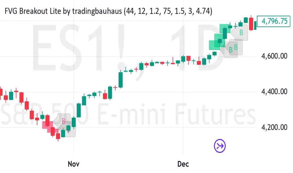
SuperTrend AI Oscillator StrategySuperTrend AI Oscillator Strategy
Overview
This strategy is a trend-following approach that combines the SuperTrend indicator with oscillator-based filtering.
By identifying market trends while utilizing oscillator-based momentum analysis, it aims to improve entry precision.
Additionally, it incorporates a trailing stop to strengthen risk management while maximizing profits.
This strategy can be applied to various markets, including Forex, Crypto, and Stocks, as well as different timeframes. However, its effectiveness varies depending on market conditions, so thorough testing is required.
Features
1️⃣ Trend Identification Using SuperTrend
The SuperTrend indicator (a volatility-adjusted trend indicator based on ATR) is used to determine trend direction.
A long entry is considered when SuperTrend turns bullish.
A short entry is considered when SuperTrend turns bearish.
The goal is to capture clear trend reversals and avoid unnecessary trades in ranging markets.
2️⃣ Entry Filtering with an Oscillator
The Super Oscillator is used to filter entry signals.
If the oscillator exceeds 50, it strengthens long entries (indicating strong bullish momentum).
If the oscillator drops below 50, it strengthens short entries (indicating strong bearish momentum).
This filter helps reduce trades in uncertain market conditions and improves entry accuracy.
3️⃣ Risk Management with a Trailing Stop
Instead of a fixed stop loss, a SuperTrend-based trailing stop is implemented.
The stop level adjusts automatically based on market volatility.
This allows profits to run while managing downside risk effectively.
4️⃣ Adjustable Risk-Reward Ratio
The default risk-reward ratio is set at 1:2.
Example: A 1% stop loss corresponds to a 2% take profit target.
The ratio can be customized according to the trader’s risk tolerance.
5️⃣ Clear Trade Signals & Visual Support
Green "BUY" labels indicate long entry signals.
Red "SELL" labels indicate short entry signals.
The Super Oscillator is plotted in a separate subwindow to visually assess trend strength.
A real-time trailing stop is displayed to support exit strategies.
These visual aids make it easier to identify entry and exit points.
Trading Parameters & Considerations
Initial Account Balance: Default is $7,000 (adjustable).
Base Currency: USD
Order Size: 10,000 USD
Pyramiding: 1
Trading Fees: $0.94 per trade
Long Position Margin: 50%
Short Position Margin: 50%
Total Trades (M5 Timeframe): 1,032
Visual Aids for Clarity
This strategy includes clear visual trade signals to enhance decision-making:
Green "BUY" labels for long entries
Red "SELL" labels for short entries
Super Oscillator plotted in a subwindow with a 50 midline
Dynamic trailing stop displayed for real-time trend tracking
These visual aids allow traders to quickly identify trade setups and manage positions with greater confidence.
Summary
The SuperTrend AI Oscillator Strategy is developed based on indicators from Black Cat and LuxAlgo.
By integrating high-precision trend analysis with AI-based oscillator filtering, it provides a strong risk-managed trading approach.
Important Notes
This strategy does not guarantee profits—performance varies based on market conditions.
Past performance does not guarantee future results. Markets are constantly changing.
Always test extensively with backtesting and demo trading before using it in live markets.
Risk management, position sizing, and market conditions should always be considered when trading.
Conclusion
This strategy combines trend analysis with momentum filtering, enhancing risk management in trading.
By following market trends carefully, making precise entries, and using trailing stops, it seeks to reduce risk while maximizing potential profits.
Before using this strategy, be sure to test it thoroughly via backtesting and demo trading, and adjust the settings to match your trading style.

Aggressive Strategy for High IV Market### Strategic background
In a volatile high IV market, prices are volatile and market expectations of future uncertainty are high. This environment provides opportunities for aggressive trading strategies, but also comes with a high level of risk. In pursuit of a high Sharpe ratio (i.e., risk-adjusted return), we need to design a strategy that captures the benefits of market volatility while effectively controlling risk. Based on daily line cycles, I choose a combination of trend tracking and volatility filtering for highly volatile assets such as stocks, futures or cryptocurrencies.
---
### Strategy framework
#### Data
- Use daily data, including opening, closing, high and low prices.
- Suitable for highly volatile markets such as technology stocks, cryptocurrencies or volatile index futures.
#### Core indicators
1. ** Trend Indicators ** :
Fast Exponential Moving Average (EMA_fast) : 10-day EMA, used to capture short-term trends.
- Slow Exponential Moving Average (EMA_slow) : 30-day EMA, used to determine the long-term trend.
2. ** Volatility Indicators ** :
Average true Volatility (ATR) : 14-day ATR, used to measure market volatility.
- ATR mean (ATR_mean) : A simple moving average of the 20-day ATR that serves as a volatility benchmark.
- ATR standard deviation (ATR_std) : The standard deviation of the 20-day ATR, which is used to judge extreme changes in volatility.
#### Trading logic
The strategy is based on a trend following approach of double moving averages and filters volatility through ATR indicators, ensuring that trading only in a high-volatility environment is in line with aggressive and high sharpe ratio goals.
---
### Entry and exit conditions
#### Admission conditions
- ** Multiple entry ** :
- EMA_fast Crosses EMA_slow (gold cross), indicating that the short-term trend is turning upward.
-ATR > ATR_mean + 1 * ATR_std indicates that the current volatility is above average and the market is in a state of high volatility.
- ** Short Entry ** :
- EMA_fast Crosses EMA_slow (dead cross) downward, indicating that the short-term trend turns downward.
-ATR > ATR_mean + 1 * ATR_std, confirming high volatility.
#### Appearance conditions
- ** Long show ** :
- EMA_fast Enters the EMA_slow (dead cross) downward, and the trend reverses.
- or ATR < ATR_mean-1 * ATR_std, volatility decreases significantly and the market calms down.
- ** Bear out ** :
- EMA_fast Crosses the EMA_slow (gold cross) on the top, and the trend reverses.
- or ATR < ATR_mean-1 * ATR_std, the volatility is reduced.
---
### Risk management
To control the high risk associated with aggressive strategies, set up the following mechanisms:
1. ** Stop loss ** :
- Long: Entry price - 2 * ATR.
- Short: Entry price + 2 * ATR.
- Dynamic stop loss based on ATR can adapt to market volatility changes.
2. ** Stop profit ** :
- Fixed profit target can be selected (e.g. entry price ± 4 * ATR).
- Or use trailing stop losses to lock in profits following price movements.
3. ** Location Management ** :
- Reduce positions appropriately in times of high volatility, such as dynamically adjusting position size according to ATR, ensuring that the risk of a single trade does not exceed 1%-2% of the account capital.
---
### Strategy features
- ** Aggressiveness ** : By trading only in a high ATR environment, the strategy takes full advantage of market volatility and pursues greater returns.
- ** High Sharpe ratio potential ** : Trend tracking combined with volatility filtering to avoid ineffective trades during periods of low volatility and improve the ratio of return to risk.
- ** Daily line Cycle ** : Based on daily line data, suitable for traders who operate frequently but are not too complex.
---
### Implementation steps
1. ** Data Preparation ** :
- Get the daily data of the target asset.
- Calculate EMA_fast (10 days), EMA_slow (30 days), ATR (14 days), ATR_mean (20 days), and ATR_std (20 days).
2. ** Signal generation ** :
- Check EMA cross signals and ATR conditions daily to generate long/short signals.
3. ** Execute trades ** :
- Enter according to the signal, set stop loss and profit.
- Monitor exit conditions and close positions in time.
4. ** Backtest and Optimization ** :
- Use historical data to backtest strategies to evaluate Sharpe ratios, maximum retracements, and win rates.
- Optimize parameters such as EMA period and ATR threshold to improve policy performance.
---
### Precautions
- ** Trading costs ** : Highly volatile markets may result in frequent trading, and the impact of fees and slippage on earnings needs to be considered.
- ** Risk Control ** : Aggressive strategies may face large retracements and need to strictly implement stop losses.
- ** Scalability ** : Additional metrics (such as volume or VIX) can be added to enhance strategy robustness, or combined with machine learning to predict trends and volatility.
---
### Summary
This is a trend following strategy based on dual moving averages and ATR, designed for volatile high IV markets. By entering into high volatility and exiting into low volatility, the strategy combines aggressive and risk-adjusted returns for traders seeking a high sharpe ratio. It is recommended to fully backtest before implementation and adjust the parameters according to the specific market.
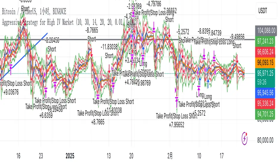
ADX for BTC [PineIndicators]The ADX Strategy for BTC is a trend-following system that uses the Average Directional Index (ADX) to determine market strength and momentum shifts. Designed for Bitcoin trading, this strategy applies a customizable ADX threshold to confirm trend signals and optionally filters entries using a Simple Moving Average (SMA). The system features automated entry and exit conditions, dynamic trade visualization, and built-in trade tracking for historical performance analysis.
⚙️ Core Strategy Components
1️⃣ Average Directional Index (ADX) Calculation
The ADX indicator measures trend strength without indicating direction. It is derived from the Positive Directional Movement (+DI) and Negative Directional Movement (-DI):
+DI (Positive Directional Index): Measures upward price movement.
-DI (Negative Directional Index): Measures downward price movement.
ADX Value: Higher values indicate stronger trends, regardless of direction.
This strategy uses a default ADX length of 14 to smooth out short-term fluctuations while detecting sustainable trends.
2️⃣ SMA Filter (Optional Trend Confirmation)
The strategy includes a 200-period SMA filter to validate trend direction before entering trades. If enabled:
✅ Long Entry is only allowed when price is above a long-term SMA multiplier (5x the standard SMA length).
✅ If disabled, the strategy only considers the ADX crossover threshold for trade entries.
This filter helps reduce entries in sideways or weak-trend conditions, improving signal reliability.
📌 Trade Logic & Conditions
🔹 Long Entry Conditions
A buy signal is triggered when:
✅ ADX crosses above the threshold (default = 14), indicating a strengthening trend.
✅ (If SMA filter is enabled) Price is above the long-term SMA multiplier.
🔻 Exit Conditions
A position is closed when:
✅ ADX crosses below the stop threshold (default = 45), signaling trend weakening.
By adjusting the entry and exit ADX levels, traders can fine-tune sensitivity to trend changes.
📏 Trade Visualization & Tracking
Trade Markers
"Buy" label (▲) appears when a long position is opened.
"Close" label (▼) appears when a position is exited.
Trade History Boxes
Green if a trade is profitable.
Red if a trade closes at a loss.
Trend Tracking Lines
Horizontal lines mark entry and exit prices.
A filled trade box visually represents trade duration and profitability.
These elements provide clear visual insights into trade execution and performance.
⚡ How to Use This Strategy
1️⃣ Apply the script to a BTC chart in TradingView.
2️⃣ Adjust ADX entry/exit levels based on trend sensitivity.
3️⃣ Enable or disable the SMA filter for trend confirmation.
4️⃣ Backtest performance to analyze historical trade execution.
5️⃣ Monitor trade markers and history boxes for real-time trend insights.
This strategy is designed for trend traders looking to capture high-momentum market conditions while filtering out weak trends.
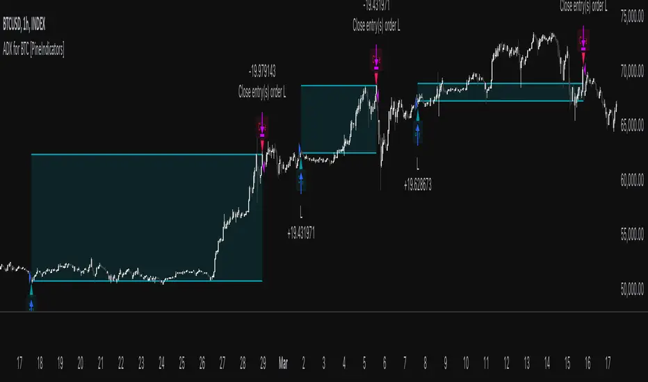
MACD Volume Strategy for XAUUSD (15m) [PineIndicators]The MACD Volume Strategy is a momentum-based trading system designed for XAUUSD on the 15-minute timeframe. It integrates two key market indicators: the Moving Average Convergence Divergence (MACD) and a volume-based oscillator to identify strong trend shifts and confirm trade opportunities. This strategy uses dynamic position sizing, incorporates leverage customization, and applies structured entry and exit conditions to improve risk management.
⚙️ Core Strategy Components
1️⃣ Volume-Based Momentum Calculation
The strategy includes a custom volume oscillator to filter trade signals based on market activity. The oscillator is derived from the difference between short-term and long-term volume trends using Exponential Moving Averages (EMAs)
Short EMA (default = 5) represents recent volume activity.
Long EMA (default = 8) captures broader volume trends.
Positive values indicate rising volume, supporting momentum-based trades.
Negative values suggest weak market activity, reducing signal reliability.
By requiring positive oscillator values, the strategy ensures momentum confirmation before entering trades.
2️⃣ MACD Trend Confirmation
The strategy uses the MACD indicator as a trend filter. The MACD is calculated as:
Fast EMA (16-period) detects short-term price trends.
Slow EMA (26-period) smooths out price fluctuations to define the overall trend.
Signal Line (9-period EMA) helps identify crossovers, signaling potential trend shifts.
Histogram (MACD – Signal) visualizes trend strength.
The system generates trade signals based on MACD crossovers around the zero line, confirming bullish or bearish trend shifts.
📌 Trade Logic & Conditions
🔹 Long Entry Conditions
A buy signal is triggered when all the following conditions are met:
✅ MACD crosses above 0, signaling bullish momentum.
✅ Volume oscillator is positive, confirming increased trading activity.
✅ Current volume is at least 50% of the previous candle’s volume, ensuring market participation.
🔻 Short Entry Conditions
A sell signal is generated when:
✅ MACD crosses below 0, indicating bearish momentum.
✅ Volume oscillator is positive, ensuring market activity is sufficient.
✅ Current volume is less than 50% of the previous candle’s volume, showing decreasing participation.
This multi-factor approach filters out weak or false signals, ensuring that trades align with both momentum and volume dynamics.
📏 Position Sizing & Leverage
Dynamic Position Calculation:
Qty = strategy.equity × leverage / close price
Leverage: Customizable (default = 1x), allowing traders to adjust risk exposure.
Adaptive Sizing: The strategy scales position sizes based on account equity and market price.
Slippage & Commission: Built-in slippage (2 points) and commission (0.01%) settings provide realistic backtesting results.
This ensures efficient capital allocation, preventing overexposure in volatile conditions.
🎯 Trade Management & Exits
Take Profit & Stop Loss Mechanism
Each position includes predefined profit and loss targets:
Take Profit: +10% of risk amount.
Stop Loss: Fixed at 10,100 points.
The risk-reward ratio remains balanced, aiming for controlled drawdowns while maximizing trade potential.
Visual Trade Tracking
To improve trade analysis, the strategy includes:
📌 Trade Markers:
"Buy" label when a long position opens.
"Close" label when a position exits.
📌 Trade History Boxes:
Green for profitable trades.
Red for losing trades.
📌 Horizontal Trade Lines:
Shows entry and exit prices.
Helps identify trend movements over multiple trades.
This structured visualization allows traders to analyze past performance directly on the chart.
⚡ How to Use This Strategy
1️⃣ Apply the script to a XAUUSD (Gold) 15m chart in TradingView.
2️⃣ Adjust leverage settings as needed.
3️⃣ Enable backtesting to assess past performance.
4️⃣ Monitor volume and MACD conditions to understand trade triggers.
5️⃣ Use the visual trade markers to review historical performance.
The MACD Volume Strategy is designed for short-term trading, aiming to capture momentum-driven opportunities while filtering out weak signals using volume confirmation.
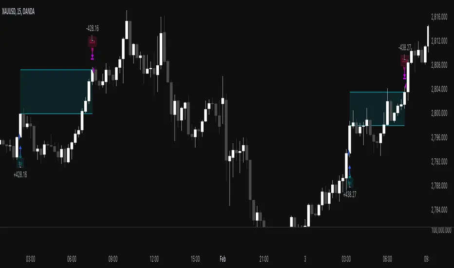
2xSPYTIPS Strategy by Fra public versionThis is a test strategy with S&P500, open source so everyone can suggest everything, I'm open to any advice.
Rules of the "2xSPYTIPS" Strategy :
This trading strategy is designed to operate on the S&P 500 index and the TIPS ETF. Here’s how it works:
1. Buy Conditions ("BUY"):
- The S&P 500 must be above its **200-day simple moving average (SMA 200)**.
- This condition is checked at the **end of each month**.
2. Position Management:
- If leverage is enabled (**2x leverage**), the purchase quantity is increased based on a configurable percentage.
3. Take Profit:
- A **Take Profit** is set at a fixed percentage above the entry price.
4. Visualization & Alerts:
- The **SMA 200** for both S&P 500 and TIPS is plotted on the chart.
- A **BUY signal** appears visually and an alert is triggered.
What This Strategy Does NOT Do
- It does not use a **Stop Loss** or **Trailing Stop**.
- It does not directly manage position exits except through Take Profit.

FRAMA-LRO📌 FRAMA × LRO Auto-Trading Strategy - Adaptive Trend & Momentum System
Overview
This Pine Script provides an automated trading strategy that combines FRAMA (Fractal Adaptive Moving Average) and LRO (Linear Regression Oscillator) to enhance trend detection and momentum analysis. Unlike traditional moving averages, FRAMA dynamically adjusts to price volatility, while LRO effectively measures momentum for high-precision entries.
📌 Key Features
1. Dynamic Trend & Momentum Synergy
FRAMA: Detects price trends by adjusting to market conditions using fractal dimensions.
LRO: Filters trades based on linear regression slope momentum.
Breakout Confirmation: Entry is validated when price breaks FRAMA bands with LRO support.
2. Realistic Backtesting Settings
Initial Capital: $5,000 (more in line with retail traders).
Risk Management: 5% equity per trade.
Slippage & Commission: Adjusted to realistic values (1 pip slippage, 94 pips spread per trade).
Backtest Data: Covers at least 100 trades for statistical significance.
3. Clear Trade Logic
Long Entry: Price breaks above FRAMA upper band & LRO > 0.
Short Entry: Price breaks below FRAMA lower band & LRO < 0.
Stop-Loss: Dynamic ATR-based calculation.
Take-Profit: Fixed risk-reward ratio (1:2).
📌 How It Works
The system identifies trend strength with FRAMA, then confirms momentum shifts with LRO before executing trades. This ensures higher accuracy and filters false breakouts.
📌 Visual Aids for Clarity
Color-Coded Candles:
🟢 Uptrend (LRO > 0)
🔵 Downtrend (LRO < 0)
⚪ Neutral (LRO ≈ 0)
Chart Annotations: Clearly marked trade signals for easy reference.
📌 Risk Management & Automation
Fully automated execution of entries, stop-loss, and take-profit.
ATR-based volatility adaptation for dynamic SL adjustments.
Customizable parameters (period, volatility settings, risk percentage).
📌 Originality & Enhancements
This script is not just a combination of FRAMA & LRO, but an optimized system designed to:
Improve signal accuracy using adaptive trend detection.
Eliminate noise with LRO-based momentum filtering.
Implement dynamic risk management via ATR-based SL.
Influences & Acknowledgments
This strategy builds on methodologies inspired by ChartPrime and BigBeluga, refining their concepts for a systematic approach.
📌 Disclaimer
This script is for educational purposes only. Past performance does not guarantee future results. Always manage risk appropriately.

SMA + RSI + Volume + ATR StrategySMA + RSI + Volume + ATR Strategy
1. Indicators Used:
SMA (Simple Moving Average): This is a trend-following indicator that calculates the average price of a security over a specified period (50 periods in this case). It's used to identify the overall trend of the market.
RSI (Relative Strength Index): This measures the speed and change of price movements. It tells us if the market is overbought (too high) or oversold (too low). Overbought is above 70 and oversold is below 30.
Volume: This is the amount of trading activity. A higher volume often indicates strong interest in a particular price move.
ATR (Average True Range): This measures volatility, or how much the price is moving in a given period. It helps us adjust stop losses and take profits based on market volatility.
2. Conditions for Entering Trades:
Buy Signal (Green Up Arrow):
Price is above the 50-period SMA (indicating an uptrend).
RSI is below 30 (indicating the market might be oversold or undervalued, signaling a potential reversal).
Current volume is higher than average volume (indicating strong interest in the move).
ATR is increasing (indicating higher volatility, suggesting that the market might be ready for a move).
Sell Signal (Red Down Arrow):
Price is below the 50-period SMA (indicating a downtrend).
RSI is above 70 (indicating the market might be overbought or overvalued, signaling a potential reversal).
Current volume is higher than average volume (indicating strong interest in the move).
ATR is increasing (indicating higher volatility, suggesting that the market might be ready for a move).
3. Take Profit & Stop Loss:
Take Profit: When a trade is made, the strategy will set a target price at a certain percentage above or below the entry price (1.5% in this case) to automatically exit the trade once that target is hit.
Stop Loss: If the price goes against the position, a stop loss is set at a percentage below or above the entry price (0.5% in this case) to limit losses.
4. Execution of Trades:
When the buy condition is met, the strategy will enter a long position (buying).
When the sell condition is met, the strategy will enter a short position (selling).
5. Visual Representation:
Green Up Arrow: Appears on the chart when the buy condition is met.
Red Down Arrow: Appears on the chart when the sell condition is met.
These arrows help you see at a glance when the strategy suggests you should buy or sell.
In Summary:
This strategy uses a combination of trend-following (SMA), momentum (RSI), volume, and volatility (ATR) to decide when to buy or sell a stock. It looks for opportunities when the market is either oversold (buy signal) or overbought (sell signal) and makes sure there’s enough volume and volatility to back up the move. It also includes take-profit and stop-loss levels to manage risk.

Smart DCA Invest LiteEnglish description:
📊 Smart DCA Invest – Features Overview
✅ Automated DCA strategy with dynamic profit targets, optimized risk management.
⚙️ Functionality:
🕒 Time Interval Settings
• 📅 Start Date and Time: The strategy activates only after the specified start time.
• 🔄 Auto Restart: Automatically restarts the strategy after a position is closed.
💵 Investment Amounts
• 🟢 Initial Investment Amount: The amount invested when the first position is opened.
• 🔄 Recurring Investment Amount: The amount invested periodically for subsequent purchases.
📊 Purchase Frequency
• ⏱ Interval Between Purchases: Specifies the minimum number of candles between two purchases to avoid overly frequent position expansions.
🛡️ Risk Management
• 📉 Loss Limit: The strategy halts additional purchases if the price does not drop below a predefined loss level, optimizing the average cost reduction.
• 🎯 Take Profit: A predefined profit target percentage, triggering position closure upon reaching it.
📈 Dynamic Take Profit (TP) Settings
• ⏳ TP Increase Frequency: The interval in days for dynamic TP growth.
• 📊 TP Growth Rate: The percentage by which the TP level increases at the end of each interval.
• ⚙️ Enable Dynamic TP: Allows the TP level to increase dynamically over time based on holding duration.
• 🧠 Smart Invest: Accumulates skipped purchases above the average entry or loss limit price and invests them when the price drops below the loss limit.
🎨 Visual Representation
• 📏 Average Price Line: Displays the average entry price in yellow.
• 🛑 Stop Limit Line: Displays the loss limit in red.
• ✅ Take Profit Line: Displays the dynamically updated profit target in green.
🎨 Visual Elements
• 📏 Average Price Line: Visualizes the average cost on the chart.
• 🛑 Stop Limit Line: Visualizes the loss limit level.
• ✅ Take Profit Line: Displays the TP level graphically.
• 📊 Statistics Table: Detailed data summary presented in a table at the end of the strategy.
📊 Statistics Table
• 📈 Average Price: The average entry price of the current position.
• 🛑 Stop Limit: The loss limit value.
• ✅ Take Profit: The profit target value.
• 📦 Position Size: The size of the current position.
• 💵 Max Invested Amount: The highest amount invested.
• ⏳ Longest DCA Period: The longest duration a DCA position was open.
• 💼 Current Investment: The amount currently invested.
• 🔄 Multiplier: Purchase multiplier value.
• 📊 Dynamically Adjusted TP %: The current dynamic Take Profit percentage.
- Recommended for retesting
Hungarian description:
📊 Smart DCA Invest – Funkciók Leírása
✅ Automatizált DCA stratégia dinamikus profitcélokkal, optimalizált kockázatkezeléssel.
⚙️ Működés:
🕒 Időintervallum Beállítások
• 📅 Kezdési dátum és idő: A stratégia csak a meghatározott kezdési időpont után aktiválódik.
• ⏳ Befejezési dátum és idő: A stratégia a meghatározott időpontig működik.
• 🔄 Automatikus újraindítás: Pozíciózárás után a stratégia automatikusan újraindulhat.
💵 Befektetési Összegek
• 🟢 Első befektetési összeg: Az első pozíció nyitásakor befektetett összeg.
• 🔄 Napi vásárlási összeg: Ismételt periódusonkénti vásárlások összege.
📊 Vásárlási Gyakoriság
• ⏱ Intervallum két vásárlás között: Meghatározza a minimális gyertya intervallumot két vásárlás között, elkerülve a túl gyakori pozícióbővítéseket.
🛡️ Kockázatkezelés
• 📉 Loss Limit: Ha az ár nem csökken egy meghatározott veszteségi szint alá, a stratégia nem vásárol tovább, hogy hatékonyabban csökkentse az átlagárat.
• 🎯 Take Profit: Előre meghatározott profitcél százalékos értéke, amely elérésekor a pozíció lezárul.
📈 Dinamikus Take Profit (TP) Beállítások
• ⏳ TP növelési gyakoriság: A dinamikus TP növekedésének időszaka napokban.
• 📊 TP növekedés mértéke: A TP szint százalékos növekedése az intervallum végén.
• ⚙️ Dinamikus TP engedélyezése: A TP szint dinamikusan növekszik a tartási idő függvényében.
• 🧠 Smart Invest: Kihagyott vásárlások felhalmozása (átlagos bekerülési vagy „Loss limit” feletti árfolyamnál), amelyek a „Loss limit” árszint alatt befektetésre kerülnek.
🎨 Vizuális Megjelenítés
• 📏 Átlagár vonal: Sárga színnel jelzi az átlagárat.
• 🛑 Stop Limit vonal: Piros színnel jelzi a veszteségi korlátot.
• ✅ Take Profit vonal: Zöld színnel jelzi a dinamikusan frissülő profitcélt.
🎨 Vizuális Elemek
• 📏 Átlagár vonal: Az átlagár megjelenítése a grafikonon.
• 🛑 Stop Limit vonal: A veszteségkorlátozási szint megjelenítése.
• ✅ Take Profit vonal: A Take Profit szint grafikai megjelenítése.
• 📊 Statisztikai táblázat megjelenítése: A stratégia végén részletes adatok jelennek meg egy táblázatban.
📊 Statisztikai Táblázat
• 📈 Átlagár: Az aktuális pozíció átlagos bekerülési ára.
• 🛑 Stop Limit: A veszteségkorlátozási szint értéke.
• ✅ Take Profit: A profitcél értéke.
• 📦 Pozícióméret: Az aktuális pozíció nagysága.
• 💵 Maximális befektetett összeg: A legnagyobb befektetett érték.
• ⏳ Leghosszabb DCA időszak: A leghosszabb időtartam, amíg egy DCA pozíció nyitva maradt.
• 💼 Aktuális befektetés: Az aktuálisan befektetett összeg.
• 🔄 Multiplikátor: Vásárlási szorzó érték.
• 📊 Dinamikusan beállított TP %: Az aktuálisan érvényes Take Profit százalékos értéke.
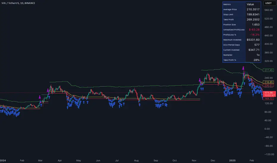
KB Dinamik Grid Bot V8 TrailingThis Pine Script code aims to create a "Dynamic Grid Trading Bot" and perform automatic trading between price ranges. Let's break it down into sections to better understand its functions:
1. Settings and User Inputs
The user can specify the following parameters for the bot:
Lower and Upper Price Limit: Determines the price range where the grid levels are defined.
Number of Grid Lines: Defines how many levels the grid will consist of.
Transaction Amount: Specifies the trading volume for each trading transaction.
Start Date: The date when the bot will start trading.
Price Step (priceStep): Specifies specific steps after the comma to adjust the grid levels more precisely.
Trailing: A feature that activates dynamic selling by following price movements.
2. Calculating Grid Levels
Grid levels: Divides the specified price range into user-defined levels and rounds each level with priceStep.
Lines and labels: Lines and labels are created to visually represent grid levels.
3. Buying and Selling Logic
Buying Transaction: When the price approaches a lower grid level (as much as the offset) and the position is empty, a purchase is made.
Trailing Selling: If Trailing is active, a sale is made when the price passes the specified "trailing step" level.
Normal Selling: If Trailing is not active, a sale is made when the price approaches an upper grid level.
4. Profit and Statistics Tracking
The bot tracks the profit-loss status per transaction and in total.
The number of purchases and sales and net profit information are calculated from the start date.
5. Table Display
The bot places statistical data in a table:
Number of purchases and sales.
Starting date.
Total number of transactions.
Net profit.
Amount of open positions.
6. Drawing and Tracking
Each price movement is updated and the color of the grid lines (green or red) is changed depending on the price's status relative to the level.
This code is a strategy that aims to make a profit by continuously buying and selling in the event of price fluctuations within a range. The "Trailing" feature allows you to keep your profits when the price moves upwards. Net profit, open positions and other statistics are displayed in the table.
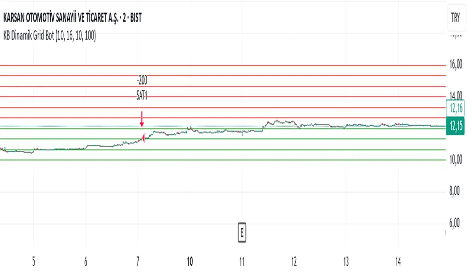
Bullish Reversal Bar Strategy [Skyrexio]Overview
Bullish Reversal Bar Strategy leverages the combination of candlestick pattern Bullish Reversal Bar (description in Methodology and Justification of Methodology), Williams Alligator indicator and Williams Fractals to create the high probability setups. Candlestick pattern is used for the entering into trade, while the combination of Williams Alligator and Fractals is used for the trend approximation as close condition. Strategy uses only long trades.
Unique Features
No fixed stop-loss and take profit: Instead of fixed stop-loss level strategy utilizes technical condition obtained by Fractals and Alligator or the candlestick pattern invalidation to identify when current uptrend is likely to be over (more information in "Methodology" and "Justification of Methodology" paragraphs)
Configurable Trading Periods: Users can tailor the strategy to specific market windows, adapting to different market conditions.
Trend Trade Filter: strategy uses Alligator and Fractal combination as high probability trend filter.
Methodology
The strategy opens long trade when the following price met the conditions:
1.Current candle's high shall be below the Williams Alligator's lines (Jaw, Lips, Teeth)(all details in "Justification of Methodology" paragraph)
2.Price shall create the candlestick pattern "Bullish Reversal Bar". Optionally if MFI and AO filters are enabled current candle shall have the decreasing AO and at least one of three recent bars shall have the squat state on the MFI (all details in "Justification of Methodology" paragraph)
3.If price breaks through the high of the candle marked as the "Bullish Reversal Bar" the long trade is open at the price one tick above the candle's high
4.Initial stop loss is placed at the Bullish Reversal Bar's candle's low
5.If price hit the Bullish Reversal Bar's low before hitting the entry price potential trade is cancelled
6.If trade is active and initial stop loss has not been hit, trade is closed when the combination of Alligator and Williams Fractals shall consider current trend change from upward to downward.
Strategy settings
In the inputs window user can setup strategy setting:
Enable MFI (if true trades are filtered using Market Facilitation Index (MFI) condition all details in "Justification of Methodology" paragraph), by default = false)
Enable AO (if true trades are filtered using Awesome Oscillator (AO) condition all details in "Justification of Methodology" paragraph), by default = false)
Justification of Methodology
Let's explore the key concepts of this strategy and understand how they work together. The first and key concept is the Bullish Reversal Bar candlestick pattern. This is just the single bar pattern. The rules are simple:
Candle shall be closed in it's upper half
High of this candle shall be below all three Alligator's lines (Jaw, Lips, Teeth)
Next, let’s discuss the short-term trend filter, which combines the Williams Alligator and Williams Fractals. Williams Alligator
Developed by Bill Williams, the Alligator is a technical indicator that identifies trends and potential market reversals. It consists of three smoothed moving averages:
Jaw (Blue Line): The slowest of the three, based on a 13-period smoothed moving average shifted 8 bars ahead.
Teeth (Red Line): The medium-speed line, derived from an 8-period smoothed moving average shifted 5 bars forward.
Lips (Green Line): The fastest line, calculated using a 5-period smoothed moving average shifted 3 bars forward.
When the lines diverge and align in order, the "Alligator" is "awake," signaling a strong trend. When the lines overlap or intertwine, the "Alligator" is "asleep," indicating a range-bound or sideways market. This indicator helps traders determine when to enter or avoid trades.
Fractals, another tool by Bill Williams, help identify potential reversal points on a price chart. A fractal forms over at least five consecutive bars, with the middle bar showing either:
Up Fractal: Occurs when the middle bar has a higher high than the two preceding and two following bars, suggesting a potential downward reversal.
Down Fractal: Happens when the middle bar shows a lower low than the surrounding two bars, hinting at a possible upward reversal.
Traders often use fractals alongside other indicators to confirm trends or reversals, enhancing decision-making accuracy.
How do these tools work together in this strategy? Let’s consider an example of an uptrend.
When the price breaks above an up fractal, it signals a potential bullish trend. This occurs because the up fractal represents a shift in market behavior, where a temporary high was formed due to selling pressure. If the price revisits this level and breaks through, it suggests the market sentiment has turned bullish.
The breakout must occur above the Alligator’s teeth line to confirm the trend. A breakout below the teeth is considered invalid, and the downtrend might still persist. Conversely, in a downtrend, the same logic applies with down fractals.
How we can use all these indicators in this strategy? This strategy is a counter trend one. Candle's high shall be below all Alligator's lines. During this market stage the bullish reversal bar candlestick pattern shall be printed. This bar during the downtrend is a high probability setup for the potential reversal to the upside: bulls were able to close the price in the upper half of a candle. The breaking of its high is a high probability signal that trend change is confirmed and script opens long trade. If market continues going down and break down the bullish reversal bar's low potential trend change has been invalidated and strategy close long trade.
If market really reversed and started moving to the upside strategy waits for the trend change form the downtrend to the uptrend according to approximation of Alligator and Fractals combination. If this change happens strategy close the trade. This approach helps to stay in the long trade while the uptrend continuation is likely and close it if there is a high probability of the uptrend finish.
Optionally users can enable MFI and AO filters. First of all, let's briefly explain what are these two indicators. The Awesome Oscillator (AO), created by Bill Williams, is a momentum-based indicator that evaluates market momentum by comparing recent price activity to a broader historical context. It assists traders in identifying potential trend reversals and gauging trend strength.
AO = SMA5(Median Price) − SMA34(Median Price)
where:
Median Price = (High + Low) / 2
SMA5 = 5-period Simple Moving Average of the Median Price
SMA 34 = 34-period Simple Moving Average of the Median Price
This indicator is filtering signals in the following way: if current AO bar is decreasing this candle can be interpreted as a bullish reversal bar. This logic is applicable because initially this strategy is a trend reversal, it is searching for the high probability setup against the current trend. Decreasing AO is the additional high probability filter of a downtrend.
Let's briefly look what is MFI. The Market Facilitation Index (MFI) is a technical indicator that measures the price movement per unit of volume, helping traders gauge the efficiency of price movement in relation to trading volume. Here's how you can calculate it:
MFI = (High−Low)/Volume
MFI can be used in combination with volume, so we can divide 4 states. Bill Williams introduced these to help traders interpret the interaction between volume and price movement. Here’s a quick summary:
Green Window (Increased MFI & Increased Volume): Indicates strong momentum with both price and volume increasing. Often a sign of trend continuation, as both buying and selling interest are rising.
Fake Window (Increased MFI & Decreased Volume): Shows that price is moving but with lower volume, suggesting weak support for the trend. This can signal a potential end of the current trend.
Squat Window (Decreased MFI & Increased Volume): Shows high volume but little price movement, indicating a tug-of-war between buyers and sellers. This often precedes a breakout as the pressure builds.
Fade Window (Decreased MFI & Decreased Volume): Indicates a lack of interest from both buyers and sellers, leading to lower momentum. This typically happens in range-bound markets and may signal consolidation before a new move.
For our purposes we are interested in squat bars. This is the sign that volume cannot move the price easily. This type of bar increases the probability of trend reversal. In this indicator we added to enable the MFI filter of reversal bars. If potential reversal bar or two preceding bars have squat state this bar can be interpret as a reversal one.
Backtest Results
Operating window: Date range of backtests is 2023.01.01 - 2024.12.31. It is chosen to let the strategy to close all opened positions.
Commission and Slippage: Includes a standard Binance commission of 0.1% and accounts for possible slippage over 5 ticks.
Initial capital: 10000 USDT
Percent of capital used in every trade: 50%
Maximum Single Position Loss: -5.29%
Maximum Single Profit: +29.99%
Net Profit: +5472.66 USDT (+54.73%)
Total Trades: 103 (33.98% win rate)
Profit Factor: 1.634
Maximum Accumulated Loss: 1231.15 USDT (-8.32%)
Average Profit per Trade: 53.13 USDT (+0.94%)
Average Trade Duration: 76 hours
How to Use
Add the script to favorites for easy access.
Apply to the desired timeframe and chart (optimal performance observed on 4h ETH/USDT).
Configure settings using the dropdown choice list in the built-in menu.
Set up alerts to automate strategy positions through web hook with the text: {{strategy.order.alert_message}}
Disclaimer:
Educational and informational tool reflecting Skyrex commitment to informed trading. Past performance does not guarantee future results. Test strategies in a simulated environment before live implementation
These results are obtained with realistic parameters representing trading conditions observed at major exchanges such as Binance and with realistic trading portfolio usage parameters.
