YD_Divergence_RSI+CMFThe ‘YD_Divergence_RSI+CMF’ indicator can find divergence using RSI (Relative Strength Index) and CMF (Chaikin Money Flow) indicators.
📌 Key functions
1. Search pivot high and pivot low points in a certain length of price.
2. Connect pivot high to pivot high , pivot low to pivot low , forming two standards for divergence in result.
The marker then plots only the higher high, lower low lines.
(higher low and lower high in prices are referred to hidden divergence, which are not considered in this indicator)
3. Compare the two standards with RSI and CMF indicators, send an alert if there is a divergence. As a result, the indicator will find four combination of divergence.
A. Higher high price / Lower RSI (Bearish RSI Divergence)
B. Lower low price / Higher RSI (Bullish RSI Divergence)
C. Higher high price / Lower CMF (Bearish CMF Divergence)
D. Lower low price / Higher CMF (Bullish CMF Divergence)
📌 Details
Developing the indicators, we put a lot of effort in making a customizable and user-friendly interface.
#1. Pivot Setting
Users can set the length to find the pivot high / pivot low in ‘Pivot Settings – Pivot Length.’
Increased pivot Length takes more candles to interpret the chart but reduce false signals since the it uses only the most certain pivot high / pivot low values. Obviously, decreased pivot length will act the opposite.
Users can choose whether to use ‘High/Low’ or ‘Close’ in ‘Pivot Reference’ to set the swing point of prices.
Users can also choose whether to display the pivot high / pivot low marker on the chart.
#2 RSI & CMF Settings
Users can adjust the length of RSI & CMF separately. (The default values are set to 14 and 20 each.)
#3 Label Setting
Users can adjust the text displayed on the chart label. (The default values is set to ‘Bullish / Bearish’, ‘RSI/CMF’, ‘Divergence’.)
Users can reduce the length of text label or simply turn the label off. Just click the ‘Bull/Bear’ or ‘None’ button. ‘Divergence’ works the same.
Users can decide whether to display the ‘Divergence Line and Label’, set custom settings for the label and line. (color, thickness, style, etc)
📌 Alert
Alert are provided as a combination of the chart's symbol and the set label text. For example,
‘BINANCE:BTCUSDT.P, Bullish RSI Divergence’
====================================================
"YD_Divergence_RSI+CMF" 지표 는 RSI와 CMF 지표를 이용해서 Divergence 를 찾아낼 수 있습니다.
📌 주요 기능
1. 정해진 가격 움직임 안에서 pivot high와 pivot low 포인트 를 찾아냅니다.
2. Pivot high로만 이어진 라인과, Pivot low로만 이어진 두 라인을 작도한 뒤 divergence의 기준으로 삼습니다.
이 지표에서는 normal divergence만 사용하기 때문에 차트에 higher high와 lower low만 표기 합니다.
(higher low와 lower high는 hidden divergence로 정의되며, 이 지표에서는 다루지 않습니다.
3. 두 기준선과 RSI, CMF 지표를 각각 비교하고, 결과적으로 4개의 조합을 구할 수 있습니다.
A. Higher high price / Lower RSI (Bearish RSI Divergence)
B. Lower low price / Higher RSI (Bullish RSI Divergence)
C. Higher high price / Lower CMF (Bearish CMF Divergence)
D. Lower low price / Higher CMF (Bullish CMF Divergence)
📌 세부 사항
지표를 개발하며 사용자들이 원하는 방향으로 지표를 설정할 수 있게 작업에 많은 공을 들였습니다. 굉장히 다양한 옵션을 선택할 수 있으며, 원하는 방식으로 지표를 사용할 수 있습니다.
#1 Pivot Setting
Pivot setting에서는 Pivot Length를 변경할 수 있습니다.
Pivot Length를 늘릴 경우, 보다 확실한 Swing High와 Swing Low만을 사용하게 되므로, False signal이 줄어들 수 있습니다. 하지만 Swing High/ Low를 판정하는 데에 더 긴 시간이 걸리게 되므로, Signal이 다소 늦게 발생하는 단점이 생기게 됩니다.
Pivot Length를 줄일 경우, 반대로 Swing High/Low의 판정이 더 빨리 일어나기 때문에, Signal을 거래에 이용하기는 좋을 수 있습니다. 다만, Swing High와 Low가 훨씬 더 잦은 빈도로 발생하기 때문에 False Signal을 줄 가능성이 높아집니다.
Pivot Reference에서는 가격의 Swing Point를 설정함에 있어, High/Low(고가/저가)를 이용할 지 Close (종가)를 이용할 지 선택할 수 있습니다.
Pivot High/Low Marker를 선택할 경우 Pivot High/ Low에 Marker가 찍히게 됩니다.
#2 RSI와 CMF Setting
RSI와 CMF Setting에서는 RSI와 CMF의 길이를 각각 설정할 수 있습니다. 기본값은 14와 20으로 설정되어 있습니다.
#3 Label Setting
Label Setting에서는 Label에 표시되는 글자를 선택할 수 있습니다.
기본값은 "Bullish / Bearish", "RSI/CMF", "Divergence"로 선택되어 있으며, 너무 길다고 느껴질 경우 "Bull/Bear" 혹은 "None"을 클릭하여 길이를 줄일 수 있습니다. 마찬가지로 Divergence의 경우도 생략이 가능합니다.
하단에서는 Divergence Line과 Label을 켜고 끌 수 있으며, 선의 색깔, 굵기, 종류, 그리고 Label의 색깔, 크기, 종류를 선택할 수 있습니다. Label의 Text 색 역시 변경이 가능합니다.
📌 얼러트
얼러트는 자신이 설정한 차트의 심볼과 Label의 문구의 조합으로 제공되며 예를 들면 다음과 같습니다.
"BINANCE:BTCUSDT.P, Bullish RSI Divergence"
"low" için komut dosyalarını ara

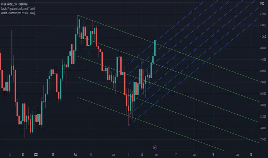
Parallel Projections [theEccentricTrader]█ OVERVIEW
This indicator automatically projects parallel trendlines or channels, from a single point of origin. In the example above I have applied the indicator twice to the 1D SPXUSD. The five upper lines (green) are projected at an angle of -5 from the 1-month swing high anchor point with a projection ratio of -72. And the seven lower lines (blue) are projected at an angle of 10 with a projection ratio of 36 from the 1-week swing low anchor point.
█ CONCEPTS
Green and Red Candles
• A green candle is one that closes with a high price equal to or above the price it opened.
• A red candle is one that closes with a low price that is lower than the price it opened.
Swing Highs and Swing Lows
• A swing high is a green candle or series of consecutive green candles followed by a single red candle to complete the swing and form the peak.
• A swing low is a red candle or series of consecutive red candles followed by a single green candle to complete the swing and form the trough.
Peak and Trough Prices (Basic)
• The peak price of a complete swing high is the high price of either the red candle that completes the swing high or the high price of the preceding green candle, depending on which is higher.
• The trough price of a complete swing low is the low price of either the green candle that completes the swing low or the low price of the preceding red candle, depending on which is lower.
Historic Peaks and Troughs
The current, or most recent, peak and trough occurrences are referred to as occurrence zero. Previous peak and trough occurrences are referred to as historic and ordered numerically from right to left, with the most recent historic peak and trough occurrences being occurrence one.
Support and Resistance
• Support refers to a price level where the demand for an asset is strong enough to prevent the price from falling further.
• Resistance refers to a price level where the supply of an asset is strong enough to prevent the price from rising further.
Support and resistance levels are important because they can help traders identify where the price of an asset might pause or reverse its direction, offering potential entry and exit points. For example, a trader might look to buy an asset when it approaches a support level , with the expectation that the price will bounce back up. Alternatively, a trader might look to sell an asset when it approaches a resistance level , with the expectation that the price will drop back down.
It's important to note that support and resistance levels are not always relevant, and the price of an asset can also break through these levels and continue moving in the same direction.
Trendlines
Trendlines are straight lines that are drawn between two or more points on a price chart. These lines are used as dynamic support and resistance levels for making strategic decisions and predictions about future price movements. For example traders will look for price movements along, and reactions to, trendlines in the form of rejections or breakouts/downs.
█ FEATURES
Inputs
• Anchor Point Type
• Swing High/Low Occurrence
• HTF Resolution
• Highest High/Lowest Low Lookback
• Angle Degree
• Projection Ratio
• Number Lines
• Line Color
Anchor Point Types
• Swing High
• Swing Low
• Swing High (HTF)
• Swing Low (HTF)
• Highest High
• Lowest Low
• Intraday Highest High (intraday charts only)
• Intraday Lowest Low (intraday charts only)
Swing High/Swing Low Occurrence
This input is used to determine which historic peak or trough to reference for swing high or swing low anchor point types.
HTF Resolution
This input is used to determine which higher timeframe to reference for swing high (HTF) or swing low (HTF) anchor point types.
Highest High/Lowest Low Lookback
This input is used to determine the lookback length for highest high or lowest low anchor point types.
Intraday Highest High/Lowest Low Lookback
When using intraday highest high or lowest low anchor point types, the lookback length is calculated automatically based on number of bars since the daily candle opened.
Angle Degree
This input is used to determine the angle of the trendlines. The output is expressed in terms of point or pips, depending on the symbol type, which is then passed through the built in math.todegrees() function. Positive numbers will project the lines upwards while negative numbers will project the lines downwards. Depending on the market and timeframe, the impact input values will have on the visible gaps between the lines will vary greatly. For example, an input of 10 will have a far greater impact on the gaps between the lines when viewed from the 1-minute timeframe than it would on the 1-day timeframe. The input is a float and as such the value passed through can go into as many decimal places as the user requires.
It is also worth mentioning that as more lines are added the gaps between the lines, that are closest to the anchor point, will get tighter as they make their way up the y-axis. Although the gaps between the lines will stay constant at the x2 plot, i.e. a distance of 10 points between them, they will gradually get tighter and tighter at the point of origin as the slope of the lines get steeper.
Projection Ratio
This input is used to determine the distance between the parallels, expressed in terms of point or pips. Positive numbers will project the lines upwards while negative numbers will project the lines downwards. Depending on the market and timeframe, the impact input values will have on the visible gaps between the lines will vary greatly. For example, an input of 10 will have a far greater impact on the gaps between the lines when viewed from the 1-minute timeframe than it would on the 1-day timeframe. The input is a float and as such the value passed through can go into as many decimal places as the user requires.
Number Lines
This input is used to determine the number of lines to be drawn on the chart, maximum is 500.
█ LIMITATIONS
All green and red candle calculations are based on differences between open and close prices, as such I have made no attempt to account for green candles that gap lower and close below the close price of the preceding candle, or red candles that gap higher and close above the close price of the preceding candle. This may cause some unexpected behaviour on some markets and timeframes. I can only recommend using 24-hour markets, if and where possible, as there are far fewer gaps and, generally, more data to work with.
If the lines do not draw or you see a study error saying that the script references too many candles in history, this is most likely because the higher timeframe anchor point is not present on the current timeframe. This problem usually occurs when referencing a higher timeframe, such as the 1-month, from a much lower timeframe, such as the 1-minute. How far you can lookback for higher timeframe anchor points on the current timeframe will also be limited by your Trading View subscription plan. Premium users get 20,000 candles worth of data, pro+ and pro users get 10,000, and basic users get 5,000.
█ RAMBLINGS
It is my current thesis that the indicator will work best when used in conjunction with my Wavemeter indicator, which can be used to set the angle and projection ratio. For example, the average wave height or amplitude could be used as the value for the angle and projection ratio inputs. Or some factor or multiple of such an average. I think this makes sense as it allows for objectivity when applying the indicator across different markets and timeframes with different energies and vibrations.
“If you want to find the secrets of the universe, think in terms of energy, frequency and vibration.”
― Nikola Tesla
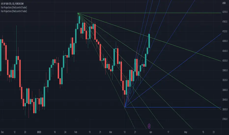
Fan Projections [theEccentricTrader]█ OVERVIEW
This indicator automatically projects trendlines in the shape of a fan, from a single point of origin. In the example above I have applied the indicator twice to the 1D SPXUSD. The seven upper lines (green) are projected at an angle of -5 from the 1-month swing high anchor point. And the five lower lines (blue) are projected at an angle of 10 from the 1-week swing low anchor point.
█ CONCEPTS
Green and Red Candles
• A green candle is one that closes with a high price equal to or above the price it opened.
• A red candle is one that closes with a low price that is lower than the price it opened.
Swing Highs and Swing Lows
• A swing high is a green candle or series of consecutive green candles followed by a single red candle to complete the swing and form the peak.
• A swing low is a red candle or series of consecutive red candles followed by a single green candle to complete the swing and form the trough.
Peak and Trough Prices (Basic)
• The peak price of a complete swing high is the high price of either the red candle that completes the swing high or the high price of the preceding green candle, depending on which is higher.
• The trough price of a complete swing low is the low price of either the green candle that completes the swing low or the low price of the preceding red candle, depending on which is lower.
Historic Peaks and Troughs
The current, or most recent, peak and trough occurrences are referred to as occurrence zero. Previous peak and trough occurrences are referred to as historic and ordered numerically from right to left, with the most recent historic peak and trough occurrences being occurrence one.
Support and Resistance
• Support refers to a price level where the demand for an asset is strong enough to prevent the price from falling further.
• Resistance refers to a price level where the supply of an asset is strong enough to prevent the price from rising further.
Support and resistance levels are important because they can help traders identify where the price of an asset might pause or reverse its direction, offering potential entry and exit points. For example, a trader might look to buy an asset when it approaches a support level , with the expectation that the price will bounce back up. Alternatively, a trader might look to sell an asset when it approaches a resistance level , with the expectation that the price will drop back down.
It's important to note that support and resistance levels are not always relevant, and the price of an asset can also break through these levels and continue moving in the same direction.
Trendlines
Trendlines are straight lines that are drawn between two or more points on a price chart. These lines are used as dynamic support and resistance levels for making strategic decisions and predictions about future price movements. For example traders will look for price movements along, and reactions to, trendlines in the form of rejections or breakouts/downs.
█ FEATURES
Inputs
• Anchor Point Type
• Swing High/Low Occurrence
• HTF Resolution
• Highest High/Lowest Low Lookback
• Angle Degree
• Number Lines
• Line Color
Anchor Point Types
• Swing High
• Swing Low
• Swing High (HTF)
• Swing Low (HTF)
• Highest High
• Lowest Low
• Intraday Highest High (intraday charts only)
• Intraday Lowest Low (intraday charts only)
Swing High/Swing Low Occurrence
This input is used to determine which historic peak or trough to reference for swing high or swing low anchor point types.
HTF Resolution
This input is used to determine which higher timeframe to reference for swing high (HTF) or swing low (HTF) anchor point types.
Highest High/Lowest Low Lookback
This input is used to determine the lookback length for highest high or lowest low anchor point types.
Intraday Highest High/Lowest Low Lookback
When using intraday highest high or lowest low anchor point types, the lookback length is calculated automatically based on number of bars since the daily candle opened.
Angle Degree
This input is used to determine the angle of the trendlines. The output is expressed in terms of point or pips, depending on the symbol type, which is then passed through the built in math.todegrees() function. Positive numbers will project the lines upwards while negative numbers will project the lines downwards. Depending on the market and timeframe, the impact input values will have on the visible gaps between the lines will vary greatly. For example, an input of 10 will have a far greater impact on the gaps between the lines when viewed from the 1-minute timeframe than it would on the 1-day timeframe. The input is a float and as such the value passed through can go into as many decimal places as the user requires.
It is also worth mentioning that as more lines are added the gaps between the lines, that are closest to the anchor point, will get tighter as they make their way up the y-axis. Although the gaps between the lines will stay constant at the x2 plot, i.e. a distance of 10 points between them, they will gradually get tighter and tighter at the point of origin as the slope of the lines get steeper.
Number Lines
This input is used to determine the number of lines to be drawn on the chart, maximum is 500.
█ LIMITATIONS
All green and red candle calculations are based on differences between open and close prices, as such I have made no attempt to account for green candles that gap lower and close below the close price of the preceding candle, or red candles that gap higher and close above the close price of the preceding candle. This may cause some unexpected behaviour on some markets and timeframes. I can only recommend using 24-hour markets, if and where possible, as there are far fewer gaps and, generally, more data to work with.
If the lines do not draw or you see a study error saying that the script references too many candles in history, this is most likely because the higher timeframe anchor point is not present on the current timeframe. This problem usually occurs when referencing a higher timeframe, such as the 1-month, from a much lower timeframe, such as the 1-minute. How far you can lookback for higher timeframe anchor points on the current timeframe will also be limited by your Trading View subscription plan. Premium users get 20,000 candles worth of data, pro+ and pro users get 10,000, and basic users get 5,000.
█ RAMBLINGS
It is my current thesis that the indicator will work best when used in conjunction with my Wavemeter indicator, which can be used to set the angle. For example, the average wave height or amplitude could be used as the value for the angle input. Or some factor or multiple of such an average. I think this makes sense as it allows for objectivity when applying the indicator across different markets and timeframes with different energies and vibrations.
“If you want to find the secrets of the universe, think in terms of energy, frequency and vibration.”
― Nikola Tesla
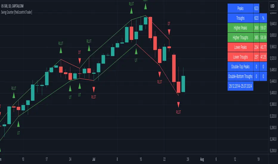
Swing Counter [theEccentricTrader]█ OVERVIEW
This indicator counts the number of confirmed swing high and swing low scenarios on any given candlestick chart and displays the statistics in a table, which can be repositioned and resized at the user's discretion.
█ CONCEPTS
Green and Red Candles
• A green candle is one that closes with a high price equal to or above the price it opened.
• A red candle is one that closes with a low price that is lower than the price it opened.
Swing Highs and Swing Lows
• A swing high is a green candle or series of consecutive green candles followed by a single red candle to complete the swing and form the peak.
• A swing low is a red candle or series of consecutive red candles followed by a single green candle to complete the swing and form the trough.
Peak and Trough Prices (Basic)
• The peak price of a complete swing high is the high price of either the red candle that completes the swing high or the high price of the preceding green candle, depending on which is higher.
• The trough price of a complete swing low is the low price of either the green candle that completes the swing low or the low price of the preceding red candle, depending on which is lower.
Peak and Trough Prices (Advanced)
• The advanced peak price of a complete swing high is the high price of either the red candle that completes the swing high or the high price of the highest preceding green candle high price, depending on which is higher.
• The advanced trough price of a complete swing low is the low price of either the green candle that completes the swing low or the low price of the lowest preceding red candle low price, depending on which is lower.
Green and Red Peaks and Troughs
• A green peak is one that derives its price from the green candle/s that constitute the swing high.
• A red peak is one that derives its price from the red candle that completes the swing high.
• A green trough is one that derives its price from the green candle that completes the swing low.
• A red trough is one that derives its price from the red candle/s that constitute the swing low.
Historic Peaks and Troughs
The current, or most recent, peak and trough occurrences are referred to as occurrence zero. Previous peak and trough occurrences are referred to as historic and ordered numerically from right to left, with the most recent historic peak and trough occurrences being occurrence one.
Upper Trends
• A return line uptrend is formed when the current peak price is higher than the preceding peak price.
• A downtrend is formed when the current peak price is lower than the preceding peak price.
• A double-top is formed when the current peak price is equal to the preceding peak price.
Lower Trends
• An uptrend is formed when the current trough price is higher than the preceding trough price.
• A return line downtrend is formed when the current trough price is lower than the preceding trough price.
• A double-bottom is formed when the current trough price is equal to the preceding trough price.
█ FEATURES
Inputs
• Start Date
• End Date
• Position
• Text Size
• Show Sample Period
• Show Plots
• Show Lines
Table
The table is colour coded, consists of three columns and nine rows. Blue cells denote neutral scenarios, green cells denote return line uptrend and uptrend scenarios, and red cells denote downtrend and return line downtrend scenarios.
The swing scenarios are listed in the first column with their corresponding total counts to the right, in the second column. The last row in column one, row nine, displays the sample period which can be adjusted or hidden via indicator settings.
Rows three and four in the third column of the table display the total higher peaks and higher troughs as percentages of total peaks and troughs, respectively. Rows five and six in the third column display the total lower peaks and lower troughs as percentages of total peaks and troughs, respectively. And rows seven and eight display the total double-top peaks and double-bottom troughs as percentages of total peaks and troughs, respectively.
Plots
I have added plots as a visual aid to the swing scenarios listed in the table. Green up-arrows with ‘HP’ denote higher peaks, while green up-arrows with ‘HT’ denote higher troughs. Red down-arrows with ‘LP’ denote higher peaks, while red down-arrows with ‘LT’ denote lower troughs. Similarly, blue diamonds with ‘DT’ denote double-top peaks and blue diamonds with ‘DB’ denote double-bottom troughs. These plots can be hidden via indicator settings.
Lines
I have also added green and red trendlines as a further visual aid to the swing scenarios listed in the table. Green lines denote return line uptrends (higher peaks) and uptrends (higher troughs), while red lines denote downtrends (lower peaks) and return line downtrends (lower troughs). These lines can be hidden via indicator settings.
█ HOW TO USE
This indicator is intended for research purposes and strategy development. I hope it will be useful in helping to gain a better understanding of the underlying dynamics at play on any given market and timeframe. It can, for example, give you an idea of any inherent biases such as a greater proportion of higher peaks to lower peaks. Or a greater proportion of higher troughs to lower troughs. Such information can be very useful when conducting top down analysis across multiple timeframes, or considering entry and exit methods.
What I find most fascinating about this logic, is that the number of swing highs and swing lows will always find equilibrium on each new complete wave cycle. If for example the chart begins with a swing high and ends with a swing low there will be an equal number of swing highs to swing lows. If the chart starts with a swing high and ends with a swing high there will be a difference of one between the two total values until another swing low is formed to complete the wave cycle sequence that began at start of the chart. Almost as if it was a fundamental truth of price action, although quite common sensical in many respects. As they say, what goes up must come down.
The objective logic for swing highs and swing lows I hope will form somewhat of a foundational building block for traders, researchers and developers alike. Not only does it facilitate the objective study of swing highs and swing lows it also facilitates that of ranges, trends, double trends, multi-part trends and patterns. The logic can also be used for objective anchor points. Concepts I will introduce and develop further in future publications.
█ LIMITATIONS
Some higher timeframe candles on tickers with larger lookbacks such as the DXY , do not actually contain all the open, high, low and close (OHLC) data at the beginning of the chart. Instead, they use the close price for open, high and low prices. So, while we can determine whether the close price is higher or lower than the preceding close price, there is no way of knowing what actually happened intra-bar for these candles. And by default candles that close at the same price as the open price, will be counted as green. You can avoid this problem by utilising the sample period filter.
The green and red candle calculations are based solely on differences between open and close prices, as such I have made no attempt to account for green candles that gap lower and close below the close price of the preceding candle, or red candles that gap higher and close above the close price of the preceding candle. I can only recommend using 24-hour markets, if and where possible, as there are far fewer gaps and, generally, more data to work with. Alternatively, you can replace the scenarios with your own logic to account for the gap anomalies, if you are feeling up to the challenge.
The sample size will be limited to your Trading View subscription plan. Premium users get 20,000 candles worth of data, pro+ and pro users get 10,000, and basic users get 5,000. If upgrading is currently not an option, you can always keep a rolling tally of the statistics in an excel spreadsheet or something of the like.
█ NOTES
I feel it important to address the mention of advanced peak and trough price logic. While I have introduced the concept, I have not included the logic in my script for a number of reasons. The most pertinent of which being the amount of extra work I would have to do to include it in a public release versus the actual difference it would make to the statistics. Based on my experience, there are actually only a small number of cases where the advanced peak and trough prices are different from the basic peak and trough prices. And with adequate multi-timeframe analysis any high or low prices that are not captured using basic peak and trough price logic on any given time frame, will no doubt be captured on a higher timeframe. See the example below on the 1H FOREXCOM:USDJPY chart (Figure 1), where the basic peak price logic denoted by the indicator plot does not capture what would be the advanced peak price, but on the 2H FOREXCOM:USDJPY chart (Figure 2), the basic peak logic does capture the advanced peak price from the 1H timeframe.
Figure 1.
Figure 2.
█ RAMBLINGS
“Never was there an age that placed economic interests higher than does our own. Never was the need of a scientific foundation for economic affairs felt more generally or more acutely. And never was the ability of practical men to utilize the achievements of science, in all fields of human activity, greater than in our day. If practical men, therefore, rely wholly on their own experience, and disregard our science in its present state of development, it cannot be due to a lack of serious interest or ability on their part. Nor can their disregard be the result of a haughty rejection of the deeper insight a true science would give into the circumstances and relationships determining the outcome of their activity. The cause of such remarkable indifference must not be sought elsewhere than in the present state of our science itself, in the sterility of all past endeavours to find its empirical foundations.” (Menger, 1871, p.45).
█ BIBLIOGRAPHY
Menger, C. (1871) Principles of Economics. Reprint, Auburn, Alabama: Ludwig Von Mises Institute: 2007.
Failed Breakdown Detection'Failed Breakdowns' are a popular set up for long entries.
In short, the set up requires:
1) A significant low is made ('initial low')
2) Initial low is undercut with a new low
3) Price action then 'reclaims' the initial low by moving +8-10 points from the initial low
This script aims at detecting such set ups. It was coded with the ES Futures 15 minute chart in mind but may be useful on other instruments and time frames.
Business Logic:
1) Uses pivot lows to detect 'significant' initial lows
2) Uses amplitude threshold to detect a new low beneath the initial low; used /u/ben_zen script for this
3) Looks for a valid reclaim - a green candle that occurs within 10 bars of the new low
4) Price must reclaim at least 8 points for the set up to be valid
5) If a signal is detected, the initial low value (pivot low) is stored in array that prevents duplicate signals from being generated.
6) FBD Signal is plotted on the chart with "X"
7) Pivot low detection is plotted on the chart with "P" and a label
8) New lows are plotted on the chart with a blue triangle
Notes:
User input
- My preference is to use the defaults as is, but as always feel free to experiment
- Can modify pivot length but in my experience 10/10 work best for pivot lows
- New low detection - 55 bars and 0.05 amplitude work well based on visual checks of signals
- Can modify the number of points needed to reclaim a low, and the # of bars limit under which this must occur.
Alerts:
- Alerts are available for detection of new lows and detection of failed breakdowns
- Alerts are also available for these signals but only during 7:30PM-4PM EST - 'prime time' US trading hours
Limitations:
- Current version of the script only compares new lows to the most recent pivot low, does not look at anything prior to that
- Best used as a discretionary signal
Visit /u/ben_zen's Profile:
www.tradingview.com
Profile Link www.tradingview.com

Larry Williams Strategies IndicatorThis indicator is a trend following indicator. It plots some of the trend following strategies described by Larry Williams in his book 'Long Term Secrets to Short Term Trading'. Below are types of trend following strategies you can trade using this indicator. These are notes taken directly from Larry Williams' book.
Short Term Low Strategy
Short Term Low - Any daily low with higher lows on each side of it.
Intermediate Term Low – Any short term low with higher short term lows on each side of it.
Long Term Low – Any intermediate term low with higher intermediate term lows on each side of it.
Conceptual pattern for best buying opportunity is when forming an intermediate term low higher than the last intermediate term low.
This setup can be used on all time frames. However since Larry Williams usually trades the daily chart, the daily chart is probably the best timeframe to trade using this strategy.
Entry point – High of the day that has a higher high on the right side of it.
(My interpretation: price crossing above the high of the previous day is the buy signal)
Target – Markets have a strong tendency to rally above the last intermediate term high by the same amount it moved from the last intermediate term high to the lowest point prior to advancing to new highs.
Trailing Stop – Set stop to most recent short term low, move up as new short term lows are formed. Can also use formation of next intermediate term high as an exit point.
A 'run' to the upside is over when price fails to move higher the next day and falls below the prior day's low.
Short Term High Strategy
Short Term High - Any daily high with lower highs on each side of it.
Intermediate Term High – Any short term high with lower short term highs on each side of it.
Long Term High – Any intermediate term high with lower intermediate term highs on each side of it.
Conceptual pattern for best selling opportunity is when forming an intermediate term high lower than the last intermediate term high.
This setup can be used on all time frames. However since Larry Williams usually trades the daily chart, the daily chart is probably the best timeframe to trade using this strategy.
Entry point – Low of the day that has a lower low on the right side of it.
(My interpretation: price crossing below the low of the previous day is the sell short signal)
Target – Markets have a strong tendency to fall below the last intermediate term low by the same amount it moved from the last intermediate term low to the highest point prior to declining to new lows.
Trailing Stop – Set stop to most recent short term high, move down as new short term highs are formed. Can also use formation of next intermediate term low as an exit point.
A 'run' to the downside is over when price fails to move lower the next day and rises above the prior day's high.
Trend Reversals
A trend change from down to up occurs when a short term high is exceeded on the upside, a trend change from up to down is identified by price going below the most recent low.
Can take these signals to make trades, but it is best to filter them with a confirmation or edge such as Trading Day of the Week, Trading Day of the Month, trendlines, etc. to cut down on false signals.
Three Bar High/Low System
Calculate a three bar moving average of the highs and a three bar moving average of the lows.
Strategy is to buy at the at the price of the three bar moving average of the lows - if the trend is positive according to the swing point trend identification technique - and take profits at the three bar moving average of the highs.
Selling is just the opposite. Sell short at the three bar moving average of the highs and take profits at the three bar moving average of the lows, using the trend identification technique above for confirmation.
This strategy can work on any timeframe, but was described as a daytrading system by Larry Williams.

Kripto Fema ind/ This Pine Script™ code is subject to the terms of the Mozilla Public License 2.0 at mozilla.org
// © Femayakup
//@version=5
indicator(title = "Kripto Fema ind", shorttitle="Kripto Fema ind", overlay=true, format=format.price, precision=2,max_lines_count = 500, max_labels_count = 500, max_bars_back=500)
showEma200 = input(true, title="EMA 200")
showPmax = input(true, title="Pmax")
showLinreg = input(true, title="Linreg")
showMavilim = input(true, title="Mavilim")
showNadaray = input(true, title="Nadaraya Watson")
ma(source, length, type) =>
switch type
"SMA" => ta.sma(source, length)
"EMA" => ta.ema(source, length)
"SMMA (RMA)" => ta.rma(source, length)
"WMA" => ta.wma(source, length)
"VWMA" => ta.vwma(source, length)
//Ema200
timeFrame = input.timeframe(defval = '240',title= 'EMA200 TimeFrame',group = 'EMA200 Settings')
len200 = input.int(200, minval=1, title="Length",group = 'EMA200 Settings')
src200 = input(close, title="Source",group = 'EMA200 Settings')
offset200 = input.int(title="Offset", defval=0, minval=-500, maxval=500,group = 'EMA200 Settings')
out200 = ta.ema(src200, len200)
higherTimeFrame = request.security(syminfo.tickerid,timeFrame,out200 ,barmerge.gaps_on,barmerge.lookahead_on)
ema200Plot = showEma200 ? higherTimeFrame : na
plot(ema200Plot, title="EMA200", offset=offset200)
//Linreq
group1 = "Linreg Settings"
lengthInput = input.int(100, title="Length", minval = 1, maxval = 5000,group = group1)
sourceInput = input.source(close, title="Source")
useUpperDevInput = input.bool(true, title="Upper Deviation", inline = "Upper Deviation", group = group1)
upperMultInput = input.float(2.0, title="", inline = "Upper Deviation", group = group1)
useLowerDevInput = input.bool(true, title="Lower Deviation", inline = "Lower Deviation", group = group1)
lowerMultInput = input.float(2.0, title="", inline = "Lower Deviation", group = group1)
group2 = "Linreg Display Settings"
showPearsonInput = input.bool(true, "Show Pearson's R", group = group2)
extendLeftInput = input.bool(false, "Extend Lines Left", group = group2)
extendRightInput = input.bool(true, "Extend Lines Right", group = group2)
extendStyle = switch
extendLeftInput and extendRightInput => extend.both
extendLeftInput => extend.left
extendRightInput => extend.right
=> extend.none
group3 = "Linreg Color Settings"
colorUpper = input.color(color.new(color.blue, 85), "Linreg Renk", inline = group3, group = group3)
colorLower = input.color(color.new(color.red, 85), "", inline = group3, group = group3)
calcSlope(source, length) =>
max_bars_back(source, 5000)
if not barstate.islast or length <= 1
else
sumX = 0.0
sumY = 0.0
sumXSqr = 0.0
sumXY = 0.0
for i = 0 to length - 1 by 1
val = source
per = i + 1.0
sumX += per
sumY += val
sumXSqr += per * per
sumXY += val * per
slope = (length * sumXY - sumX * sumY) / (length * sumXSqr - sumX * sumX)
average = sumY / length
intercept = average - slope * sumX / length + slope
= calcSlope(sourceInput, lengthInput)
startPrice = i + s * (lengthInput - 1)
endPrice = i
var line baseLine = na
if na(baseLine) and not na(startPrice) and showLinreg
baseLine := line.new(bar_index - lengthInput + 1, startPrice, bar_index, endPrice, width=1, extend=extendStyle, color=color.new(colorLower, 0))
else
line.set_xy1(baseLine, bar_index - lengthInput + 1, startPrice)
line.set_xy2(baseLine, bar_index, endPrice)
na
calcDev(source, length, slope, average, intercept) =>
upDev = 0.0
dnDev = 0.0
stdDevAcc = 0.0
dsxx = 0.0
dsyy = 0.0
dsxy = 0.0
periods = length - 1
daY = intercept + slope * periods / 2
val = intercept
for j = 0 to periods by 1
price = high - val
if price > upDev
upDev := price
price := val - low
if price > dnDev
dnDev := price
price := source
dxt = price - average
dyt = val - daY
price -= val
stdDevAcc += price * price
dsxx += dxt * dxt
dsyy += dyt * dyt
dsxy += dxt * dyt
val += slope
stdDev = math.sqrt(stdDevAcc / (periods == 0 ? 1 : periods))
pearsonR = dsxx == 0 or dsyy == 0 ? 0 : dsxy / math.sqrt(dsxx * dsyy)
= calcDev(sourceInput, lengthInput, s, a, i)
upperStartPrice = startPrice + (useUpperDevInput ? upperMultInput * stdDev : upDev)
upperEndPrice = endPrice + (useUpperDevInput ? upperMultInput * stdDev : upDev)
var line upper = na
lowerStartPrice = startPrice + (useLowerDevInput ? -lowerMultInput * stdDev : -dnDev)
lowerEndPrice = endPrice + (useLowerDevInput ? -lowerMultInput * stdDev : -dnDev)
var line lower = na
if na(upper) and not na(upperStartPrice) and showLinreg
upper := line.new(bar_index - lengthInput + 1, upperStartPrice, bar_index, upperEndPrice, width=1, extend=extendStyle, color=color.new(colorUpper, 0))
else
line.set_xy1(upper, bar_index - lengthInput + 1, upperStartPrice)
line.set_xy2(upper, bar_index, upperEndPrice)
na
if na(lower) and not na(lowerStartPrice) and showLinreg
lower := line.new(bar_index - lengthInput + 1, lowerStartPrice, bar_index, lowerEndPrice, width=1, extend=extendStyle, color=color.new(colorUpper, 0))
else
line.set_xy1(lower, bar_index - lengthInput + 1, lowerStartPrice)
line.set_xy2(lower, bar_index, lowerEndPrice)
na
showLinregPlotUpper = showLinreg ? upper : na
showLinregPlotLower = showLinreg ? lower : na
showLinregPlotBaseLine = showLinreg ? baseLine : na
linefill.new(showLinregPlotUpper, showLinregPlotBaseLine, color = colorUpper)
linefill.new(showLinregPlotBaseLine, showLinregPlotLower, color = colorLower)
// Pearson's R
var label r = na
label.delete(r )
if showPearsonInput and not na(pearsonR) and showLinreg
r := label.new(bar_index - lengthInput + 1, lowerStartPrice, str.tostring(pearsonR, "#.################"), color = color.new(color.white, 100), textcolor=color.new(colorUpper, 0), size=size.normal, style=label.style_label_up)
//Mavilim
group4 = "Mavilim Settings"
mavilimold = input(false, title="Show Previous Version of MavilimW?",group=group4)
fmal=input(3,"First Moving Average length",group = group4)
smal=input(5,"Second Moving Average length",group = group4)
tmal=fmal+smal
Fmal=smal+tmal
Ftmal=tmal+Fmal
Smal=Fmal+Ftmal
M1= ta.wma(close, fmal)
M2= ta.wma(M1, smal)
M3= ta.wma(M2, tmal)
M4= ta.wma(M3, Fmal)
M5= ta.wma(M4, Ftmal)
MAVW= ta.wma(M5, Smal)
col1= MAVW>MAVW
col3= MAVWpmaxsrc ? pmaxsrc-pmaxsrc : 0
vdd1=pmaxsrc
ma = 0.0
if mav == "SMA"
ma := ta.sma(pmaxsrc, length)
ma
if mav == "EMA"
ma := ta.ema(pmaxsrc, length)
ma
if mav == "WMA"
ma := ta.wma(pmaxsrc, length)
ma
if mav == "TMA"
ma := ta.sma(ta.sma(pmaxsrc, math.ceil(length / 2)), math.floor(length / 2) + 1)
ma
if mav == "VAR"
ma := VAR
ma
if mav == "WWMA"
ma := WWMA
ma
if mav == "ZLEMA"
ma := ZLEMA
ma
if mav == "TSF"
ma := TSF
ma
ma
MAvg=getMA(pmaxsrc, length)
longStop = Normalize ? MAvg - Multiplier*atr/close : MAvg - Multiplier*atr
longStopPrev = nz(longStop , longStop)
longStop := MAvg > longStopPrev ? math.max(longStop, longStopPrev) : longStop
shortStop = Normalize ? MAvg + Multiplier*atr/close : MAvg + Multiplier*atr
shortStopPrev = nz(shortStop , shortStop)
shortStop := MAvg < shortStopPrev ? math.min(shortStop, shortStopPrev) : shortStop
dir = 1
dir := nz(dir , dir)
dir := dir == -1 and MAvg > shortStopPrev ? 1 : dir == 1 and MAvg < longStopPrev ? -1 : dir
PMax = dir==1 ? longStop: shortStop
plot(showsupport ? MAvg : na, color=#fbff04, linewidth=2, title="EMA9")
pALL=plot(PMax, color=color.new(color.red, transp = 0), linewidth=2, title="PMax")
alertcondition(ta.cross(MAvg, PMax), title="Cross Alert", message="PMax - Moving Avg Crossing!")
alertcondition(ta.crossover(MAvg, PMax), title="Crossover Alarm", message="Moving Avg BUY SIGNAL!")
alertcondition(ta.crossunder(MAvg, PMax), title="Crossunder Alarm", message="Moving Avg SELL SIGNAL!")
alertcondition(ta.cross(pmaxsrc, PMax), title="Price Cross Alert", message="PMax - Price Crossing!")
alertcondition(ta.crossover(pmaxsrc, PMax), title="Price Crossover Alarm", message="PRICE OVER PMax - BUY SIGNAL!")
alertcondition(ta.crossunder(pmaxsrc, PMax), title="Price Crossunder Alarm", message="PRICE UNDER PMax - SELL SIGNAL!")
buySignalk = ta.crossover(MAvg, PMax)
plotshape(buySignalk and showsignalsk ? PMax*0.995 : na, title="Buy", text="Buy", location=location.absolute, style=shape.labelup, size=size.tiny, color=color.new(color.green, transp = 0), textcolor=color.white)
sellSignallk = ta.crossunder(MAvg, PMax)
plotshape(sellSignallk and showsignalsk ? PMax*1.005 : na, title="Sell", text="Sell", location=location.absolute, style=shape.labeldown, size=size.tiny, color=color.new(color.red, transp = 0), textcolor=color.white)
// buySignalc = ta.crossover(pmaxsrc, PMax)
// plotshape(buySignalc and showsignalsc ? PMax*0.995 : na, title="Buy", text="Buy", location=location.absolute, style=shape.labelup, size=size.tiny, color=#0F18BF, textcolor=color.white)
// sellSignallc = ta.crossunder(pmaxsrc, PMax)
// plotshape(sellSignallc and showsignalsc ? PMax*1.005 : na, title="Sell", text="Sell", location=location.absolute, style=shape.labeldown, size=size.tiny, color=#0F18BF, textcolor=color.white)
// mPlot = plot(ohlc4, title="", style=plot.style_circles, linewidth=0,display=display.none)
longFillColor = highlighting ? (MAvg>PMax ? color.new(color.green, transp = 90) : na) : na
shortFillColor = highlighting ? (MAvg math.exp(-(math.pow(x, 2)/(h * h * 2)))
//-----------------------------------------------------------------------------}
//Append lines
//-----------------------------------------------------------------------------{
n = bar_index
var ln = array.new_line(0)
if barstate.isfirst and repaint
for i = 0 to 499
array.push(ln,line.new(na,na,na,na))
//-----------------------------------------------------------------------------}
//End point method
//-----------------------------------------------------------------------------{
var coefs = array.new_float(0)
var den = 0.
if barstate.isfirst and not repaint
for i = 0 to 499
w = gauss(i, h)
coefs.push(w)
den := coefs.sum()
out = 0.
if not repaint
for i = 0 to 499
out += src * coefs.get(i)
out /= den
mae = ta.sma(math.abs(src - out), 499) * mult
upperN = out + mae
lowerN = out - mae
//-----------------------------------------------------------------------------}
//Compute and display NWE
//-----------------------------------------------------------------------------{
float y2 = na
float y1 = na
nwe = array.new(0)
if barstate.islast and repaint
sae = 0.
//Compute and set NWE point
for i = 0 to math.min(499,n - 1)
sum = 0.
sumw = 0.
//Compute weighted mean
for j = 0 to math.min(499,n - 1)
w = gauss(i - j, h)
sum += src * w
sumw += w
y2 := sum / sumw
sae += math.abs(src - y2)
nwe.push(y2)
sae := sae / math.min(499,n - 1) * mult
for i = 0 to math.min(499,n - 1)
if i%2 and showNadaray
line.new(n-i+1, y1 + sae, n-i, nwe.get(i) + sae, color = upCss)
line.new(n-i+1, y1 - sae, n-i, nwe.get(i) - sae, color = dnCss)
if src > nwe.get(i) + sae and src < nwe.get(i) + sae and showNadaray
label.new(n-i, src , '▼', color = color(na), style = label.style_label_down, textcolor = dnCss, textalign = text.align_center)
if src < nwe.get(i) - sae and src > nwe.get(i) - sae and showNadaray
label.new(n-i, src , '▲', color = color(na), style = label.style_label_up, textcolor = upCss, textalign = text.align_center)
y1 := nwe.get(i)
//-----------------------------------------------------------------------------}
//Dashboard
//-----------------------------------------------------------------------------{
var tb = table.new(position.top_right, 1, 1
, bgcolor = #1e222d
, border_color = #373a46
, border_width = 1
, frame_color = #373a46
, frame_width = 1)
if repaint
tb.cell(0, 0, 'Repainting Mode Enabled', text_color = color.white, text_size = size.small)
//-----------------------------------------------------------------------------}
//Plot
//-----------------------------------------------------------------------------}
// plot(repaint ? na : out + mae, 'Upper', upCss)
// plot(repaint ? na : out - mae, 'Lower', dnCss)
//Crossing Arrows
// plotshape(ta.crossunder(close, out - mae) ? low : na, "Crossunder", shape.labelup, location.absolute, color(na), 0 , text = '▲', textcolor = upCss, size = size.tiny)
// plotshape(ta.crossover(close, out + mae) ? high : na, "Crossover", shape.labeldown, location.absolute, color(na), 0 , text = '▼', textcolor = dnCss, size = size.tiny)
//-----------------------------------------------------------------------------}
//////////////////////////////////////////////////////////////////////////////////
enableD = input (true, "DIVERGANCE ON/OFF" , group="INDICATORS ON/OFF")
//DIVERGANCE
prd1 = input.int (defval=5 , title='PIVOT PERIOD' , minval=1, maxval=50 , group="DIVERGANCE")
source = input.string(defval='HIGH/LOW' , title='SOURCE FOR PIVOT POINTS' , options= , group="DIVERGANCE")
searchdiv = input.string(defval='REGULAR/HIDDEN', title='DIVERGANCE TYPE' , options= , group="DIVERGANCE")
showindis = input.string(defval='FULL' , title='SHOW INDICATORS NAME' , options= , group="DIVERGANCE")
showlimit = input.int(1 , title='MINIMUM NUMBER OF DIVERGANCES', minval=1, maxval=11 , group="DIVERGANCE")
maxpp = input.int (defval=20 , title='MAXIMUM PIVOT POINTS TO CHECK', minval=1, maxval=20 , group="DIVERGANCE")
maxbars = input.int (defval=200 , title='MAXIMUM BARS TO CHECK' , minval=30, maxval=200 , group="DIVERGANCE")
showlast = input (defval=false , title='SHOW ONLY LAST DIVERGANCE' , group="DIVERGANCE")
dontconfirm = input (defval=false , title="DON'T WAIT FOR CONFORMATION" , group="DIVERGANCE")
showlines = input (defval=false , title='SHOW DIVERGANCE LINES' , group="DIVERGANCE")
showpivot = input (defval=false , title='SHOW PIVOT POINTS' , group="DIVERGANCE")
calcmacd = input (defval=true , title='MACD' , group="DIVERGANCE")
calcmacda = input (defval=true , title='MACD HISTOGRAM' , group="DIVERGANCE")
calcrsi = input (defval=true , title='RSI' , group="DIVERGANCE")
calcstoc = input (defval=true , title='STOCHASTIC' , group="DIVERGANCE")
calccci = input (defval=true , title='CCI' , group="DIVERGANCE")
calcmom = input (defval=true , title='MOMENTUM' , group="DIVERGANCE")
calcobv = input (defval=true , title='OBV' , group="DIVERGANCE")
calcvwmacd = input (true , title='VWMACD' , group="DIVERGANCE")
calccmf = input (true , title='CHAIKIN MONEY FLOW' , group="DIVERGANCE")
calcmfi = input (true , title='MONEY FLOW INDEX' , group="DIVERGANCE")
calcext = input (false , title='CHECK EXTERNAL INDICATOR' , group="DIVERGANCE")
externalindi = input (defval=close , title='EXTERNAL INDICATOR' , group="DIVERGANCE")
pos_reg_div_col = input (defval=#ffffff , title='POSITIVE REGULAR DIVERGANCE' , group="DIVERGANCE")
neg_reg_div_col = input (defval=#00def6 , title='NEGATIVE REGULAR DIVERGANCE' , group="DIVERGANCE")
pos_hid_div_col = input (defval=#00ff0a , title='POSITIVE HIDDEN DIVERGANCE' , group="DIVERGANCE")
neg_hid_div_col = input (defval=#ff0015 , title='NEGATIVE HIDDEN DIVERGANCE' , group="DIVERGANCE")
reg_div_l_style_ = input.string(defval='SOLID' , title='REGULAR DIVERGANCE LINESTYLE' , options= , group="DIVERGANCE")
hid_div_l_style_ = input.string(defval='SOLID' , title='HIDDEN DIVERGANCE LINESTYLE' , options= , group="DIVERGANCE")
reg_div_l_width = input.int (defval=2 , title='REGULAR DIVERGANCE LINEWIDTH' , minval=1, maxval=5 , group="DIVERGANCE")
hid_div_l_width = input.int (defval=2 , title='HIDDEN DIVERGANCE LINEWIDTH' , minval=1, maxval=5 , group="DIVERGANCE")
showmas = input.bool (defval=false , title='SHOW MOVING AVERAGES (50 & 200)', inline='MA' , group="DIVERGANCE")
cma1col = input.color (defval=#ffffff , title='' , inline='MA' , group="DIVERGANCE")
cma2col = input.color (defval=#00def6 , title='' , inline='MA' , group="DIVERGANCE")
//PLOTS
plot(showmas ? ta.sma(close, 50) : na, color=showmas ? cma1col : na)
plot(showmas ? ta.sma(close, 200) : na, color=showmas ? cma2col : na)
var reg_div_l_style = reg_div_l_style_ == 'SOLID' ? line.style_solid : reg_div_l_style_ == 'DASHED' ? line.style_dashed : line.style_dotted
var hid_div_l_style = hid_div_l_style_ == 'SOLID' ? line.style_solid : hid_div_l_style_ == 'DASHED' ? line.style_dashed : line.style_dotted
rsi = ta.rsi(close, 14)
= ta.macd(close, 12, 26, 9)
moment = ta.mom(close, 10)
cci = ta.cci(close, 10)
Obv = ta.obv
stk = ta.sma(ta.stoch(close, high, low, 14), 3)
maFast = ta.vwma(close, 12)
maSlow = ta.vwma(close, 26)
vwmacd = maFast - maSlow
Cmfm = (close - low - (high - close)) / (high - low)
Cmfv = Cmfm * volume
cmf = ta.sma(Cmfv, 21) / ta.sma(volume, 21)
Mfi = ta.mfi(close, 14)
var indicators_name = array.new_string(11)
var div_colors = array.new_color(4)
if barstate.isfirst and enableD
array.set(indicators_name, 0, showindis == "DON'T SHOW" ? '' : '')
array.set(indicators_name, 1, showindis == "DON'T SHOW" ? '' : '')
array.set(indicators_name, 2, showindis == "DON'T SHOW" ? '' : '')
array.set(indicators_name, 3, showindis == "DON'T SHOW" ? '' : '')
array.set(indicators_name, 4, showindis == "DON'T SHOW" ? '' : '')
array.set(indicators_name, 5, showindis == "DON'T SHOW" ? '' : '')
array.set(indicators_name, 6, showindis == "DON'T SHOW" ? '' : '')
array.set(indicators_name, 7, showindis == "DON'T SHOW" ? '' : '')
array.set(indicators_name, 8, showindis == "DON'T SHOW" ? '' : '')
array.set(indicators_name, 9, showindis == "DON'T SHOW" ? '' : '')
array.set(indicators_name, 10, showindis == "DON'T SHOW" ? '' : '')
array.set(div_colors, 0, pos_reg_div_col)
array.set(div_colors, 1, neg_reg_div_col)
array.set(div_colors, 2, pos_hid_div_col)
array.set(div_colors, 3, neg_hid_div_col)
float ph1 = ta.pivothigh(source == 'CLOSE' ? close : high, prd1, prd1)
float pl1 = ta.pivotlow(source == 'CLOSE' ? close : low, prd1, prd1)
plotshape(ph1 and showpivot, text='H', style=shape.labeldown, color=color.new(color.white, 100), textcolor=#00def6, location=location.abovebar, offset=-prd1)
plotshape(pl1 and showpivot, text='L', style=shape.labelup, color=color.new(color.white, 100), textcolor=#ffffff, location=location.belowbar, offset=-prd1)
var int maxarraysize = 20
var ph_positions = array.new_int(maxarraysize, 0)
var pl_positions = array.new_int(maxarraysize, 0)
var ph_vals = array.new_float(maxarraysize, 0.)
var pl_vals = array.new_float(maxarraysize, 0.)
if ph1
array.unshift(ph_positions, bar_index)
array.unshift(ph_vals, ph1)
if array.size(ph_positions) > maxarraysize
array.pop(ph_positions)
array.pop(ph_vals)
if pl1
array.unshift(pl_positions, bar_index)
array.unshift(pl_vals, pl1)
if array.size(pl_positions) > maxarraysize
array.pop(pl_positions)
array.pop(pl_vals)
positive_regular_positive_hidden_divergence(src, cond) =>
divlen = 0
prsc = source == 'CLOSE' ? close : low
if dontconfirm or src > src or close > close
startpoint = dontconfirm ? 0 : 1
for x = 0 to maxpp - 1 by 1
len = bar_index - array.get(pl_positions, x) + prd1
if array.get(pl_positions, x) == 0 or len > maxbars
break
if len > 5 and (cond == 1 and src > src and prsc < nz(array.get(pl_vals, x)) or cond == 2 and src < src and prsc > nz(array.get(pl_vals, x)))
slope1 = (src - src ) / (len - startpoint)
virtual_line1 = src - slope1
slope2 = (close - close ) / (len - startpoint)
virtual_line2 = close - slope2
arrived = true
for y = 1 + startpoint to len - 1 by 1
if src < virtual_line1 or nz(close ) < virtual_line2
arrived := false
break
virtual_line1 -= slope1
virtual_line2 -= slope2
virtual_line2
if arrived
divlen := len
break
divlen
negative_regular_negative_hidden_divergence(src, cond) =>
divlen = 0
prsc = source == 'CLOSE' ? close : high
if dontconfirm or src < src or close < close
startpoint = dontconfirm ? 0 : 1
for x = 0 to maxpp - 1 by 1
len = bar_index - array.get(ph_positions, x) + prd1
if array.get(ph_positions, x) == 0 or len > maxbars
break
if len > 5 and (cond == 1 and src < src and prsc > nz(array.get(ph_vals, x)) or cond == 2 and src > src and prsc < nz(array.get(ph_vals, x)))
slope1 = (src - src ) / (len - startpoint)
virtual_line1 = src - slope1
slope2 = (close - nz(close )) / (len - startpoint)
virtual_line2 = close - slope2
arrived = true
for y = 1 + startpoint to len - 1 by 1
if src > virtual_line1 or nz(close ) > virtual_line2
arrived := false
break
virtual_line1 -= slope1
virtual_line2 -= slope2
virtual_line2
if arrived
divlen := len
break
divlen
//CALCULATIONS
calculate_divs(cond, indicator_1) =>
divs = array.new_int(4, 0)
array.set(divs, 0, cond and (searchdiv == 'REGULAR' or searchdiv == 'REGULAR/HIDDEN') ? positive_regular_positive_hidden_divergence(indicator_1, 1) : 0)
array.set(divs, 1, cond and (searchdiv == 'REGULAR' or searchdiv == 'REGULAR/HIDDEN') ? negative_regular_negative_hidden_divergence(indicator_1, 1) : 0)
array.set(divs, 2, cond and (searchdiv == 'HIDDEN' or searchdiv == 'REGULAR/HIDDEN') ? positive_regular_positive_hidden_divergence(indicator_1, 2) : 0)
array.set(divs, 3, cond and (searchdiv == 'HIDDEN' or searchdiv == 'REGULAR/HIDDEN') ? negative_regular_negative_hidden_divergence(indicator_1, 2) : 0)
divs
var all_divergences = array.new_int(44)
array_set_divs(div_pointer, index) =>
for x = 0 to 3 by 1
array.set(all_divergences, index * 4 + x, array.get(div_pointer, x))
array_set_divs(calculate_divs(calcmacd , macd) , 0)
array_set_divs(calculate_divs(calcmacda , deltamacd) , 1)
array_set_divs(calculate_divs(calcrsi , rsi) , 2)
array_set_divs(calculate_divs(calcstoc , stk) , 3)
array_set_divs(calculate_divs(calccci , cci) , 4)
array_set_divs(calculate_divs(calcmom , moment) , 5)
array_set_divs(calculate_divs(calcobv , Obv) , 6)
array_set_divs(calculate_divs(calcvwmacd, vwmacd) , 7)
array_set_divs(calculate_divs(calccmf , cmf) , 8)
array_set_divs(calculate_divs(calcmfi , Mfi) , 9)
array_set_divs(calculate_divs(calcext , externalindi), 10)
total_div = 0
for x = 0 to array.size(all_divergences) - 1 by 1
total_div += math.round(math.sign(array.get(all_divergences, x)))
total_div
if total_div < showlimit
array.fill(all_divergences, 0)
var pos_div_lines = array.new_line(0)
var neg_div_lines = array.new_line(0)
var pos_div_labels = array.new_label(0)
var neg_div_labels = array.new_label(0)
delete_old_pos_div_lines() =>
if array.size(pos_div_lines) > 0
for j = 0 to array.size(pos_div_lines) - 1 by 1
line.delete(array.get(pos_div_lines, j))
array.clear(pos_div_lines)
delete_old_neg_div_lines() =>
if array.size(neg_div_lines) > 0
for j = 0 to array.size(neg_div_lines) - 1 by 1
line.delete(array.get(neg_div_lines, j))
array.clear(neg_div_lines)
delete_old_pos_div_labels() =>
if array.size(pos_div_labels) > 0
for j = 0 to array.size(pos_div_labels) - 1 by 1
label.delete(array.get(pos_div_labels, j))
array.clear(pos_div_labels)
delete_old_neg_div_labels() =>
if array.size(neg_div_labels) > 0
for j = 0 to array.size(neg_div_labels) - 1 by 1
label.delete(array.get(neg_div_labels, j))
array.clear(neg_div_labels)
delete_last_pos_div_lines_label(n) =>
if n > 0 and array.size(pos_div_lines) >= n
asz = array.size(pos_div_lines)
for j = 1 to n by 1
line.delete(array.get(pos_div_lines, asz - j))
array.pop(pos_div_lines)
if array.size(pos_div_labels) > 0
label.delete(array.get(pos_div_labels, array.size(pos_div_labels) - 1))
array.pop(pos_div_labels)
delete_last_neg_div_lines_label(n) =>
if n > 0 and array.size(neg_div_lines) >= n
asz = array.size(neg_div_lines)
for j = 1 to n by 1
line.delete(array.get(neg_div_lines, asz - j))
array.pop(neg_div_lines)
if array.size(neg_div_labels) > 0
label.delete(array.get(neg_div_labels, array.size(neg_div_labels) - 1))
array.pop(neg_div_labels)
pos_reg_div_detected = false
neg_reg_div_detected = false
pos_hid_div_detected = false
neg_hid_div_detected = false
var last_pos_div_lines = 0
var last_neg_div_lines = 0
var remove_last_pos_divs = false
var remove_last_neg_divs = false
if pl1
remove_last_pos_divs := false
last_pos_div_lines := 0
last_pos_div_lines
if ph1
remove_last_neg_divs := false
last_neg_div_lines := 0
last_neg_div_lines
divergence_text_top = ''
divergence_text_bottom = ''
distances = array.new_int(0)
dnumdiv_top = 0
dnumdiv_bottom = 0
top_label_col = color.white
bottom_label_col = color.white
old_pos_divs_can_be_removed = true
old_neg_divs_can_be_removed = true
startpoint = dontconfirm ? 0 : 1
for x = 0 to 10 by 1
div_type = -1
for y = 0 to 3 by 1
if array.get(all_divergences, x * 4 + y) > 0
div_type := y
if y % 2 == 1
dnumdiv_top += 1
top_label_col := array.get(div_colors, y)
top_label_col
if y % 2 == 0
dnumdiv_bottom += 1
bottom_label_col := array.get(div_colors, y)
bottom_label_col
if not array.includes(distances, array.get(all_divergences, x * 4 + y))
array.push(distances, array.get(all_divergences, x * 4 + y))
new_line = showlines ? line.new(x1=bar_index - array.get(all_divergences, x * 4 + y), y1=source == 'CLOSE' ? close : y % 2 == 0 ? low : high , x2=bar_index - startpoint, y2=source == 'CLOSE' ? close : y % 2 == 0 ? low : high , color=array.get(div_colors, y), style=y < 2 ? reg_div_l_style : hid_div_l_style, width=y < 2 ? reg_div_l_width : hid_div_l_width) : na
if y % 2 == 0
if old_pos_divs_can_be_removed
old_pos_divs_can_be_removed := false
if not showlast and remove_last_pos_divs
delete_last_pos_div_lines_label(last_pos_div_lines)
last_pos_div_lines := 0
last_pos_div_lines
if showlast
delete_old_pos_div_lines()
array.push(pos_div_lines, new_line)
last_pos_div_lines += 1
remove_last_pos_divs := true
remove_last_pos_divs
if y % 2 == 1
if old_neg_divs_can_be_removed
old_neg_divs_can_be_removed := false
if not showlast and remove_last_neg_divs
delete_last_neg_div_lines_label(last_neg_div_lines)
last_neg_div_lines := 0
last_neg_div_lines
if showlast
delete_old_neg_div_lines()
array.push(neg_div_lines, new_line)
last_neg_div_lines += 1
remove_last_neg_divs := true
remove_last_neg_divs
if y == 0
pos_reg_div_detected := true
pos_reg_div_detected
if y == 1
neg_reg_div_detected := true
neg_reg_div_detected
if y == 2
pos_hid_div_detected := true
pos_hid_div_detected
if y == 3
neg_hid_div_detected := true
neg_hid_div_detected
if div_type >= 0
divergence_text_top += (div_type % 2 == 1 ? showindis != "DON'T SHOW" ? array.get(indicators_name, x) + '\n' : '' : '')
divergence_text_bottom += (div_type % 2 == 0 ? showindis != "DON'T SHOW" ? array.get(indicators_name, x) + '\n' : '' : '')
divergence_text_bottom
if showindis != "DON'T SHOW"
if dnumdiv_top > 0
divergence_text_top += str.tostring(dnumdiv_top)
divergence_text_top
if dnumdiv_bottom > 0
divergence_text_bottom += str.tostring(dnumdiv_bottom)
divergence_text_bottom
if divergence_text_top != ''
if showlast
delete_old_neg_div_labels()
array.push(neg_div_labels, label.new(x=bar_index, y=math.max(high, high ), color=top_label_col, style=label.style_diamond, size = size.auto))
if divergence_text_bottom != ''
if showlast
delete_old_pos_div_labels()
array.push(pos_div_labels, label.new(x=bar_index, y=math.min(low, low ), color=bottom_label_col, style=label.style_diamond, size = size.auto))
// POSITION AND SIZE
PosTable = input.string(defval="Bottom Right", title="Position", options= , group="Table Location & Size", inline="1")
SizTable = input.string(defval="Auto", title="Size", options= , group="Table Location & Size", inline="1")
Pos1Table = PosTable == "Top Right" ? position.top_right : PosTable == "Middle Right" ? position.middle_right : PosTable == "Bottom Right" ? position.bottom_right : PosTable == "Top Center" ? position.top_center : PosTable == "Middle Center" ? position.middle_center : PosTable == "Bottom Center" ? position.bottom_center : PosTable == "Top Left" ? position.top_left : PosTable == "Middle Left" ? position.middle_left : position.bottom_left
Siz1Table = SizTable == "Auto" ? size.auto : SizTable == "Huge" ? size.huge : SizTable == "Large" ? size.large : SizTable == "Normal" ? size.normal : SizTable == "Small" ? size.small : size.tiny
tbl = table.new(Pos1Table, 21, 16, border_width = 1, border_color = color.gray, frame_color = color.gray, frame_width = 1)
// Kullanıcı tarafından belirlenecek yeşil ve kırmızı zaman dilimi sayısı
greenThreshold = input.int(5, minval=1, maxval=10, title="Yeşil Zaman Dilimi Sayısı", group="Alarm Ayarları")
redThreshold = input.int(5, minval=1, maxval=10, title="Kırmızı Zaman Dilimi Sayısı", group="Alarm Ayarları")
// TIMEFRAMES OPTIONS
box01 = input.bool(true, "TF ", inline = "01", group="Select Timeframe")
tf01 = input.timeframe("1", "", inline = "01", group="Select Timeframe")
box02 = input.bool(false, "TF ", inline = "02", group="Select Timeframe")
tf02 = input.timeframe("3", "", inline = "02", group="Select Timeframe")
box03 = input.bool(true, "TF ", inline = "03", group="Select Timeframe")
tf03 = input.timeframe("5", "", inline = "03", group="Select Timeframe")
box04 = input.bool(true, "TF ", inline = "04", group="Select Timeframe")
tf04 = input.timeframe("15", "", inline = "04", group="Select Timeframe")
box05 = input.bool(false, "TF ", inline = "05", group="Select Timeframe")
tf05 = input.timeframe("30", "", inline = "05", group="Select Timeframe")
box06 = input.bool(true, "TF ", inline = "01", group="Select Timeframe")
tf06 = input.timeframe("60", "", inline = "01", group="Select Timeframe")
box07 = input.bool(false, "TF ", inline = "02", group="Select Timeframe")
tf07 = input.timeframe("120", "", inline = "02", group="Select Timeframe")
box08 = input.bool(false, "TF ", inline = "03", group="Select Timeframe")
tf08 = input.timeframe("180", "", inline = "03", group="Select Timeframe")
box09 = input.bool(true, "TF ", inline = "04", group="Select Timeframe")
tf09 = input.timeframe("240", "", inline = "04", group="Select Timeframe")
box10 = input.bool(false, "TF ", inline = "05", group="Select Timeframe")
tf10 = input.timeframe("D", "", inline = "05", group="Select Timeframe")
// indicator('Tillson FEMA', overlay=true)
length1 = input(1, 'FEMA Length')
a1 = input(0.7, 'Volume Factor')
e1 = ta.ema((high + low + 2 * close) / 4, length1)
e2 = ta.ema(e1, length1)
e3 = ta.ema(e2, length1)
e4 = ta.ema(e3, length1)
e5 = ta.ema(e4, length1)
e6 = ta.ema(e5, length1)
c1 = -a1 * a1 * a1
c2 = 3 * a1 * a1 + 3 * a1 * a1 * a1
c3 = -6 * a1 * a1 - 3 * a1 - 3 * a1 * a1 * a1
c4 = 1 + 3 * a1 + a1 * a1 * a1 + 3 * a1 * a1
FEMA = c1 * e6 + c2 * e5 + c3 * e4 + c4 * e3
tablocol1 = FEMA > FEMA
tablocol3 = FEMA < FEMA
color_1 = col1 ? color.rgb(149, 219, 35): col3 ? color.rgb(238, 11, 11) : color.yellow
plot(FEMA, color=color_1, linewidth=3, title='FEMA')
tilson1 = FEMA
tilson1a =FEMA
// DEFINITION OF VALUES
symbol = ticker.modify(syminfo.tickerid, syminfo.session)
tfArr = array.new(na)
tilson1Arr = array.new(na)
tilson1aArr = array.new(na)
// DEFINITIONS OF RSI & CCI FUNCTIONS APPENDED IN THE TIMEFRAME OPTIONS
cciNcciFun(tf, flg) =>
= request.security(symbol, tf, )
if flg and (barstate.isrealtime ? true : timeframe.in_seconds(timeframe.period) <= timeframe.in_seconds(tf))
array.push(tfArr, na(tf) ? timeframe.period : tf)
array.push(tilson1Arr, tilson_)
array.push(tilson1aArr, tilson1a_)
cciNcciFun(tf01, box01), cciNcciFun(tf02, box02), cciNcciFun(tf03, box03), cciNcciFun(tf04, box04),
cciNcciFun(tf05, box05), cciNcciFun(tf06, box06), cciNcciFun(tf07, box07), cciNcciFun(tf08, box08),
cciNcciFun(tf09, box09), cciNcciFun(tf10, box10)
// TABLE AND CELLS CONFIG
// Post Timeframe in format
tfTxt(x)=>
out = x
if not str.contains(x, "S") and not str.contains(x, "M") and
not str.contains(x, "W") and not str.contains(x, "D")
if str.tonumber(x)%60 == 0
out := str.tostring(str.tonumber(x)/60)+"H"
else
out := x + "m"
out
if barstate.islast
table.clear(tbl, 0, 0, 20, 15)
// TITLES
table.cell(tbl, 0, 0, "⏱", text_color=color.white, text_size=Siz1Table, bgcolor=#000000)
table.cell(tbl, 1, 0, "FEMA("+str.tostring(length1)+")", text_color=#FFFFFF, text_size=Siz1Table, bgcolor=#000000)
j = 1
greenCounter = 0 // Yeşil zaman dilimlerini saymak için bir sayaç
redCounter = 0
if array.size(tilson1Arr) > 0
for i = 0 to array.size(tilson1Arr) - 1
if not na(array.get(tilson1Arr, i))
//config values in the cells
TF_VALUE = array.get(tfArr,i)
tilson1VALUE = array.get(tilson1Arr, i)
tilson1aVALUE = array.get(tilson1aArr, i)
SIGNAL1 = tilson1VALUE >= tilson1aVALUE ? "▲" : tilson1VALUE <= tilson1aVALUE ? "▼" : na
// Yeşil oklar ve arka planı ayarla
greenArrowColor1 = SIGNAL1 == "▲" ? color.rgb(0, 255, 0) : color.rgb(255, 0, 0)
greenBgColor1 = SIGNAL1 == "▲" ? color.rgb(25, 70, 22) : color.rgb(93, 22, 22)
allGreen = tilson1VALUE >= tilson1aVALUE
allRed = tilson1VALUE <= tilson1aVALUE
// Determine background color for time text
timeBgColor = allGreen ? #194616 : (allRed ? #5D1616 : #000000)
txtColor = allGreen ? #00FF00 : (allRed ? #FF4500 : color.white)
if allGreen
greenCounter := greenCounter + 1
redCounter := 0
else if allRed
redCounter := redCounter + 1
greenCounter := 0
else
redCounter := 0
greenCounter := 0
// Dinamik pair değerini oluşturma
pair = "USDT_" + syminfo.basecurrency + "USDT"
// Bot ID için kullanıcı girişi
bot_id = input.int(12387976, title="Bot ID", minval=0,group ='3Comas Message', inline = '1') // Varsayılan değeri 12387976 olan bir tamsayı girişi alır
// E-posta tokenı için kullanıcı girişi
email_token = input("cd4111d4-549a-4759-a082-e8f45c91fa47", title="Email Token",group ='3Comas Message', inline = '1')
// USER INPUT FOR DELAY
delay_seconds = input.int(0, title="Delay Seconds", minval=0, maxval=86400,group ='3Comas Message', inline = '1')
// Dinamik mesajın oluşturulması
message = '{ "message_type": "bot", "bot_id": ' + str.tostring(bot_id) + ', "email_token": "' + email_token + '", "delay_seconds": ' + str.tostring(delay_seconds) + ', "pair": "' + pair + '"}'
// Kullanıcının belirlediği yeşil veya kırmızı zaman dilimi sayısına ulaşıldığında alarmı tetikle
if greenCounter >= greenThreshold
alert(message, alert.freq_once_per_bar_close)
// if redCounter >= redThreshold
// alert(message, alert.freq_once_per_bar_close)
// Kullanıcının belirlediği yeşil veya kırmızı zaman dilimi sayısına ulaşıldığında alarmı tetikle
// if greenCounter >= greenThreshold
// alert("Yeşil zaman dilimi sayısı " + str.tostring(greenThreshold) + " adede ulaştı", alert.freq_once_per_bar_close)
// if redCounter >= redThreshold
// alert("Kırmızı zaman dilimi sayısı " + str.tostring(redThreshold) + " adede ulaştı", alert.freq_once_per_bar_close)
table.cell(tbl, 0, j, tfTxt(TF_VALUE), text_color=txtColor, text_halign=text.align_left, text_size=Siz1Table, bgcolor=timeBgColor)
table.cell(tbl, 1, j, str.tostring(tilson1VALUE, "#.#######")+SIGNAL1, text_color=greenArrowColor1, text_halign=text.align_right, text_size=Siz1Table, bgcolor=greenBgColor1)
j += 1
prd = input.int(defval=10, title='Pivot Period', minval=4, maxval=30, group='Setup')
ppsrc = input.string(defval='High/Low', title='Source', options= , group='Setup')
maxnumpp = input.int(defval=20, title=' Maximum Number of Pivot', minval=5, maxval=100, group='Setup')
ChannelW = input.int(defval=10, title='Maximum Channel Width %', minval=1, group='Setup')
maxnumsr = input.int(defval=5, title=' Maximum Number of S/R', minval=1, maxval=10, group='Setup')
min_strength = input.int(defval=2, title=' Minimum Strength', minval=1, maxval=10, group='Setup')
labelloc = input.int(defval=20, title='Label Location', group='Colors', tooltip='Positive numbers reference future bars, negative numbers reference histical bars')
linestyle = input.string(defval='Dashed', title='Line Style', options= , group='Colors')
linewidth = input.int(defval=2, title='Line Width', minval=1, maxval=4, group='Colors')
resistancecolor = input.color(defval=color.red, title='Resistance Color', group='Colors')
supportcolor = input.color(defval=color.lime, title='Support Color', group='Colors')
showpp = input(false, title='Show Point Points')
float src1 = ppsrc == 'High/Low' ? high : math.max(close, open)
float src2 = ppsrc == 'High/Low' ? low : math.min(close, open)
float ph = ta.pivothigh(src1, prd, prd)
float pl = ta.pivotlow(src2, prd, prd)
plotshape(ph and showpp, text='H', style=shape.labeldown, color=na, textcolor=color.new(color.red, 0), location=location.abovebar, offset=-prd)
plotshape(pl and showpp, text='L', style=shape.labelup, color=na, textcolor=color.new(color.lime, 0), location=location.belowbar, offset=-prd)
Lstyle = linestyle == 'Dashed' ? line.style_dashed : linestyle == 'Solid' ? line.style_solid : line.style_dotted
//calculate maximum S/R channel zone width
prdhighest = ta.highest(300)
prdlowest = ta.lowest(300)
cwidth = (prdhighest - prdlowest) * ChannelW / 100
var pivotvals = array.new_float(0)
if ph or pl
array.unshift(pivotvals, ph ? ph : pl)
if array.size(pivotvals) > maxnumpp // limit the array size
array.pop(pivotvals)
get_sr_vals(ind) =>
float lo = array.get(pivotvals, ind)
float hi = lo
int numpp = 0
for y = 0 to array.size(pivotvals) - 1 by 1
float cpp = array.get(pivotvals, y)
float wdth = cpp <= lo ? hi - cpp : cpp - lo
if wdth <= cwidth // fits the max channel width?
if cpp <= hi
lo := math.min(lo, cpp)
else
hi := math.max(hi, cpp)
numpp += 1
numpp
var sr_up_level = array.new_float(0)
var sr_dn_level = array.new_float(0)
sr_strength = array.new_float(0)
find_loc(strength) =>
ret = array.size(sr_strength)
for i = ret > 0 ? array.size(sr_strength) - 1 : na to 0 by 1
if strength <= array.get(sr_strength, i)
break
ret := i
ret
ret
check_sr(hi, lo, strength) =>
ret = true
for i = 0 to array.size(sr_up_level) > 0 ? array.size(sr_up_level) - 1 : na by 1
//included?
if array.get(sr_up_level, i) >= lo and array.get(sr_up_level, i) <= hi or array.get(sr_dn_level, i) >= lo and array.get(sr_dn_level, i) <= hi
if strength >= array.get(sr_strength, i)
array.remove(sr_strength, i)
array.remove(sr_up_level, i)
array.remove(sr_dn_level, i)
ret
else
ret := false
ret
break
ret
var sr_lines = array.new_line(11, na)
var sr_labels = array.new_label(11, na)
for x = 1 to 10 by 1
rate = 100 * (label.get_y(array.get(sr_labels, x)) - close) / close
label.set_text(array.get(sr_labels, x), text=str.tostring(label.get_y(array.get(sr_labels, x))) + '(' + str.tostring(rate, '#.##') + '%)')
label.set_x(array.get(sr_labels, x), x=bar_index + labelloc)
label.set_color(array.get(sr_labels, x), color=label.get_y(array.get(sr_labels, x)) >= close ? color.red : color.lime)
label.set_textcolor(array.get(sr_labels, x), textcolor=label.get_y(array.get(sr_labels, x)) >= close ? color.white : color.black)
label.set_style(array.get(sr_labels, x), style=label.get_y(array.get(sr_labels, x)) >= close ? label.style_label_down : label.style_label_up)
line.set_color(array.get(sr_lines, x), color=line.get_y1(array.get(sr_lines, x)) >= close ? resistancecolor : supportcolor)
if ph or pl
//because of new calculation, remove old S/R levels
array.clear(sr_up_level)
array.clear(sr_dn_level)
array.clear(sr_strength)
//find S/R zones
for x = 0 to array.size(pivotvals) - 1 by 1
= get_sr_vals(x)
if check_sr(hi, lo, strength)
loc = find_loc(strength)
// if strength is in first maxnumsr sr then insert it to the arrays
if loc < maxnumsr and strength >= min_strength
array.insert(sr_strength, loc, strength)
array.insert(sr_up_level, loc, hi)
array.insert(sr_dn_level, loc, lo)
// keep size of the arrays = 5
if array.size(sr_strength) > maxnumsr
array.pop(sr_strength)
array.pop(sr_up_level)
array.pop(sr_dn_level)
for x = 1 to 10 by 1
line.delete(array.get(sr_lines, x))
label.delete(array.get(sr_labels, x))
for x = 0 to array.size(sr_up_level) > 0 ? array.size(sr_up_level) - 1 : na by 1
float mid = math.round_to_mintick((array.get(sr_up_level, x) + array.get(sr_dn_level, x)) / 2)
rate = 100 * (mid - close) / close
array.set(sr_labels, x + 1, label.new(x=bar_index + labelloc, y=mid, text=str.tostring(mid) + '(' + str.tostring(rate, '#.##') + '%)', color=mid >= close ? color.red : color.lime, textcolor=mid >= close ? color.white : color.black, style=mid >= close ? label.style_label_down : label.style_label_up))
array.set(sr_lines, x + 1, line.new(x1=bar_index, y1=mid, x2=bar_index - 1, y2=mid, extend=extend.both, color=mid >= close ? resistancecolor : supportcolor, style=Lstyle, width=linewidth))
f_crossed_over() =>
ret = false
for x = 0 to array.size(sr_up_level) > 0 ? array.size(sr_up_level) - 1 : na by 1
float mid = math.round_to_mintick((array.get(sr_up_level, x) + array.get(sr_dn_level, x)) / 2)
if close <= mid and close > mid
ret := true
ret
ret
f_crossed_under() =>
ret = false
for x = 0 to array.size(sr_up_level) > 0 ? array.size(sr_up_level) - 1 : na by 1
float mid = math.round_to_mintick((array.get(sr_up_level, x) + array.get(sr_dn_level, x)) / 2)
if close >= mid and close < mid
ret := true
ret
ret
alertcondition(f_crossed_over(), title='Resistance Broken', message='Resistance Broken')
alertcondition(f_crossed_under(), title='Support Broken', message='Support Broken')

RSI Divergence (Regular + Hidden, @darshakssc)This indicator detects regular and hidden divergence between price and RSI, using confirmed swing highs and swing lows (pivots) on both series. It is designed as a visual analysis tool, not as a signal generator or trading system.
The goal is to highlight moments where price action and RSI momentum move in different directions, which some traders study as potential early warnings of trend exhaustion or trend continuation. All divergence signals are only drawn after a pivot is fully confirmed, helping to avoid repainting.
The script supports four divergence types:
Regular Bullish Divergence
Regular Bearish Divergence
Hidden Bullish Divergence
Hidden Bearish Divergence
Each type is drawn with a different color and labeled clearly on the chart.
Core Concepts Used
1. RSI (Relative Strength Index)
The script uses standard RSI, calculated on a configurable input source (default: close) and length (default: 14).
RSI is treated purely as a momentum oscillator – the script does not enforce oversold/overbought interpretations.
2. Pivots / Swings
The indicator defines swing highs and swing lows using ta.pivothigh() and ta.pivotlow():
A swing high forms when a bar’s high is higher than a specified number of bars to the left and to the right.
A swing low forms when a bar’s low is lower than a specified number of bars to the left and to the right.
The same pivot logic is applied to both price and RSI.
Because pivots require “right side” bars to form, the indicator:
Waits for the full pivot to be confirmed (no forward-looking referencing beyond the rightBars parameter).
Only then considers that pivot for divergence detection.
This helps prevent repainting of divergence signals.
How Divergence Is Detected
The script always uses the two most recent confirmed pivots for both price and RSI. It tracks:
Last two swing lows in price and RSI
Last two swing highs in price and RSI
Their pivot bar indexes and values
A basic minimum distance filter between the pivots (in bars) is also applied to reduce noise.
1. Regular Bullish Divergence
Condition:
Price makes a lower low (LL) between the last two lows
RSI makes a higher low (HL) over the same two pivot lows
The RSI difference between the two lows is greater than or equal to the user-defined minimum (Min RSI Difference)
The two low pivots are separated by at least Min Bars Between Swings
Interpretation:
Some traders view this as bearish momentum weakening while price prints a new low. The script only marks this structure; it does not assume any outcome.
On the chart:
Drawn between the previous and current price swing lows
Labeled: “Regular Bullish”
Color: Green (by default in the script)
2. Regular Bearish Divergence
Condition:
Price makes a higher high (HH) between the last two highs
RSI makes a lower high (LH) over the same two pivot highs
RSI difference exceeds Min RSI Difference
Pivots are separated by at least Min Bars Between Swings
Interpretation:
Some traders see this as bullish momentum weakening while price prints a new high. Again, the indicator simply highlights this divergence.
On the chart:
Drawn between the previous and current price swing highs
Labeled: “Regular Bearish”
Color: Red
3. Hidden Bullish Divergence
Condition:
Price makes a higher low (HL) between the last two lows
RSI makes a lower low (LL) over the same two lows
RSI difference exceeds Min RSI Difference
Pivots meet the minimum distance requirement
Interpretation:
Some traders interpret hidden bullish divergence as a potential trend continuation signal within an existing uptrend. The indicator does not classify trends; it just tags the pattern when price and RSI pivots meet the conditions.
On the chart:
Drawn between the previous and current price swing lows
Labeled: “Hidden Bullish”
Color: Teal
4. Hidden Bearish Divergence
Condition:
Price makes a lower high (LH) between the last two highs
RSI makes a higher high (HH) over those highs
RSI difference exceeds Min RSI Difference
Pivots meet the minimum distance filter
Interpretation:
Some traders associate hidden bearish divergence with potential downtrend continuation, but again, this script only visualizes the structure.
On the chart:
Drawn between the previous and current price swing highs
Labeled: “Hidden Bearish”
Color: Orange
Inputs and Settings
1. RSI Settings
RSI Source – Price source for RSI (default: close).
RSI Length – Period for RSI calculation (default: 14).
These control the responsiveness of the RSI. Shorter lengths may show more frequent divergence; longer lengths smooth the signal.
2. Swing / Pivot Settings
Left Swing Bars (leftBars)
Right Swing Bars (rightBars)
These define how strict the pivot detection is:
Higher values → fewer, more significant swings
Lower values → more swings, more signals
Because the script uses ta.pivothigh / ta.pivotlow, a pivot is only confirmed once rightBars candles have closed after the candidate bar. This is an intentional design to reduce repainting and make pivots stable.
3. Divergence Filters
Min Bars Between Swings (Min Bars Between Swings)
Requires a minimum bar distance between the two pivots used to form divergence.
Helps avoid clutter from pivots that are too close to each other.
Min RSI Difference (Min RSI Difference)
Requires a minimum absolute difference between RSI values at the two pivots.
Filters out very minor changes in RSI that may not be meaningful.
4. Visibility Toggles
Show Regular Divergence
Show Hidden Divergence
You can choose to display:
Both regular and hidden divergence, or
Only regular divergence, or
Only hidden divergence
This is useful if you prefer to focus on one type of structure.
5. Alerts
Enable Alerts
When enabled, the script exposes four alert conditions:
Regular Bullish Divergence Confirmed
Regular Bearish Divergence Confirmed
Hidden Bullish Divergence Confirmed
Hidden Bearish Divergence Confirmed
Each alert fires after the corresponding divergence has been fully confirmed based on the pivot and bar confirmation logic. The script does not issue rapid or intrabar signals; it uses confirmed historical conditions.
You can set these in the TradingView Alerts dialog by choosing this indicator and selecting the desired condition.
Visual Elements
On the main price chart, the indicator:
Draws a line between the two price pivots involved in the divergence.
Adds a small label at the latest pivot, describing the divergence type.
Colors are used to differentiate divergence categories (Green/Red/Teal/Orange).
This makes it easy to visually scan the chart for zones where price and RSI have diverged.
What to Look For (Analytical Use)
This indicator is intended as a visual helper, especially when:
You want to quickly see where price made new highs or lows while RSI did not confirm them in the same way.
You are studying momentum exhaustion, shifts, or continuation using RSI divergence as one of many tools.
You want to compare divergence occurrences across different timeframes or instruments.
Important:
The indicator does not tell you when to enter or exit trades.
It does not rank or validate the “quality” of a divergence.
Divergence can persist or fail; it is not a guarantee of reversal or continuation.
Many traders combine divergence analysis with:
Higher timeframe context
Trend filters (moving averages, structure)
Support/resistance zones or liquidity areas
Volume, structure breaks, or other confirmations
Disclaimer
This script is provided for educational and analytical purposes only.
It does not constitute financial advice, trading advice, or investment recommendations.
No part of this indicator is intended to suggest, encourage, or guarantee any specific trading outcome.
Users are solely responsible for their own decisions and risk management.
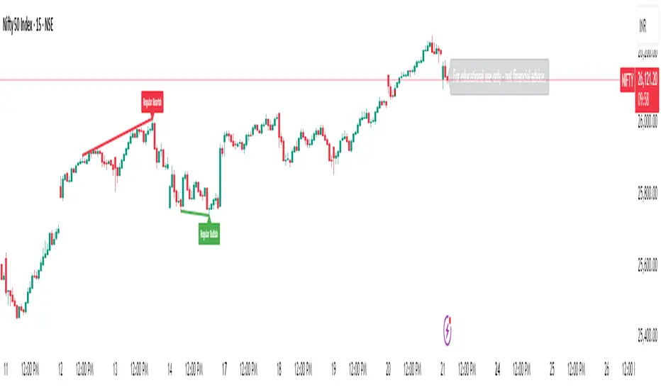
Dynamic Equity Allocation Model"Cash is Trash"? Not Always. Here's Why Science Beats Guesswork.
Every retail trader knows the frustration: you draw support and resistance lines, you spot patterns, you follow market gurus on social media—and still, when the next bear market hits, your portfolio bleeds red. Meanwhile, institutional investors seem to navigate market turbulence with ease, preserving capital when markets crash and participating when they rally. What's their secret?
The answer isn't insider information or access to exotic derivatives. It's systematic, scientifically validated decision-making. While most retail traders rely on subjective chart analysis and emotional reactions, professional portfolio managers use quantitative models that remove emotion from the equation and process multiple streams of market information simultaneously.
This document presents exactly such a system—not a proprietary black box available only to hedge funds, but a fully transparent, academically grounded framework that any serious investor can understand and apply. The Dynamic Equity Allocation Model (DEAM) synthesizes decades of financial research from Nobel laureates and leading academics into a practical tool for tactical asset allocation.
Stop drawing colorful lines on your chart and start thinking like a quant. This isn't about predicting where the market goes next week—it's about systematically adjusting your risk exposure based on what the data actually tells you. When valuations scream danger, when volatility spikes, when credit markets freeze, when multiple warning signals align—that's when cash isn't trash. That's when cash saves your portfolio.
The irony of "cash is trash" rhetoric is that it ignores timing. Yes, being 100% cash for decades would be disastrous. But being 100% equities through every crisis is equally foolish. The sophisticated approach is dynamic: aggressive when conditions favor risk-taking, defensive when they don't. This model shows you how to make that decision systematically, not emotionally.
Whether you're managing your own retirement portfolio or seeking to understand how institutional allocation strategies work, this comprehensive analysis provides the theoretical foundation, mathematical implementation, and practical guidance to elevate your investment approach from amateur to professional.
The choice is yours: keep hoping your chart patterns work out, or start using the same quantitative methods that professionals rely on. The tools are here. The research is cited. The methodology is explained. All you need to do is read, understand, and apply.
The Dynamic Equity Allocation Model (DEAM) is a quantitative framework for systematic allocation between equities and cash, grounded in modern portfolio theory and empirical market research. The model integrates five scientifically validated dimensions of market analysis—market regime, risk metrics, valuation, sentiment, and macroeconomic conditions—to generate dynamic allocation recommendations ranging from 0% to 100% equity exposure. This work documents the theoretical foundations, mathematical implementation, and practical application of this multi-factor approach.
1. Introduction and Theoretical Background
1.1 The Limitations of Static Portfolio Allocation
Traditional portfolio theory, as formulated by Markowitz (1952) in his seminal work "Portfolio Selection," assumes an optimal static allocation where investors distribute their wealth across asset classes according to their risk aversion. This approach rests on the assumption that returns and risks remain constant over time. However, empirical research demonstrates that this assumption does not hold in reality. Fama and French (1989) showed that expected returns vary over time and correlate with macroeconomic variables such as the spread between long-term and short-term interest rates. Campbell and Shiller (1988) demonstrated that the price-earnings ratio possesses predictive power for future stock returns, providing a foundation for dynamic allocation strategies.
The academic literature on tactical asset allocation has evolved considerably over recent decades. Ilmanen (2011) argues in "Expected Returns" that investors can improve their risk-adjusted returns by considering valuation levels, business cycles, and market sentiment. The Dynamic Equity Allocation Model presented here builds on this research tradition and operationalizes these insights into a practically applicable allocation framework.
1.2 Multi-Factor Approaches in Asset Allocation
Modern financial research has shown that different factors capture distinct aspects of market dynamics and together provide a more robust picture of market conditions than individual indicators. Ross (1976) developed the Arbitrage Pricing Theory, a model that employs multiple factors to explain security returns. Following this multi-factor philosophy, DEAM integrates five complementary analytical dimensions, each tapping different information sources and collectively enabling comprehensive market understanding.
2. Data Foundation and Data Quality
2.1 Data Sources Used
The model draws its data exclusively from publicly available market data via the TradingView platform. This transparency and accessibility is a significant advantage over proprietary models that rely on non-public data. The data foundation encompasses several categories of market information, each capturing specific aspects of market dynamics.
First, price data for the S&P 500 Index is obtained through the SPDR S&P 500 ETF (ticker: SPY). The use of a highly liquid ETF instead of the index itself has practical reasons, as ETF data is available in real-time and reflects actual tradability. In addition to closing prices, high, low, and volume data are captured, which are required for calculating advanced volatility measures.
Fundamental corporate metrics are retrieved via TradingView's Financial Data API. These include earnings per share, price-to-earnings ratio, return on equity, debt-to-equity ratio, dividend yield, and share buyback yield. Cochrane (2011) emphasizes in "Presidential Address: Discount Rates" the central importance of valuation metrics for forecasting future returns, making these fundamental data a cornerstone of the model.
Volatility indicators are represented by the CBOE Volatility Index (VIX) and related metrics. The VIX, often referred to as the market's "fear gauge," measures the implied volatility of S&P 500 index options and serves as a proxy for market participants' risk perception. Whaley (2000) describes in "The Investor Fear Gauge" the construction and interpretation of the VIX and its use as a sentiment indicator.
Macroeconomic data includes yield curve information through US Treasury bonds of various maturities and credit risk premiums through the spread between high-yield bonds and risk-free government bonds. These variables capture the macroeconomic conditions and financing conditions relevant for equity valuation. Estrella and Hardouvelis (1991) showed that the shape of the yield curve has predictive power for future economic activity, justifying the inclusion of these data.
2.2 Handling Missing Data
A practical problem when working with financial data is dealing with missing or unavailable values. The model implements a fallback system where a plausible historical average value is stored for each fundamental metric. When current data is unavailable for a specific point in time, this fallback value is used. This approach ensures that the model remains functional even during temporary data outages and avoids systematic biases from missing data. The use of average values as fallback is conservative, as it generates neither overly optimistic nor pessimistic signals.
3. Component 1: Market Regime Detection
3.1 The Concept of Market Regimes
The idea that financial markets exist in different "regimes" or states that differ in their statistical properties has a long tradition in financial science. Hamilton (1989) developed regime-switching models that allow distinguishing between different market states with different return and volatility characteristics. The practical application of this theory consists of identifying the current market state and adjusting portfolio allocation accordingly.
DEAM classifies market regimes using a scoring system that considers three main dimensions: trend strength, volatility level, and drawdown depth. This multidimensional view is more robust than focusing on individual indicators, as it captures various facets of market dynamics. Classification occurs into six distinct regimes: Strong Bull, Bull Market, Neutral, Correction, Bear Market, and Crisis.
3.2 Trend Analysis Through Moving Averages
Moving averages are among the oldest and most widely used technical indicators and have also received attention in academic literature. Brock, Lakonishok, and LeBaron (1992) examined in "Simple Technical Trading Rules and the Stochastic Properties of Stock Returns" the profitability of trading rules based on moving averages and found evidence for their predictive power, although later studies questioned the robustness of these results when considering transaction costs.
The model calculates three moving averages with different time windows: a 20-day average (approximately one trading month), a 50-day average (approximately one quarter), and a 200-day average (approximately one trading year). The relationship of the current price to these averages and the relationship of the averages to each other provide information about trend strength and direction. When the price trades above all three averages and the short-term average is above the long-term, this indicates an established uptrend. The model assigns points based on these constellations, with longer-term trends weighted more heavily as they are considered more persistent.
3.3 Volatility Regimes
Volatility, understood as the standard deviation of returns, is a central concept of financial theory and serves as the primary risk measure. However, research has shown that volatility is not constant but changes over time and occurs in clusters—a phenomenon first documented by Mandelbrot (1963) and later formalized through ARCH and GARCH models (Engle, 1982; Bollerslev, 1986).
DEAM calculates volatility not only through the classic method of return standard deviation but also uses more advanced estimators such as the Parkinson estimator and the Garman-Klass estimator. These methods utilize intraday information (high and low prices) and are more efficient than simple close-to-close volatility estimators. The Parkinson estimator (Parkinson, 1980) uses the range between high and low of a trading day and is based on the recognition that this information reveals more about true volatility than just the closing price difference. The Garman-Klass estimator (Garman and Klass, 1980) extends this approach by additionally considering opening and closing prices.
The calculated volatility is annualized by multiplying it by the square root of 252 (the average number of trading days per year), enabling standardized comparability. The model compares current volatility with the VIX, the implied volatility from option prices. A low VIX (below 15) signals market comfort and increases the regime score, while a high VIX (above 35) indicates market stress and reduces the score. This interpretation follows the empirical observation that elevated volatility is typically associated with falling markets (Schwert, 1989).
3.4 Drawdown Analysis
A drawdown refers to the percentage decline from the highest point (peak) to the lowest point (trough) during a specific period. This metric is psychologically significant for investors as it represents the maximum loss experienced. Calmar (1991) developed the Calmar Ratio, which relates return to maximum drawdown, underscoring the practical relevance of this metric.
The model calculates current drawdown as the percentage distance from the highest price of the last 252 trading days (one year). A drawdown below 3% is considered negligible and maximally increases the regime score. As drawdown increases, the score decreases progressively, with drawdowns above 20% classified as severe and indicating a crisis or bear market regime. These thresholds are empirically motivated by historical market cycles, in which corrections typically encompassed 5-10% drawdowns, bear markets 20-30%, and crises over 30%.
3.5 Regime Classification
Final regime classification occurs through aggregation of scores from trend (40% weight), volatility (30%), and drawdown (30%). The higher weighting of trend reflects the empirical observation that trend-following strategies have historically delivered robust results (Moskowitz, Ooi, and Pedersen, 2012). A total score above 80 signals a strong bull market with established uptrend, low volatility, and minimal losses. At a score below 10, a crisis situation exists requiring defensive positioning. The six regime categories enable a differentiated allocation strategy that not only distinguishes binarily between bullish and bearish but allows gradual gradations.
4. Component 2: Risk-Based Allocation
4.1 Volatility Targeting as Risk Management Approach
The concept of volatility targeting is based on the idea that investors should maximize not returns but risk-adjusted returns. Sharpe (1966, 1994) defined with the Sharpe Ratio the fundamental concept of return per unit of risk, measured as volatility. Volatility targeting goes a step further and adjusts portfolio allocation to achieve constant target volatility. This means that in times of low market volatility, equity allocation is increased, and in times of high volatility, it is reduced.
Moreira and Muir (2017) showed in "Volatility-Managed Portfolios" that strategies that adjust their exposure based on volatility forecasts achieve higher Sharpe Ratios than passive buy-and-hold strategies. DEAM implements this principle by defining a target portfolio volatility (default 12% annualized) and adjusting equity allocation to achieve it. The mathematical foundation is simple: if market volatility is 20% and target volatility is 12%, equity allocation should be 60% (12/20 = 0.6), with the remaining 40% held in cash with zero volatility.
4.2 Market Volatility Calculation
Estimating current market volatility is central to the risk-based allocation approach. The model uses several volatility estimators in parallel and selects the higher value between traditional close-to-close volatility and the Parkinson estimator. This conservative choice ensures the model does not underestimate true volatility, which could lead to excessive risk exposure.
Traditional volatility calculation uses logarithmic returns, as these have mathematically advantageous properties (additive linkage over multiple periods). The logarithmic return is calculated as ln(P_t / P_{t-1}), where P_t is the price at time t. The standard deviation of these returns over a rolling 20-trading-day window is then multiplied by √252 to obtain annualized volatility. This annualization is based on the assumption of independently identically distributed returns, which is an idealization but widely accepted in practice.
The Parkinson estimator uses additional information from the trading range (High minus Low) of each day. The formula is: σ_P = (1/√(4ln2)) × √(1/n × Σln²(H_i/L_i)) × √252, where H_i and L_i are high and low prices. Under ideal conditions, this estimator is approximately five times more efficient than the close-to-close estimator (Parkinson, 1980), as it uses more information per observation.
4.3 Drawdown-Based Position Size Adjustment
In addition to volatility targeting, the model implements drawdown-based risk control. The logic is that deep market declines often signal further losses and therefore justify exposure reduction. This behavior corresponds with the concept of path-dependent risk tolerance: investors who have already suffered losses are typically less willing to take additional risk (Kahneman and Tversky, 1979).
The model defines a maximum portfolio drawdown as a target parameter (default 15%). Since portfolio volatility and portfolio drawdown are proportional to equity allocation (assuming cash has neither volatility nor drawdown), allocation-based control is possible. For example, if the market exhibits a 25% drawdown and target portfolio drawdown is 15%, equity allocation should be at most 60% (15/25).
4.4 Dynamic Risk Adjustment
An advanced feature of DEAM is dynamic adjustment of risk-based allocation through a feedback mechanism. The model continuously estimates what actual portfolio volatility and portfolio drawdown would result at the current allocation. If risk utilization (ratio of actual to target risk) exceeds 1.0, allocation is reduced by an adjustment factor that grows exponentially with overutilization. This implements a form of dynamic feedback that avoids overexposure.
Mathematically, a risk adjustment factor r_adjust is calculated: if risk utilization u > 1, then r_adjust = exp(-0.5 × (u - 1)). This exponential function ensures that moderate overutilization is gently corrected, while strong overutilization triggers drastic reductions. The factor 0.5 in the exponent was empirically calibrated to achieve a balanced ratio between sensitivity and stability.
5. Component 3: Valuation Analysis
5.1 Theoretical Foundations of Fundamental Valuation
DEAM's valuation component is based on the fundamental premise that the intrinsic value of a security is determined by its future cash flows and that deviations between market price and intrinsic value are eventually corrected. Graham and Dodd (1934) established in "Security Analysis" the basic principles of fundamental analysis that remain relevant today. Translated into modern portfolio context, this means that markets with high valuation metrics (high price-earnings ratios) should have lower expected returns than cheaply valued markets.
Campbell and Shiller (1988) developed the Cyclically Adjusted P/E Ratio (CAPE), which smooths earnings over a full business cycle. Their empirical analysis showed that this ratio has significant predictive power for 10-year returns. Asness, Moskowitz, and Pedersen (2013) demonstrated in "Value and Momentum Everywhere" that value effects exist not only in individual stocks but also in asset classes and markets.
5.2 Equity Risk Premium as Central Valuation Metric
The Equity Risk Premium (ERP) is defined as the expected excess return of stocks over risk-free government bonds. It is the theoretical heart of valuation analysis, as it represents the compensation investors demand for bearing equity risk. Damodaran (2012) discusses in "Equity Risk Premiums: Determinants, Estimation and Implications" various methods for ERP estimation.
DEAM calculates ERP not through a single method but combines four complementary approaches with different weights. This multi-method strategy increases estimation robustness and avoids dependence on single, potentially erroneous inputs.
The first method (35% weight) uses earnings yield, calculated as 1/P/E or directly from operating earnings data, and subtracts the 10-year Treasury yield. This method follows Fed Model logic (Yardeni, 2003), although this model has theoretical weaknesses as it does not consistently treat inflation (Asness, 2003).
The second method (30% weight) extends earnings yield by share buyback yield. Share buybacks are a form of capital return to shareholders and increase value per share. Boudoukh et al. (2007) showed in "The Total Shareholder Yield" that the sum of dividend yield and buyback yield is a better predictor of future returns than dividend yield alone.
The third method (20% weight) implements the Gordon Growth Model (Gordon, 1962), which models stock value as the sum of discounted future dividends. Under constant growth g assumption: Expected Return = Dividend Yield + g. The model estimates sustainable growth as g = ROE × (1 - Payout Ratio), where ROE is return on equity and payout ratio is the ratio of dividends to earnings. This formula follows from equity theory: unretained earnings are reinvested at ROE and generate additional earnings growth.
The fourth method (15% weight) combines total shareholder yield (Dividend + Buybacks) with implied growth derived from revenue growth. This method considers that companies with strong revenue growth should generate higher future earnings, even if current valuations do not yet fully reflect this.
The final ERP is the weighted average of these four methods. A high ERP (above 4%) signals attractive valuations and increases the valuation score to 95 out of 100 possible points. A negative ERP, where stocks have lower expected returns than bonds, results in a minimal score of 10.
5.3 Quality Adjustments to Valuation
Valuation metrics alone can be misleading if not interpreted in the context of company quality. A company with a low P/E may be cheap or fundamentally problematic. The model therefore implements quality adjustments based on growth, profitability, and capital structure.
Revenue growth above 10% annually adds 10 points to the valuation score, moderate growth above 5% adds 5 points. This adjustment reflects that growth has independent value (Modigliani and Miller, 1961, extended by later growth theory). Net margin above 15% signals pricing power and operational efficiency and increases the score by 5 points, while low margins below 8% indicate competitive pressure and subtract 5 points.
Return on equity (ROE) above 20% characterizes outstanding capital efficiency and increases the score by 5 points. Piotroski (2000) showed in "Value Investing: The Use of Historical Financial Statement Information" that fundamental quality signals such as high ROE can improve the performance of value strategies.
Capital structure is evaluated through the debt-to-equity ratio. A conservative ratio below 1.0 multiplies the valuation score by 1.2, while high leverage above 2.0 applies a multiplier of 0.8. This adjustment reflects that high debt constrains financial flexibility and can become problematic in crisis times (Korteweg, 2010).
6. Component 4: Sentiment Analysis
6.1 The Role of Sentiment in Financial Markets
Investor sentiment, defined as the collective psychological attitude of market participants, influences asset prices independently of fundamental data. Baker and Wurgler (2006, 2007) developed a sentiment index and showed that periods of high sentiment are followed by overvaluations that later correct. This insight justifies integrating a sentiment component into allocation decisions.
Sentiment is difficult to measure directly but can be proxied through market indicators. The VIX is the most widely used sentiment indicator, as it aggregates implied volatility from option prices. High VIX values reflect elevated uncertainty and risk aversion, while low values signal market comfort. Whaley (2009) refers to the VIX as the "Investor Fear Gauge" and documents its role as a contrarian indicator: extremely high values typically occur at market bottoms, while low values occur at tops.
6.2 VIX-Based Sentiment Assessment
DEAM uses statistical normalization of the VIX by calculating the Z-score: z = (VIX_current - VIX_average) / VIX_standard_deviation. The Z-score indicates how many standard deviations the current VIX is from the historical average. This approach is more robust than absolute thresholds, as it adapts to the average volatility level, which can vary over longer periods.
A Z-score below -1.5 (VIX is 1.5 standard deviations below average) signals exceptionally low risk perception and adds 40 points to the sentiment score. This may seem counterintuitive—shouldn't low fear be bullish? However, the logic follows the contrarian principle: when no one is afraid, everyone is already invested, and there is limited further upside potential (Zweig, 1973). Conversely, a Z-score above 1.5 (extreme fear) adds -40 points, reflecting market panic but simultaneously suggesting potential buying opportunities.
6.3 VIX Term Structure as Sentiment Signal
The VIX term structure provides additional sentiment information. Normally, the VIX trades in contango, meaning longer-term VIX futures have higher prices than short-term. This reflects that short-term volatility is currently known, while long-term volatility is more uncertain and carries a risk premium. The model compares the VIX with VIX9D (9-day volatility) and identifies backwardation (VIX > 1.05 × VIX9D) and steep backwardation (VIX > 1.15 × VIX9D).
Backwardation occurs when short-term implied volatility is higher than longer-term, which typically happens during market stress. Investors anticipate immediate turbulence but expect calming. Psychologically, this reflects acute fear. The model subtracts 15 points for backwardation and 30 for steep backwardation, as these constellations signal elevated risk. Simon and Wiggins (2001) analyzed the VIX futures curve and showed that backwardation is associated with market declines.
6.4 Safe-Haven Flows
During crisis times, investors flee from risky assets into safe havens: gold, US dollar, and Japanese yen. This "flight to quality" is a sentiment signal. The model calculates the performance of these assets relative to stocks over the last 20 trading days. When gold or the dollar strongly rise while stocks fall, this indicates elevated risk aversion.
The safe-haven component is calculated as the difference between safe-haven performance and stock performance. Positive values (safe havens outperform) subtract up to 20 points from the sentiment score, negative values (stocks outperform) add up to 10 points. The asymmetric treatment (larger deduction for risk-off than bonus for risk-on) reflects that risk-off movements are typically sharper and more informative than risk-on phases.
Baur and Lucey (2010) examined safe-haven properties of gold and showed that gold indeed exhibits negative correlation with stocks during extreme market movements, confirming its role as crisis protection.
7. Component 5: Macroeconomic Analysis
7.1 The Yield Curve as Economic Indicator
The yield curve, represented as yields of government bonds of various maturities, contains aggregated expectations about future interest rates, inflation, and economic growth. The slope of the yield curve has remarkable predictive power for recessions. Estrella and Mishkin (1998) showed that an inverted yield curve (short-term rates higher than long-term) predicts recessions with high reliability. This is because inverted curves reflect restrictive monetary policy: the central bank raises short-term rates to combat inflation, dampening economic activity.
DEAM calculates two spread measures: the 2-year-minus-10-year spread and the 3-month-minus-10-year spread. A steep, positive curve (spreads above 1.5% and 2% respectively) signals healthy growth expectations and generates the maximum yield curve score of 40 points. A flat curve (spreads near zero) reduces the score to 20 points. An inverted curve (negative spreads) is particularly alarming and results in only 10 points.
The choice of two different spreads increases analysis robustness. The 2-10 spread is most established in academic literature, while the 3M-10Y spread is often considered more sensitive, as the 3-month rate directly reflects current monetary policy (Ang, Piazzesi, and Wei, 2006).
7.2 Credit Conditions and Spreads
Credit spreads—the yield difference between risky corporate bonds and safe government bonds—reflect risk perception in the credit market. Gilchrist and Zakrajšek (2012) constructed an "Excess Bond Premium" that measures the component of credit spreads not explained by fundamentals and showed this is a predictor of future economic activity and stock returns.
The model approximates credit spread by comparing the yield of high-yield bond ETFs (HYG) with investment-grade bond ETFs (LQD). A narrow spread below 200 basis points signals healthy credit conditions and risk appetite, contributing 30 points to the macro score. Very wide spreads above 1000 basis points (as during the 2008 financial crisis) signal credit crunch and generate zero points.
Additionally, the model evaluates whether "flight to quality" is occurring, identified through strong performance of Treasury bonds (TLT) with simultaneous weakness in high-yield bonds. This constellation indicates elevated risk aversion and reduces the credit conditions score.
7.3 Financial Stability at Corporate Level
While the yield curve and credit spreads reflect macroeconomic conditions, financial stability evaluates the health of companies themselves. The model uses the aggregated debt-to-equity ratio and return on equity of the S&P 500 as proxies for corporate health.
A low leverage level below 0.5 combined with high ROE above 15% signals robust corporate balance sheets and generates 20 points. This combination is particularly valuable as it represents both defensive strength (low debt means crisis resistance) and offensive strength (high ROE means earnings power). High leverage above 1.5 generates only 5 points, as it implies vulnerability to interest rate increases and recessions.
Korteweg (2010) showed in "The Net Benefits to Leverage" that optimal debt maximizes firm value, but excessive debt increases distress costs. At the aggregated market level, high debt indicates fragilities that can become problematic during stress phases.
8. Component 6: Crisis Detection
8.1 The Need for Systematic Crisis Detection
Financial crises are rare but extremely impactful events that suspend normal statistical relationships. During normal market volatility, diversified portfolios and traditional risk management approaches function, but during systemic crises, seemingly independent assets suddenly correlate strongly, and losses exceed historical expectations (Longin and Solnik, 2001). This justifies a separate crisis detection mechanism that operates independently of regular allocation components.
Reinhart and Rogoff (2009) documented in "This Time Is Different: Eight Centuries of Financial Folly" recurring patterns in financial crises: extreme volatility, massive drawdowns, credit market dysfunction, and asset price collapse. DEAM operationalizes these patterns into quantifiable crisis indicators.
8.2 Multi-Signal Crisis Identification
The model uses a counter-based approach where various stress signals are identified and aggregated. This methodology is more robust than relying on a single indicator, as true crises typically occur simultaneously across multiple dimensions. A single signal may be a false alarm, but the simultaneous presence of multiple signals increases confidence.
The first indicator is a VIX above the crisis threshold (default 40), adding one point. A VIX above 60 (as in 2008 and March 2020) adds two additional points, as such extreme values are historically very rare. This tiered approach captures the intensity of volatility.
The second indicator is market drawdown. A drawdown above 15% adds one point, as corrections of this magnitude can be potential harbingers of larger crises. A drawdown above 25% adds another point, as historical bear markets typically encompass 25-40% drawdowns.
The third indicator is credit market spreads above 500 basis points, adding one point. Such wide spreads occur only during significant credit market disruptions, as in 2008 during the Lehman crisis.
The fourth indicator identifies simultaneous losses in stocks and bonds. Normally, Treasury bonds act as a hedge against equity risk (negative correlation), but when both fall simultaneously, this indicates systemic liquidity problems or inflation/stagflation fears. The model checks whether both SPY and TLT have fallen more than 10% and 5% respectively over 5 trading days, adding two points.
The fifth indicator is a volume spike combined with negative returns. Extreme trading volumes (above twice the 20-day average) with falling prices signal panic selling. This adds one point.
A crisis situation is diagnosed when at least 3 indicators trigger, a severe crisis at 5 or more indicators. These thresholds were calibrated through historical backtesting to identify true crises (2008, 2020) without generating excessive false alarms.
8.3 Crisis-Based Allocation Override
When a crisis is detected, the system overrides the normal allocation recommendation and caps equity allocation at maximum 25%. In a severe crisis, the cap is set at 10%. This drastic defensive posture follows the empirical observation that crises typically require time to develop and that early reduction can avoid substantial losses (Faber, 2007).
This override logic implements a "safety first" principle: in situations of existential danger to the portfolio, capital preservation becomes the top priority. Roy (1952) formalized this approach in "Safety First and the Holding of Assets," arguing that investors should primarily minimize ruin probability.
9. Integration and Final Allocation Calculation
9.1 Component Weighting
The final allocation recommendation emerges through weighted aggregation of the five components. The standard weighting is: Market Regime 35%, Risk Management 25%, Valuation 20%, Sentiment 15%, Macro 5%. These weights reflect both theoretical considerations and empirical backtesting results.
The highest weighting of market regime is based on evidence that trend-following and momentum strategies have delivered robust results across various asset classes and time periods (Moskowitz, Ooi, and Pedersen, 2012). Current market momentum is highly informative for the near future, although it provides no information about long-term expectations.
The substantial weighting of risk management (25%) follows from the central importance of risk control. Wealth preservation is the foundation of long-term wealth creation, and systematic risk management is demonstrably value-creating (Moreira and Muir, 2017).
The valuation component receives 20% weight, based on the long-term mean reversion of valuation metrics. While valuation has limited short-term predictive power (bull and bear markets can begin at any valuation), the long-term relationship between valuation and returns is robustly documented (Campbell and Shiller, 1988).
Sentiment (15%) and Macro (5%) receive lower weights, as these factors are subtler and harder to measure. Sentiment is valuable as a contrarian indicator at extremes but less informative in normal ranges. Macro variables such as the yield curve have strong predictive power for recessions, but the transmission from recessions to stock market performance is complex and temporally variable.
9.2 Model Type Adjustments
DEAM allows users to choose between four model types: Conservative, Balanced, Aggressive, and Adaptive. This choice modifies the final allocation through additive adjustments.
Conservative mode subtracts 10 percentage points from allocation, resulting in consistently more cautious positioning. This is suitable for risk-averse investors or those with limited investment horizons. Aggressive mode adds 10 percentage points, suitable for risk-tolerant investors with long horizons.
Adaptive mode implements procyclical adjustment based on short-term momentum: if the market has risen more than 5% in the last 20 days, 5 percentage points are added; if it has declined more than 5%, 5 points are subtracted. This logic follows the observation that short-term momentum persists (Jegadeesh and Titman, 1993), but the moderate size of adjustment avoids excessive timing bets.
Balanced mode makes no adjustment and uses raw model output. This neutral setting is suitable for investors who wish to trust model recommendations unchanged.
9.3 Smoothing and Stability
The allocation resulting from aggregation undergoes final smoothing through a simple moving average over 3 periods. This smoothing is crucial for model practicality, as it reduces frequent trading and thus transaction costs. Without smoothing, the model could fluctuate between adjacent allocations with every small input change.
The choice of 3 periods as smoothing window is a compromise between responsiveness and stability. Longer smoothing would excessively delay signals and impede response to true regime changes. Shorter or no smoothing would allow too much noise. Empirical tests showed that 3-period smoothing offers an optimal ratio between these goals.
10. Visualization and Interpretation
10.1 Main Output: Equity Allocation
DEAM's primary output is a time series from 0 to 100 representing the recommended percentage allocation to equities. This representation is intuitive: 100% means full investment in stocks (specifically: an S&P 500 ETF), 0% means complete cash position, and intermediate values correspond to mixed portfolios. A value of 60% means, for example: invest 60% of wealth in SPY, hold 40% in money market instruments or cash.
The time series is color-coded to enable quick visual interpretation. Green shades represent high allocations (above 80%, bullish), red shades low allocations (below 20%, bearish), and neutral colors middle allocations. The chart background is dynamically colored based on the signal, enhancing readability in different market phases.
10.2 Dashboard Metrics
A tabular dashboard presents key metrics compactly. This includes current allocation, cash allocation (complement), an aggregated signal (BULLISH/NEUTRAL/BEARISH), current market regime, VIX level, market drawdown, and crisis status.
Additionally, fundamental metrics are displayed: P/E Ratio, Equity Risk Premium, Return on Equity, Debt-to-Equity Ratio, and Total Shareholder Yield. This transparency allows users to understand model decisions and form their own assessments.
Component scores (Regime, Risk, Valuation, Sentiment, Macro) are also displayed, each normalized on a 0-100 scale. This shows which factors primarily drive the current recommendation. If, for example, the Risk score is very low (20) while other scores are moderate (50-60), this indicates that risk management considerations are pulling allocation down.
10.3 Component Breakdown (Optional)
Advanced users can display individual components as separate lines in the chart. This enables analysis of component dynamics: do all components move synchronously, or are there divergences? Divergences can be particularly informative. If, for example, the market regime is bullish (high score) but the valuation component is very negative, this signals an overbought market not fundamentally supported—a classic "bubble warning."
This feature is disabled by default to keep the chart clean but can be activated for deeper analysis.
10.4 Confidence Bands
The model optionally displays uncertainty bands around the main allocation line. These are calculated as ±1 standard deviation of allocation over a rolling 20-period window. Wide bands indicate high volatility of model recommendations, suggesting uncertain market conditions. Narrow bands indicate stable recommendations.
This visualization implements a concept of epistemic uncertainty—uncertainty about the model estimate itself, not just market volatility. In phases where various indicators send conflicting signals, the allocation recommendation becomes more volatile, manifesting in wider bands. Users can understand this as a warning to act more cautiously or consult alternative information sources.
11. Alert System
11.1 Allocation Alerts
DEAM implements an alert system that notifies users of significant events. Allocation alerts trigger when smoothed allocation crosses certain thresholds. An alert is generated when allocation reaches 80% (from below), signaling strong bullish conditions. Another alert triggers when allocation falls to 20%, indicating defensive positioning.
These thresholds are not arbitrary but correspond with boundaries between model regimes. An allocation of 80% roughly corresponds to a clear bull market regime, while 20% corresponds to a bear market regime. Alerts at these points are therefore informative about fundamental regime shifts.
11.2 Crisis Alerts
Separate alerts trigger upon detection of crisis and severe crisis. These alerts have highest priority as they signal large risks. A crisis alert should prompt investors to review their portfolio and potentially take defensive measures beyond the automatic model recommendation (e.g., hedging through put options, rebalancing to more defensive sectors).
11.3 Regime Change Alerts
An alert triggers upon change of market regime (e.g., from Neutral to Correction, or from Bull Market to Strong Bull). Regime changes are highly informative events that typically entail substantial allocation changes. These alerts enable investors to proactively respond to changes in market dynamics.
11.4 Risk Breach Alerts
A specialized alert triggers when actual portfolio risk utilization exceeds target parameters by 20%. This is a warning signal that the risk management system is reaching its limits, possibly because market volatility is rising faster than allocation can be reduced. In such situations, investors should consider manual interventions.
12. Practical Application and Limitations
12.1 Portfolio Implementation
DEAM generates a recommendation for allocation between equities (S&P 500) and cash. Implementation by an investor can take various forms. The most direct method is using an S&P 500 ETF (e.g., SPY, VOO) for equity allocation and a money market fund or savings account for cash allocation.
A rebalancing strategy is required to synchronize actual allocation with model recommendation. Two approaches are possible: (1) rule-based rebalancing at every 10% deviation between actual and target, or (2) time-based monthly rebalancing. Both have trade-offs between responsiveness and transaction costs. Empirical evidence (Jaconetti, Kinniry, and Zilbering, 2010) suggests rebalancing frequency has moderate impact on performance, and investors should optimize based on their transaction costs.
12.2 Adaptation to Individual Preferences
The model offers numerous adjustment parameters. Component weights can be modified if investors place more or less belief in certain factors. A fundamentally-oriented investor might increase valuation weight, while a technical trader might increase regime weight.
Risk target parameters (target volatility, max drawdown) should be adapted to individual risk tolerance. Younger investors with long investment horizons can choose higher target volatility (15-18%), while retirees may prefer lower volatility (8-10%). This adjustment systematically shifts average equity allocation.
Crisis thresholds can be adjusted based on preference for sensitivity versus specificity of crisis detection. Lower thresholds (e.g., VIX > 35 instead of 40) increase sensitivity (more crises are detected) but reduce specificity (more false alarms). Higher thresholds have the reverse effect.
12.3 Limitations and Disclaimers
DEAM is based on historical relationships between indicators and market performance. There is no guarantee these relationships will persist in the future. Structural changes in markets (e.g., through regulation, technology, or central bank policy) can break established patterns. This is the fundamental problem of induction in financial science (Taleb, 2007).
The model is optimized for US equities (S&P 500). Application to other markets (international stocks, bonds, commodities) would require recalibration. The indicators and thresholds are specific to the statistical properties of the US equity market.
The model cannot eliminate losses. Even with perfect crisis prediction, an investor following the model would lose money in bear markets—just less than a buy-and-hold investor. The goal is risk-adjusted performance improvement, not risk elimination.
Transaction costs are not modeled. In practice, spreads, commissions, and taxes reduce net returns. Frequent trading can cause substantial costs. Model smoothing helps minimize this, but users should consider their specific cost situation.
The model reacts to information; it does not anticipate it. During sudden shocks (e.g., 9/11, COVID-19 lockdowns), the model can only react after price movements, not before. This limitation is inherent to all reactive systems.
12.4 Relationship to Other Strategies
DEAM is a tactical asset allocation approach and should be viewed as a complement, not replacement, for strategic asset allocation. Brinson, Hood, and Beebower (1986) showed in their influential study "Determinants of Portfolio Performance" that strategic asset allocation (long-term policy allocation) explains the majority of portfolio performance, but this leaves room for tactical adjustments based on market timing.
The model can be combined with value and momentum strategies at the individual stock level. While DEAM controls overall market exposure, within-equity decisions can be optimized through stock-picking models. This separation between strategic (market exposure) and tactical (stock selection) levels follows classical portfolio theory.
The model does not replace diversification across asset classes. A complete portfolio should also include bonds, international stocks, real estate, and alternative investments. DEAM addresses only the US equity allocation decision within a broader portfolio.
13. Scientific Foundation and Evaluation
13.1 Theoretical Consistency
DEAM's components are based on established financial theory and empirical evidence. The market regime component follows from regime-switching models (Hamilton, 1989) and trend-following literature. The risk management component implements volatility targeting (Moreira and Muir, 2017) and modern portfolio theory (Markowitz, 1952). The valuation component is based on discounted cash flow theory and empirical value research (Campbell and Shiller, 1988; Fama and French, 1992). The sentiment component integrates behavioral finance (Baker and Wurgler, 2006). The macro component uses established business cycle indicators (Estrella and Mishkin, 1998).
This theoretical grounding distinguishes DEAM from purely data-mining-based approaches that identify patterns without causal theory. Theory-guided models have greater probability of functioning out-of-sample, as they are based on fundamental mechanisms, not random correlations (Lo and MacKinlay, 1990).
13.2 Empirical Validation
While this document does not present detailed backtest analysis, it should be noted that rigorous validation of a tactical asset allocation model should include several elements:
In-sample testing establishes whether the model functions at all in the data on which it was calibrated. Out-of-sample testing is crucial: the model should be tested in time periods not used for development. Walk-forward analysis, where the model is successively trained on rolling windows and tested in the next window, approximates real implementation.
Performance metrics should be risk-adjusted. Pure return consideration is misleading, as higher returns often only compensate for higher risk. Sharpe Ratio, Sortino Ratio, Calmar Ratio, and Maximum Drawdown are relevant metrics. Comparison with benchmarks (Buy-and-Hold S&P 500, 60/40 Stock/Bond portfolio) contextualizes performance.
Robustness checks test sensitivity to parameter variation. If the model only functions at specific parameter settings, this indicates overfitting. Robust models show consistent performance over a range of plausible parameters.
13.3 Comparison with Existing Literature
DEAM fits into the broader literature on tactical asset allocation. Faber (2007) presented a simple momentum-based timing system that goes long when the market is above its 10-month average, otherwise cash. This simple system avoided large drawdowns in bear markets. DEAM can be understood as a sophistication of this approach that integrates multiple information sources.
Ilmanen (2011) discusses various timing factors in "Expected Returns" and argues for multi-factor approaches. DEAM operationalizes this philosophy. Asness, Moskowitz, and Pedersen (2013) showed that value and momentum effects work across asset classes, justifying cross-asset application of regime and valuation signals.
Ang (2014) emphasizes in "Asset Management: A Systematic Approach to Factor Investing" the importance of systematic, rule-based approaches over discretionary decisions. DEAM is fully systematic and eliminates emotional biases that plague individual investors (overconfidence, hindsight bias, loss aversion).
References
Ang, A. (2014) *Asset Management: A Systematic Approach to Factor Investing*. Oxford: Oxford University Press.
Ang, A., Piazzesi, M. and Wei, M. (2006) 'What does the yield curve tell us about GDP growth?', *Journal of Econometrics*, 131(1-2), pp. 359-403.
Asness, C.S. (2003) 'Fight the Fed Model', *The Journal of Portfolio Management*, 30(1), pp. 11-24.
Asness, C.S., Moskowitz, T.J. and Pedersen, L.H. (2013) 'Value and Momentum Everywhere', *The Journal of Finance*, 68(3), pp. 929-985.
Baker, M. and Wurgler, J. (2006) 'Investor Sentiment and the Cross-Section of Stock Returns', *The Journal of Finance*, 61(4), pp. 1645-1680.
Baker, M. and Wurgler, J. (2007) 'Investor Sentiment in the Stock Market', *Journal of Economic Perspectives*, 21(2), pp. 129-152.
Baur, D.G. and Lucey, B.M. (2010) 'Is Gold a Hedge or a Safe Haven? An Analysis of Stocks, Bonds and Gold', *Financial Review*, 45(2), pp. 217-229.
Bollerslev, T. (1986) 'Generalized Autoregressive Conditional Heteroskedasticity', *Journal of Econometrics*, 31(3), pp. 307-327.
Boudoukh, J., Michaely, R., Richardson, M. and Roberts, M.R. (2007) 'On the Importance of Measuring Payout Yield: Implications for Empirical Asset Pricing', *The Journal of Finance*, 62(2), pp. 877-915.
Brinson, G.P., Hood, L.R. and Beebower, G.L. (1986) 'Determinants of Portfolio Performance', *Financial Analysts Journal*, 42(4), pp. 39-44.
Brock, W., Lakonishok, J. and LeBaron, B. (1992) 'Simple Technical Trading Rules and the Stochastic Properties of Stock Returns', *The Journal of Finance*, 47(5), pp. 1731-1764.
Calmar, T.W. (1991) 'The Calmar Ratio', *Futures*, October issue.
Campbell, J.Y. and Shiller, R.J. (1988) 'The Dividend-Price Ratio and Expectations of Future Dividends and Discount Factors', *Review of Financial Studies*, 1(3), pp. 195-228.
Cochrane, J.H. (2011) 'Presidential Address: Discount Rates', *The Journal of Finance*, 66(4), pp. 1047-1108.
Damodaran, A. (2012) *Equity Risk Premiums: Determinants, Estimation and Implications*. Working Paper, Stern School of Business.
Engle, R.F. (1982) 'Autoregressive Conditional Heteroskedasticity with Estimates of the Variance of United Kingdom Inflation', *Econometrica*, 50(4), pp. 987-1007.
Estrella, A. and Hardouvelis, G.A. (1991) 'The Term Structure as a Predictor of Real Economic Activity', *The Journal of Finance*, 46(2), pp. 555-576.
Estrella, A. and Mishkin, F.S. (1998) 'Predicting U.S. Recessions: Financial Variables as Leading Indicators', *Review of Economics and Statistics*, 80(1), pp. 45-61.
Faber, M.T. (2007) 'A Quantitative Approach to Tactical Asset Allocation', *The Journal of Wealth Management*, 9(4), pp. 69-79.
Fama, E.F. and French, K.R. (1989) 'Business Conditions and Expected Returns on Stocks and Bonds', *Journal of Financial Economics*, 25(1), pp. 23-49.
Fama, E.F. and French, K.R. (1992) 'The Cross-Section of Expected Stock Returns', *The Journal of Finance*, 47(2), pp. 427-465.
Garman, M.B. and Klass, M.J. (1980) 'On the Estimation of Security Price Volatilities from Historical Data', *Journal of Business*, 53(1), pp. 67-78.
Gilchrist, S. and Zakrajšek, E. (2012) 'Credit Spreads and Business Cycle Fluctuations', *American Economic Review*, 102(4), pp. 1692-1720.
Gordon, M.J. (1962) *The Investment, Financing, and Valuation of the Corporation*. Homewood: Irwin.
Graham, B. and Dodd, D.L. (1934) *Security Analysis*. New York: McGraw-Hill.
Hamilton, J.D. (1989) 'A New Approach to the Economic Analysis of Nonstationary Time Series and the Business Cycle', *Econometrica*, 57(2), pp. 357-384.
Ilmanen, A. (2011) *Expected Returns: An Investor's Guide to Harvesting Market Rewards*. Chichester: Wiley.
Jaconetti, C.M., Kinniry, F.M. and Zilbering, Y. (2010) 'Best Practices for Portfolio Rebalancing', *Vanguard Research Paper*.
Jegadeesh, N. and Titman, S. (1993) 'Returns to Buying Winners and Selling Losers: Implications for Stock Market Efficiency', *The Journal of Finance*, 48(1), pp. 65-91.
Kahneman, D. and Tversky, A. (1979) 'Prospect Theory: An Analysis of Decision under Risk', *Econometrica*, 47(2), pp. 263-292.
Korteweg, A. (2010) 'The Net Benefits to Leverage', *The Journal of Finance*, 65(6), pp. 2137-2170.
Lo, A.W. and MacKinlay, A.C. (1990) 'Data-Snooping Biases in Tests of Financial Asset Pricing Models', *Review of Financial Studies*, 3(3), pp. 431-467.
Longin, F. and Solnik, B. (2001) 'Extreme Correlation of International Equity Markets', *The Journal of Finance*, 56(2), pp. 649-676.
Mandelbrot, B. (1963) 'The Variation of Certain Speculative Prices', *The Journal of Business*, 36(4), pp. 394-419.
Markowitz, H. (1952) 'Portfolio Selection', *The Journal of Finance*, 7(1), pp. 77-91.
Modigliani, F. and Miller, M.H. (1961) 'Dividend Policy, Growth, and the Valuation of Shares', *The Journal of Business*, 34(4), pp. 411-433.
Moreira, A. and Muir, T. (2017) 'Volatility-Managed Portfolios', *The Journal of Finance*, 72(4), pp. 1611-1644.
Moskowitz, T.J., Ooi, Y.H. and Pedersen, L.H. (2012) 'Time Series Momentum', *Journal of Financial Economics*, 104(2), pp. 228-250.
Parkinson, M. (1980) 'The Extreme Value Method for Estimating the Variance of the Rate of Return', *Journal of Business*, 53(1), pp. 61-65.
Piotroski, J.D. (2000) 'Value Investing: The Use of Historical Financial Statement Information to Separate Winners from Losers', *Journal of Accounting Research*, 38, pp. 1-41.
Reinhart, C.M. and Rogoff, K.S. (2009) *This Time Is Different: Eight Centuries of Financial Folly*. Princeton: Princeton University Press.
Ross, S.A. (1976) 'The Arbitrage Theory of Capital Asset Pricing', *Journal of Economic Theory*, 13(3), pp. 341-360.
Roy, A.D. (1952) 'Safety First and the Holding of Assets', *Econometrica*, 20(3), pp. 431-449.
Schwert, G.W. (1989) 'Why Does Stock Market Volatility Change Over Time?', *The Journal of Finance*, 44(5), pp. 1115-1153.
Sharpe, W.F. (1966) 'Mutual Fund Performance', *The Journal of Business*, 39(1), pp. 119-138.
Sharpe, W.F. (1994) 'The Sharpe Ratio', *The Journal of Portfolio Management*, 21(1), pp. 49-58.
Simon, D.P. and Wiggins, R.A. (2001) 'S&P Futures Returns and Contrary Sentiment Indicators', *Journal of Futures Markets*, 21(5), pp. 447-462.
Taleb, N.N. (2007) *The Black Swan: The Impact of the Highly Improbable*. New York: Random House.
Whaley, R.E. (2000) 'The Investor Fear Gauge', *The Journal of Portfolio Management*, 26(3), pp. 12-17.
Whaley, R.E. (2009) 'Understanding the VIX', *The Journal of Portfolio Management*, 35(3), pp. 98-105.
Yardeni, E. (2003) 'Stock Valuation Models', *Topical Study*, 51, Yardeni Research.
Zweig, M.E. (1973) 'An Investor Expectations Stock Price Predictive Model Using Closed-End Fund Premiums', *The Journal of Finance*, 28(1), pp. 67-78.

PriceActionLibrary "PriceAction"
Hi all!
This library will help you to plot the market structure and liquidity. By now, the only part in the price action section is liquidity, but I plan to add more later on. The market structure will be split into two parts, 'Internal' and 'Swing' with separate pivot lengths. For these two trends it will show you:
• Break of structure (BOS)
• Change of character (CHoCH/CHoCH+) (mandatory)
• Equal high/low (EQH/EQL)
It's inspired by "Smart Money Concepts (SMC) " by LuxAlgo.
This library is now the same code as the code in my library 'MarketStructure', but it has evolved into a more price action oriented library than just a market structure library. This is more accurate and I will continue working on this library to keep it growing.
This code does not provide any examples, but you can look at my indicators 'Market structure' () and 'Order blocks' (), where I use the 'MarketStructure' library (which is the same code).
Market structure
Both of these market structures can be enabled/disabled by setting them to 'na'. The pivots lengths can be configured separately. The pivots found will be the 'base' of and will show you when price breaks it. When that happens a break of structure or a change of character will be created. The latest 5 pivots found within the current trends will be kept to take action on. They are cleared on a change of character, so nothing (break of structures or change of characters) can happen on pivots before a trend change. The internal market structure is shown with dashed lines and swing market structure is shown with solid lines.
Labels for a change of character can have either the text 'CHoCH' or 'CHoCH+'. A Change of Character plus is formed when price fails to form a higher high or a lower low before reversing. Note that a pivot that is created after the change of character might have a higher high or a lower low, thus not making the break a 'CHoCH+'. This is not changed after the pivot is found but is kept as is.
A break of structure is removed if an earlier pivot within the same trend is broken, i.e. another break of structure (with a longer distance) is created. Like in the images below, the first pivot (in the first image) is removed when an earlier pivot's higher price within the same trend is broken (the second image):
[image [https://www.tradingview.com/x/PRP6YtPA/
Equal high/lows have a configurable color setting and can be configured to be extended to the right. Equal high/lows are only possible if it's not been broken by price. A factor (percentage of width) of the Average True Length (of length 14) that the pivot must be within to to be considered an Equal high/low. Equal highs/lows can be of 2 pivots or more.
You are able to show the pivots that are used. "HH" (higher high), "HL" (higher low), "LH" (lower high), "LL" (lower low) and "H"/"L" (for pivots (high/low) when the trend has changed) are the labels used. There are also labels for break of structures ('BOS') and change of characters ('CHoCH' or 'CHoCH+'). The size of these texts is set in the 'FontSize' setting.
When programming I focused on simplicity and ease of read. I did not focus on performance, I will do so if it's a problem (haven't noticed it is one yet).
You can set alerts for when a change of character, break of structure or an equal high/low (new or an addition to a previously found) happens. The alerts that are fired are on 'once_per_bar_close' to avoid repainting. This has the drawback to alert you when the bar closes.
Price action
The indicator will create lines and zones for spotted liquidity. It will draw a line (with dotted style) at the price level that was liquidated, but it will also draw a zone from that level to the bar that broke the pivot high or low price. If that zone is large the liquidation is big and might be significant. This can be disabled in the settings. You can also change the confirmation candles (that does not close above or below the pivot level) needed after a liquidation and how many pivots back to look at.
The lines and boxes drawn will look like this if the color is orange:
Hope this is of help!
Will draw out the market structure for the disired pivot length.
Liqudity(liquidity)
Will draw liquidity.
Parameters:
liquidity (Liquidity) : The 'PriceAction.Liquidity' object.
Pivot(structure)
Sets the pivots in the structure.
Parameters:
structure (Structure)
PivotLabels(structure)
Draws labels for the pivots found.
Parameters:
structure (Structure)
EqualHighOrLow(structure)
Draws the boxes for equal highs/lows. Also creates labels for the pivots included.
Parameters:
structure (Structure)
BreakOfStructure(structure)
Will create lines when a break of strycture occures.
Parameters:
structure (Structure)
Returns: A boolean that represents if a break of structure was found or not.
ChangeOfCharacter(structure)
Will create lines when a change of character occures. This line will have a label with "CHoCH" or "CHoCH+".
Parameters:
structure (Structure)
Returns: A boolean that represents if a change of character was found or not.
VisualizeCurrent(structure)
Will create a box with a background for between the latest high and low pivots. This can be used as the current trading range (if the pivots broke strucure somehow).
Parameters:
structure (Structure)
StructureBreak
Holds drawings for a structure break.
Fields:
Line (series line) : The line object.
Label (series label) : The label object.
Pivot
Holds all the values for a found pivot.
Fields:
Price (series float) : The price of the pivot.
BarIndex (series int) : The bar_index where the pivot occured.
Type (series int) : The type of the pivot (-1 = low, 1 = high).
Time (series int) : The time where the pivot occured.
BreakOfStructureBroken (series bool) : Sets to true if a break of structure has happened.
LiquidityBroken (series bool) : Sets to true if a liquidity of the price level has happened.
ChangeOfCharacterBroken (series bool) : Sets to true if a change of character has happened.
Structure
Holds all the values for the market structure.
Fields:
LeftLength (series int) : Define the left length of the pivots used.
RightLength (series int) : Define the right length of the pivots used.
Type (series Type) : Set the type of the market structure. Two types can be used, 'internal' and 'swing' (0 = internal, 1 = swing).
Trend (series int) : This will be set internally and can be -1 = downtrend, 1 = uptrend.
EqualPivotsFactor (series float) : Set how the limits are for an equal pivot. This is a factor of the Average True Length (ATR) of length 14. If a low pivot is considered to be equal if it doesn't break the low pivot (is at a lower value) and is inside the previous low pivot + this limit.
ExtendEqualPivotsZones (series bool) : Set to true if you want the equal pivots zones to be extended.
ExtendEqualPivotsStyle (series string) : Set the style of equal pivot zones.
ExtendEqualPivotsColor (series color) : Set the color of equal pivot zones.
EqualHighs (array) : Holds the boxes for zones that contains equal highs.
EqualLows (array) : Holds the boxes for zones that contains equal lows.
BreakOfStructures (array) : Holds all the break of structures within the trend (before a change of character).
Pivots (array) : All the pivots in the current trend, added with the latest first, this is cleared when the trend changes.
FontSize (series int) : Holds the size of the font displayed.
AlertChangeOfCharacter (series bool) : Holds true or false if a change of character should be alerted or not.
AlertBreakOfStructure (series bool) : Holds true or false if a break of structure should be alerted or not.
AlerEqualPivots (series bool) : Holds true or false if equal highs/lows should be alerted or not.
Liquidity
Holds all the values for liquidity.
Fields:
LiquidityPivotsHigh (array) : All high pivots for liquidity.
LiquidityPivotsLow (array) : All low pivots for liquidity.
LiquidityConfirmationBars (series int) : The number of bars to confirm that a liquidity is valid.
LiquidityPivotsLookback (series int) : A number of pivots to look back for.
FontSize (series int) : Holds the size of the font displayed.
PriceAction
Holds all the values for the general price action and the market structures.
Fields:
Liquidity (Liquidity)
Swing (Structure) : Placeholder for all objects used for the swing market structure.
Internal (Structure) : Placeholder for all objects used for the internal market structure.

Fibonacci Retracement levels Automatically D/W/MIndicator Description: Fibonacci Retracement levels Automatically
Fibonacci retracement levels based on the day, week, month High Low range and Fibonacci retracement levels draws automatically .This Pine Script indicator is designed to plot Fibonacci retracement levels based on the high and low prices of a user-selected timeframe (Daily, Weekly, or Monthly). It identifies bullish or bearish candles in the chosen timeframe, draws key price levels, and overlays Fibonacci retracement lines and semi-transparent colored boxes to highlight potential support and resistance zones. The indicator dynamically updates with each new period and extends lines, labels, and boxes to the current bar for real-time visualization. Key Features
1. Timeframe Selection: Users can choose the timeframe for analysis: Daily, Weekly, or Monthly via an input dropdown. The indicator retrieves the open, high, low, and close prices for the selected timeframe using `request.security`.
2. High and Low Tracking : Tracks the highest high and lowest low within the selected timeframe. Stores these values and their corresponding bar indices in arrays (`whigh`, `wlow`, `whighIdx`,`wlowIdx`). Limits the array size to the most recent period to optimize performance.
3. Bullish and Bearish Candle Detection : Identifies whether the previous period’s candle is bullish (`close > open`) or bearish (`close < open`). Uses this to determine the direction for Fibonacci retracement calculations. Bullish candle: Fibonacci levels are drawn from low to high
Bearish candle: Fibonacci levels are drawn from high to low
4. Fibonacci Retracement Levels : Plots Fibonacci levels at 0.236, 0.382, 0.5, 0.618, and 0.786 between the high and low of the period. For bullish candles, levels are calculated from the low (support) to the high (resistance). For bearish candles, levels are calculated from the high (resistance) to the low (support). Each Fibonacci level is drawn as a horizontal line with a unique color:
- 0.236: Blue
- 0.382: Purple
- 0.5: Yellow
- 0.618: Teal
- 0.786: Fuchsia
5. Visual Elements: - High/Low Lines and Labels: Draws a red line and label for the previous period’s high. Draws a green line and label for the previous period’s low. Fibonacci Lines and Labels: Each Fibonacci level has a horizontal line and a label displaying the ratio.
Colored Boxes: Semi-transparent boxes are drawn between consecutive Fibonacci levels (including high and low) to highlight zones.
6. Dynamic Updates:
- At the start of a new period (e.g., new week for Weekly timeframe), the indicator:
- Clears previous Fibonacci lines, labels, and boxes.
- Recalculates the high and low for the new period.
- Redraws lines, labels, and boxes based on the new data.
- Extends all lines, labels, and boxes to the current bar index for real-time tracking.
7. Performance Optimization:
- Deletes old lines, labels, and boxes to prevent clutter.
- Limits the storage of highs and lows to the most recent period.
How It Works
1. Initialization: Defines variables for tracking bullish/bearish candles, lines, labels, and arrays for Fibonacci levels and boxes. Sets up color arrays for Fibonacci lines and boxes with distinct, semi-transparent colors.
2. Data Collection: Fetches the previous period’s OHLC (open, high, low, close) using `request.security`. Detects new periods (e.g., new week or month) using `ta.change(time(tf))`.
3. Fibonacci Calculation: On a new period, stores the high and low prices and their bar indices.
- Identifies the maximum high and minimum low from the stored data. - Calculates Fibonacci levels based on the range (`maxHigh - minLow`) and the direction (bullish or bearish).
4. Drawing:
- Draws high/low lines and labels at the identified price levels. Plots Fibonacci retracement lines and labels for each ratio. Creates semi-transparent boxes between Fibonacci levels to visually distinguish zones.
5. Updates:
- Extends all lines, labels, and boxes to the current bar index when a new period is detected. Clears old Fibonacci elements to avoid overlap and ensure clarity.
Usage
- Purpose: This indicator is useful for traders who use Fibonacci retracement levels to identify potential support and resistance zones in financial markets.
- Application:
- Select the desired timeframe (Daily, Weekly, Monthly) via the input settings.
- The indicator automatically plots the previous period’s high/low and Fibonacci levels on the chart.
- Use the labeled Fibonacci levels and colored boxes to identify key price zones for trading decisions.
- Customization:
- Modify the `timeframe` input to switch between Daily, Weekly, or Monthly analysis.
- Adjust the `fibLineColors` and `fibFillColors` arrays to change the visual appearance of lines and boxes.
- The indicator is designed for use on TradingView with Pine Script.
- The maximum array size for highs/lows is limited to 1 period in this version (can be adjusted by modifying the `array.shift` logic).
- The indicator dynamically updates with each new period, ensuring real-time relevance.
This indicator make educational purpose use only

Enigma Sniper 369The "Enigma Sniper 369" is a custom-built Pine Script indicator designed for TradingView, tailored specifically for forex traders seeking high-probability entries during high-volatility market sessions.
Unlike generic trend-following or scalping tools, this indicator uniquely combines session-based "kill zones" (London and US sessions), momentum-based candle analysis, and an optional EMA trend filter to pinpoint liquidity grabs and reversal opportunities.
Its originality lies in its focus on liquidity hunting—identifying levels where stop losses are likely clustered (around swing highs/lows and wick midpoints)—and providing visual entry zones that are dynamically removed once price breaches them, reducing clutter and focusing on actionable signals.
The name "369" reflects the structured approach of three key components (session timing, candle logic, and trend filter) working in harmony to snipe precise entries.
What It Does
"Enigma Sniper 369" identifies potential buy and sell opportunities by drawing two types of horizontal lines on the chart during user-defined London and US
session kill zones:
Solid Lines: Mark the swing low (for buys) or swing high (for sells) of a trigger candle, indicating a potential entry point where stop losses might be clustered.
Dotted Lines: Mark the 50% level of the candle’s wick (lower wick for buys, upper wick for sells), serving as a secondary confirmation zone for entries or tighter stop-loss placement.
These lines are plotted only when specific candle conditions are met within the kill zones, and they are automatically deleted once the price crosses them, signaling that the liquidity at that level has likely been grabbed. The indicator also includes an optional EMA filter to ensure trades align with the broader trend, reducing false signals in choppy markets.
How It Works
The indicator’s logic is built on a multi-layered approach:
Kill Zone Timing: Trades are only considered during user-defined London and US session hours (e.g., London from 02:00 to 12:00 UTC, as seen in the screenshots). These sessions are known for high volatility and liquidity, making them ideal for capturing institutional moves.
Candle-Based Momentum Logic:
Buy Signal: A candle must close above its midpoint (indicating bullish momentum) and have a lower low than the previous candle (suggesting a potential liquidity grab below the previous swing low). This is expressed as close > (high + low) / 2 and low < low .
Sell Signal: A candle must close below its midpoint (bearish momentum) and have a higher high than the previous candle (indicating a potential liquidity grab above the previous swing high), expressed as close < (high + low) / 2 and high > high .
These conditions ensure the indicator targets candles that break recent structure to hunt stop losses while showing directional momentum.
Optional EMA Filter: A 50-period EMA (customizable) can be enabled to filter signals based on trend direction.
Buy signals are only generated if the EMA is trending upward (ema_value > ema_value ), and sell signals require a downward EMA trend (ema_value < ema_value ). This reduces noise by aligning entries with the broader market trend.
Liquidity Levels and Deletion Logic:
For a buy signal, a solid green line is drawn at the candle’s low, and a dotted green line at the 50% level of the lower wick (from the candle body’s bottom to the low).
For a sell signal, a solid red line is drawn at the candle’s high, and a dotted red line at the 50% level of the upper wick (from the body’s top to the high).
These lines extend to the right until the price crosses them, at which point they are deleted, indicating the liquidity at that level has been taken (e.g., stop losses triggered).
Alerts: The indicator includes alert conditions for buy and sell signals, notifying traders when a new setup is identified.
Underlying Concepts
The indicator is grounded in the concept of liquidity hunting, a strategy often employed by institutional traders. Markets frequently move to levels where stop losses are clustered—typically just beyond swing highs or lows—before reversing in the opposite direction. The "Enigma Sniper 369" targets these moves by identifying candles that break structure (e.g., a lower low or higher high) during high-volatility sessions, suggesting a potential sweep of stop losses. The 50% wick level acts as a secondary confirmation, as this midpoint often represents a zone where tighter stop losses are placed by retail traders. The optional EMA filter adds a trend-following element, ensuring entries are taken in the direction of the broader market momentum, which is particularly useful on lower timeframes like the 15-minute chart shown in the screenshots.
How to Use It
Here’s a step-by-step guide based on the provided usage example on the GBP/USD 15-minute chart:
Setup the Indicator: Add "Enigma Sniper 369" to your TradingView chart. Adjust the London and US session hours to match your timezone (e.g., London from 02:00 to 12:00 UTC, US from 13:00 to 22:00 UTC). Customize the EMA period (default 50) and line styles/colors if desired.
Identify Kill Zones: The indicator highlights the London session in light green and the US session in light purple, as seen in the screenshots. Focus on these periods for signals, as they are the most volatile and likely to produce liquidity grabs.
Wait for a Signal: Look for solid and dotted lines to appear during the kill zones:
Buy Setup: A solid green line at the swing low and a dotted green line at the 50% lower wick level indicate a potential buy. This suggests the market may have grabbed liquidity below the swing low and is now poised to move higher.
Sell Setup: A solid red line at the swing high and a dotted red line at the 50% upper wick level indicate a potential sell, suggesting liquidity was taken above the swing high.
Place Your Trade:
For a buy, set a buy limit order at the dotted green line (50% wick level), as this is a more conservative entry point. Place your stop loss just below the solid green line (swing low) to cover the full swing. For example, in the screenshots, the market retraces to the dotted line at 1.32980 after a liquidity grab below the swing low, triggering a buy limit order.
For a sell, set a sell limit order at the dotted red line, with a stop loss just above the solid red line.
Monitor Price Action: Once the price crosses a line, it is deleted, indicating the liquidity at that level has been taken. In the screenshots, after the buy limit is triggered, the market moves higher, confirming the setup. The caption notes, “The market returns and tags us in long with a buy limit,” highlighting this retracement strategy.
Additional Context: Use the indicator to identify liquidity levels that may be targeted later. For example, the screenshot notes, “If a new session is about to open I will wait for the grab liquidity to go long,” showing how the indicator can be used to anticipate future moves at session opens (e.g., London open at 1.32980).
Risk Management: Always set a stop loss below the swing low (for buys) or above the swing high (for sells) to protect against adverse moves. The 50% wick level helps tighten entries, improving the risk-reward ratio.
Practical Example
On the GBP/USD 15-minute chart, during the London session (02:00 UTC), the indicator identifies a buy setup with a solid green line at 1.32901 (swing low) and a dotted green line at 1.32980 (50% wick level). The market initially dips below the swing low, grabbing liquidity, then retraces to the dotted line, triggering a buy limit order. The price subsequently rises to 1.33404, yielding a profitable trade. The user notes, “The logic is in the last candle it provides new level to go long,” emphasizing the indicator’s ability to identify fresh levels after a liquidity sweep.
Customization Tips
Adjust the EMA period to suit your timeframe (e.g., a shorter period like 20 for faster signals on lower timeframes).
Modify the session hours to align with your broker’s timezone or specific market conditions.
Use the alert feature to get notified of new setups without constantly monitoring the chart.
Why It’s Useful for Traders
The "Enigma Sniper 369" stands out by combining session timing, momentum-based candle analysis, and liquidity hunting into a single tool. It provides clear, actionable levels for entries and stop losses, removes invalid signals dynamically, and aligns trades with high-probability market conditions. Whether you’re a scalper looking for quick moves during London open or a swing trader targeting session-based reversals, this indicator offers a structured, data-driven approach to trading.
Wick SweepThe Wick Sweep indicator identifies potential trend reversal zones based on price action patterns and swing points. Specifically, it looks for "Wick Sweeps," a concept where the market temporarily breaks a swing low or high (creating a "wick"), only to reverse in the opposite direction. This pattern is often indicative of a market attempting to trap traders before making a larger move. The indicator marks these zones using dashed lines, helping traders spot key areas of potential price action.
Key Features:
* Swing Low and High Detection: The indicator identifies significant swing lows and highs within a user-defined period by employing Williams fractals.
* Wick Sweep Detection: Once a swing low or high is identified, the indicator looks for price movements that break through the low or high (creating a wick) and then reverses direction.
* Fractal Plotting: Optionally, the indicator plots fractal points (triangle shapes) on the chart when a swing low or high is detected. This can assist in visually identifying the potential wick sweep areas.
* Line Plotting: When a wick sweep is detected, a dashed line is drawn at the price level of the failed low or high, visually marking the potential reversal zone.
Inputs:
* Periods: The number of bars used to identify swing highs and lows. A higher value results in fewer, more significant swing points.
* Line Color: The color of the dashed lines drawn when a wick sweep is detected. Customize this to match your chart's theme or preferences.
* Show Fractals: A toggle that, when enabled, plots triangle shapes above and below bars indicating swing highs (up triangles) and swing lows (down triangles).
Functionality:
* Swing High and Low Calculation:
- The indicator calculates the swing low and swing high based on the periods input. A swing low is identified when the current low is the lowest within a range of (2 * periods + 1), with the lowest point being at the center of the period.
- Similarly, a swing high is identified when the current high is the highest within the same range.
* Wick Sweep Detection:
- Once a swing low or high is detected, the script looks for a potential wick. This happens when the price breaks the swing low or high and then reverses in the opposite direction.
- For a valid wick sweep, the price should briefly move beyond the identified swing point but then close in the opposite direction (i.e., a bullish reversal for a swing low and a bearish reversal for a swing high).
- A line is drawn at the price level of the failed low or high when a wick sweep is confirmed.
Confirmations for Reversal:
* The confirmation for a wick sweep requires that the price not only break the swing low/high but also close in the opposite direction (i.e., close above the low for a bullish reversal or close below the high for a bearish reversal).
* The confirmation is further refined by checking that the price movement is within a reasonable distance from the original swing point, which prevents the indicator from marking distant, unimportant price levels.
Additional Notes:
* The Wick Sweep indicator does not provide standalone trading signals; it is best used in conjunction with other technical analysis tools, such as trend analysis, oscillators, or volume indicators.
* The periods input can be adjusted based on the trader’s preferred level of sensitivity. A lower period value will result in more frequent swing points and potentially more signals, while a higher value will focus on more significant market swings.
* The indicator may work well in ranging markets where price tends to oscillate between key support and resistance levels.

OBV by readCrypto
-------------------------------------
OBV is used as a leading indicator to predict stock price movements by measuring changes in trading volume.
Reflecting the cumulative value of trading volume,
- When the price rises, if the trading volume increases, OBV rises,
- When the price falls, if the trading volume decreases, OBV falls.
Therefore, the movement of the OBV indicator must be checked along with the price movement, and it has the disadvantage of being unreliable for coins (tokens) with low trading volume.
---------------------------------------
(First interpretation method)
By adding a signal line for the OBV indicator,
- If the OBV indicator moves above the signal line, it is likely to show an upward trend,
- If the OBV indicator moves beyond the signal line, it is likely to show a downward trend.
This interpretation method is difficult to use in actual trading strategies because the OBV indicator often moves up and down repeatedly based on the signal line.
Therefore, it is recommended to use this interpretation method as reference when analyzing charts.
-------------------------------
(Second interpretation method)
Draw support and resistance lines based on the high and low points of the OBV indicator
- If the OBV indicator breaks through the previous high point, it is likely to show an upward trend,
- If the OBV indicator breaks through the previous low point, it is likely to show a downward trend.
This interpretation method is a bit more reliable than the first interpretation method, but it has the disadvantage of having to consider support and resistance lines separately based on the high and low points.
-
To compensate for this, a High line for the high point and a Low line for the low point were added.
- If the OBV indicator shows an upward breakout of each line (Low, HL2, High), the price is likely to rise,
- If the OBV indicator shows a downward breakout of each line (Low, HL2, High), the price is likely to fall.
-
Also, the Low and High lines can be interpreted like Bollinger Bands.
That is, if the Low and High lines show a contraction, the price is likely to move sideways, and if they show an expansion, the price is likely to show a trend.
Therefore, if the High line breaks upward in a contracted state,
- It is likely to show an upward trend,
- If the Low line breaks downward, it is likely to show a downward trend.
In an expanded state, you should focus on finding the point to realize profits rather than conducting new transactions.
--------------------------------
It is not easy to interpret the change in actual transaction volume and use it to create a trading strategy.
In particular, it is more difficult in the coin market where multiple exchanges are linked to show movements for one coin (token).
Therefore, the coin market is actively conducting transactions without referring to trading volume at all by following trends.
However, I think that if you interpret the change in trading volume and use it to find a trading point, it can help you find a more accurate trading point.
In that sense, I think that an indicator that adds the High and Low lines of the OBV indicator can be used as meaningful reference material.
-----------------------------------------------------------------
-------------------------------------
OBV는 거래량의 변화를 측정하여 주가 움직임을 예측하는 선행 지표로 활용됩니다.
거래량의 누적값을 반영하여
- 가격이 상승할 때 거래량이 증가면 OBV가 상승하고,
- 가격이 하락할 때 거래량이 줄면 OBV가 하락하게 됩니다.
따라서, 가격의 움직임과 함께 OBV 지표의 움직임을 확인하여야 하고 거래량이 적은 코인(토큰)에서는 신뢰성이 떨어지는 단점도 가지고 있습니다.
---------------------------------------
(첫번째 해석 방법)
OBV 지표에 대한 Signal선을 추가하여
- OBV 지표가 Signal선 이상에서 이동하게 되면 상승세를 보일 가능성이 높고,
- OBV 지표가 Signal선 이항에서 이동하게 되면 하락세를 보일 가능성이 높습니다.
이러한 해석 방법은 Signal선을 기준으로 OBV 지표가 반복적으로 위아래로 움직임을 보이는 경우가 많기 때문에 실제 거래 전략에 활용되기가 어려운 면이 있습니다.
따라서, 이러한 해설 방법은 차트 분석을 할 때 참고 자료로 활용하는 것이 좋습니다.
-------------------------------
(두번째 해석 방법)
OBV 지표의 고점과 저점을 기준하여 지지와 저항선을 그려
- OBV 지표가 이전 고점을 상향 돌파하면 상승세를 보일 가능성이 높고,
- OBV 지표가 이전 저점을 하향 돌파하면 하락세를 보일 가능성이 높습니다.
이러한 해석 방법은 첫번째 해석 방법보다 좀 더 신뢰성이 있는 방법이지만, 고점과 저점을 기준으로 지지와 저항선을 나누어 생각해야 하는 단점이 있습니다.
-
이를 보완하고자 고점에 대한 High선과 저점에 대한 Low선을 추가하였습니다.
- OBV 지표가 각 선(Low, HL2, High)을 상향 돌파하는 모습을 보이면 가격이 상승할 가능성이 높고,
- OBV 지표가 각 선(Low, HL2, High)을 하향 돌파하는 모습을 보이면 가격이 하락할 가능성이 높습니다.
-
또한, Low선과 High선을 볼린저밴드와 같이 해석할 수 있습니다.
즉, Low선과 High선이 수축하는 모습을 보이면 가격은 횡보할 가능성이 높고, 확장하는 모습을 보이면 가격은 추세를 나타낼 가능성이 높습니다.
따라서, 수축한 상태에서
- High선을 상향 돌파하게 되면 상승세를 나타낼 가능성이 높고,
- Low선을 하향 돌파하게 되면 하락세를 나타낼 가능성이 높습니다.
확장된 상태에서는 신규 거래를 진행하기 보다 수익 실현할 시점을 찾는데 집중해야 합니다.
--------------------------------
실제 거래량의 변화를 해석하여 거래 전략을 만드는데 활용하기가 쉽지 않습니다.
특히, 하나의 코인(토큰)에 대해서 여러 개의 거래소가 연동되어 움직임을 나타내는 코인 시장에서는 더욱 어려움이 있습니다.
따라서, 코인 시장은 추세 추종으로 아예 거래량을 참고하지 않고 거래를 진행하는 방법이 활성화되어 있기도 합니다.
하지만, 거래량의 변화를 해석하여 거래 시점을 찾는데 활용한다면 보다 정확한 거래 시점을 찾는데 도움을 받을 수 있다고 생각합니다.
그러한 의미에서 OBV 지표의 High선과 Low선을 추가한 지표가 의미 있는 참고 자료로 활용될 수 있다고 생각합니다.
-------------------------------------------------------------------

SCE Price Action SuiteThis is an indicator designed to use past market data to mark key price action levels as well as provide a different kind of insight. There are 8 different features in the script that users can turn on and off. This description will go in depth on all 8 with chart examples.
#1 Absorption Zones
I defined Absorption Zones as follows.
//----------------------------------------------
//---------------Absorption---------------------
//----------------------------------------------
box absorptionBox = na
absorptionBar = ta.highest(bodySize, absorptionLkb)
bsab = ta.barssince(bool(ta.change(absorptionBar)))
if bsab == 0 and upBar and showAbsorption
absorptionBox := box.new(left = bar_index - 1, top = close, right = bar_index + az_strcuture, bottom = open, border_color = color.rgb(0, 80, 75), border_width = boxLineSize, bgcolor = color.rgb(0, 80, 75))
absorptionBox
else if bsab == 0 and downBar and showAbsorption
absorptionBox := box.new(left = bar_index - 1, top = close, right = bar_index + az_strcuture, bottom = open, border_color = color.rgb(105, 15, 15), border_width = boxLineSize, bgcolor = color.rgb(105, 15, 15))
absorptionBox
What this means is that absorption bars are defined as the bars with the largest bodies over a selected lookback period. Those large bodies represent areas where price may react. I was inspired by the concept of a Fair Value Gap for this concept. In that body price may enter to be a point of support or resistance, market participants get “absorbed” in the area so price can continue in whichever direction.
#2 Candle Wick Theory/Strategy
I defined Candle Wick Theory/Strategy as follows.
//----------------------------------------------
//---------------Candle Wick--------------------
//----------------------------------------------
highWick = upBar ? high - close : downBar ? high - open : na
lowWick = upBar ? open - low : downBar ? close - low : na
upWick = upBar ? close + highWick : downBar ? open + highWick : na
downWick = upBar ? open - lowWick : downBar ? close - lowWick : na
downDelivery = upBar and downBar and high > upWick and highWick > lowWick and totalSize > totalSize and barstate.isconfirmed and session.ismarket
upDelivery = downBar and upBar and low < downWick and highWick < lowWick and totalSize > totalSize and barstate.isconfirmed and session.ismarket
line lG = na
line lE = na
line lR = na
bodyMidpoint = math.abs(body) / 2
upWickMidpoint = math.abs(upWickSize) / 2
downWickkMidpoint = math.abs(downWickSize) / 2
if upDelivery and showCdTheory
cpE = chart.point.new(time, bar_index - 1, downWickkMidpoint)
cpE2 = chart.point.new(time, bar_index + bl, downWickkMidpoint)
cpG = chart.point.new(time, bar_index + bl, downWickkMidpoint * (1 + tp))
cpR = chart.point.new(time, bar_index + bl, downWickkMidpoint * (1 - sl))
cpG1 = chart.point.new(time, bar_index - 1, downWickkMidpoint * (1 + tp))
cpR1 = chart.point.new(time, bar_index - 1, downWickkMidpoint * (1 - sl))
lG := line.new(cpG1, cpG, xloc.bar_index, extend.none, color.green, line.style_solid, 1)
lE := line.new(cpE, cpE2, xloc.bar_index, extend.none, color.white, line.style_solid, 1)
lR := line.new(cpR1, cpR, xloc.bar_index, extend.none, color.red, line.style_solid, 1)
lR
else if downDelivery and showCdTheory
cpE = chart.point.new(time, bar_index - 1, upWickMidpoint)
cpE2 = chart.point.new(time, bar_index + bl, upWickMidpoint)
cpG = chart.point.new(time, bar_index + bl, upWickMidpoint * (1 - tp))
cpR = chart.point.new(time, bar_index + bl, upWickMidpoint * (1 + sl))
cpG1 = chart.point.new(time, bar_index - 1, upWickMidpoint * (1 - tp))
cpR1 = chart.point.new(time, bar_index - 1, upWickMidpoint * (1 + sl))
lG := line.new(cpG1, cpG, xloc.bar_index, extend.none, color.green, line.style_solid, 1)
lE := line.new(cpE, cpE2, xloc.bar_index, extend.none, color.white, line.style_solid, 1)
lR := line.new(cpR1, cpR, xloc.bar_index, extend.none, color.red, line.style_solid, 1)
lR
First I get the size of the wicks for the top and bottoms of the candles. This depends on if the bar is red or green. If the bar is green the wick is the high minus the close, if red the high minus the open, and so on. Next, the script defines the upper and lower bounds of the wicks for further comparison. If the candle is green, it's the open price minus the bottom wick. If the candle is red, it's the close price minus the bottom wick, and so on. Next we have the condition for when this strategy is present.
Down delivery:
Occurs when the previous candle is green, the current candle is red, and:
The high of the current candle is above the upper wick of the previous candle.
The size of the current candle's top wick is greater than its bottom wick.
The total size of the previous candle is greater than the total size of the current candle.
The current bar is confirmed (barstate.isconfirmed).
The session is during market hours (session.ismarket).
Up delivery:
Occurs when the previous candle is red, the current candle is green, and:
The low of the current candle is below the lower wick of the previous candle.
The size of the current candle's bottom wick is greater than its top wick.
The total size of the previous candle is greater than the total size of the current candle.
The current bar is confirmed.
The session is during market hours
Then risk is plotted from the percentage that users can input from an ideal entry spot.
#3 Candle Size Theory
I defined Candle Size Theory as follows.
//----------------------------------------------
//---------------Candle displacement------------
//----------------------------------------------
line lECD = na
notableDown = bodySize > bodySize * candle_size_sensitivity and downBar and session.ismarket and barstate.isconfirmed
notableUp = bodySize > bodySize * candle_size_sensitivity and upBar and session.ismarket and barstate.isconfirmed
if notableUp and showCdSizeTheory
cpE = chart.point.new(time, bar_index - 1, close)
cpE2 = chart.point.new(time, bar_index + bl_strcuture, close)
lECD := line.new(cpE, cpE2, xloc.bar_index, extend.none, color.rgb(0, 80, 75), line.style_solid, 3)
lECD
else if notableDown and showCdSizeTheory
cpE = chart.point.new(time, bar_index - 1, close)
cpE2 = chart.point.new(time, bar_index + bl_strcuture, close)
lECD := line.new(cpE, cpE2, xloc.bar_index, extend.none, color.rgb(105, 15, 15), line.style_solid, 3)
lECD
This plots candles that are “notable” or out of the ordinary. Candles that are larger than the last by a value users get to specify. These candles' highs or lows, if they are green or red, act as levels for support or resistance.
#4 Candle Structure Theory
I defined Candle Structure Theory as follows.
//----------------------------------------------
//---------------Structure----------------------
//----------------------------------------------
breakDownStructure = low < low and low < low and high > high and upBar and downBar and upBar and downBar and session.ismarket and barstate.isconfirmed
breakUpStructure = low > low and low > low and high < high and downBar and upBar and downBar and upBar and session.ismarket and barstate.isconfirmed
if breakUpStructure and showStructureTheory
cpE = chart.point.new(time, bar_index - 1, close)
cpE2 = chart.point.new(time, bar_index + bl_strcuture, close)
lE := line.new(cpE, cpE2, xloc.bar_index, extend.none, color.teal, line.style_solid, 3)
lE
else if breakDownStructure and showStructureTheory
cpE = chart.point.new(time, bar_index - 1, open)
cpE2 = chart.point.new(time, bar_index + bl_strcuture, open)
lE := line.new(cpE, cpE2, xloc.bar_index, extend.none, color.red, line.style_solid, 3)
lE
It is a series of candles to create a notable event. 2 lower lows in a row, a lower high, then green bar, red bar, green bar is a structure for a breakdown. 2 higher lows in a row, a higher high, red bar, green bar, red bar for a break up.
#5 Candle Swing Structure Theory
I defined Candle Swing Structure Theory as follows.
//----------------------------------------------
//---------------Swing Structure----------------
//----------------------------------------------
line htb = na
line ltb = na
if totalSize * swing_struct_sense < totalSize and upBar and downBar and high > high and showSwingSturcture and session.ismarket and barstate.isconfirmed
cpS = chart.point.new(time, bar_index - 1, high)
cpE = chart.point.new(time, bar_index + bl_strcuture, high)
htb := line.new(cpS, cpE, xloc.bar_index, color = color.red, style = line.style_dashed)
htb
else if totalSize * swing_struct_sense < totalSize and downBar and upBar and low > low and showSwingSturcture and session.ismarket and barstate.isconfirmed
cpS = chart.point.new(time, bar_index - 1, low)
cpE = chart.point.new(time, bar_index + bl_strcuture, low)
ltb := line.new(cpS, cpE, xloc.bar_index, color = color.teal, style = line.style_dashed)
ltb
A bearish swing structure is defined as the last candle’s total size, times a scalar that the user can input, is less than the current candles. Like a size imbalance. The last bar must be green and this one red. The last high should also be less than this high. For a bullish swing structure the same size imbalance must be present, but we need a red bar then a green bar, and the last low higher than the current low.
#6 Fractal Boxes
I define the Fractal Boxes as follows
//----------------------------------------------
//---------------Fractal Boxes------------------
//----------------------------------------------
box b = na
int indexx = na
if bar_index % (n * 2) == 0 and session.ismarket and showBoxes
b := box.new(left = bar_index, top = topBox, right = bar_index + n, bottom = bottomBox, border_color = color.rgb(105, 15, 15), border_width = boxLineSize, bgcolor = na)
indexx := bar_index + 1
indexx
The idea of this strategy is that the market is fractal. It is considered impossible to be able to tell apart two different time frames from just the chart. So inside the chart there are many many breakouts and breakdowns happening as price bounces around. The boxes are there to give you the view from your timeframe if the market is in a range from a time frame that would be higher than it. Like if we are inside what a larger time frame candle’s range. If we break out or down from this, we might be able to trade it. Users can specify a lookback period and the box is that period’s, as an interval, high and low. I say as an interval because it is plotted every n * 2 bars. So we get a box, price moves, then a new box.
#7 Potential Move Width
I define the Potential Move Width as follows
//----------------------------------------------
//---------------Move width---------------------
//----------------------------------------------
velocity = V(n)
line lC = na
line l = na
line l2 = na
line l3 = na
line l4 = na
line l5 = na
line l6 = na
line l7 = na
line l8 = na
line lGFractal = na
line lRFractal = na
cp2 = chart.point.new(time, bar_index + n, close + velocity)
cp3 = chart.point.new(time, bar_index + n, close - velocity)
cp4 = chart.point.new(time, bar_index + n, close + velocity * 5)
cp5 = chart.point.new(time, bar_index + n, close - velocity * 5)
cp6 = chart.point.new(time, bar_index + n, close + velocity * 10)
cp7 = chart.point.new(time, bar_index + n, close - velocity * 10)
cp8 = chart.point.new(time, bar_index + n, close + velocity * 15)
cp9 = chart.point.new(time, bar_index + n, close - velocity * 15)
cpG = chart.point.new(time, bar_index + n, close + R)
cpR = chart.point.new(time, bar_index + n, close - R)
if ((bar_index + n) * 2 - bar_index) % n == 0 and session.ismarket and barstate.isconfirmed and showPredictionWidtn
cp = chart.point.new(time, bar_index, close)
cpG1 = chart.point.new(time, bar_index, close + R)
cpR1 = chart.point.new(time, bar_index, close - R)
l := line.new(cp, cp2, xloc.bar_index, extend.none, color.aqua, line.style_solid, 1)
l2 := line.new(cp, cp3, xloc.bar_index, extend.none, color.aqua, line.style_solid, 1)
l3 := line.new(cp, cp4, xloc.bar_index, extend.none, color.red, line.style_solid, 1)
l4 := line.new(cp, cp5, xloc.bar_index, extend.none, color.red, line.style_solid, 1)
l5 := line.new(cp, cp6, xloc.bar_index, extend.none, color.teal, line.style_solid, 1)
l6 := line.new(cp, cp7, xloc.bar_index, extend.none, color.teal, line.style_solid, 1)
l7 := line.new(cp, cp8, xloc.bar_index, extend.none, color.blue, line.style_solid, 1)
l8 := line.new(cp, cp9, xloc.bar_index, extend.none, color.blue, line.style_solid, 1)
l8
By using the past n bar’s velocity, or directional speed, every n * 2 bars. I can use it to scale the close value and get an estimate for how wide the next moves might be.
#8 Linear regression
//----------------------------------------------
//---------------Linear Regression--------------
//----------------------------------------------
lr = showLR ? ta.linreg(close, n, 0) : na
plot(lr, 'Linear Regression', color.blue)
I used TradingView’s built in linear regression to not reinvent the wheel. This is present to see past market strength of weakness from a different perspective.
User input
Users can control a lot about this script. For the strategy based plots you can enter what you want the risk to be in percentages. So the default 0.01 is 1%. You can also control how far forward the line goes.
Look back at where it is needed as well as line width for the Fractal Boxes are controllable. Also users can check on and off what they would like to see on the charts.
No indicator is 100% reliable, do not follow this one blindly. I encourage traders to make their own decisions and not trade solely based on technical indicators. I encourage constructive criticism in the comments below. Thank you.

lib_smcLibrary "lib_smc"
This is an adaptation of LuxAlgo's Smart Money Concepts indicator with numerous changes. Main changes include integration of object based plotting, plenty of performance improvements, live tracking of Order Blocks, integration of volume profiles to refine Order Blocks, and many more.
This is a library for developers, if you want this converted into a working strategy, let me know.
buffer(item, len, force_rotate)
Parameters:
item (float)
len (int)
force_rotate (bool)
buffer(item, len, force_rotate)
Parameters:
item (int)
len (int)
force_rotate (bool)
buffer(item, len, force_rotate)
Parameters:
item (Profile type from robbatt/lib_profile/32)
len (int)
force_rotate (bool)
swings(len)
INTERNAL: detect swing points (HH and LL) in given range
Parameters:
len (simple int) : range to check for new swing points
Returns: values are the price level where and if a new HH or LL was detected, else na
method init(this)
Namespace types: OrderBlockConfig
Parameters:
this (OrderBlockConfig)
method delete(this)
Namespace types: OrderBlock
Parameters:
this (OrderBlock)
method clear_broken(this, broken_buffer)
INTERNAL: delete internal order blocks box coordinates if top/bottom is broken
Namespace types: map
Parameters:
this (map)
broken_buffer (map)
Returns: any_bull_ob_broken, any_bear_ob_broken, broken signals are true if an according order block was broken/mitigated, broken contains the broken block(s)
create_ob(id, mode, start_t, start_i, top, end_t, end_i, bottom, break_price, early_confirmation_price, config, init_plot, force_overlay)
INTERNAL: set internal order block coordinates
Parameters:
id (int)
mode (int) : 1: bullish, -1 bearish block
start_t (int)
start_i (int)
top (float)
end_t (int)
end_i (int)
bottom (float)
break_price (float)
early_confirmation_price (float)
config (OrderBlockConfig)
init_plot (bool)
force_overlay (bool)
Returns: signals are true if an according order block was broken/mitigated
method align_to_profile(block, align_edge, align_break_price)
Namespace types: OrderBlock
Parameters:
block (OrderBlock)
align_edge (bool)
align_break_price (bool)
method create_profile(block, opens, tops, bottoms, closes, values, resolution, vah_pc, val_pc, args, init_calculated, init_plot, force_overlay)
Namespace types: OrderBlock
Parameters:
block (OrderBlock)
opens (array)
tops (array)
bottoms (array)
closes (array)
values (array)
resolution (int)
vah_pc (float)
val_pc (float)
args (ProfileArgs type from robbatt/lib_profile/32)
init_calculated (bool)
init_plot (bool)
force_overlay (bool)
method create_profile(block, resolution, vah_pc, val_pc, args, init_calculated, init_plot, force_overlay)
Namespace types: OrderBlock
Parameters:
block (OrderBlock)
resolution (int)
vah_pc (float)
val_pc (float)
args (ProfileArgs type from robbatt/lib_profile/32)
init_calculated (bool)
init_plot (bool)
force_overlay (bool)
track_obs(swing_len, hh, ll, top, btm, bull_bos_alert, bull_choch_alert, bear_bos_alert, bear_choch_alert, min_block_size, max_block_size, config_bull, config_bear, init_plot, force_overlay, enabled, extend_blocks, clear_broken_buffer_before, align_edge_to_value_area, align_break_price_to_poc, profile_args_bull, profile_args_bear, use_soft_confirm, soft_confirm_offset, use_retracements_with_FVG_out)
Parameters:
swing_len (int)
hh (float)
ll (float)
top (float)
btm (float)
bull_bos_alert (bool)
bull_choch_alert (bool)
bear_bos_alert (bool)
bear_choch_alert (bool)
min_block_size (float)
max_block_size (float)
config_bull (OrderBlockConfig)
config_bear (OrderBlockConfig)
init_plot (bool)
force_overlay (bool)
enabled (bool)
extend_blocks (simple bool)
clear_broken_buffer_before (simple bool)
align_edge_to_value_area (simple bool)
align_break_price_to_poc (simple bool)
profile_args_bull (ProfileArgs type from robbatt/lib_profile/32)
profile_args_bear (ProfileArgs type from robbatt/lib_profile/32)
use_soft_confirm (simple bool)
soft_confirm_offset (float)
use_retracements_with_FVG_out (simple bool)
method draw(this, config, extend_only)
Namespace types: OrderBlock
Parameters:
this (OrderBlock)
config (OrderBlockConfig)
extend_only (bool)
method draw(blocks, config)
INTERNAL: plot order blocks
Namespace types: array
Parameters:
blocks (array)
config (OrderBlockConfig)
method draw(blocks, config)
INTERNAL: plot order blocks
Namespace types: map
Parameters:
blocks (map)
config (OrderBlockConfig)
method cleanup(this, ob_bull, ob_bear)
removes all Profiles that are older than the latest OrderBlock from this profile buffer
Namespace types: array
Parameters:
this (array type from robbatt/lib_profile/32)
ob_bull (OrderBlock)
ob_bear (OrderBlock)
_plot_swing_points(mode, x, y, show_swing_points, linecolor_swings, keep_history, show_latest_swings_levels, trail_x, trail_y, trend)
INTERNAL: plot swing points
Parameters:
mode (int) : 1: bullish, -1 bearish block
x (int) : x-coordingate of swing point to plot (bar_index)
y (float) : y-coordingate of swing point to plot (price)
show_swing_points (bool) : switch to enable/disable plotting of swing point labels
linecolor_swings (color) : color for swing point labels and lates level lines
keep_history (bool) : weater to remove older swing point labels and only keep the most recent
show_latest_swings_levels (bool)
trail_x (int) : x-coordinate for latest swing point (bar_index)
trail_y (float) : y-coordinate for latest swing point (price)
trend (int) : the current trend 1: bullish, -1: bearish, to determine Strong/Weak Low/Highs
_pivot_lvl(mode, trend, hhll_x, hhll, super_hhll, filter_insignificant_internal_breaks)
INTERNAL: detect whether a structural level has been broken and if it was in trend direction (BoS) or against trend direction (ChoCh), also track the latest high and low swing points
Parameters:
mode (simple int) : detect 1: bullish, -1 bearish pivot points
trend (int) : current trend direction
hhll_x (int) : x-coordinate of newly detected hh/ll (bar_index)
hhll (float) : y-coordinate of newly detected hh/ll (price)
super_hhll (float) : level/y-coordinate of superior hhll (if this is an internal structure pivot level)
filter_insignificant_internal_breaks (bool) : if true pivot points / internal structure will be ignored where the wick in trend direction is longer than the opposite (likely to push further in direction of main trend)
Returns: coordinates of internal structure that has been broken (x,y): start of structure, (trail_x, trail_y): tracking hh/ll after structure break, (bos_alert, choch_alert): signal whether a structural level has been broken
_plot_structure(x, y, is_bos, is_choch, line_color, line_style, label_style, label_size, keep_history)
INTERNAL: plot structural breaks (BoS/ChoCh)
Parameters:
x (int) : x-coordinate of newly broken structure (bar_index)
y (float) : y-coordinate of newly broken structure (price)
is_bos (bool) : whether this structural break was in trend direction
is_choch (bool) : whether this structural break was against trend direction
line_color (color) : color for the line connecting the structural level and the breaking candle
line_style (string) : style (line.style_dashed/solid) for the line connecting the structural level and the breaking candle
label_style (string) : style (label.style_label_down/up) for the label above/below the line connecting the structural level and the breaking candle
label_size (string) : size (size.small/tiny) for the label above/below the line connecting the structural level and the breaking candle
keep_history (bool) : weater to remove older swing point labels and only keep the most recent
structure_values(length, super_hh, super_ll, filter_insignificant_internal_breaks)
detect (and plot) structural breaks and the resulting new trend
Parameters:
length (simple int) : lookback period for swing point detection
super_hh (float) : level/y-coordinate of superior hh (for internal structure detection)
super_ll (float) : level/y-coordinate of superior ll (for internal structure detection)
filter_insignificant_internal_breaks (bool) : if true pivot points / internal structure will be ignored where the wick in trend direction is longer than the opposite (likely to push further in direction of main trend)
Returns: trend: direction 1:bullish -1:bearish, (bull_bos_alert, bull_choch_alert, top_x, top_y, trail_up_x, trail_up): whether and which level broke in a bullish direction, trailing high, (bbear_bos_alert, bear_choch_alert, tm_x, btm_y, trail_dn_x, trail_dn): same in bearish direction
structure_plot(trend, bull_bos_alert, bull_choch_alert, top_x, top_y, trail_up_x, trail_up, hh, bear_bos_alert, bear_choch_alert, btm_x, btm_y, trail_dn_x, trail_dn, ll, color_bull, color_bear, show_swing_points, show_latest_swings_levels, show_bos, show_choch, line_style, label_size, keep_history)
detect (and plot) structural breaks and the resulting new trend
Parameters:
trend (int) : crrent trend 1: bullish, -1: bearish
bull_bos_alert (bool) : if there was a bullish bos alert -> plot it
bull_choch_alert (bool) : if there was a bullish choch alert -> plot it
top_x (int) : latest shwing high x
top_y (float) : latest swing high y
trail_up_x (int) : trailing high x
trail_up (float) : trailing high y
hh (float) : if there was a higher high
bear_bos_alert (bool) : if there was a bearish bos alert -> plot it
bear_choch_alert (bool) : if there was a bearish chock alert -> plot it
btm_x (int) : latest swing low x
btm_y (float) : latest swing low y
trail_dn_x (int) : trailing low x
trail_dn (float) : trailing low y
ll (float) : if there was a lower low
color_bull (color) : color for bullish BoS/ChoCh levels
color_bear (color) : color for bearish BoS/ChoCh levels
show_swing_points (bool) : whether to plot swing point labels
show_latest_swings_levels (bool) : whether to track and plot latest swing point levels with lines
show_bos (bool) : whether to plot BoS levels
show_choch (bool) : whether to plot ChoCh levels
line_style (string) : whether to plot BoS levels
label_size (string) : label size of plotted BoS/ChoCh levels
keep_history (bool) : weater to remove older swing point labels and only keep the most recent
structure(length, color_bull, color_bear, super_hh, super_ll, filter_insignificant_internal_breaks, show_swing_points, show_latest_swings_levels, show_bos, show_choch, line_style, label_size, keep_history, enabled)
detect (and plot) structural breaks and the resulting new trend
Parameters:
length (simple int) : lookback period for swing point detection
color_bull (color) : color for bullish BoS/ChoCh levels
color_bear (color) : color for bearish BoS/ChoCh levels
super_hh (float) : level/y-coordinate of superior hh (for internal structure detection)
super_ll (float) : level/y-coordinate of superior ll (for internal structure detection)
filter_insignificant_internal_breaks (bool) : if true pivot points / internal structure will be ignored where the wick in trend direction is longer than the opposite (likely to push further in direction of main trend)
show_swing_points (bool) : whether to plot swing point labels
show_latest_swings_levels (bool) : whether to track and plot latest swing point levels with lines
show_bos (bool) : whether to plot BoS levels
show_choch (bool) : whether to plot ChoCh levels
line_style (string) : whether to plot BoS levels
label_size (string) : label size of plotted BoS/ChoCh levels
keep_history (bool) : weater to remove older swing point labels and only keep the most recent
enabled (bool)
_check_equal_level(mode, len, eq_threshold, enabled)
INTERNAL: detect equal levels (double top/bottom)
Parameters:
mode (int) : detect 1: bullish/high, -1 bearish/low pivot points
len (int) : lookback period for equal level (swing point) detection
eq_threshold (float) : maximum price offset for a level to be considered equal
enabled (bool)
Returns: eq_alert whether an equal level was detected and coordinates of the first and the second level/swing point
_plot_equal_level(show_eq, x1, y1, x2, y2, label_txt, label_style, label_size, line_color, line_style, keep_history)
INTERNAL: plot equal levels (double top/bottom)
Parameters:
show_eq (bool) : whether to plot the level or not
x1 (int) : x-coordinate of the first level / swing point
y1 (float) : y-coordinate of the first level / swing point
x2 (int) : x-coordinate of the second level / swing point
y2 (float) : y-coordinate of the second level / swing point
label_txt (string) : text for the label above/below the line connecting the equal levels
label_style (string) : style (label.style_label_down/up) for the label above/below the line connecting the equal levels
label_size (string) : size (size.tiny) for the label above/below the line connecting the equal levels
line_color (color) : color for the line connecting the equal levels (and it's label)
line_style (string) : style (line.style_dotted) for the line connecting the equal levels
keep_history (bool) : weater to remove older swing point labels and only keep the most recent
equal_levels_values(len, threshold, enabled)
detect (and plot) equal levels (double top/bottom), returns coordinates
Parameters:
len (int) : lookback period for equal level (swing point) detection
threshold (float) : maximum price offset for a level to be considered equal
enabled (bool) : whether detection is enabled
Returns: (eqh_alert, eqh_x1, eqh_y1, eqh_x2, eqh_y2) whether an equal high was detected and coordinates of the first and the second level/swing point, (eql_alert, eql_x1, eql_y1, eql_x2, eql_y2) same for equal lows
equal_levels_plot(eqh_x1, eqh_y1, eqh_x2, eqh_y2, eql_x1, eql_y1, eql_x2, eql_y2, color_eqh, color_eql, show, keep_history)
detect (and plot) equal levels (double top/bottom), returns coordinates
Parameters:
eqh_x1 (int) : coordinates of first point of equal high
eqh_y1 (float) : coordinates of first point of equal high
eqh_x2 (int) : coordinates of second point of equal high
eqh_y2 (float) : coordinates of second point of equal high
eql_x1 (int) : coordinates of first point of equal low
eql_y1 (float) : coordinates of first point of equal low
eql_x2 (int) : coordinates of second point of equal low
eql_y2 (float) : coordinates of second point of equal low
color_eqh (color) : color for the line connecting the equal highs (and it's label)
color_eql (color) : color for the line connecting the equal lows (and it's label)
show (bool) : whether plotting is enabled
keep_history (bool) : weater to remove older swing point labels and only keep the most recent
Returns: (eqh_alert, eqh_x1, eqh_y1, eqh_x2, eqh_y2) whether an equal high was detected and coordinates of the first and the second level/swing point, (eql_alert, eql_x1, eql_y1, eql_x2, eql_y2) same for equal lows
equal_levels(len, threshold, color_eqh, color_eql, enabled, show, keep_history)
detect (and plot) equal levels (double top/bottom)
Parameters:
len (int) : lookback period for equal level (swing point) detection
threshold (float) : maximum price offset for a level to be considered equal
color_eqh (color) : color for the line connecting the equal highs (and it's label)
color_eql (color) : color for the line connecting the equal lows (and it's label)
enabled (bool) : whether detection is enabled
show (bool) : whether plotting is enabled
keep_history (bool) : weater to remove older swing point labels and only keep the most recent
Returns: (eqh_alert) whether an equal high was detected, (eql_alert) same for equal lows
_detect_fvg(mode, enabled, o, h, l, c, filter_insignificant_fvgs, change_tf)
INTERNAL: detect FVG (fair value gap)
Parameters:
mode (int) : detect 1: bullish, -1 bearish gaps
enabled (bool) : whether detection is enabled
o (float) : reference source open
h (float) : reference source high
l (float) : reference source low
c (float) : reference source close
filter_insignificant_fvgs (bool) : whether to calculate and filter small/insignificant gaps
change_tf (bool) : signal when the previous reference timeframe closed, triggers new calculation
Returns: whether a new FVG was detected and its top/mid/bottom levels
_clear_broken_fvg(mode, upper_boxes, lower_boxes)
INTERNAL: clear mitigated FVGs (fair value gaps)
Parameters:
mode (int) : detect 1: bullish, -1 bearish gaps
upper_boxes (array) : array that stores the upper parts of the FVG boxes
lower_boxes (array) : array that stores the lower parts of the FVG boxes
_plot_fvg(mode, show, top, mid, btm, border_color, extend_box)
INTERNAL: plot (and clear broken) FVG (fair value gap)
Parameters:
mode (int) : plot 1: bullish, -1 bearish gap
show (bool) : whether plotting is enabled
top (float) : top level of fvg
mid (float) : center level of fvg
btm (float) : bottom level of fvg
border_color (color) : color for the FVG box
extend_box (int) : how many bars into the future the FVG box should be extended after detection
fvgs_values(o, h, l, c, filter_insignificant_fvgs, change_tf, enabled)
detect (and plot / clear broken) FVGs (fair value gaps), and return alerts and level values
Parameters:
o (float) : reference source open
h (float) : reference source high
l (float) : reference source low
c (float) : reference source close
filter_insignificant_fvgs (bool) : whether to calculate and filter small/insignificant gaps
change_tf (bool) : signal when the previous reference timeframe closed, triggers new calculation
enabled (bool) : whether detection is enabled
Returns: (bullish_fvg_alert, bull_top, bull_mid, bull_btm): whether a new bullish FVG was detected and its top/mid/bottom levels, (bearish_fvg_alert, bear_top, bear_mid, bear_btm): same for bearish FVGs
fvgs_plot(bullish_fvg_alert, bull_top, bull_mid, bull_btm, bearish_fvg_alert, bear_top, bear_mid, bear_btm, color_bull, color_bear, extend_box, show)
Parameters:
bullish_fvg_alert (bool)
bull_top (float)
bull_mid (float)
bull_btm (float)
bearish_fvg_alert (bool)
bear_top (float)
bear_mid (float)
bear_btm (float)
color_bull (color) : color for bullish FVG boxes
color_bear (color) : color for bearish FVG boxes
extend_box (int) : how many bars into the future the FVG box should be extended after detection
show (bool) : whether plotting is enabled
Returns: (bullish_fvg_alert, bull_top, bull_mid, bull_btm): whether a new bullish FVG was detected and its top/mid/bottom levels, (bearish_fvg_alert, bear_top, bear_mid, bear_btm): same for bearish FVGs
fvgs(o, h, l, c, filter_insignificant_fvgs, change_tf, color_bull, color_bear, extend_box, enabled, show)
detect (and plot / clear broken) FVGs (fair value gaps)
Parameters:
o (float) : reference source open
h (float) : reference source high
l (float) : reference source low
c (float) : reference source close
filter_insignificant_fvgs (bool) : whether to calculate and filter small/insignificant gaps
change_tf (bool) : signal when the previous reference timeframe closed, triggers new calculation
color_bull (color) : color for bullish FVG boxes
color_bear (color) : color for bearish FVG boxes
extend_box (int) : how many bars into the future the FVG box should be extended after detection
enabled (bool) : whether detection is enabled
show (bool) : whether plotting is enabled
Returns: (bullish_fvg_alert): whether a new bullish FVG was detected, (bearish_fvg_alert): same for bearish FVGs
OrderBlock
Fields:
id (series int)
dir (series int)
left_top (chart.point)
right_bottom (chart.point)
break_price (series float)
early_confirmation_price (series float)
ltf_high (array)
ltf_low (array)
ltf_volume (array)
plot (Box type from robbatt/lib_plot_objects/49)
profile (Profile type from robbatt/lib_profile/32)
trailing (series bool)
extending (series bool)
awaiting_confirmation (series bool)
touched_break_price_before_confirmation (series bool)
soft_confirmed (series bool)
has_fvg_out (series bool)
hidden (series bool)
broken (series bool)
OrderBlockConfig
Fields:
show (series bool)
show_last (series int)
show_id (series bool)
show_profile (series bool)
args (BoxArgs type from robbatt/lib_plot_objects/49)
txt (series string)
txt_args (BoxTextArgs type from robbatt/lib_plot_objects/49)
delete_when_broken (series bool)
broken_args (BoxArgs type from robbatt/lib_plot_objects/49)
broken_txt (series string)
broken_txt_args (BoxTextArgs type from robbatt/lib_plot_objects/49)
broken_profile_args (ProfileArgs type from robbatt/lib_profile/32)
use_profile (series bool)
profile_args (ProfileArgs type from robbatt/lib_profile/32)
PERFECT PIVOT RANGE DR ABIRAM SIVPRASAD (PPR)PERFECT PIVOT RANGE (PPR) by Dr. Abhiram Sivprasad
The Perfect Pivot Range (PPR) indicator is designed to provide traders with a comprehensive view of key support and resistance levels based on pivot points across different timeframes. This versatile tool allows users to visualize daily, weekly, and monthly pivots along with high and low levels from previous periods, helping traders identify potential areas of price reversals or breakouts.
Features:
Multi-Timeframe Pivots:
Daily, weekly, and monthly pivot levels (Pivot Point, Support 1 & 2, Resistance 1 & 2).
Helps traders understand price levels across various timeframes, from short-term (daily) to long-term (monthly).
Previous High-Low Levels:
Displays the previous week, month, and day high-low levels to highlight key zones of historical support and resistance.
Traders can easily see areas of price action from prior periods, giving context for future price movements.
Customizable Options:
Users can choose which pivot levels and high-lows to display, allowing for flexibility based on trading preferences.
Visual settings can be toggled on and off to suit different trading strategies and timeframes.
Real-Time Data:
All pivot points and levels are dynamically calculated based on real-time price data, ensuring accurate and up-to-date information for decision-making.
How to Use:
Pivot Points: Use daily, weekly, or monthly pivot points to find potential support or resistance levels. Prices above the pivot suggest bullish sentiment, while prices below indicate bearishness.
Previous High-Low: The high-low levels from previous days, weeks, or months can serve as critical zones where price may reverse or break through, indicating potential trade entries or exits.
Confluence: When pivot points or high-low levels overlap across multiple timeframes, they become even stronger levels of support or resistance.
This indicator is suitable for all types of traders (scalpers, swing traders, and long-term investors) looking to enhance their technical analysis and make more informed trading decisions.
Here are three detailed trading strategies for using the Perfect Pivot Range (PPR) indicator for options, stocks, and commodities:
1. Options Buying Strategy with PPR Indicator
Strategy: Buying Call and Put Options Based on Pivot Breakouts
Objective: To capitalize on sharp price movements when key pivot levels are breached, leading to high returns with limited risk in options trading.
Timeframe: 15-minute to 1-hour chart for intraday option trading.
Steps:
Identify the Key Levels:
Use weekly pivots for intraday trading, as they provide more significant levels for options.
Enable the "Previous Week High-Low" to gauge support and resistance from the previous week.
Call Option Setup (Bullish Breakout):
Condition: If the price breaks above the weekly pivot point (PP) with high momentum (indicated by a strong bullish candle), it signifies potential bullishness.
Action: Buy Call Options at the breakout of the weekly pivot.
Confirmation: Check if the price is sustaining above the pivot with a minimum of 1-2 candles (depending on timeframe) and the first resistance (R1) isn’t too far away.
Target: The first resistance (R1) or previous week’s high can be your target for exiting the trade.
Stop-Loss: Set a stop-loss just below the pivot point (PP) to limit risk.
Put Option Setup (Bearish Breakdown):
Condition: If the price breaks below the weekly pivot (PP) with strong bearish momentum, it’s a signal to expect a downward move.
Action: Buy Put Options on a breakdown below the weekly pivot.
Confirmation: Ensure that the price is closing below the pivot, and check for declining volumes or bearish candles.
Target: The first support (S1) or the previous week’s low.
Stop-Loss: Place the stop-loss just above the pivot point (PP).
Example:
Let’s say the weekly pivot point (PP) is at 1500, the price breaks above and sustains at 1510. You buy a Call Option with a strike price near 1500, and the target will be the first resistance (R1) at 1530.
2. Stock Trading Strategy with PPR Indicator
Strategy: Swing Trading Using Pivot Points and Previous High-Low Levels
Objective: To capture mid-term stock price movements using pivot points and historical high-low levels for better trade entries and exits.
Timeframe: 1-day or 4-hour chart for swing trading.
Steps:
Identify the Trend:
Start by determining the overall trend of the stock using the weekly pivots. If the price is consistently above the pivot point (PP), the trend is bullish; if below, the trend is bearish.
Buy Setup (Bullish Trend Reversal):
Condition: When the stock bounces off the weekly pivot point (PP) or previous week’s low, it signals a bullish reversal.
Action: Enter a long position near the pivot or previous week’s low.
Confirmation: Look for a bullish candle pattern or increasing volumes.
Target: Set your first target at the first resistance (R1) or the previous week’s high.
Stop-Loss: Place your stop-loss just below the previous week’s low or support (S1).
Sell Setup (Bearish Trend Reversal):
Condition: When the price hits the weekly resistance (R1) or previous week’s high and starts to reverse downwards, it’s an opportunity to short-sell the stock.
Action: Enter a short position near the resistance.
Confirmation: Watch for bearish candle patterns or decreasing volume at the resistance.
Target: Your first target would be the weekly pivot point (PP), with the second target as the previous week’s low.
Stop-Loss: Set a stop-loss just above the resistance (R1).
Use Previous High-Low Levels:
The previous week’s high and low are key levels where price reversals often occur, so use them as reference points for potential entry and exit.
Example:
Stock XYZ is trading at 200. The previous week’s low is 195, and it bounces off that level. You enter a long position with a target of 210 (previous week’s high) and place a stop-loss at 193.
3. Commodity Trading Strategy with PPR Indicator
Strategy: Trend Continuation and Reversal in Commodities
Objective: To capitalize on the strong trends in commodities by using pivot points as key support and resistance levels for trend continuation and reversal.
Timeframe: 1-hour to 4-hour charts for commodities like Gold, Crude Oil, Silver, etc.
Steps:
Identify the Trend:
Use monthly pivots for long-term commodities trading since commodities often follow macroeconomic trends.
The monthly pivot point (PP) will give an idea of the long-term trend direction.
Trend Continuation Setup (Bullish Commodity):
Condition: If the price is consistently trading above the monthly pivot and pulling back towards the pivot without breaking below it, it indicates a bullish continuation.
Action: Enter a long position when the price tests the monthly pivot (PP) and starts moving up again.
Confirmation: Look for a strong bullish candle or an increase in volume to confirm the continuation.
Target: The first resistance (R1) or previous month’s high.
Stop-Loss: Place the stop-loss below the monthly pivot (PP).
Trend Reversal Setup (Bearish Commodity):
Condition: When the price reverses from the monthly resistance (R1) or previous month’s high, it’s a signal for a bearish reversal.
Action: Enter a short position at the resistance level.
Confirmation: Watch for bearish candle patterns or decreasing volumes at the resistance.
Target: Set your first target as the monthly pivot (PP) or the first support (S1).
Stop-Loss: Stop-loss should be placed just above the resistance level.
Using Previous High-Low for Swing Trades:
The previous month’s high and low are important in commodities. They often act as barriers to price movement, so traders should look for breakouts or reversals near these levels.
Example:
Gold is trading at $1800, with a monthly pivot at $1780 and the previous month’s high at $1830. If the price pulls back to $1780 and starts moving up again, you enter a long trade with a target of $1830, placing your stop-loss below $1770.
Key Points Across All Strategies:
Multiple Timeframes: Always use a combination of timeframes for confirmation. For example, a daily chart may show a bullish setup, but the weekly pivot levels can provide a larger trend context.
Volume: Volume is key in confirming the strength of price movement. Always confirm breakouts or reversals with rising or declining volume.
Risk Management: Set tight stop-loss levels just below support or above resistance to minimize risk and lock in profits at pivot points.
Each of these strategies leverages the powerful pivot and high-low levels provided by the PPR indicator to give traders clear entry, exit, and risk management points across different markets

Danger Signals from The Trading MindwheelThe " Danger Signals " indicator, a collaborative creation from the minds at Amphibian Trading and MARA Wealth, serves as your vigilant lookout in the volatile world of stock trading. Drawing from the wisdom encapsulated in "The Trading Mindwheel" and the successful methodologies of legends like William O'Neil and Mark Minervini, this tool is engineered to safeguard your trading journey.
Core Features:
Real-Time Alerts: Identify critical danger signals as they emerge in the market. Whether it's a single day of heightened risk or a pattern forming, stay informed with specific danger signals and a tally of signals for comprehensive decision-making support. The indicator looks for over 30 different signals ranging from simple closing ranges to more complex signals like blow off action.
Tailored Insights with Portfolio Heat Integration: Pair with the "Portfolio Heat" indicator to customize danger signals based on your current positions, entry points, and stops. This personalized approach ensures that the insights are directly relevant to your trading strategy. Certain signals can have different meanings based on where your trade is at in its lifecycle. Blow off action at the beginning of a trend can be viewed as strength, while after an extended run could signal an opportunity to lock in profits.
Forward-Looking Analysis: Leverage the 'Potential Danger Signals' feature to assess future risks. Enter hypothetical price levels to understand potential market reactions before they unfold, enabling proactive trade management.
The indicator offers two different modes of 'Potential Danger Signals', Worst Case or Immediate. Worst Case allows the user to input any price and see what signals would fire based on price reaching that level, while the Immediate mode looks for potential Danger Signals that could happen on the next bar.
This is achieved by adding and subtracting the average daily range to the current bars close while also forecasting the next values of moving averages, vwaps, risk multiples and the relative strength line to see if a Danger Signal would trigger.
User Customization: Flexibility is at your fingertips with toggle options for each danger signal. Tailor the indicator to match your unique trading style and risk tolerance. No two traders are the same, that is why each signal is able to be turned on or off to match your trading personality.
Versatile Application: Ideal for growth stock traders, momentum swing traders, and adherents of the CANSLIM methodology. Whether you're a novice or a seasoned investor, this tool aligns with strategies influenced by trading giants.
Validation and Utility:
Inspired by the trade management principles of Michael Lamothe, the " Danger Signals " indicator is more than just a tool; it's a reflection of tested strategies that highlight the importance of risk management. Through rigorous validation, including the insights from "The Trading Mindwheel," this indicator helps traders navigate the complexities of the market with an informed, strategic approach.
Whether you're contemplating a new position or evaluating an existing one, the " Danger Signals " indicator is designed to provide the clarity needed to avoid potential pitfalls and capitalize on opportunities with confidence. Embrace a smarter way to trade, where awareness and preparation open the door to success.
Let's dive into each of the components of this indicator.
Volume: Volume refers to the number of shares or contracts traded in a security or an entire market during a given period. It is a measure of the total trading activity and liquidity, indicating the overall interest in a stock or market.
Price Action: the analysis of historical prices to inform trading decisions, without the use of technical indicators. It focuses on the movement of prices to identify patterns, trends, and potential reversal points in the market.
Relative Strength Line: The RS line is a popular tool used to compare the performance of a stock, typically calculated as the ratio of the stock's price to a benchmark index's price. It helps identify outperformers and underperformers relative to the market or a specific sector. The RS value is calculated by dividing the close price of the chosen stock by the close price of the comparative symbol (SPX by default).
Average True Range (ATR): ATR is a market volatility indicator used to show the average range prices swing over a specified period. It is calculated by taking the moving average of the true ranges of a stock for a specific period. The true range for a period is the greatest of the following three values:
The difference between the current high and the current low.
The absolute value of the current high minus the previous close.
The absolute value of the current low minus the previous close.
Average Daily Range (ADR): ADR is a measure used in trading to capture the average range between the high and low prices of an asset over a specified number of past trading days. Unlike the Average True Range (ATR), which accounts for gaps in the price from one day to the next, the Average Daily Range focuses solely on the trading range within each day and averages it out.
Anchored VWAP: AVWAP gives the average price of an asset, weighted by volume, starting from a specific anchor point. This provides traders with a dynamic average price considering both price and volume from a specific start point, offering insights into the market's direction and potential support or resistance levels.
Moving Averages: Moving Averages smooth out price data by creating a constantly updated average price over a specific period of time. It helps traders identify trends by flattening out the fluctuations in price data.
Stochastic: A stochastic oscillator is a momentum indicator used in technical analysis that compares a particular closing price of an asset to a range of its prices over a certain period of time. The theory behind the stochastic oscillator is that in a market trending upwards, prices will tend to close near their high, and in a market trending downwards, prices close near their low.
While each of these components offer unique insights into market behavior, providing sell signals under specific conditions, the power of combining these different signals lies in their ability to confirm each other's signals. This in turn reduces false positives and provides a more reliable basis for trading decisions
These signals can be recognized at any time, however the indicators power is in it's ability to take into account where a trade is in terms of your entry price and stop.
If a trade just started, it hasn’t earned much leeway. Kind of like a new employee that shows up late on the first day of work. It’s less forgivable than say the person who has been there for a while, has done well, is on time, and then one day comes in late.
Contextual Sensitivity:
For instance, a high volume sell-off coupled with a bearish price action pattern significantly strengthens the sell signal. When the price closes below an Anchored VWAP or a critical moving average in this context, it reaffirms the bearish sentiment, suggesting that the momentum is likely to continue downwards.
By considering the relative strength line (RS) alongside volume and price action, the indicator can differentiate between a normal retracement in a strong uptrend and a when a stock starts to become a laggard.
The integration of ATR and ADR provides a dynamic framework that adjusts to the market's volatility. A sudden increase in ATR or a character change detected through comparing short-term and long-term ADR can alert traders to emerging trends or reversals.
The "Danger Signals" indicator exemplifies the power of integrating diverse technical indicators to create a more sophisticated, responsive, and adaptable trading tool. This approach not only amplifies the individual strengths of each indicator but also mitigates their weaknesses.
Portfolio Heat Indicator can be found by clicking on the image below
Danger Signals Included
Price Closes Near Low - Daily Closing Range of 30% or Less
Price Closes Near Weekly Low - Weekly Closing Range of 30% or Less
Price Closes Near Daily Low on Heavy Volume - Daily Closing Range of 30% or Less on Heaviest Volume of the Last 5 Days
Price Closes Near Weekly Low on Heavy Volume - Weekly Closing Range of 30% or Less on Heaviest Volume of the Last 5 Weeks
Price Closes Below Moving Average - Price Closes Below One of 5 Selected Moving Averages
Price Closes Below Swing Low - Price Closes Below Most Recent Swing Low
Price Closes Below 1.5 ATR - Price Closes Below Trailing ATR Stop Based on Highest High of Last 10 Days
Price Closes Below AVWAP - Price Closes Below Selected Anchored VWAP (Anchors include: High of base, Low of base, Highest volume of base, Custom date)
Price Shows Aggressive Selling - Current Bars High is Greater Than Previous Day's High and Closes Near the Lows on Heaviest Volume of the Last 5 Days
Outside Reversal Bar - Price Makes a New High and Closes Near the Lows, Lower Than the Previous Bar's Low
Price Shows Signs of Stalling - Heavy Volume with a Close of Less than 1%
3 Consecutive Days of Lower Lows - 3 Days of Lower Lows
Close Lower than 3 Previous Lows - Close is Less than 3 Previous Lows
Character Change - ADR of Last Shorter Length is Larger than ADR of Longer Length
Fast Stochastic Crosses Below Slow Stochastic - Fast Stochastic Crosses Below Slow Stochastic
Fast & Slow Stochastic Curved Down - Both Stochastic Lines Close Lower than Previous Day for 2 Consecutive Days
Lower Lows & Lower Highs Intraday - Lower High and Lower Low on 30 Minute Timeframe
Moving Average Crossunder - Selected MA Crosses Below Other Selected MA
RS Starts Curving Down - Relative Strength Line Closes Lower than Previous Day for 2 Consecutive Days
RS Turns Negative Short Term - RS Closes Below RS of 7 Days Ago
RS Underperforms Price - Relative Strength Line Not at Highs, While Price Is
Moving Average Begins to Flatten Out - First Day MA Doesn't Close Higher
Price Moves Higher on Lighter Volume - Price Makes a New High on Light Volume and 15 Day Average Volume is Less than 50 Day Average
Price Hits % Target - Price Moves Set % Higher from Entry Price
Price Hits R Multiple - Price hits (Entry - Stop Multiplied by Setting) and Added to Entry
Price Hits Overhead Resistance - Price Crosses a Swing High from a Monthly Timeframe Chart from at Least 1 Year Ago
Price Hits Fib Level - Price Crosses a Fib Extension Drawn From Base High to Low
Price Hits a Psychological Level - Price Crosses a Multiple of 0 or 5
Heavy Volume After Significant Move - Above Average and Heaviest Volume of the Last 5 Days 35 Bars or More from Breakout
Moving Averages Begin to Slope Downward - Moving Averages Fall for 2 Consecutive Days
Blow Off Action - Highest Volume, Largest Spread, Multiple Gaps in a Row 35 Bars or More Post Breakout
Late Buying Frenzy - ANTS 35 Bars or More Post Breakout
Exhaustion Gap - Gap Up 5% or Higher with Price 125% or More Above 200sma
Market Structure & Liquidity: CHoCHs+Nested Pivots+FVGs+Sweeps//Purpose:
This indicator combines several tools to help traders track and interpret price action/market structure; It can be divided into 4 parts;
1. CHoCHs, 2. Nested Pivot highs & lows, 3. Grade sweeps, 4. FVGs.
This gives the trader a toolkit for determining market structure and shifts in market structure to help determine a bull or bear bias, whether it be short-term, med-term or long-term.
This indicator also helps traders in determining liquidity targets: wether they be voids/gaps (FVGS) or old highs/lows+ typical sweep distances.
Finally, the incorporation of HTF CHoCH levels printing on your LTF chart helps keep the bigger picture in mind and tells traders at a glance if they're above of below Custom HTF CHoCH up or CHoCH down (these HTF CHoCHs can be anything from Hourly up to Monthly).
//Nomenclature:
CHoCH = Change of Character
STH/STL = short-term high or low
MTH/MTL = medium-term high or low
LTH/LTL = long-term high or low
FVG = Fair value gap
CE = consequent encroachement (the midline of a FVG)
~~~ The Four components of this indicator ~~~
1. CHoCHs:
•Best demonstrated in the below charts. This was a method taught to me by @Icecold_crypto. Once a 3 bar fractal pivot gets broken, we count backwards the consecutive higher lows or lower highs, then identify the CHoCH as the opposite end of the candle which ended the consecutive backwards count. This CHoCH (UP or DOWN) then becomes a level to watch, if price passes through it in earnest a trader would consider shifting their bias as market structure is deemed to have shifted.
•HTF CHoCHs: Option to print Higher time frame chochs (default on) of user input HTF. This prints only the last UP choch and only the last DOWN choch from the input HTF. Solid line by default so as to distinguish from local/chart-time CHoCHs. Can be any Higher timeframe you like.
•Show on table: toggle on show table(above/below) option to show in table cells (top right): is price above the latest HTF UP choch, or is price below HTF DOWN choch (or is it sat between the two, in a state of 'uncertainty').
•Most recent CHoCHs which have not been met by price will extend 10 bars into the future.
• USER INPUTS: overall setting: SHOW CHOCHS | Set bars lookback number to limit historical Chochs. Set Live CHoCHs number to control the number of active recent chochs unmet by price. Toggle shrink chochs once hit to declutter chart and minimize old chochs to their origin bars. Set Multi-timeframe color override : to make Color choices auto-set to your preference color for each of 1m, 5m, 15m, H, 4H, D, W, M (where up and down are same color, but 'up' icon for up chochs and down icon for down chochs remain printing as normal)
2. Nested Pivot Highs & Lows; aka 'Pivot Highs & Lows (ST/MT/LT)'
•Based on a seperate, longer lookback/lookforward pivot calculation. Identifies Pivot highs and lows with a 'spikeyness' filter (filtering out weak/rounded/unimpressive Pivot highs/lows)
•by 'nested' I mean that the pivot highs are graded based on whether a pivot high sits between two lower pivot highs or vice versa.
--for example: STH = normal pivot. MTH is pivot high with a lower STH on either side. LTH is a pivot high with a lower MTH on either side. Same applies to pivot lows (STL/MTL/LTL)
•This is a useful way to measure the significance of a high or low. Both in terms of how much it might be typically swept by (see later) and what it would imply for HTF bias were we to break through it in earnest (more than just a sweep).
• USER INPUTS: overall setting: show pivot highs & lows | Bars lookback (historical pivots to show) | Pivots: lookback/lookforward length (determines the scale of your pivot highs/lows) | toggle on/off Apply 'Spikeyness' filter (filters out smooth/unimpressive pivot highs/lows). Set Spikeyness index (determines the strength of this filter if turned on) | Individually toggle on each of STH, MTH, LTH, STL, MTL, LTL along with their label text type , and size . Toggle on/off line for each of these Pivot highs/lows. | Set label spacer (atr multiples above / below) | set line style and line width
3. Grade Sweeps:
•These are directly related to the nested pivots described above. Most assets will have a typical sweep distance. I've added some of my expected sweeps for various assets in the indicator tooltips.
--i.e. Eur/Usd 10-20-30 pips is a typical 'grade' sweep. S&P HKEX:5 - HKEX:10 is a typical grade sweep.
•Each of the ST/MT/LT pivot highs and lows have optional user defined grade sweep boxes which paint above until filled (or user option for historical filled boxes to remain).
•Numbers entered into sweep input boxes are auto converted into appropriate units (i.e. pips for FX, $ or 'handles' for indices, $ for Crypto. Very low $ units can be input for low unit value crypto altcoins.
• USER INPUTS: overall setting: Show sweep boxes | individually select colors of each of STH, MTH, LTH, STL, MTL, LTL sweep boxes. | Set Grade sweep ($/pips) number for each of ST, MT, LT. This auto converts between pips and $ (i.e. FX vs Indices/Crypto). Can be a float as small or large as you like ($0.000001 to HKEX:1000 ). | Set box text position (horizontal & vertical) and size , and color . | Set Box width (bars) (for non extended/ non-auto-terminating at price boxes). | toggle on/off Extend boxes/lines right . | Toggle on/off Shrink Grade sweeps on fill (they will disappear in realtime when filled/passed through)
4. FVGs:
•Fair Value gaps. Represent 'naked' candle bodies where the wicks to either side do not meet, forming a 'gap' of sorts which has a tendency to fill, or at least to fill to midline (CE).
•These are ICT concepts. 'UP' FVGS are known as BISIs (Buyside imbalance, sellside inefficiency); 'DOWN' FVGs are known as SIBIs (Sellside imbalance, buyside inefficiency).
• USER INPUTS: overall setting: show FVGs | Bars lookback (history). | Choose to display: 'UP' FVGs (BISI) and/or 'DOWN FVGs (SIBI) . Choose to display the midline: CE , the color and the line style . Choose threshold: use CE (as opposed to Full Fill) |toggle on/off Shrink FVG on fill (CE hit or Full fill) (declutter chart/see backtesting history)
////••Alerts (general notes & cautionary notes)::
•Alerts are optional for most of the levels printed by this indicator. Set them via the three dots on indicator status line.
•Due to dynamic repainting of levels, alerts should be used with caution. Best use these alerts either for Higher time frame levels, or when closely monitoring price.
--E.g. You may set an alert for down-fill of the latest FVG below; but price will keep marching up; form a newer/higher FVG, and the alert will trigger on THAT FVG being down-filled (not the original)
•Available Alerts:
-FVG(BISI) cross above threshold(CE or full-fill; user choice). Same with FVG(SIBI).
-HTF last CHoCH down, cross below | HTF last CHoCH up, cross above.
-last CHoCH down, cross below | last CHoCH up, cross above.
-LTH cross above, MTH cross above, STH cross above | LTL cross below, MTL cross below, STL cross below.
////••Formatting (general)::
•all table text color is set from the 'Pivot highs & Lows (ST, MT, LT)' section (for those of you who prefer black backgrounds).
•User choice of Line-style, line color, line width. Same with Boxes. Icon choice for chochs. Char or label text choices for ST/MT/LT pivot highs & lows.
////••User Inputs (general):
•Each of the 4 components of this indicator can be easily toggled on/off independently.
•Quite a lot of options and toggle boxes, as described in full above. Please take your time and read through all the tooltips (hover over '!' icon) to get an idea of formatting options.
•Several Lookback periods defined in bars to control how much history is shown for each of the 4 components of this indicator.
•'Shrink on fill' settings on FVGs and CHoCHs: Basically a way to declutter chart; toggle on/off depending on if you're backtesting or reading live price action.
•Table Display: applies to ST/MT/LT pivot highs and to HTF CHoCHs; Toggle table on or off (in part or in full)
////••Credits:
•Credit to ICT (Inner Circle Trader) for some of the concepts used in this indicator (FVGS & CEs; Grade sweeps).
•Credit to @Icecold_crypto for the specific and novel concept of identifying CHoCHs in a simple, objective and effective manner (as demonstrated in the 1st chart below).
CHoCH demo page 1: shifting tweak; arrow diagrams to demonstrate how CHoCHs are defined:
CHoCH demo page 2: Simplified view; short lookback history; few CHoCHs, demo of 'latest' choch being extended into the future by 10 bars:
USAGE: Bitcoin Hourly using HTF daily CHoCHs:
USAGE-2: Cotton Futures (CT1!) 2hr. Painting a rather bullish picture. Above HTF UP CHoCH, Local CHoCHs show bullish order flow, Nice targets above (MTH/LTH + grade sweeps):
Full Demo; 5min chart; CHoCHs, Short term pivot highs/lows, grade sweeps, FVGs:
Full Demo, Eur/Usd 15m: STH, MTH, LTH grade sweeps, CHoCHs, Usage for finding bias (part A):
Full Demo, Eur/Usd 15m: STH, MTH, LTH grade sweeps, CHoCHs, Usage for finding bias, 3hrs later (part B):
Realtime Vs Backtesting(A): btc/usd 15m; FVGs and CHoCHs: shrink on fill, once filled they repaint discreetly on their origin bar only. Realtime (Shrink on fill, declutter chart):
Realtime Vs Backtesting(B): btc/usd 15m; FVGs and CHoCHs: DON'T shrink on fill; they extend to the point where price crosses them, and fix/paint there. Backtesting (seeing historical behaviour):
Double Candle Trend Counter [theEccentricTrader]█ OVERVIEW
This indicator counts the number of confirmed double candle trend scenarios on any given candlestick chart and displays the statistics in a table, which can be repositioned and resized at the user's discretion.
█ CONCEPTS
Green and Red Candles
• A green candle is one that closes with a close price equal to or above the price it opened.
• A red candle is one that closes with a close price that is lower than the price it opened.
Upper Candle Trends
• A higher high candle is one that closes with a higher high price than the high price of the preceding candle.
• A lower high candle is one that closes with a lower high price than the high price of the preceding candle.
• A double-top candle is one that closes with a high price that is equal to the high price of the preceding candle.
Lower Candle Trends
• A higher low candle is one that closes with a higher low price than the low price of the preceding candle.
• A lower low candle is one that closes with a lower low price than the low price of the preceding candle.
• A double-bottom candle is one that closes with a low price that is equal to the low price of the preceding candle.
Muti-Part Upper and Lower Candle Trends
• A multi-part higher high trend begins with the formation of a new higher high and continues until a new lower high ends the trend.
• A multi-part lower high trend begins with the formation of a new lower high and continues until a new higher high ends the trend.
• A multi-part higher low trend begins with the formation of a new higher low and continues until a new lower low ends the trend.
• A multi-part lower low trend begins with the formation of a new lower low and continues until a new higher low ends the trend.
Double Candle Trends
• A double uptrend candle trend is formed when a candle closes with both a higher high and a higher low.
• A double downtrend candle trend is formed when a candle closes with both a lower high and a lower low.
Multi-Part Double Candle Trends
• A multi-part double uptrend candle trend begins with the formation of a new double uptrend candle trend and continues until a new lower high or lower low ends the trend.
• A multi-part double downtrend candle trend begins with the formation of a new double downtrend candle trend and continues until a new higher high or higher low ends the trend.
█ FEATURES
Inputs
• Start Date
• End Date
• Position
• Text Size
• Show Plots
Table
The table is colour coded, consists of seven columns and, as many as, thirty-two rows. Blue cells denote the multi-part trend scenarios, green cells denote the corresponding double uptrend candle trend scenarios and red cells denote the corresponding double downtrend candle trend scenarios.
The multi-part double candle trend scenarios are listed in the first column with their corresponding total counts to the right, in the second and fifth columns. The last row in column one, displays the sample period which can be adjusted or hidden via indicator settings.
The third and sixth columns display the double candle trend scenarios as percentages of total 1-part double candle trends. And columns four and seven display the total double candle trend scenarios as percentages of the last, or preceding double candle trend part. For example 4-part double uptrend candle trends as percentages of 3-part double uptrend candle trends.
Plots
I have added plots as a visual aid to the double candle trend scenarios. Green up-arrows, with the number of the trend part, denote double uptrend candle trends. Red down-arrows, with the number of the trend part, denote double downtrend candle trends.
█ HOW TO USE
This indicator is intended for research purposes, strategy development and strategy optimisation. I hope it will be useful in helping to gain a better understanding of the underlying dynamics at play on any given market and timeframe.
It can, for example, give you an idea of whether the current double candle trend will continue or fail, based on the current trend scenario and what has happened in the past under similar circumstances. Such information can be useful when conducting top down analysis across multiple timeframes and making strategic decisions.
What you do with these statistics and how far you decide to take your research is entirely up to you, the possibilities are endless.
█ LIMITATIONS
Some higher timeframe candles on tickers with larger lookbacks such as the DXY , do not actually contain all the open, high, low and close (OHLC) data at the beginning of the chart. Instead, they use the close price for open, high and low prices. So, while we can determine whether the close price is higher or lower than the preceding close price, there is no way of knowing what actually happened intra-bar for these candles. And by default candles that close at the same price as the open price, will be counted as green. You can avoid this problem by utilising the sample period filter.
It is also worth noting that the sample size will be limited to your Trading View subscription plan. Premium users get 20,000 candles worth of data, pro+ and pro users get 10,000, and basic users get 5,000. If upgrading is currently not an option, you can always keep a rolling tally of the statistics in an excel spreadsheet or something of the like.

Lower Candle Trends [theEccentricTrader]█ OVERVIEW
This indicator simply plots lower candle trends and should be used in conjunction with my Upper Candle Trends indicator as a visual aid to my Upper and Lower Candle Trend Counter indicator.
█ CONCEPTS
Green and Red Candles
• A green candle is one that closes with a close price equal to or above the price it opened.
• A red candle is one that closes with a close price that is lower than the price it opened.
Upper Candle Trends
• A higher high candle is one that closes with a higher high price than the high price of the preceding candle.
• A lower high candle is one that closes with a lower high price than the high price of the preceding candle.
• A double-top candle is one that closes with a high price that is equal to the high price of the preceding candle.
Lower Candle Trends
• A higher low candle is one that closes with a higher low price than the low price of the preceding candle.
• A lower low candle is one that closes with a lower low price than the low price of the preceding candle.
• A double-bottom candle is one that closes with a low price that is equal to the low price of the preceding candle.
Muti-Part Upper and Lower Candle Trends
• A multi-part higher high trend begins with the formation of a new higher high and continues until a new lower high ends the trend.
• A multi-part lower high trend begins with the formation of a new lower high and continues until a new higher high ends the trend.
• A multi-part higher low trend begins with the formation of a new higher low and continues until a new lower low ends the trend.
• A multi-part lower low trend begins with the formation of a new lower low and continues until a new higher low ends the trend.
█ FEATURES
Plots
Green up-arrows, with the number of the trend part, denote higher low trends. Red down-arrows, with the number of the trend part, denote lower low trends.
█ LIMITATIONS
Some higher timeframe candles on tickers with larger lookbacks such as the DXY , do not actually contain all the open, high, low and close (OHLC) data at the beginning of the chart. Instead, they use the close price for open, high and low prices. So, while we can determine whether the close price is higher or lower than the preceding close price, there is no way of knowing what actually happened intra-bar for these candles. And by default candles that close at the same price as the open price, will be counted as green.

Upper and Lower Candle Trend Counter [theEccentricTrader]█ OVERVIEW
This indicator counts the number of confirmed upper and lower candle trend scenarios on any given candlestick chart and displays the statistics in a table, which can be repositioned and resized at the user's discretion.
█ CONCEPTS
Green and Red Candles
• A green candle is one that closes with a close price equal to or above the price it opened.
• A red candle is one that closes with a close price that is lower than the price it opened.
Upper Candle Trends
• A higher high candle is one that closes with a higher high price than the high price of the preceding candle.
• A lower high candle is one that closes with a lower high price than the high price of the preceding candle.
• A double-top candle is one that closes with a high price that is equal to the high price of the preceding candle.
Lower Candle Trends
• A higher low candle is one that closes with a higher low price than the low price of the preceding candle.
• A lower low candle is one that closes with a lower low price than the low price of the preceding candle.
• A double-bottom candle is one that closes with a low price that is equal to the low price of the preceding candle.
Muti-Part Upper and Lower Candle Trends
• A multi-part higher high trend begins with the formation of a new higher high and continues until a new lower high ends the trend.
• A multi-part lower high trend begins with the formation of a new lower high and continues until a new higher high ends the trend.
• A multi-part higher low trend begins with the formation of a new higher low and continues until a new lower low ends the trend.
• A multi-part lower low trend begins with the formation of a new lower low and continues until a new higher low ends the trend.
█ FEATURES
Inputs
• Start Date
• End Date
• Position
• Text Size
Table
The table is colour coded, consists of seven columns and, as many as, sixty-two rows. Blue cells denote the multi-part trend scenarios, green cells denote the corresponding upper candle trend scenarios and red cells denote the corresponding lower candle trend scenarios.
The multi-part candle trend scenarios are listed in the first column with their corresponding total counts to the right, in the second and fifth columns. The last row in column one, displays the sample period which can be adjusted or hidden via indicator settings.
The third and sixth columns display the candle trend scenarios as percentages of total 1-part candle trends. And columns four and seven display the total candle trend scenarios as percentages of the last, or preceding candle trend part. For example 4-part higher high trends as a percentages of 3-part higher high trends. This offers more insight into what might happen next at any given point in time.
Plots
For a visual aid to this indicator please use in conjunction with my Upper Candle Trends and Lower Candle Trends indicators which can both be found on my profile page under scripts, or in community scripts under the same names.
Green up-arrows, with the number of the trend part, denote higher high trends when above bar and higher low trends when below bar. Red down-arrows, with the number of the trend part, denote lower high trends when above bar and lower low trends when below bar.
█ HOW TO USE
This is intended for research purposes, strategy development and strategy optimisation. I hope it will be useful in helping to gain a better understanding of the underlying dynamics at play on any given market and timeframe.
It can, for example, give you an idea of whether the current upper or lower candle trend will continue or fail, based on the current trend scenario and what has happened in the past under similar circumstances. Such information can be useful when conducting top down analysis across multiple timeframes and making strategic decisions.
What you do with these statistics and how far you decide to take your research is entirely up to you, the possibilities are endless.
█ LIMITATIONS
Some higher timeframe candles on tickers with larger lookbacks such as the DXY , do not actually contain all the open, high, low and close (OHLC) data at the beginning of the chart. Instead, they use the close price for open, high and low prices. So, while we can determine whether the close price is higher or lower than the preceding close price, there is no way of knowing what actually happened intra-bar for these candles. And by default candles that close at the same price as the open price, will be counted as green. You can avoid this problem by utilising the sample period filter.
It is also worth noting that the sample size will be limited to your Trading View subscription plan. Premium users get 20,000 candles worth of data, pro+ and pro users get 10,000, and basic users get 5,000. If upgrading is currently not an option, you can always keep a rolling tally of the statistics in an excel spreadsheet or something of the like.

Price Displacement - Candlestick (OHLC) CalculationsA Magical little helper friend for Candle Math.
When composing scripts, it is often necessary to manipulate the math around the OHLC. At times, you want a scalar (absolute) value others you want a vector (+/-). Sometimes you want the open - close and sometimes you want just the positive number of the body size. You might want it in ticks or you might want it in points or you might want in percentages. And every time you try to put it together you waste precious time and brain power trying to think about how to properly structure what you're looking for. Not to mention it's normally not that aesthetically pleasing to look at in the code.
So, this fixes all of that.
Using this library. A function like 'pd.pt(_exp)' can call any kind of candlestick math you need. The function returns the candlestick math you define using particular expressions.
Candle Math Functions Include:
Points:
pt(_exp) Absolute Point Displacement. Point quantity of given size parameters according to _exp.
vpt(_exp) Vector Point Displacement. Point quantity of given size parameters according to _exp.
Ticks:
tick(_exp) Absolute Tick Displacement. Tick quantity of given size parameters according to _exp.
vtick(_exp) Vector Tick Displacement. Tick quantity of given size parameters according to _exp.
Percentages:
pct(_exp, _prec) Absolute Percent Displacement. (w/rounding overload). Percent quantity of bar range of given size parameters according to _exp.
vpct(_exp, _prec) Vector Percent Displacement (w/rounding overload). Percent quantity of bar range of given size parameters according to _exp.
Expressions You Can Use with Formulas:
The expressions are simple (simple strings that is) and I did my best to make them sensible, generally using just the ohlc abreviations. I also included uw, lw, bd, and rg for when you're just trying to pull a candle component out. That way you don't have to think about which of the ohlc you're trying to get just use pd.tick("uw") and now the variable is assigned the length of the upper wick, absolute value, in ticks. If you wanted the vector in pts its pd.vpt("uw"). It also makes changing things easy too as I write it out.
Expression List:
Combinations
"oh" = open - high
"ol" = open - low
"oc" = open - close
"ho" = high - open
"hl" = high - low
"hc" = high - close
"lo" = low - open
"lh" = low - high
"lc" = low - close
"co" = close - open
"ch" = close - high
"cl" = close - low
Candle Components
"uw" = Upper Wick
"bd" = Body
"lw" = Lower Wick
"rg" = Range
Pct() Only
"scp" = Scalar Close Position
"sop" = Scalar Open Position
"vcp" = Vector Close Position
"vop" = Vector Open Position
The attributes are going to be available in the pop up dialogue when you mouse over the function, so you don't really have to remember them. I tried to make that look as efficient as possible. You'll notice it follows the OHLC pattern. Thus, "oh" precedes "ho" (heyo) because "O" would be first in the OHLC. Its a way to help find the expression you're looking for quickly. Like looking through an alphabetized list for traders.
There is a copy/paste console friendly helper list in the script itself.
Additional Notes on the Pct() Only functions:
This is the original reason I started writing this. These concepts place a rating/value on the bar based on candle attributes in one number. These formulas put a open or close value in a percentile of the bar relative to another aspect of the bar.
Scalar - Non-directional. Absolute Value.
Scalar Position: The position of the price attribute relative to the scale of the bar range (high - low)
Example: high = 100. low = 0. close = 25.
(A) Measure price distance C-L. How high above the low did the candle close (e.g. close - low = 25)
(B) Divide by bar range (high - low). 25 / (100 - 0) = .25
Explaination: The candle closed at the 25th percentile of the bar range given the bar range low = 0 and bar range high = 100.
Formula: scp = (close - low) / (high - low)
Vector = Directional.
Vector Position: The position of the price attribute relative to the scale of the bar midpoint (Vector Position at hl2 = 0)
Example: high = 100. low = 0. close = 25.
(A) Measure Price distance C-L: How high above the low did the candle close (e.g. close - low = 25)
(B) Measure Price distance H-C: How far below the high did the candle close (e.g. high - close = 75)
(C) Take Difference: A - B = C = -50
(D) Divide by bar range (high - low). -50 / (100 - 0) = -0.50
Explaination: Candle close at the midpoint between hl2 and the low.
Formula: vcp = { / (high - low) }
Thank you for checking this out. I hope no one else has already done this (because it took half the day) and I hope you find value in it. Be well. Trade well.
Library "PD"
Price Displacement
pt(_exp) Absolute Point Displacement. Point quantity of given size parameters according to _exp.
Parameters:
_exp : (string) Price Parameter
Returns: Point size of given expression as an absolute value.
vpt(_exp) Vector Point Displacement. Point quantity of given size parameters according to _exp.
Parameters:
_exp : (string) Price Parameter
Returns: Point size of given expression as a vector.
tick(_exp) Absolute Tick Displacement. Tick quantity of given size parameters according to _exp.
Parameters:
_exp : (string) Price Parameter
Returns: Tick size of given expression as an absolute value.
vtick(_exp) Vector Tick Displacement. Tick quantity of given size parameters according to _exp.
Parameters:
_exp : (string) Price Parameter
Returns: Tick size of given expression as a vector.
pct(_exp, _prec) Absolute Percent Displacement (w/rounding overload). Percent quantity of bar range of given size parameters according to _exp.
Parameters:
_exp : (string) Expression
_prec : (int) Overload - Place value precision definition
Returns: Percent size of given expression as decimal.
vpct(_exp, _prec) Vector Percent Displacement (w/rounding overload). Percent quantity of bar range of given size parameters according to _exp.
Parameters:
_exp : (string) Expression
_prec : (int) Overload - Place value precision definition
Returns: Percent size of given expression as decimal.
