[SHORT ONLY] ATR Sell the Rip Mean Reversion Strategy█ STRATEGY DESCRIPTION
The "ATR Sell the Rip Mean Reversion Strategy" is a contrarian system that targets overextended price moves on stocks and ETFs. It calculates an ATR‐based trigger level to identify shorting opportunities. When the current close exceeds this smoothed ATR trigger, and if the close is below a 200-period EMA (if enabled), the strategy initiates a short entry, aiming to profit from an anticipated corrective pullback.
█ HOW IS THE ATR SIGNAL BAND CALCULATED?
This strategy computes an ATR-based signal trigger as follows:
Calculate the ATR
The strategy computes the Average True Range (ATR) using a configurable period provided by the user:
atrValue = ta.atr(atrPeriod)
Determine the Threshold
Multiply the ATR by a predefined multiplier and add it to the current close:
atrThreshold = close + atrValue * atrMultInput
Smooth the Threshold
Apply a Simple Moving Average over a specified period to smooth out the threshold, reducing noise:
signalTrigger = ta.sma(atrThreshold, smoothPeriodInput)
█ SIGNAL GENERATION
1. SHORT ENTRY
A Short Signal is triggered when:
The current close is above the smoothed ATR signal trigger.
The trade occurs within the specified trading window (between Start Time and End Time).
If the EMA filter is enabled, the close must also be below the 200-period EMA.
2. EXIT CONDITION
An exit Signal is generated when the current close falls below the previous bar’s low (close < low ), indicating a potential bearish reversal and prompting the strategy to close its short position.
█ ADDITIONAL SETTINGS
ATR Period: The period used to calculate the ATR, allowing for adaptability to different volatility conditions (default is 20).
ATR Multiplier: The multiplier applied to the ATR to determine the raw threshold (default is 1.0).
Smoothing Period: The period over which the raw ATR threshold is smoothed using an SMA (default is 10).
Start Time and End Time: Defines the time window during which trades are allowed.
EMA Filter (Optional): When enabled, short entries are only executed if the current close is below the 200-period EMA, confirming a bearish trend.
█ PERFORMANCE OVERVIEW
This strategy is designed for use on the Daily timeframe, targeting stocks and ETFs by capitalizing on overextended price moves.
It utilizes a dynamic, ATR-based trigger to identify when prices have potentially peaked, setting the stage for a mean reversion short entry.
The optional EMA filter helps align trades with broader market trends, potentially reducing false signals.
Backtesting is recommended to fine-tune the ATR multiplier, smoothing period, and EMA settings to match the volatility and behavior of specific markets.
"entry" için komut dosyalarını ara

Crypto Scanner v4This guide explains a version 6 Pine Script that scans a user-provided list of cryptocurrency tokens to identify high probability tradable opportunities using several technical indicators. The script combines trend, momentum, and volume-based analyses to generate potential buying or selling signals, and it displays the results in a neatly formatted table with alerts for trading setups. Below is a detailed walkthrough of the script’s design, how traders can interpret its outputs, and recommendations for optimizing indicator inputs across different timeframes.
## Overview and Key Components
The script is designed to help traders assess multiple tokens by calculating several indicators for each one. The key components include:
- **Input Settings:**
- A comma-separated list of symbols to scan.
- Adjustable parameters for technical indicators such as ADX, RSI, MFI, and a custom Wave Trend indicator.
- Options to enable alerts and set update frequencies.
- **Indicator Calculations:**
- **ADX (Average Directional Index):** Measures trend strength. A value above the provided threshold indicates a strong trend, which is essential for validating momentum before entering a trade.
- **RSI (Relative Strength Index):** Helps determine overbought or oversold conditions. When the RSI is below the oversold level, it may present a buying opportunity, while an overbought condition (not explicitly part of this setup) could suggest selling.
- **MFI (Money Flow Index):** Similar in concept to RSI but incorporates volume, thus assessing buying and selling pressure. Values below the designated oversold threshold indicate potential undervaluation.
- **Wave Trend:** A custom indicator that calculates two components (WT1 and WT2); a crossover where WT1 moves from below to above WT2 (particularly near oversold levels) may signal a reversal and a potential entry point.
- **Scanning and Trading Zone:**
- The script identifies a *bullish setup* when the following conditions are met for a token:
- ADX exceeds the threshold (strong trend).
- Both RSI and MFI are below their oversold levels (indicating potential buying opportunities).
- A Wave Trend crossover confirms near-term reversal dynamics.
- A *trading zone* condition is also defined by specific ranges for ADX, RSI, MFI, and a limited difference between WT1 and WT2. This zone suggests that the token might be in a consolidation phase where even small moves may be significant.
- **Alerts and Table Reporting:**
- A table is generated, with each row corresponding to a token. The table contains columns for the symbol, ADX, RSI, MFI, WT1, WT2, and the trading zone status.
- Visual cues—such as different background colors—highlight tokens with a bullish setup or that are within the trading zone.
- Alerts are issued based on the detection of a bullish setup or entry into a trading zone. These alerts are limited per bar to avoid flooding the trader with notifications.
## How to Interpret the Indicator Outputs
Traders should use the indicator values as guidance, verifying them against their own analysis before making any trading decision. Here’s how to assess each output:
- **ADX:**
- **High values (above threshold):** Indicate strong trends. If other indicators confirm an oversold condition, a trader may consider a long position for a corrective reversal.
- **Low values:** Suggest that the market is not trending strongly, and caution should be taken when considering entry.
- **RSI and MFI:**
- **Below oversold levels:** These conditions are traditionally seen as signals that an asset is undervalued, potentially triggering a bounce.
- **Above typical resistance levels (not explicitly used here):** Would normally caution a trader against entering a long position.
- **Wave Trend (WT1 and WT2):**
- A crossover where WT1 moves upward above WT2 in an oversold environment can signal the beginning of a recovery or reversal, thereby reinforcing buy signals.
- **Trading Zone:**
- Being “in zone” means that the asset’s current values for ADX, RSI, MFI, and the closeness of the Wave Trend lines indicate a period of consolidation. This scenario might be suitable for both short-term scalping or as an early exit indicator, depending on further market analysis.
## Timeframe Optimization Input Table
Traders can optimize indicator inputs depending on the timeframe they use. The following table provides a set of recommended input values for various timeframes. These values are suggestions and should be adjusted based on market conditions and individual trading styles.
Timeframe ADX RSI MFI ADX RSI MFI WT Channel WT Average
5-min 10 10 10 20 30 20 7 15
15-min 12 12 12 22 30 20 9 18
1-hour 14 14 14 25 30 20 10 21
4-hour 16 16 16 27 30 20 12 24
1-day 18 18 18 30 30 20 14 28
Adjust these parameters directly in the script’s input settings to match the selected timeframe. For shorter timeframes (e.g., 5-min or 15-min), the shorter lengths help filter high-frequency noise. For longer timeframes (e.g., 1-day), longer input values may reduce false signals and capture more significant trends.
## Best Practices and Usage Tips
- **Token Limit:**
- Limit the number of tokens scanned to 10 per query line. If you need to scan more tokens, initiate a new query line. This helps manage screen real estate and ensures the table remains legible.
- **Confirming Signals:**
- Use this script as a starting point for identifying high potential trades. Each indicator’s output should be used to confirm your trading decision. Always cross-reference with additional technical analysis tools or market context.
- **Regular Review:**
- Since the script updates the table every few bars (as defined by the update frequency), review the table and alerts regularly. Market conditions change rapidly, so timely decisions are crucial.
## Conclusion
This Pine Script provides a comprehensive approach for scanning multiple cryptocurrencies using a combination of trend strength (ADX), momentum (RSI and MFI), and reversal signals (Wave Trend). By using the provided recommendation table for different timeframes and limiting the tokens to 20 per query line (with a maximum of four query lines), traders can streamline their scanning process and more effectively identify high probability tradable tokens. Ultimately, the outputs should be critically evaluated and combined with additional market research before executing any trades.

Candlesticks Not Touching EMA 3 & EMA 5 ScannerCandlesticks Not Touching EMA 3 & EMA 5 Scanner
Short Title: EMA Scanner
Overview
This indicator scans for candlesticks that do not touch the EMA 3 and EMA 5, highlighting potential trading opportunities where price action is significantly distanced from these moving averages. It identifies momentum-based entries and helps traders spot strong trends.
How It Works
It checks if the candle's high and low are completely above or below both EMAs (3 & 5).
It ensures that the distance between the candle and EMA 5 is at least a user-defined multiple of the candle range.
When a valid candle is detected, a triangle marker appears below (for long trades) or above (for short trades).
Trade Execution Strategy
Entry:
Long Entry → Break of the candle’s high
Short Entry → Break of the candle’s low
Stop Loss:
Long SL → Low of the same candle
Short SL → High of the same candle
Target: EMA 5
Additional Features
✅ Plots EMA 3 (Blue) and EMA 5 (Red) for reference
✅ Marks potential long and short trades with arrows
✅ Detects & plots when Target or Stop Loss is hit
✅ Alerts for valid signals, target hits, and stop loss hits
Best Use Cases
🔹 Suitable for intraday & swing traders looking for momentum-based trades
🔹 Works well in trending markets
🔹 Helps identify mean-reversion & breakout opportunities
🚀 Use this indicator to refine your trading setups & boost your market edge! 🚀

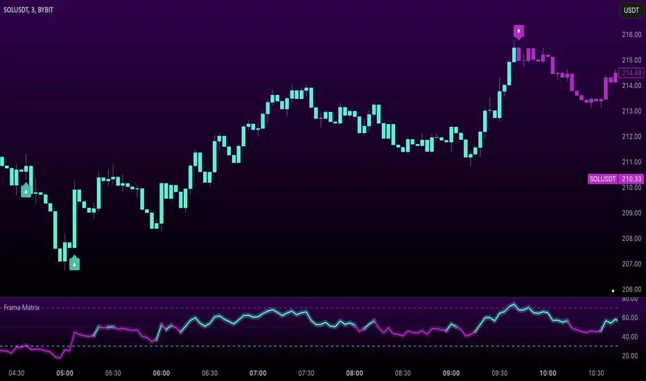
Uptrick: FRAMA Matrix RSIUptrick: FRAMA Matrix RSI
Introduction
The Uptrick: FRAMA Matrix RSI is a momentum-based indicator that integrates the Relative Strength Index (RSI) with the Fractal Adaptive Moving Average (FRAMA). By applying FRAMA's adaptive smoothing to RSI—and further refining it with a Zero-Lag Moving Average (ZLMA)—this script creates a refined and reliable momentum oscillator. The indicator now includes enhanced divergence detection, potential reversal signals, customizable buy/sell signal options, an internal stats table, and a fully customizable bar coloring system for an enhanced visual trading experience.
Why Combine RSI with FRAMA
Traditional RSI is a well-known momentum indicator but has several limitations. It is highly sensitive to price fluctuations, often generating false signals in choppy or volatile markets. FRAMA, in contrast, adapts dynamically to price changes by adjusting its smoothing factor based on market conditions.
By integrating FRAMA into RSI calculations, this indicator reduces noise while preserving RSI's ability to track momentum, adapts to volatility by reducing lag in trending markets and smoothing out choppiness in ranging conditions, enhances trend-following capability for more reliable momentum shifts, and refines overbought and oversold signals by adjusting to the current market structure.
With the new enhancements, such as a manual alpha input, noise filtering, divergence detection, and multiple buy/sell signal options, the indicator offers even greater flexibility and precision for traders. This combination improves the standard RSI by making it more adaptive and responsive to market changes.
Originality
This indicator is unique because it applies FRAMA's adaptive smoothing technique to RSI, creating a dynamic momentum oscillator that adjusts to different market conditions. Many traditional RSI-based indicators either use fixed smoothing methods like exponential moving averages or employ basic RSI calculations without adjusting for volatility.
This script stands out by integrating several elements, including the fractal dimension-based smoothing of FRAMA to reduce noise while retaining responsiveness, the use of Zero-Lag Moving Average smoothing to enhance trend sensitivity and reduce lag, divergence detection to highlight mismatches between price action and RSI momentum, a noise filter and manual alpha option to prevent minor fluctuations from generating false signals, customizable buy/sell signal options that let traders choose between ZLMA-based or FRAMA RSI-based signals, an internal stats table displaying real-time FRAMA calculations such as fractal dimension and the adaptive alpha factor, and a fully customizable bar coloring system to visually distinguish bullish, bearish, and neutral conditions.
Features
Adaptive FRAMA RSI
The indicator applies FRAMA to RSI values, making the momentum oscillator adaptive to volatility while filtering out noise. Unlike a traditional RSI that reacts equally to all price movements, FRAMA RSI adjusts its smoothing factor based on market structure, making it more effective for identifying true momentum shifts.
Zero-Lag Moving Average (ZLMA)
A smoothing technique that minimizes lag while preserving the responsiveness of price movements. It is applied to the FRAMA RSI to further refine signals and ensure smoother trend detection.
Bullish and Bearish Threshold Crossovers
This system compares FRAMA RSI to a user-defined threshold (default is 50). When FRAMA RSI moves above the threshold, it indicates bullish momentum, while movement below signals bearish conditions. The enhanced noise filter ensures that only significant moves trigger signals.
Noise Filter and Manual Alpha
A new noise filter input prevents tiny fluctuations from triggering false signals. In addition, a manual alpha option allows traders to override the automatically computed smoothing factor with a custom value, providing extra control over the indicator’s sensitivity.
Divergence Detection
The indicator identifies divergence patterns by comparing FRAMA RSI pivots to price action. Bullish divergence occurs when price makes a lower low while FRAMA RSI makes a higher low, and bearish divergence occurs when price makes a higher high while FRAMA RSI makes a lower high. These signals can help traders anticipate potential reversals.
Reversal Signals
Labels appear on the chart when FRAMA RSI confirms classic RSI overbought (70) or oversold (30) conditions, providing visual cues for potential trend reversals.
Buy and Sell Signal Options
Traders can now choose between two signal-generation methods. ZLMA-based signals trigger when the ZLMA of FRAMA RSI crosses key overbought (70) or oversold (30) levels, while FRAMA RSI-based signals trigger when FRAMA RSI itself crosses these levels. This added flexibility allows users to tailor the indicator to their preferred trading style.
ZLMA:
FRAMA:
Customizable Alerts
Alerts notify traders when FRAMA RSI crosses key levels, divergence signals occur, reversal conditions are met, or buy/sell signals trigger. This ensures that important trading events are not missed.
Fully Customizable Bar Coloring System
Users can color bars based on different conditions, enhancing visual clarity. Bar coloring modes include: FRAMA RSI threshold (bars change color based on whether FRAMA RSI is above or below the threshold), ZLMA crossover (bars change when ZLMA crosses overbought or oversold levels), buy/sell signals (bars change when official signals trigger), divergence (bars highlight when bullish or bearish divergence is detected), and reversals (bars indicate when RSI reaches overbought or oversold conditions confirmed by FRAMA RSI). The system also remembers the last applied bar color, ensuring a smooth visual transition.
Input Parameters and Features
Core Inputs
RSI Length (default: 14) defines the period for RSI calculations.
FRAMA Lookback (default: 16) determines the length for the FRAMA smoothing function.
RSI Bull Threshold (default: 50) sets the level above which the market is considered bullish and below which it is bearish.
Noise Filter (default: 1.0) ensures that small fluctuations do not trigger false bullish or bearish signals.
Additional Features
Show Bull and Bear Alerts (default: true) enables notifications when FRAMA RSI crosses the threshold.
Enable Divergence Detection (default: false) highlights bullish and bearish divergences based on price and FRAMA RSI pivots.
Show Potential Reversal Signals (default: false) identifies overbought (70) and oversold (30) levels as possible trend reversal points.
Buy and Sell Signal Option (default: ZLMA) allows traders to choose between ZLMA-based signals or FRAMA RSI-based signals for trade entry.
ZLMA Enhancements
ZLMA Length (default: 14) determines the period for the Zero-Lag Moving Average applied to FRAMA RSI.
Visualization Options
Show Internal Stats Table (default: false) displays real-time FRAMA calculations, including fractal dimension and the adaptive alpha smoothing factor.
Show Threshold FRAMA Signals (default: false) plots buy and sell labels when FRAMA RSI crosses the threshold level.
How It Works
FRAMA Calculation
FRAMA dynamically adjusts smoothing based on the price fractal dimension. The alpha smoothing factor is derived from the fractal dimension or can be set manually to maintain responsiveness.
RSI with FRAMA Smoothing
RSI is calculated using the user-defined lookback period. FRAMA is then applied to the RSI to make it more adaptive to volatility. Optionally, ZLMA is applied to further refine the signals and reduce lag.
Bullish and Bearish Threshold Crosses
A bullish condition occurs when FRAMA RSI crosses above the threshold, while a bearish condition occurs when it falls below. The noise filter ensures that only significant trend shifts generate signals.
Buy and Sell Signal Options
Traders can choose between ZLMA crossovers or FRAMA RSI crossovers as the basis for buy and sell signals, offering flexibility in trade entry timing.
Divergence Detection
The indicator identifies divergences where price action and FRAMA RSI momentum do not align, potentially signaling upcoming reversals.
Reversal Signal Labels
When classic RSI overbought or oversold levels are confirmed by FRAMA RSI conditions, reversal labels are added on the chart to highlight potential exhaustion points.
Bar Coloring System
Bars are dynamically colored based on various conditions such as RSI thresholds, ZLMA crossovers, buy/sell signals, divergence, and reversals, allowing traders to quickly interpret market sentiment.
Alerts and Internal Stats
Customizable alerts notify traders of key events, and an optional internal stats table displays real-time calculations (fractal dimension, alpha value, and RSI values) to help users understand the underlying dynamics of the indicator.
Summary
The Uptrick: FRAMA Matrix RSI offers an enhanced approach to momentum analysis by combining RSI with adaptive FRAMA smoothing and additional layers of signal refinement. The indicator now includes adaptive RSI smoothing to reduce noise and improve responsiveness, Zero-Lag Moving Average filtering to minimize lag, divergence and reversal detection to identify potential turning points, customizable buy/sell signal options that let traders choose between different signal methodologies, a fully customizable bar coloring system to visually distinguish market conditions, and an internal stats table for real-time insight into FRAMA calculation parameters.
Whether used for trend confirmation, divergence detection, or momentum-based strategies, this indicator provides a powerful and adaptive approach to trading.
Disclaimer
This script is for informational and educational purposes only. Trading involves risk, and past performance does not guarantee future results. Always conduct proper research and consult with a financial advisor before making trading decisions.
Daily COC Strategy with SHERLOCK WAVESThis indicator implements a unique trading strategy known as the "Daily COC (Candle Over Candle) Strategy" enhanced with "SHERLOCK WAVES" for pattern recognition. It's designed for traders looking to capitalize on specific candlestick formations with a negative risk-reward ratio, with the aim of achieving a high win rate (over 70%) through numerous trading opportunities, despite each trade having a higher risk relative to the reward.
Key Features:
Pattern Recognition: Identifies a setup based on three consecutive candles - a red candle followed by a shooting star, then an entry candle that does not break below the shooting star's low.
Negative Risk/Reward Trade Selection: Focuses on entries where the potential stop loss is greater than the take profit, banking on a high win rate to offset the individual trade's negative risk-reward ratio.
Visual Signals:
Green Label: Marks potential entry points at the high of the candle before the entry.
Green Dot: Indicates a winning trade closure.
Red Dot: Signals a losing trade closure.
Blue Circle: Warns when the current candle is within 2% of breaking above the previous candle's high, suggesting a potential setup is developing.
Green Circle: Plots the take profit level.
Red Circle: Plots the stop loss level.
Dynamic Statistics: A live updating label showing the number of trades, wins, losses, open trades, current account balance, and win percentage.
Customizable Parameters:
Risk % per Trade: Adjust the percentage of your account balance you're willing to risk on each trade.
Initial Account Balance: Set your starting balance for tracking performance.
Start Date for Strategy: Define when the strategy should start calculating from, allowing for backtesting.
Alerts:
An alert condition is set for when a potential trade setup is developing, helping traders prepare for entries.
Usage Tips:
This strategy is predicated on the idea that a high win rate can compensate for the negative risk-reward ratio of individual trades. It might not suit all market conditions or traders' risk profiles.
Use this strategy in conjunction with other analysis methods to validate trade setups.
Note: Always backtest thoroughly before applying to live markets. Consider this tool as part of a broader trading strategy, not a standalone solution. Monitor your win rate and adjust your risk management accordingly to ensure the strategy remains profitable over time.
This description now correctly explains the purpose behind the negative risk-reward ratio in the context of your trading strategy.

Multi-Timeframe RSI Grid Strategy with ArrowsKey Features of the Strategy
Multi-Timeframe RSI Analysis:
The strategy calculates RSI values for three different timeframes:
The current chart's timeframe.
Two higher timeframes (configurable via higher_tf1 and higher_tf2 inputs).
It uses these RSI values to identify overbought (sell) and oversold (buy) conditions.
Grid Trading System:
The strategy uses a grid-based approach to scale into trades. It adds positions at predefined intervals (grid_space) based on the ATR (Average True Range) and a grid multiplication factor (grid_factor).
The grid system allows for pyramiding (adding to positions) up to a maximum number of grid levels (max_grid).
Daily Profit Target:
The strategy has a daily profit target (daily_target). Once the target is reached, it closes all open positions and stops trading for the day.
Drawdown Protection:
If the open drawdown exceeds 2% of the account equity, the strategy closes all positions to limit losses.
Reverse Signals:
If the RSI conditions reverse (e.g., from buy to sell or vice versa), the strategy closes all open positions and resets the grid.
Visualization:
The script plots buy and sell signals as arrows on the chart.
It also plots the RSI values for the current and higher timeframes, along with overbought and oversold levels.
How It Works
Inputs:
The user can configure parameters like RSI length, overbought/oversold levels, higher timeframes, grid spacing, lot size multiplier, maximum grid levels, daily profit target, and ATR length.
RSI Calculation:
The RSI is calculated for the current timeframe and the two higher timeframes using ta.rsi().
Grid System:
The grid system uses the ATR to determine the spacing between grid levels (grid_space).
When the price moves in the desired direction, the strategy adds positions at intervals of grid_space, increasing the lot size by a multiplier (lot_multiplier) for each new grid level.
Entry Conditions:
A buy signal is generated when the RSI is below the oversold level on all three timeframes.
A sell signal is generated when the RSI is above the overbought level on all three timeframes.
Position Management:
The strategy scales into positions using the grid system.
It closes all positions if the daily profit target is reached or if a reverse signal is detected.
Visualization:
Buy and sell signals are plotted as arrows on the chart.
RSI values for all timeframes are plotted, along with overbought and oversold levels.
Example Scenario
Suppose the current RSI is below 30 (oversold), and the RSI on the 60-minute and 240-minute charts is also below 30. This triggers a buy signal.
The strategy enters a long position with a base lot size.
If the price moves against the position by grid_space, the strategy adds another long position with a larger lot size (scaled by lot_multiplier).
This process continues until the maximum grid level (max_grid) is reached or the daily profit target is achieved.
Key Variables
grid_level: Tracks the current grid level (number of positions added).
last_entry_price: Tracks the price of the last entry.
base_size: The base lot size for the initial position.
daily_profit_target: The daily profit target in percentage terms.
target_reached: A flag to indicate whether the daily profit target has been achieved.
Potential Use Cases
This strategy is suitable for traders who want to combine RSI-based signals with a grid trading approach to capitalize on mean-reverting price movements.
It can be used in trending or ranging markets, depending on the RSI settings and grid parameters.
Limitations
The grid trading system can lead to significant drawdowns if the market moves strongly against the initial position.
The strategy relies heavily on RSI, which may produce false signals in strongly trending markets.
The daily profit target may limit potential gains in highly volatile markets.
Customization
You can adjust the input parameters (e.g., RSI length, overbought/oversold levels, grid spacing, lot multiplier) to suit your trading style and market conditions.
You can also modify the drawdown protection threshold or add additional filters (e.g., volume, moving averages) to improve the strategy's performance.
In summary, this script is a sophisticated trading strategy that combines RSI-based signals with a grid trading system to manage entries, exits, and position sizing. It includes features like daily profit targets, drawdown protection, and multi-timeframe analysis to enhance its robustnes

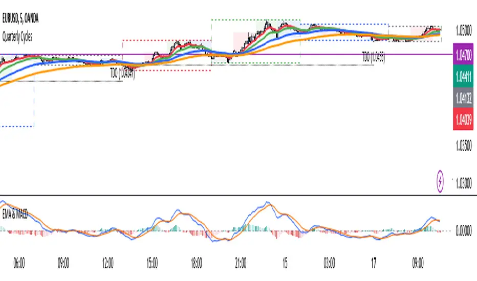
4 EMA & MACDThe indicator that combines Moving Average and MACD into one is very useful for providing a more complete picture of the market. Here's how it works:
Moving Average (MA): This is a trend indicator that smooths the price to show the dominant trend direction. MA helps traders determine whether the market is in an uptrend, downtrend, or sideways. For example, if the price is above the MA, it might indicate an uptrend, while if the price is below the MA, it might indicate a downtrend.
MACD (Moving Average Convergence Divergence): MACD measures market momentum and can provide entry and exit signals based on the difference between two moving averages (fast MA and slow MA). A buy signal occurs when the MACD crosses above the signal line, and a sell signal occurs when the MACD crosses below the signal line.
Combining both gives traders a more complete view:
MA provides an overview of the larger trend direction.
MACD helps identify moments when momentum supports a position for entering or exiting.
Common usage:
Entry: If the price is above the Moving Average (uptrend) and the MACD shows a buy signal (for example, MACD crossing above the signal line), it can be a signal to buy.
Exit: If the price starts moving below the MA and the MACD shows a sell signal, it can be a signal to sell or exit the position.
There is an indicator called MACD + Moving Average Cross, which combines both elements, providing stronger signals and making it easier to follow the market.
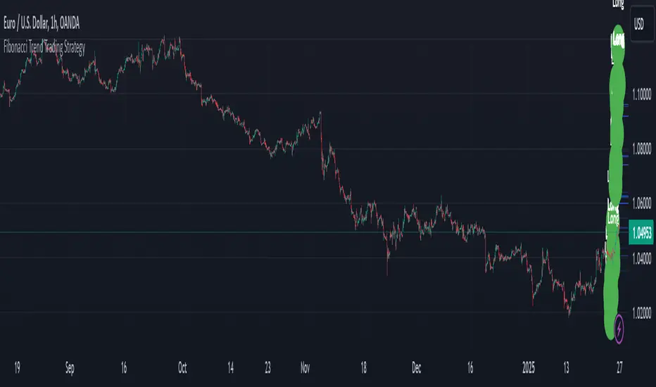
Fibonacci Extension Strt StrategyCore Logic and Steps:
Weekly Trend Identification:
Find the last significant Higher High (HH) and Lower Low (LL) or vice-versa on the Weekly timeframe.
Determine if it's an uptrend (HH followed by LL) or a downtrend (LL followed by HH).
Plot a Fibonacci Extension (or Retracement in reverse order) from the swing point determined to the other significant swing point.
Weekly Retracement Levels:
Display horizontal lines at the 0.236, 0.382, and 0.5 Fibonacci levels from the weekly extension.
Monitor price action on these levels.
Daily Confirmation:
When price hits the Fib levels, examine the Daily chart.
Look for a rejection wick (indicating the pull back is ending) on the identified weekly retracement levels.
Confirm that the price is indeed starting to continue in the direction of the original weekly trend.
Four-Hour Entry:
On the 4H timeframe, plot a new Fib Extension in the opposite direction of the weekly.
If it's an uptrend, the Fib is plotted from last swing low to its swing high. If the weekly trend was bearish the Fib will be plotted from last swing high to the swing low.
Generate an entry when price breaks the high of that candle.
Trade Management:
Entry is on the breakout of the current candle.
Stop Loss: Place the stop loss below the wick of the breakout candle.
Take Profit 1: Close 50% of the position at the 0.5 Fibonacci level. Move the stop loss to breakeven on this position.
Take Profit 2: Close another 25% of the position at the 0.236 Fib level.
Trailing Take Profit: Keep the last 25% open, using a trailing stop loss. (You'll need to define the logic for the trailing stop, e.g., trailing stop using the last high/low)
How to Use in TradingView:
Open a TradingView Chart.
Click on "Pine Editor" at the bottom.
Copy and paste the corrected Pine Script code.
Click "Add to Chart".
The indicator should now be displayed on your chart.
ILD inverse liquidity Divergence StrategyDetermine Bias (Bullish):
H4 chart shows an uptrend with higher highs and higher lows.
Identify a swing high where resting liquidity (buy-side) is likely above.
Look for SMT Divergence (Lower Timeframes):
On M15, EUR/USD makes a higher high while GBP/USD fails to, signaling potential manipulation.
Spot an Inverse Fair Value Gap (IFVG):
Price has impulsively moved up, leaving a fair value gap below.
Wait for a Retracement (Entry):
Price retraces into the IFVG near a Fibonacci 61.8% retracement level.
Enter long here with a SL below the gap.
Set Risk-to-Reward:
SL = 10 pips below the entry.
TP = 20 pips above (1:2 R:R), targeting a resting liquidity zone above a recent swing high.
Monitor and Exit:
Price moves into the liquidity zone, hits TP, and completes the trade.

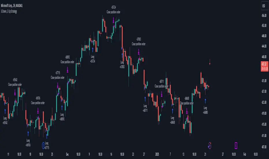
3 Down, 3 Up Strategy█ STRATEGY DESCRIPTION
The "3 Down, 3 Up Strategy" is a mean-reversion strategy designed to capitalize on short-term price reversals. It enters a long position after consecutive bearish closes and exits after consecutive bullish closes. This strategy is NOT optimized and can be used on any timeframes.
█ WHAT ARE CONSECUTIVE DOWN/UP CLOSES?
- Consecutive Down Closes: A sequence of trading bars where each close is lower than the previous close.
- Consecutive Up Closes: A sequence of trading bars where each close is higher than the previous close.
█ SIGNAL GENERATION
1. LONG ENTRY
A Buy Signal is triggered when:
The price closes lower than the previous close for Consecutive Down Closes for Entry (default: 3) consecutive bars.
The signal occurs within the specified time window (between Start Time and End Time).
If enabled, the close price must also be above the 200-period EMA (Exponential Moving Average).
2. EXIT CONDITION
A Sell Signal is generated when the price closes higher than the previous close for Consecutive Up Closes for Exit (default: 3) consecutive bars.
█ ADDITIONAL SETTINGS
Consecutive Down Closes for Entry: Number of consecutive lower closes required to trigger a buy. Default = 3.
Consecutive Up Closes for Exit: Number of consecutive higher closes required to exit. Default = 3.
EMA Filter: Optional 200-period EMA filter to confirm long entries in bullish trends. Default = disabled.
Start Time and End Time: Restrict trading to specific dates (default: 2014-2099).
█ PERFORMANCE OVERVIEW
Designed for volatile markets with frequent short-term reversals.
Performs best when price oscillates between clear support/resistance levels.
The EMA filter improves reliability in trending markets but may reduce trade frequency.
Backtest to optimize consecutive close thresholds and EMA period for specific instruments.
One Shot One Kill ICT [TradingFinder] Liquidity MMXM + CISD OTE🔵 Introduction
The One Shot One Kill trading setup is one of the most advanced methods in the field of Smart Money Concept (SMC) and ICT. Designed with a focus on concepts such as Liquidity Hunt, Discount Market, and Premium Market, this strategy emphasizes precise Price Action analysis and market structure shifts. It enables traders to identify key entry and exit points using a structured Trading Model.
The core process of this setup begins with a Liquidity Hunt. Initially, the price targets areas like the Previous Day High and Previous Day Low to absorb liquidity. Once the Change in State of Delivery(CISD)is broken, the market structure shifts, signaling readiness for trade entry. At this stage, Fibonacci retracement levels are drawn, and the trader enters a position as the price retraces to the 0.618 Fibonacci level.
Part of the Smart Money approach, this setup combines liquidity analysis with technical tools, creating an opportunity for traders to enter high-accuracy trades. By following this setup, traders can identify critical market moves and capitalize on reversal points effectively.
Bullish :
Bearish :
🔵 How to Use
The One Shot One Kill setup is a structured and advanced trading strategy based on Liquidity Hunt, Fibonacci retracement, and market structure shifts (CISD). With a focus on precise Price Action analysis, this setup helps traders identify key market movements and plan optimal trade entries and exits. It operates in two scenarios: Bullish and Bearish, each with distinct steps.
🟣 Bullish One Shot One Kill
In the Bullish scenario, the process starts with the price moving toward the Previous Day Low, where liquidity is absorbed. At this stage, retail sellers are trapped as they enter short trades at lower levels. Following this, the market reverses upward and breaks the CISD, signaling a shift in market structure toward bullishness.
Once this shift is identified, traders draw Fibonacci levels from the lowest point to the highest point of the move. When the price retraces to the 0.618 Fibonacci level, conditions for a buy position are met. The target for this trade is typically the Previous Day High or other significant liquidity zones where major buyers are positioned, offering a high probability of price reversal.
🟣 Bearish One Shot One Kill
In the Bearish scenario, the price initially moves toward the Previous Day High to absorb liquidity. Retail buyers are trapped as they enter long trades near the highs. After the liquidity hunt, the market reverses downward, breaking the CISD, which signals a bearish shift in market structure. Following this confirmation, Fibonacci levels are drawn from the highest point to the lowest point of the move.
When the price retraces to the 0.618 Fibonacci level, a sell position is initiated. The target for this trade is usually the Previous Day Low or other key liquidity zones where major sellers are active.
This setup provides a precise and logical framework for traders to identify market movements and enter trades at critical reversal points.
🔵 Settings
🟣 CISD Logical settings
Bar Back Check : Determining the return of candles to identify the CISD level.
CISD Level Validity : CISD level validity period based on the number of candles.
🟣 LIQUIDITY Logical settings
Swing period : You can set the swing detection period.
Max Swing Back Method : It is in two modes "All" and "Custom". If it is in "All" mode, it will check all swings, and if it is in "Custom" mode, it will check the swings to the extent you determine.
Max Swing Back : You can set the number of swings that will go back for checking.
🟣 CISD Display settings
Displaying or not displaying swings and setting the color of labels and lines.
🟣 LIQUIDITY Display settings
Displaying or not displaying swings and setting the color of labels and lines.
🔵 Conclusion
The One Shot One Kill setup is one of the most effective and well-structured trading strategies for identifying and capitalizing on key market movements. By incorporating concepts such as Liquidity Hunt, CISD, and Fibonacci retracement, this setup allows traders to enter trades with high precision at optimal points.
The strategy emphasizes detailed Price Action analysis and the identification of Smart Money behavior, helping traders to execute successful trades against the general market trend.
With a focus on identifying liquidity in the Previous Day High and Low and aligning it with Fibonacci retracement levels, this setup provides a robust framework for entering both bullish and bearish trades.
The combination of liquidity analysis and Fibonacci retracement at the 0.618 level enables traders to minimize risk and exploit major market moves effectively.
Ultimately, success with the One Shot One Kill setup requires practice, patience, and strict adherence to its rules. By mastering its concepts and focusing on high-probability setups, traders can enhance their decision-making skills and build a sustainable and professional trading approach.

3 Candle AlertThis is a test for integration using a webhook. I am publishing it so I can share it. Ultimately, this is what we want to do:
1. Trade Entry Rules:
Wait until at least the 3rd bar of the day (15 minutes after market open) before entering the first trade.
Order of Priority for Entry:
Look for two consecutive volume bars of the same color (the second bar must have higher volume than the first).
Look for a “price push” beyond the high or low of the day (as determined in the first 15 minutes).
2. Trading Direction:
If the volume bars are RED, I take a Long Position.
If the volume bars are GREEN, I take a Short Position.
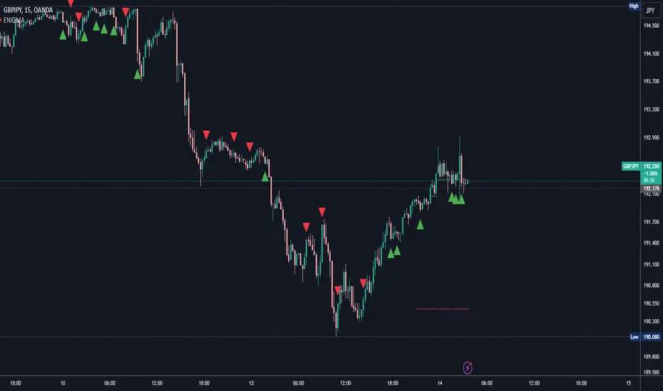
ENIGMA Signals with Retests Select higher Time FrameENIGMA Signals with Retests – Script Description
The "ENIGMA Signals with Retests" script is a unique indicator designed for traders who prefer precision trading based on price action retests of key levels derived from higher timeframes. This tool is ideal for those employing multi-timeframe analysis strategies, helping them detect high-probability trade entries when the price interacts with significant support and resistance levels.
What Does This Script Do?
This indicator identifies key levels from a higher timeframe selected by the user (e.g., 4-hour or daily), then tracks price action on lower timeframes to provide actionable buy and sell signals when the price retests these levels. It visually plots the key levels on the chart and triggers alerts for potential trade opportunities when conditions are met.
How It Works
Key Level Detection:
The script uses custom functions to detect recent swing highs and swing lows on the selected higher timeframe (such as 4H or Daily). These levels represent potential areas of support and resistance where price reactions are likely to occur.
Multi-Timeframe Analysis:
The indicator leverages the request.security() function to retrieve price data from the user-defined higher timeframe and plots horizontal lines on the chart for the most recent swing highs and lows.
Retest-Based Signals:
Once the key levels are plotted, the script continuously monitors the price on the lower timeframe:
A Buy Signal is triggered when the price closes below a key high level and then moves back above it, indicating a potential bullish retest.
A Sell Signal is triggered when the price closes above a key low level and then moves back below it, indicating a potential bearish retest.
These retest signals are displayed as green and red arrows on the chart, helping traders identify optimal entry points.
Alerts for Retests:
The script includes built-in alert conditions that notify traders when a valid retest signal occurs. This allows traders to react promptly without constantly monitoring the chart.
How to Use the Script
Select Your Key Timeframe:
From the input settings, choose a higher timeframe that suits your trading style (e.g., 4H for intraday trading or Daily for swing trading).
Adjust Visual Preferences:
Customize the line style (solid, dashed, or dotted) and length of the plotted levels.
Toggle labels for the levels on or off as per your preference.
Trade Execution:
Once a retest signal appears on the lower timeframe, consider entering a trade in the direction of the signal. The buy signal suggests a potential long entry, while the sell signal indicates a potential short entry.
Set Alerts:
Use the alert conditions provided to get notified whenever a valid retest occurs. This helps in reducing screen time and improving trading efficiency.
Underlying Concepts
This script is grounded in the principles of support and resistance, retests, and breakout trading. By focusing on multi-timeframe key levels, it aligns with widely used trading concepts like:
Breakout and Retest: Entering trades after a confirmed breakout and successful retest of a significant level.
Swing Highs and Lows: Recognizing swing points to identify strong price reaction zones.
Multi-Timeframe Confluence: Enhancing trade probability by ensuring that the signals on lower timeframes correspond with key levels from higher timeframes.
Why This Script Is Unique
Unlike many generic trend-following or scalping indicators, "ENIGMA Signals with Retests" offers:
Precision Signals: It only provides signals when specific retest conditions are met, reducing false signals and noise.
Multi-Timeframe Customization: Users can tailor the higher timeframe to their strategy, making it versatile for various trading styles.
Alert Functionality: Alerts are integrated, allowing traders to stay updated without constantly monitoring the charts.
This script is perfect for traders looking for a systematic way to trade retests of key levels across multiple timeframes. Whether you're a scalper, day trader, or swing trader, "ENIGMA Signals with Retests" can help improve your precision and timing in the market.
4H CRT (1AM and 5AM)This TradingView script is designed to assist traders in implementing the "4-Hour Candle Ranges Theory Strategy (CRT)" by identifying key levels and setups based on the 1am and 4am (5am) 4-hour candles. This strategy is particularly effective for trading high-volatility assets such as Gold, EUR/USD, NAS100, US30, and S&P500, with US30 showing a notably high win rate. Here's how the strategy works:
Key Features:
1. Marking 1am and 4am 4-Hour Candle Ranges
- The script highlights the high and low of the 1am 4-hour candle.
- It visually tracks whether the high or low of the 1am candle is taken out by the subsequent 4-hour candle (5am).
2. Entry Setup Rules
- Primary Setup: Wait for the high or low of the 1am candle to be taken out by the 5am candle. Once this sweep occurs, wait for a Market Structure Shift (MSS) on the lower time frame (15min) to confirm your entry.
- Secondary Setup: If the 5am candle fails to take out the high or low of the 1am candle, the setup focuses on the levels formed by the 5am candle.
3. Trade Execution on 15-Minute Timeframe
- The script supports a lower time frame (15min) view to identify MSS and fine-tune entries.
4. Rinse and Repeat
- This process can be applied daily for consistent opportunities across the specified assets.
Advantages:
- Provides clear visual markers for key levels based on the 4-hour candles.
- Automates level plotting, saving traders time and reducing manual errors.
- Integrates well with the 15-minute timeframe for precise entry triggers.
- Optimized for popular trading instruments, especially US30 for a higher probability of success.
This script simplifies the application of CRT by automating the process of identifying and marking critical levels, enabling traders to focus on executing high-probability setups effectively.
Created by Hamid (poraymanfx)

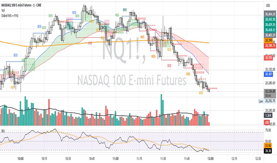
Dabel MS + FVGThis script is designed to assist traders by identifying market structures, imbalances, and potential trade opportunities using Break of Structure (BOS) and Market Structure Shifts (MSS). It visually highlights imbalances in price action, key pivots, and market structure changes, providing actionable information for making trading decisions.
Key features:
Imbalances Detection: Highlights bullish and bearish price gaps (Fair Value Gaps) using colored boxes. Users can choose the line style (solid, dashed, or dotted) for imbalance midlines.
Market Structure Analysis: Tracks pivot highs and lows to identify BOS and MSS in two separate market structures with adjustable pivot strengths.
Customizable Visualization: Allows users to choose line styles, colors, and display options for both imbalances and market structures.
Alerts: Alerts traders when BOS or MSS occur, helping to monitor the market effectively.
Trading Strategy
Imbalance Trading:
Imbalances (gaps) represent areas where supply or demand was left unfilled. These gaps often act as magnet zones where the price revisits to fill.
Bullish Imbalance: Look for buying opportunities when price enters a green imbalance zone.
Bearish Imbalance: Look for selling opportunities when price enters a red imbalance zone.
Use the midline of the imbalance box as a key reference point for potential reversals.
Break of Structure (BOS) and Market Structure Shift (MSS):
BOS: Indicates a continuation of the existing trend. For example:
Bullish BOS: Look for continuation in the uptrend after a high is broken.
Bearish BOS: Look for continuation in the downtrend after a low is broken.
MSS: Suggests a potential reversal in market structure. For example:
Bullish MSS: Indicates a possible shift from a bearish to bullish market.
Bearish MSS: Indicates a potential shift from a bullish to bearish market.
Multiple Market Structures:
This script provide two sets of market structures, allowing traders to compare short-term and long-term trends.
Adjust the pivot strength to suit your trading style (lower for intraday trading, higher for swing or positional trading).
Entry and Exit:
Entry: Look for entries near imbalances or after confirmed BOS/MSS in line with the overall trend.
Exit: Place stop-loss below/above recent pivots and take profit at nearby support/resistance or imbalance zones.
For New Traders
Focus on Basics: Understand what BOS and MSS mean and how they signal trend direction or reversals.
Use Alerts: Rely on the script's alert system to catch important moments without staring at charts all day.
Start Small: Test this strategy on a demo account before using it live. You can understand it more with practice.
Adaptive Momentum Reversion StrategyThe Adaptive Momentum Reversion Strategy: An Empirical Approach to Market Behavior
The Adaptive Momentum Reversion Strategy seeks to capitalize on market price dynamics by combining concepts from momentum and mean reversion theories. This hybrid approach leverages a Rate of Change (ROC) indicator along with Bollinger Bands to identify overbought and oversold conditions, triggering trades based on the crossing of specific thresholds. The strategy aims to detect momentum shifts and exploit price reversions to their mean.
Theoretical Framework
Momentum and Mean Reversion: Momentum trading assumes that assets with a recent history of strong performance will continue in that direction, while mean reversion suggests that assets tend to return to their historical average over time (Fama & French, 1988; Poterba & Summers, 1988). This strategy incorporates elements of both, looking for periods when momentum is either overextended (and likely to revert) or when the asset’s price is temporarily underpriced relative to its historical trend.
Rate of Change (ROC): The ROC is a straightforward momentum indicator that measures the percentage change in price over a specified period (Wilder, 1978). The strategy calculates the ROC over a 2-period window, making it responsive to short-term price changes. By using ROC, the strategy aims to detect price acceleration and deceleration.
Bollinger Bands: Bollinger Bands are used to identify volatility and potential price extremes, often signaling overbought or oversold conditions. The bands consist of a moving average and two standard deviation bounds that adjust dynamically with price volatility (Bollinger, 2002).
The strategy employs two sets of Bollinger Bands: one for short-term volatility (lower band) and another for longer-term trends (upper band), with different lengths and standard deviation multipliers.
Strategy Construction
Indicator Inputs:
ROC Period: The rate of change is computed over a 2-period window, which provides sensitivity to short-term price fluctuations.
Bollinger Bands:
Lower Band: Calculated with a 18-period length and a standard deviation of 1.7.
Upper Band: Calculated with a 21-period length and a standard deviation of 2.1.
Calculations:
ROC Calculation: The ROC is computed by comparing the current close price to the close price from rocPeriod days ago, expressing it as a percentage.
Bollinger Bands: The strategy calculates both upper and lower Bollinger Bands around the ROC, using a simple moving average as the central basis. The lower Bollinger Band is used as a reference for identifying potential long entry points when the ROC crosses above it, while the upper Bollinger Band serves as a reference for exits, when the ROC crosses below it.
Trading Conditions:
Long Entry: A long position is initiated when the ROC crosses above the lower Bollinger Band, signaling a potential shift from a period of low momentum to an increase in price movement.
Exit Condition: A position is closed when the ROC crosses under the upper Bollinger Band, or when the ROC drops below the lower band again, indicating a reversal or weakening of momentum.
Visual Indicators:
ROC Plot: The ROC is plotted as a line to visualize the momentum direction.
Bollinger Bands: The upper and lower bands, along with their basis (simple moving averages), are plotted to delineate the expected range for the ROC.
Background Color: To enhance decision-making, the strategy colors the background when extreme conditions are detected—green for oversold (ROC below the lower band) and red for overbought (ROC above the upper band), indicating potential reversal zones.
Strategy Performance Considerations
The use of Bollinger Bands in this strategy provides an adaptive framework that adjusts to changing market volatility. When volatility increases, the bands widen, allowing for larger price movements, while during quieter periods, the bands contract, reducing trade signals. This adaptiveness is critical in maintaining strategy effectiveness across different market conditions.
The strategy’s pyramiding setting is disabled (pyramiding=0), ensuring that only one position is taken at a time, which is a conservative risk management approach. Additionally, the strategy includes transaction costs and slippage parameters to account for real-world trading conditions.
Empirical Evidence and Relevance
The combination of momentum and mean reversion has been widely studied and shown to provide profitable opportunities under certain market conditions. Studies such as Jegadeesh and Titman (1993) confirm that momentum strategies tend to work well in trending markets, while mean reversion strategies have been effective during periods of high volatility or after sharp price movements (De Bondt & Thaler, 1985). By integrating both strategies into one system, the Adaptive Momentum Reversion Strategy may be able to capitalize on both trending and reverting market behavior.
Furthermore, research by Chan (1996) on momentum-based trading systems demonstrates that adaptive strategies, which adjust to changes in market volatility, often outperform static strategies, providing a compelling rationale for the use of Bollinger Bands in this context.
Conclusion
The Adaptive Momentum Reversion Strategy provides a robust framework for trading based on the dual concepts of momentum and mean reversion. By using ROC in combination with Bollinger Bands, the strategy is capable of identifying overbought and oversold conditions while adapting to changing market conditions. The use of adaptive indicators ensures that the strategy remains flexible and can perform across different market environments, potentially offering a competitive edge for traders who seek to balance risk and reward in their trading approaches.
References
Bollinger, J. (2002). Bollinger on Bollinger Bands. McGraw-Hill Professional.
Chan, L. K. C. (1996). Momentum, Mean Reversion, and the Cross-Section of Stock Returns. Journal of Finance, 51(5), 1681-1713.
De Bondt, W. F., & Thaler, R. H. (1985). Does the Stock Market Overreact? Journal of Finance, 40(3), 793-805.
Fama, E. F., & French, K. R. (1988). Permanent and Temporary Components of Stock Prices. Journal of Political Economy, 96(2), 246-273.
Jegadeesh, N., & Titman, S. (1993). Returns to Buying Winners and Selling Losers: Implications for Stock Market Efficiency. Journal of Finance, 48(1), 65-91.
Poterba, J. M., & Summers, L. H. (1988). Mean Reversion in Stock Prices: Evidence and Implications. Journal of Financial Economics, 22(1), 27-59.
Wilder, J. W. (1978). New Concepts in Technical Trading Systems. Trend Research.