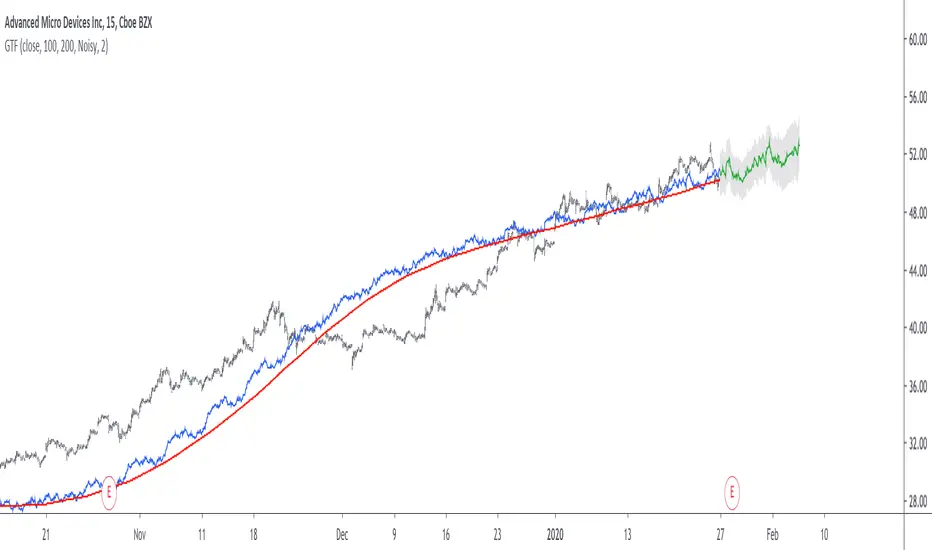
Grand Trend Forecasting - A Simple And Original Approach Today we'll link time series forecasting with signal processing in order to provide an original and funny trend forecasting method, the post share lot of information, if you just want to see how to use the indicator then go to the section "Using The Indicator".
Time series forecasting is an area dealing with the prediction of future values of a series by using a specific model, the model is the main tool that is used for forecasting, and is often an expression based on a set of predictor terms and parameters, for example the linear regression (model) is a 1st order polynomial (expression) using 2 parameters and a predictor variable ax + b . Today we won't be using the linear regression nor the LSMA.
In time series analysis we can describe the time series with a model, in the case of the closing price a simple model could be as follows :
Price = Trend + Cycles + Noise
The variables of the model are the components, such model is additive since we add the component with each others, we should be familiar with each components of the model, the trend represent a simple long term variation of high amplitude, the cycles are periodic fluctuations centered around 0 of varying period and amplitude, the noise component represent shorter term irregular variations with mean 0.
As a trader we are mostly interested by the cycles and the trend, altho the cycles are relatively more technical to trade and can constitute parasitic fluctuations (think about retracements in a trend affecting your trend indicator, causing potential false signals).
If you are curious, in signal processing combining components has a specific name, "synthesis" , here we are dealing with additive synthesis, other type of synthesis are more specific to audio processing and are relatively more complex, but could be used in technical analysis.
So what to do with our components ? If we want to trade the trend, we should estimate right ? Estimating the trend component involve removing the cycle and noise component from the price, if you have read stuff about filters you should know where i'am going, yep, we should use filters, in the case of keeping the trend we can use a simple moving average of relatively high period, and here we go.
However the lag problem, which is recurrent, come back again, we end up with information easier to interpret (here the trend, which is a simple fluctuation such as a line or other smooth curve) at the cost of decision timing, that is unfortunate but as i said the information, here the moving average output, is relatively simple, and could be easily forecasted right ? If you plot a moving average of high period it would be easier for you to forecast its future values. And thats what we aim to do today, provide an estimate of the trend that should be easy to forecast, and should fit to the price relatively well in order to produce forecast that could determine the position of future closing prices observations.
Estimating And Forecasting The Trend
The parameter of the indicator dealing with the estimation of the trend is length , with higher values of length attenuating the cycle and noise component in the price, note however that high values of length can return a really long term trend unlike a simple moving average, so a small value of length, 14 for example can still produce relatively correct estimate of trend.
here length = 14.
The rough estimate of the trend is t in the code, and is an IIR filter, that is, it is based on recursion. Now i'll pass on the filter design explanation but in short, weights are constants, with higher weights allocated to the previous length values of the filter, you can see on the code that the first part of t is similar to an exponential moving average with :
t(n) = 0.9t(n-length) + 0.1*Price
However while the EMA only use the precedent value for the recursion, here we use the precedent length value, this would just output a noisy and really slow output, therefore in order to create a better fit we add : 0.9*(t(n-length) - t(n-2length)) , and this create the rough trend estimate that you can see in blue. On the parameters, 0.9 is used since it gives the best estimate in my opinion, higher values would create more periodic output and lower values would just create a rougher output.
The blue line still contain a residual of the cycle/noise component, this is why it is smoothed with a simple moving average of period length. If you are curious, a filter estimating the trend but still containing noisy fluctuations is called "Notch" filter, such filter would depending on the cutoff remove/attenuate mid term cyclic fluctuations while preserving the trend and the noise, its the opposite of a bandpass filter.
In order to forecast values, we simply sum our trend estimate with the trend estimate change with period equal to the forecasting horizon period, this is a really really simple forecasting method, but it can produce decent results, it can also allows the forecast to start from the last point of the trend estimate.
Using The Indicator
We explained the length parameter in the precedent section, src is the input series which the trend is estimated, forecast determine the forecasting horizon, recommend values for forecast should be equal to length, length/2 or length*2, altho i strongly recommend length.
here length and forecast are both equal to 14 .
The corrective parameter affect the trend estimate, it reduce the overshoot and can led to a curve that might fit better to the price.
The indicator with the non corrective version above, and the corrective one below.
The source parameter determine the source of the forecast, when "Noisy" is selected the source is the blue line, and produce a noisy forecast, when "Smooth" is selected the source is the moving average of t , this create a smoother forecast.
The width interval control...the width of the intervals, they can be seen above and under the forecast plot, they are constructed by adding/subtracting the forecast with the forecast moving average absolute error with respect to the price. Prediction intervals are often associated with a probability (determining the probability of future values being between the interval) here we can't determine such probability with accuracy, this require (i think) an analysis of the forecasting distribution as well as assumptions on the distribution of the forecasting error.
Finally it is possible to see historical forecasts, that is, forecasts previously generated by checking the "Show Historical Forecasts" option.
Examples
Good forecasts mostly occur when the price is close to the trend estimate, this include the following highlighted periods on AMD 15TF with default settings :
We can see the same thing at the end of EURUSD :
However we can't always obtain suitable fits, here it is isn't sufficient on BTCUSD :
We can see wide intervals, we could change length or use the corrective option to get better results, another option is to use a log scale.
We will end the examples with the log SPX, who posses a linear trend, so for example a linear model such as a linear regression would be really adapted, lets see how the indicator perform :
Not a great fit, we could try to use an higher length value and use "Smooth" :
Most recent fits are quite decent.
Conclusions
A forecasting indicator has been presented in this post. The indicator use an original approach toward estimating the trend component in the closing price. Of course i should have given statistics related to the forecasting error, however such analysis is worth doing with better methods and in more advanced environment allowing for optimization.
But we have learned some stuff related to signal processing as well as time series analysis, seeing a time series as the sum of various components is really helpful when it comes to make sense of chaotic and noisy series and is a basic topic in time series analysis.
You can see that in this new year i work harder on the visual of my indicators without trying to fall in the label addict trap, something that i wasn't really doing before, let me know what do you think of it.
Thanks for reading !
"curve" için komut dosyalarını ara
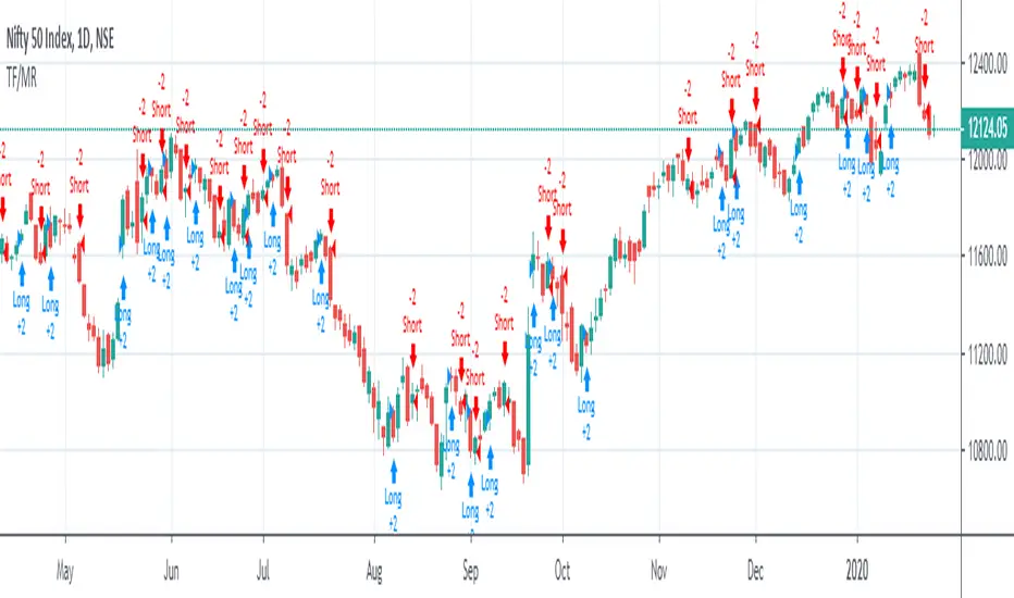
Trend Following or Mean RevertingThe strategy checks nature of the instruments. It Buys if the close is greater than yesterday's high, reverse the position if the close is lower than yesterday's low and repeat the process.
1. If it is trend following then the equity curve will be in uptrend
2. If it is mean reverting then the equity curve will be downtrend
Thanks to Rayner Teo.
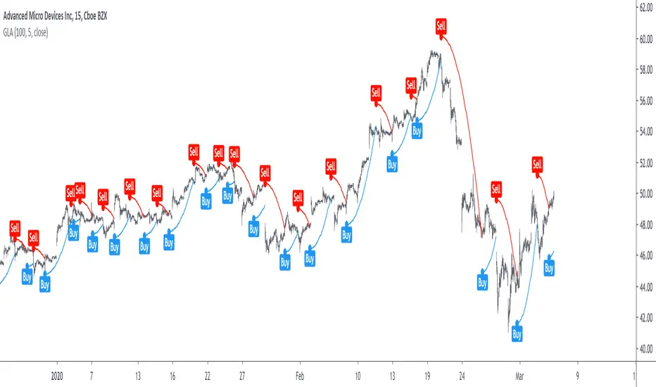
Grover Llorens Activator [alexgrover & Lucía Llorens] Trailing stops play a key role in technical analysis and are extremely popular trend following indicators. Their main strength lie in their ability to minimize whipsaws while conserving a decent reactivity, the most popular ones include the Supertrend, Parabolic SAR and Gann Hilo activator. However, and like many indicators, most trailing stops assume an infinitely long trend, which penalize their ability to provide early exit points, this isn't the case of the parabolic SAR who take this into account and thus converge toward the price at an increasing speed the longer a trend last.
Today a similar indicator is proposed. From an original idea of alexgrover & Lucía Llorens who wanted to revisit the classic parabolic SAR indicator, the Llorens activator aim to converge toward the price the longer a trend persist, thus allowing for potential early and accurate exit points. The code make use of the idea behind the price curve channel that you can find here :
I tried to make the code as concise as possible.
The Indicator
The indicator posses 2 user settings, length and mult , length control the rate of convergence of the indicator, with higher values of length making the indicator output converge more slowly toward the price. Mult is also related with the rate of convergence, basically once the price cross the trailing stop its value will become equal to the previous trailing stop value plus/minus mult*atr depending on the previous trailing stop value, therefore higher values of mult will require more time for the trailing stop to reach the closing price, use higher values of mult if you want to avoid potential whipsaws.
Above the indicator with slow convergence time (high length) and low mult.
Points with early exit points are highlighted.
Usage For Oscillators
The difference between the closing price and an overlay indicator can provide an oscillator with characteristics depending on the indicators used for differencing, Lucía Llorens stated that we should find indicators for differencing that highlight the cycles in the price, in other terms : Price - Signal , where we want to find Signal such that we maximize the visibility of the cycles, it can be demonstrated that in the case where the closing price is an additive model : Trend + Cycles + Noise , the zero lag estimation of the Trend component can allow for the conservation of the cycle and noise component, that is : Price - Estimate(Trend) , for example the difference between the price and moving average isn't optimal because of the moving average lag, instead the use of zero lag moving averages is more suitable, however the proposed indicator allow for a surprisingly good representation of the cycles when using differencing.
The normalization of this oscillator (via the RSI) allow to make the peak amplitude of the cycles more constant. Note however that such method can return an output with a sign inverse to the one of the original cycle component.
Conclusion
We proposed an indicator which share the logic of the SAR indicator, that is using convergence toward the price in order to provide early exit points detection. We have seen that this indicator can be used to highlight cycles when used for differencing and i don't exclude publishing more indicators based on this method.
Lucía Llorens has been a great person to work with, and provided enormous feedback and support while i was coding the indicator, this is why i include her in the indicator name as well as copyright notice. I hope we can make more indicators togethers in the future.
(altho i was against using buy/sells labels xD !)
Thanks for reading !
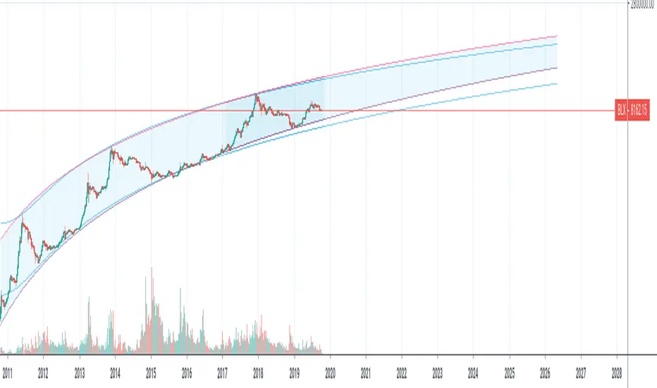
Yope BTC PL channelThis is a new version of the old "Yope BTC tops channel", but modified to reflect a power-law curve fitted, similar to the model proposed by Harold Christopher Burger in his medium article "Bitcoin’s natural long-term power-law corridor of growth".
My original tops channel fitting is still there for comparison. In fact, it looks like the old tops channel was a bit too pessimistic.
Note that these channels are still pure naive curve-fitting, and do not represent an underlying model that explains it, like is the case for PlanB's "Modeling Bitcoin's Value with Scarcity" which uses Stock-to-Flow.
The motivation for this exercise is to observe how long this empirical extrapolation is valid. Will the price of bitcoin stay in either of both channels?
Note on usage: This script _only_ works with the BLX "BraveNewCoin Liquid Index for Bitcoin" in the 1D, 3D and 1W time-frames!
It may be necessary to zoom in and out a few times to overcome drawing glitches caused by the extreme time-shifting of plots in order to draw the extrapolated part.
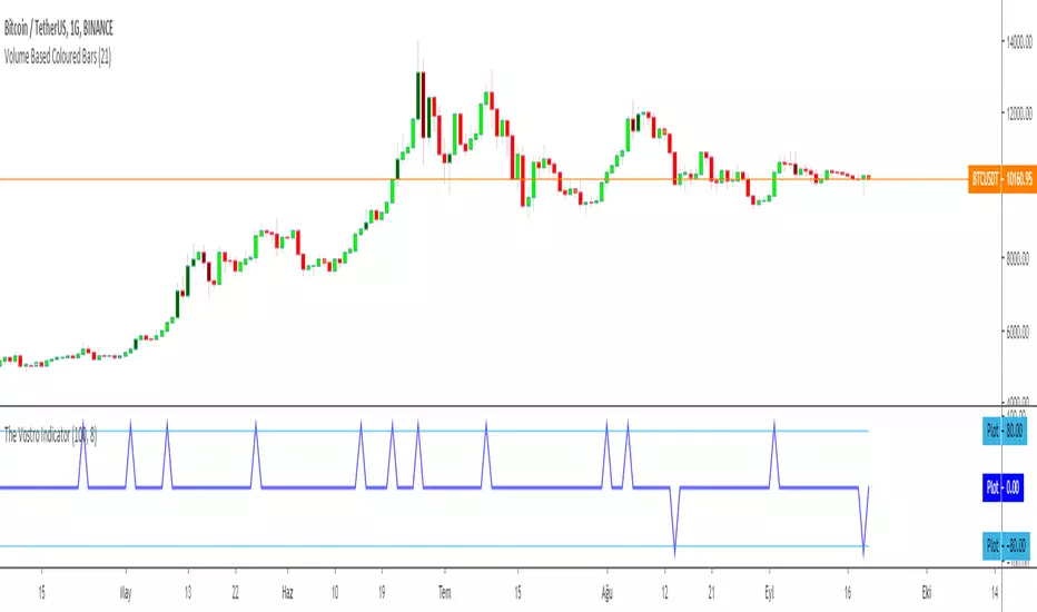
The Vostro Indicator by KIVANÇ fr3762The VOSTRO indicator is a trend indicator that automatically provides buying and selling signals. The indicator marks in a window the potential turning points. The indicator is recommended for scalping.
The Vostro indicator determines the overbought zones (value greater than +80) and the oversold zones (less than the -80 level)
BUY signal: The Vostro curve moves below the -80 level and forms a trough – Turnaround of the upward trend
SELL signal: The Vostro curve moves above the +80 level and forms a peak – Downward trend
further info:
www.prorealcode.com
Here's the link to a complete list of all my indicators:
t.co
Yazar: KıvanÇ @fr3762 twitter
Şimdiye kadar paylaştığım indikatörlerin tam listesi için: t.co
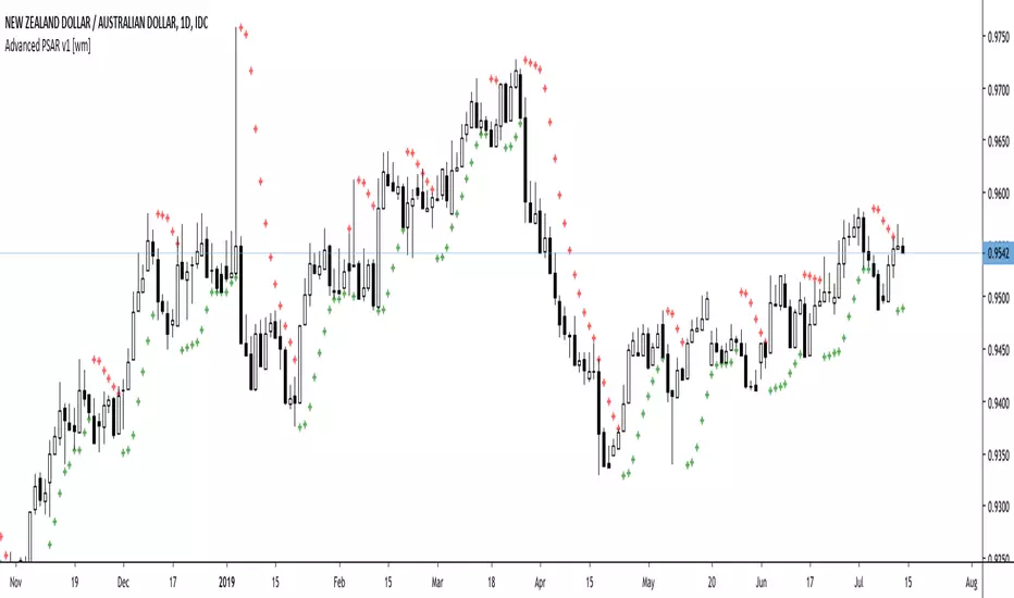
Advanced PSAR v1 [wm]A port off Dennis Meyers Advance PSAR outlined in Stocks and Commodities V13:4
The shape, slope and speed of the SAR is controlled by three parameters: the starting acceleration factor (AF), the increment that the AF can change when a new price high or low is made, and the maximum AF. Because of the way the SAR is calculated, the shape of the SAR curve resembles a parabola - hence its name.
Most software packages only allow the user to vary the AF increment and the AF maximum, fixing the starting AF at 0.02. This restriction hampers the trend-following abilities of the parabolic.
Frequently as the SAR hugs the price curve, it is penetrated by a price bar by a minuscule amount, causing the SAR to generate an opposite signal. The price then immediately turns around and resumes going in the direction it was going before this penetration occurred, causing a costly whipsaw loss.
Many of the whipsaw losses are caused by noise or randomness in the price series. Thus, if the SAR is to represent the trend of a real price series, it must have the capability to ignore penetrations of noise level amounts. To this end, I have modified the parabolic SAR formula to include a variable that allows the SAR not to reverse unless penetrated by a defined amount. This new parameter is defined as ‘XO Increment’ for crossover increment
This version is configured for pips. If using on other assets with much larger values should be used. Also note the starting values have not been optimised. Should users of this script find good values please comment and share with the community if you could
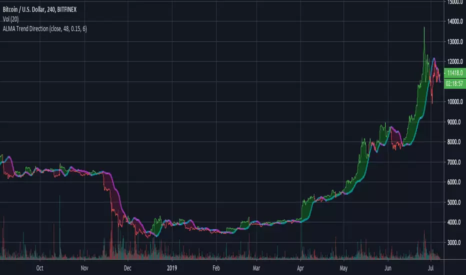
ALMA Trend DirectionHere is a very simple tool that uses the Arnaud Legoux Moving Average(ALMA). The ALMA is based on a normal distribution and is a reliable moving average due to its ability to reduce lag while still keeping a high degree of smoothness.
Input Options:
-Offset : Value in range {0,1} that adjusts the curve of the Gaussian Distribution. A higher value will result in higher responsiveness but lower smoothness. A lower value will mean higher smoothness but less responsiveness.
-Length : The lookback window for the ALMA calculation.
-Sigma : Defines the sharpe of the curve coefficients.
I find that this indicator is best used with a longer length and a 4 Hour timeframe. Overall, its purpose is to help identify the direction of a trend and determine whether a security is in an uptrend or a downtrend. For this purpose, it is best to use a lower offset value since we are looking to identify long-term, significant price movement rather than small fluctuations.
The Chart:
The ALMA is plotted as the aqua and pink alternating line. It is aqua when bullish and pink when bearish.
The low price for each candle is then compared to the ALMA. If the low is greater than the ALMA, then there is a bullish trend and the area between the candles and ALMA is filled green. The area between the ALMA and candles is filled red when the low price is less than the ALMA.
The difference between the slow ALMA and candles can reveal a lot about the current market state. If there is a significant green gap between the two, then we know that there is a significant uptrend taking place. On the other hand, a large red gap would indicate a significant downtrend. Similarly, if the gap between the two is narrowing and the ALMA line switches from aqua to pink, then we know that a reversal could be coming shortly.
~Happy Trading~
Double ALMAIncludes fast and slow Arnaud Legoux Moving Averages (ALMA). ALMA is a moving average based on a Gaussian(normal) distribution that reduces lag while still retaining smoothness.
Input Options:
-Offset : Value in range {0,1} that adjusts the curve of the Gaussian Distribution. A higher value will result in higher responsiveness but lower smoothness. A lower value will mean higher smoothness but less responsiveness.
-Lengths : The lookback for each ALMA calculation.
-Sigma : Defines the sharpe of the curve coefficients.
The slow ALMA is the thickest red and green alternating line that indicates bullish or bearish movement. When slow ALMA is bullish, the graph's background changes to green. When the slow ALMA is bearish, the background is red.
The fast ALMA uses a smaller lookback and is more responsive than the slow ALMA as a result of the shorter length and higher default offset parameter.
The two dotted lines represent (slowALMA +/- 1.25 * stdev(slowALMA, slowALMA period *2)).
The indicator bases its buy and sell signals based on the trend identified by the slow ALMA and the fast ALMA's crossings of the standard deviation bands.
Comes with pre-set buy and sell alerts.

Modified Gann HiLo ActivatorIntroduction
The gann hilo activator is a trend indicator developed by Robert Krausz published into W. D. Gann Treasure Discovered: Simple Trading Plans for Stocks & Commodities . This indicator crate a trailing stop aiming to show the direction of the trend.
This indicator is fairly easy to compute and dont require lot of skills to understand. First we calculate the simple moving average of both price high and price low, when the close price is higher than the moving average of the price high the indicator return the moving average of the price low, else the indicator return the moving average of the price high if the close price is lower than the moving average of the price low.
My indicator add a different calculation method in order to avoid whipsaw trades as well as adding significance to the moving average length. A Median method has been added to provide more robustness.
The Indicator
The indicator is a simple trailing stop aiming to show the direction of the trend. The indicator use a different source instead of the price high/low for its calculation. The first method is the "SMA" method which like the classic hilo indicator use a simple moving average for the calculation of the indicator.
Sma Method with length = 25
The "Median" use a moving median instead of a simple moving average, this provide more robustness.
Median Method with length = 25
The shape is less curved and the indicator can sometimes avoid whipsaw with high's length periods.
Mult Parameter
The mult parameter is a parameter set to be lower or equal to 1 and greater or equal to 0. High values allow the indicator to be far from the price thus avoiding whipsaw trades, lower ones lower the distance from the price. A mult parameter of 0.1 approximate the original hilo indicator.
In blue the indicator with mult = 0.1 and in radical red the original hilo activator.
Conclusion
The modifications allow more control over the indicator as well as adding more robustness while the original one is destined to fail when market price is more complex.
Thanks for reading :)
For any questions/suggestions feel free to pm me

Quadratic Regression Slope [DW]This is a study geared toward identifying price trends using Quadratic regression.
Quadratic regression is the process of finding the equation of a parabola that best fits the set of data being analyzed.
In this study, first a quadratic regression curve is calculated, then the slope of the curve is calculated and plotted.
Custom bar colors are included. The color scheme is based on whether the slope is positive or negative, and whether it is increasing or decreasing.

XPloRR MA-Trailing-Stop StrategyXPloRR MA-Trailing-Stop Strategy
Long term MA-Trailing-Stop strategy with Adjustable Signal Strength to beat Buy&Hold strategy
None of the strategies that I tested can beat the long term Buy&Hold strategy. That's the reason why I wrote this strategy.
Purpose: beat Buy&Hold strategy with around 10 trades. 100% capitalize sold trade into new trade.
My buy strategy is triggered by the fast buy EMA (blue) crossing over the slow buy SMA curve (orange) and the fast buy EMA has a certain up strength.
My sell strategy is triggered by either one of these conditions:
the EMA(6) of the close value is crossing under the trailing stop value (green) or
the fast sell EMA (navy) is crossing under the slow sell SMA curve (red) and the fast sell EMA has a certain down strength.
The trailing stop value (green) is set to a multiple of the ATR(15) value.
ATR(15) is the SMA(15) value of the difference between the high and low values.
The scripts shows a lot of graphical information:
The close value is shown in light-green. When the close value is lower then the buy value, the close value is shown in light-red. This way it is possible to evaluate the virtual losses during the trade.
the trailing stop value is shown in dark-green. When the sell value is lower then the buy value, the last color of the trade will be red (best viewed when zoomed)(in the example, there are 2 trades that end in gain and 2 in loss (red line at end))
the EMA and SMA values for both buy and sell signals are shown as a line
the buy and sell(close) signals are labeled in blue
How to use this strategy?
Every stock has it's own "DNA", so first thing to do is tune the right parameters to get the best strategy values voor EMA , SMA, Strength for both buy and sell and the Trailing Stop (#ATR).
Look in the strategy tester overview to optimize the values Percent Profitable and Net Profit (using the strategy settings icon, you can increase/decrease the parameters)
Then keep using these parameters for future buy/sell signals only for that particular stock.
Do the same for other stocks.
Important : optimizing these parameters is no guarantee for future winning trades!
Here are the parameters:
Fast EMA Buy: buy trigger when Fast EMA Buy crosses over the Slow SMA Buy value (use values between 10-20)
Slow SMA Buy: buy trigger when Fast EMA Buy crosses over the Slow SMA Buy value (use values between 30-100)
Minimum Buy Strength: minimum upward trend value of the Fast SMA Buy value (directional coefficient)(use values between 0-120)
Fast EMA Sell: sell trigger when Fast EMA Sell crosses under the Slow SMA Sell value (use values between 10-20)
Slow SMA Sell: sell trigger when Fast EMA Sell crosses under the Slow SMA Sell value (use values between 30-100)
Minimum Sell Strength: minimum downward trend value of the Fast SMA Sell value (directional coefficient)(use values between 0-120)
Trailing Stop (#ATR): the trailing stop value as a multiple of the ATR(15) value (use values between 2-20)
Example parameters for different stocks (Start capital: 1000, Order=100% of equity, Period 1/1/2005 to now) compared to the Buy&Hold Strategy(=do nothing):
BEKB(Bekaert): EMA-Buy=12, SMA-Buy=44, Strength-Buy=65, EMA-Sell=12, SMA-Sell=55, Strength-Sell=120, Stop#ATR=20
NetProfit: 996%, #Trades: 6, %Profitable: 83%, Buy&HoldProfit: 78%
BAR(Barco): EMA-Buy=16, SMA-Buy=80, Strength-Buy=44, EMA-Sell=12, SMA-Sell=45, Strength-Sell=82, Stop#ATR=9
NetProfit: 385%, #Trades: 7, %Profitable: 71%, Buy&HoldProfit: 55%
AAPL(Apple): EMA-Buy=12, SMA-Buy=45, Strength-Buy=40, EMA-Sell=19, SMA-Sell=45, Strength-Sell=106, Stop#ATR=8
NetProfit: 6900%, #Trades: 7, %Profitable: 71%, Buy&HoldProfit: 2938%
TNET(Telenet): EMA-Buy=12, SMA-Buy=45, Strength-Buy=27, EMA-Sell=19, SMA-Sell=45, Strength-Sell=70, Stop#ATR=14
NetProfit: 129%, #Trade

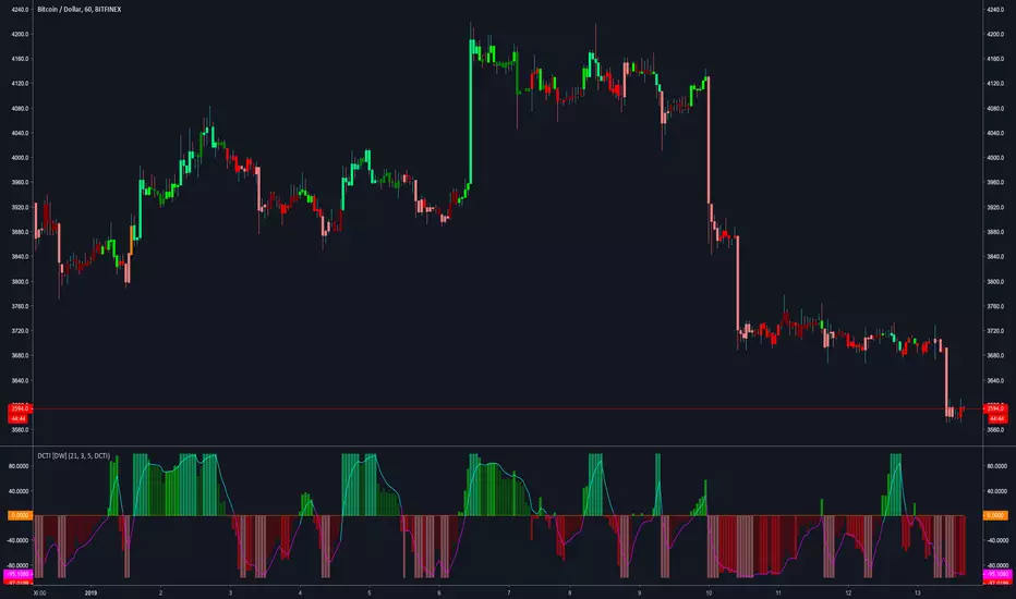
Donchian Channel Trend Intensity [DW]This is an experimental study designed to analyze trend intensity using two Donchian Channels.
The DCTI curve is calculated by comparing the differences between Donchian highs and lows over a major an minor period, and expressing them as a positive and negative percentage.
The curve is then smoothed with an exponential moving average to provide a signal line.
Custom bar colors included with two coloring methods to choose from.
AWESOME OSCILLATOR V2 by KIVANCfr3762AWESOME OSCILLATOR V2 by KIVANC @fr3762
CONVERTING THE OSCILLATOR to a curved line and added a 7 period SMA as a signal line,
crosses are BUY or SELL signals like in MACD
Buy: when AO line crosses above signal line
Sell: when Signal line crosses above AO line
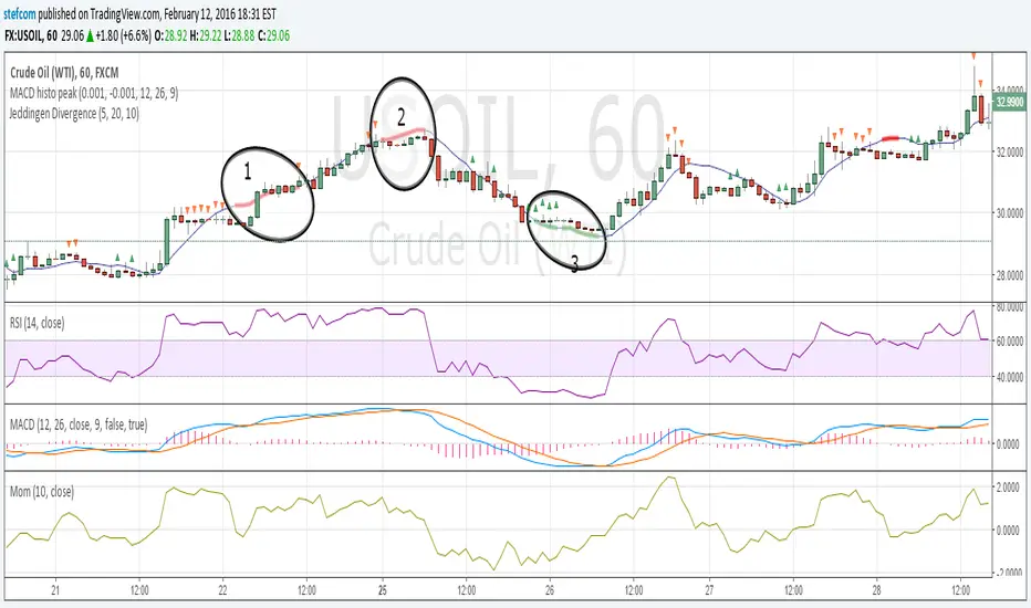
Stefan Krecher: Jeddingen DivergenceThe main idea is to identify a divergence between momentum and price movement. E.g. if the momentum is rising but price is going down - this is what we call a divergence. The divergence will be calculated by comparing the direction of the linear regression curve of the price with the linear regression curve of momentum.
A bearish divergence can be identified by a thick red line, a bullish divergence by a green line.
When there is a divergence, it is likeley that the current trend will change it's direction.
Looking at the chart, there are three divergences that need to get interpreted:
1) bearish divergence, RSI is overbought but MACD does not clearly indicate a trend change. Right after the divergence, price and momentum are going up. No clear signal for a sell trade
2) bearish divergence, RSI still overbought, MACD histogram peaked, MACD crossed the signal line, price and momentum are going down. Very clear constellation for a sell trade.
3) two bullish diverences, RSI is oversold, MACD crossover near the end of the second divergence, price and momentum started rising. Good constellation for a buy trade. Could act as exit signal for the beforementioned sell trade.
More information on the Jeddingen Divergence is available here: www.forexpython.com
Power Law Correlation Indicator 2.0 The Power Law Correlation Indicator is an attempt to chart when a stock/currency/futures contract goes parabolic forming a upward or downward curve that accelerates according to power laws.
I've read about power laws from Sornette Diedler ( www.marketcalls.in ). And I think the theory is a good one.
The idea behind this indicator is that it will rise to 1.0 as the curve resembles a parabolic up or down swing. When it is below zero, the stock will flatten out.
There are many ways to use this indicator. One way I am testing it out is in trading Strangles or Straddle option trades. When this indicator goes below zero and starts to turn around, it means that it has flattened out. This is like a squeeze indicator. (see the TTM squeeze indicator).
Since this indicator goes below zero and the squeeze plays tend to be mean-reverting; then its a great time to put on a straddle/strangle.
Another way to use it is to think of it in terms of trend strength. Think of it as a kind of ADX, that measures the trend strength. When it is rising, the trend is strong; when it is dropping, the trend is weak.
Lastly I think this indicator needs some work. I tried to put the power (x^n) function into it but my coding skill is limited. I am hoping that Lazy Bear or Ricardo Santos can do it some justice.
Also I think that if we can figure out how to do other power law graphs, perhaps we can plot them together on one indicator.
So far I really like this one for finding Strangle spots. So check it out.
Peace
SpreadEagle71

Stabilized HMA ScalperStabilized HMA Scalper / Stab. HMA 2.0
Stabilized HMA Scalper is a visual trend-structure overlay indicator designed to highlight directional momentum, trend alignment, and market state through a combination of adaptive moving averages and contextual visual cues.
The indicator blends a Hull Moving Average (HMA) for responsiveness with an ALMA-based baseline filter to stabilize trend interpretation and reduce noise. The result is a clean, visually expressive framework for reading market structure directly on the price chart.
Core Design Philosophy
This script is built around trend confirmation and state visualization, not prediction or automation.
All elements are calculated on confirmed bar closes and do not repaint.
The indicator focuses on three analytical dimensions:
1. Dual Moving Average Structure
Hull Moving Average (HMA)
Acts as the primary momentum curve.
Designed for fast reaction to directional changes.
Slope behavior is used to infer momentum expansion or contraction.
ALMA Baseline Filter
Provides a stabilizing reference for broader trend context.
Helps distinguish directional movement from short-term fluctuations.
Used as a structural filter rather than a trigger mechanism.
2. Trend State Visualization
When HMA slope and price position relative to the ALMA baseline align, the indicator visually highlights the active market state:
Bullish alignment: upward momentum with supportive structure
Bearish alignment: downward momentum with confirming structure
Neutral / range: mixed conditions or transitional phases
A dynamic gradient fill between HMA and ALMA visually reinforces this alignment, offering an immediate understanding of trend strength and continuity.
3. Visual Markers & Labels
Discrete chart markers may appear at moments when momentum structure transitions into a new aligned state.
These markers are contextual annotations, intended to draw attention to changes in trend conditions rather than to provide standalone decisions.
They are based solely on historical price data and are fully non-repainting.
Dashboard
An optional on-chart dashboard summarizes the current market state classification (Bullish / Bearish / Range) based on the internal trend logic.
Position and size are fully configurable.
Designed for at-a-glance situational awareness.
Reflects the same logic used in the chart visuals.
Usage Disclaimer
This indicator is provided for technical analysis and educational purposes only.
It does not generate financial advice or guarantee outcomes and should be used as part of a broader analytical workflow.

Macro 6-PackMacro 6-Pack dashboard: SPX momentum, VIX, HY credit spread, 10Y yield shifts, DXY trend, and 2s10s curve.

[CT] D&W PPO + RBF + DivergenceThis indicator combines two separate ideas into one tool so you can read trend context from your price chart while timing momentum shifts from a clean oscillator panel. The first component is the Daily and Weekly Percentage Price Oscillator (D&W PPO), which measures the relationship between two EMA spreads that are intentionally built to reflect two “speeds” of market structure. The “weekly” leg is calculated as the percentage distance between a slower and faster EMA pair (L1 and L2), and the “daily” leg is calculated as the percentage distance between a shorter EMA pair (L3 and L4), but both are normalized by the same long EMA (e2) so the values behave like a percent-based oscillator rather than raw points. The script then combines those two legs by creating R = W + D, and it plots the histogram as R − W, which simplifies to D. That is not a mistake, it is the point of the design. By setting the baseline at “R equals W,” the zero line becomes a very intuitive threshold that tells you whether the shorter-term push is adding to the longer-term bias or subtracting from it. When the histogram is above zero, the daily component is supportive of the larger trend pressure, and when it is below zero, the daily component is opposing it. The histogram color is intentionally binary and stable, green when the histogram is at or above zero and red when it is below, so the panel reads like a momentum confirmation tool rather than a noisy oscillator that constantly shifts shades.
The second component is the RBF Price Trail, which is drawn on the upper price chart even though the indicator itself lives in a lower panel. This line is not a moving average in the traditional sense. It is a Radial Basis Function kernel smoother that weights recent prices based on their similarity rather than only their recency. In plain terms, the kernel attempts to build a smoother “baseline” that adapts to the shape of price action, and then the script optionally wraps that baseline inside an ATR band and applies a Supertrend-like trailing clamp. When the ATR band is enabled, the line will not simply track the kernel value, it will trail price and hold its position until price forces it to ratchet. This behavior is what makes it useful as a structure-aligned trend line rather than just another smoothing curve. When the adaptive band boost is enabled, the band width is multiplied by a factor that grows when recent price change is large relative to a lookback normalization window. That means the trailing mechanism can adapt to fast markets by changing the effective band behavior, which helps reduce whipsaws in choppy conditions while still allowing the line to respond when volatility expands. The line color is determined by where price closes relative to the trail, bullish when price is above the trail and bearish when price is below it, and you can optionally color your actual chart candles from either the PPO state or the RBF state depending on what you want your eyes to follow.
The settings are organized so you can control each module without changing how the core PPO trend logic behaves. The PPO settings L1, L2, L3, and L4 define the EMA lengths used to compute the weekly leg W and the daily leg D. Increasing these values makes the oscillator slower and smoother, while decreasing them makes it react faster to recent movement. “Show W line” is simply a visual aid, it plots the W line in the oscillator panel so you can see the longer-term component, but it does not change the histogram logic. “Histogram thickness” is purely visual and controls how thick the column bars are. The PPO colors are the two base colors used for the histogram state, green when the daily component is supportive and red when it is opposing.
The RBF settings control what you see on the upper chart. “Show RBF on Price Chart” turns the trail line on or off. “Source” chooses which price series feeds the kernel, and close is usually the cleanest choice. “Kernel Length” determines how many bars the kernel uses; a larger value makes the baseline smoother and slower, and a smaller value makes it more reactive. “Gamma Adj” controls how quickly the kernel’s weights decay as price becomes dissimilar, so higher gamma tends to make the kernel react more sharply to changes while lower gamma produces a broader smoothing effect. “Use ATR Trail Band” is the switch that turns the kernel baseline into a trailing band line, and it is the reason the line can “hold” and then ratchet instead of moving continuously like a normal moving average. “ATR Length” and “ATR Factor” control the width of that band, and widening the band will generally reduce flips and noise at the cost of later signals. “Use Adaptive Band Boost” turns on the volatility normalization idea, “Boost Normalization Lookback” defines how far back the script looks to determine what counts as a large price change, and “Boost Multiplier” controls how strongly the band behavior is adjusted during those periods. The line width and bull/bear colors are visual controls only.
Price bar coloring is intentionally handled with a single selector so you do not end up with two modules fighting to color candles differently. If you choose “Off,” nothing on the main chart is recolored. If you choose “PPO,” your price candles reflect whether the PPO histogram is above or below zero. If you choose “RBF,” your price candles reflect whether price is above or below the RBF trail. Most traders will pick one and stick with it so the chart communicates a single bias at a glance.
The divergence module is optional and is designed to be a confirmation layer rather than a primary trigger. When enabled, it can mark regular divergence and hidden divergence, and it lets you decide what the pivots should be based on. The divergence source can be the PPO histogram or the R line, depending on whether you want divergence measured on the cleaner momentum component or on the combined series. “Key off pivots” determines whether pivot detection is driven by oscillator pivots or by price pivots. If you choose oscillator pivots, divergence anchors are found where the oscillator makes pivot highs or lows and those are compared against price at the same points. If you choose price pivots, the pivots are taken from price first and the oscillator value at those pivot bars is used for the comparison, which can feel more intuitive when you want divergence to respect obvious swing structure on the chart. Pivot Left and Pivot Right control how strict the swing definition is, larger values create fewer but more meaningful pivots and smaller values create more frequent signals. “Mark on Price Chart” adds tiny markers on the candles at the pivot location so you can see where the divergence event was confirmed, while the oscillator panel uses lines and labels to make the divergence relationship obvious.
For trading, the cleanest way to use this tool is to separate “bias” from “timing.” The RBF Price Trail is your bias filter because it is structure-like and tends to hold and ratchet rather than constantly drifting. When price is closing above the trail and the trail is colored bullish, you treat the market as long-biased and you focus on long setups, pullbacks, and continuation entries. When price is closing below the trail and the trail is bearish, you treat the market as short-biased and you focus on short setups, rallies, and continuation shorts. The PPO histogram is then your timing and pressure confirmation. In an up-bias, the highest quality continuation conditions are when the histogram is above zero and stays above zero through pullbacks, because that means the shorter-term pressure is still supporting the longer-term drift. When the histogram dips below zero during an up-bias, it is a warning that the daily component is now opposing, which often corresponds to a deeper pullback, a rotation, or a period of consolidation, so you either wait for the histogram to recover above zero or you tighten expectations and manage risk more aggressively. In a down-bias, the mirror logic applies: the best continuation conditions are when the histogram is below zero, and pushes above zero tend to represent countertrend rotations or pauses inside the bearish condition.
Divergence is best used as an early warning and a location filter, not as a standalone entry button. Regular bullish divergence, where price makes a lower low but the oscillator makes a higher low, can signal bearish pressure is weakening and is most useful when it appears while price is below the RBF trail but failing to continue downward, because it often precedes a reclaim of the trail or at least a meaningful rotation. Regular bearish divergence, where price makes a higher high but the oscillator makes a lower high, can signal bullish pressure is weakening and is most useful when it appears while price is above the trail but extension is failing, because it often precedes a drop back to the trail or a full flip. Hidden divergence is a continuation concept. Hidden bullish divergence, where price makes a higher low while the oscillator makes a lower low, often shows up during pullbacks in an uptrend and can help you confirm continuation as long as the RBF bias remains bullish. Hidden bearish divergence, where price makes a lower high while the oscillator makes a higher high, often shows up during rallies in a downtrend and can help you confirm continuation as long as the RBF bias remains bearish. In practice, you’ll get the best results when you only act on divergence that aligns with the RBF bias for hidden divergence continuation, and you treat regular divergence as a caution or reversal setup only when it occurs near a meaningful swing and is followed by a bias change or a strong momentum shift on the PPO.
The most practical workflow is to keep the RBF trail visible on the price chart as your regime guide, keep the PPO histogram as your momentum confirmation, and decide in advance whether you want candle coloring to represent the PPO state or the RBF state so your eyes are not reading two different meanings at once. if you want the cleanest “trend-following” behavior, color candles by the RBF trail and use the PPO histogram as the timing trigger. If you want the cleanest “momentum-first” behavior, color candles by PPO and treat the RBF trail as the higher-level filter for whether you should press a move or fade it.

Strategy Battle: Lump Sum vs. DCA vs. Dip BuyingSummary This indicator is a "Strategy Battle" simulator designed to answer the ultimate investing question: Is it better to invest immediately, Dollar Cost Average (DCA), or wait for a market crash?
Unlike standard back-testers, this script simulates a realistic "High-Yield Savings" environment. It acknowledges that cash sitting on the sidelines is not dead money—it earns interest (e.g., 3-5%) while waiting for a buying opportunity. This levels the playing field and allows for a fair comparison between being fully invested vs. keeping "dry powder" for a crash.
The script compares 4 distinct strategies simultaneously on your chart, starting with a fresh yearly budget every January 1st.
he 4 Strategies
🔵 Option 1: Lump Sum (The "Set & Forget")
Takes the entire yearly budget and invests it all on the first trading day of the year.
Pros: Maximizes "time in the market."
Cons: vulnerable to buying at immediate peaks.
🟠 Option 2: DCA (The "Steady Earner")
Splits the yearly budget into 12 equal parts.
Invests monthly regardless of price.
The "Fairness" Twist: The money waiting to be spent sits in the cash pile and accumulates interest until it is deployed.
🟢 Option 3: Regression Sniper (The "Math Hunter")
Keeps the entire budget in cash (earning interest).
Watches a dynamic Linear Regression Channel.
Trigger: If the price drops below the channel, it goes "All-In," deploying all accumulated cash and interest immediately to buy the dip.
🔴 Option 4: Manual Sniper (The "Trend Hunter")
Keeps the entire budget in cash (earning interest).
Watches a User-Defined Growth Line (e.g., a straight line growing at 10% per year).
Trigger: If the price drops below this specific valuation line, it goes "All-In."
Detailed Settings & Options
💰 Money Settings
Yearly Budget ($): The amount of fresh capital injected into the simulation every January 1st.
Cash Interest Rate (%): The annual interest rate earned on uninvested cash (compounded monthly). This is crucial for accurately simulating the "opportunity cost" of holding cash.
⚙️ Sniper Settings (Option 3)
Channel Baseline Length: How far back the math looks to determine the "fair value" curve.
Vertical Shift (%): Move the buy zone up or down. Negative numbers (e.g., -5) make the strategy more conservative, waiting for deeper crashes.
Source: Defaults to Low to catch market wicks and intraday crashes.
📈 Manual Line Settings (Option 4)
Start Price ($): The valuation of the asset at the start of the simulation (Jan 1, Start Year).
Yearly Growth (%): The expected "fair" growth rate of the asset (e.g., S&P 500 average is ~10%).
Vertical Shift (%): Slide the manual line up or down to fine-tune your buy signal.
👁️ Visual Settings
Show Buy Price: Displays the exact dollar amount invested and the stock price at the moment of the buy on the chart labels.
Show Lump Sum Markers: Adds a Blue label at the start of every year to visualize the Lump Sum entry.
Show DCA Markers: Adds small Orange labels for every monthly buy.

VWAP-Anchored MACD [BOSWaves]VWAP-Anchored MACD - Volume-Weighted Momentum Mapping With Zero-Line Filtering
Overview
The VWAP-Anchored MACD delivers a refined momentum model built on volume-weighted price rather than raw closes, giving you a more grounded view of trend strength during sessions, weeks, or months.
Instead of tracking two EMAs of price like a standard MACD, this tool reconstructs the MACD engine using anchored VWAP as the core input. The result is a momentum structure that reacts to real liquidity flow, filters out weak crossovers near the zero line, and visualizes acceleration shifts with clear, high-contrast gradients.
This indicator acts as a precise momentum map that adapts in real time. You see how weighted price is accelerating, where valid crossovers form, and when trend conviction is strong enough to justify execution.
It uses gradient line coloring to show bullish or bearish momentum, histogram shading to highlight energy shifts, cross dots to mark valid crossovers, optional buy/sell diamonds for execution cues, and candle coloring to display trend strength at a glance.
Theoretical Foundation
Traditional MACD compares the difference between two exponential moving averages of price.
This variant replaces price with anchored VWAP, making the calculation sensitive to actual traded volume across your chosen period (Session, Week, or Month).
Three principles drive the logic:
Anchored VWAP Momentum : Price is weighted by volume and aggregated across the selected anchor. The fast and slow VWAP-EMAs then expose how liquidity-corrected momentum is expanding or contracting.
Zero-Line Distance Filtering : Crossover signals that occur too close to the zero line are removed. This eliminates the common MACD problem of generating weak, directionless signals in choppy phases.
Directional Visualization : MACD line, signal line, histogram, candle colors, and optional diamond markers all react to shifts in VWAP-momentum, giving you a clean structural read on market pressure.
Anchoring VWAP to session, weekly, or monthly resets creates a systematic framework for tracking how capital flow is driving momentum throughout each trading cycle.
How It Works
The core engine processes momentum through several mapped layers:
VWAP Aggregation : Price × volume is accumulated until the anchor resets. This creates a continuous, liquidity-corrected VWAP curve.
MACD Construction : Fast and slow VWAP-EMAs define the MACD line, while a smoothed signal line identifies edges where momentum shifts.
Zero-Line Distance Filter : MACD and signal must both exceed a threshold distance from zero for a crossover to count as valid. This prevents fake crossovers during compression.
Visual Momentum Layers : It uses gradient line coloring to show bullish or bearish momentum, histogram shading to highlight energy shifts, cross dots to mark valid crossovers, optional buy/sell diamonds for execution cues, and candle coloring to display trend strength at a glance.
This layered structure ensures you always know whether momentum is strengthening, fading, or transitioning.
Interpretation
You get a clean, structural understanding of VWAP-based momentum:
Bullish Phases : MACD > Signal, histogram expands, candles turn bullish, and crossovers occur above the threshold.
Bearish Phases : MACD < Signal, histogram drives lower, candles shift bearish, and downward crossovers trigger below the threshold.
Neutral/Compression : Both lines remain near the zero boundary, histogram flattens, and signals are suppressed to avoid noise.
This creates a more disciplined version of MACD momentum reading - less noise, more conviction, and better alignment with liquidity.
Strategy Integration
Trend Continuation : Use VWAP-MACD crossovers that occur far from the zero line as higher-conviction entries.
Zero-Line Rejection : Watch for histogram contractions near zero to anticipate flattening momentum and potential reversal setups.
Session/Week/Month Anchors : Session anchor works best for intraday flows. Weekly or monthly anchor structures create cleaner macro momentum reads for swing trading.
Signal-Only Execution : Optional buy/sell diamonds give you direct points to trigger trades without overanalyzing the chart.
This indicator slots cleanly into any momentum-following system and offers higher signal quality than classic MACD variants due to the volume-weighted core.
Technical Implementation Details
VWAP Reset Logic : Session (D), Week (W), or Month (M)
Dynamic Fast/Slow VWAP EMAs : Fully configurable lengths, smoothing and anchor settings
MACD/Signal Line Framework : Traditional structure with volume-anchored input
Zero-Line Filtering : Adjustable threshold for structural confirmation
Dual Visualization Layers : MACD body + histogram + crosses + candle coloring
Optimized Performance : Lightweight, fast rendering across all timeframes
Optimal Application Parameters
Timeframes:
1- 15 min : Short-term momentum scalping and rapid trend shifts
30- 240 min : Balanced momentum mapping with clear structural filtering
Daily : Macro VWAP regime identification
Suggested Configuration:
Fast Length : 12
Slow Length : 26
Signal Length : 9
Zero Threshold : 200 - 500 depending on asset range
These suggested parameters should be used as a baseline; their effectiveness depends on the asset volatility, liquidity, and preferred entry frequency, so fine-tuning is expected for optimal performance.
Performance Characteristics
High Effectiveness:
Assets with strong intraday or session-based volume cycles
Markets where volume-weighted momentum leads price swings
Trend environments with strong acceleration
Reduced Effectiveness:
Ultra-choppy markets hugging the VWAP axis
Sessions with abnormally low volume
Ranges where MACD naturally compresses
Disclaimer
The VWAP-Anchored MACD is a structural momentum tool designed to enhance directional clarity - not a guaranteed predictor. Performance depends on market regime, volatility, and disciplined execution. Use it alongside broader trend, volume, and structural analysis for optimal results.

Impulse Reactor RSI-SMA Trend Indicator [ApexLegion]Impulse Reactor RSI-SMA Trend Indicator
Introduction and Theoretical Background
Design Rationale
Standard indicators frequently generate binary 'BUY' or 'SELL' signals without accounting for the broader market context. This often results in erratic "Flip-Flop" behavior, where signals are triggered indiscriminately regardless of the prevailing volatility regime.
Impulse Reactor was engineered to address this limitation by unifying two critical requirements: Quantitative Rigor and Execution Flexibility.
The Solution
Composite Analytical Framework This script is not a simple visual overlay of existing indicators. It is an algorithmic synthesis designed to function as a unified decision-making engine. The primary objective was to implement rigorous quantitative analysis (Volatility Normalization, Structural Filtering) directly within an alert-enabled framework. This architecture is designed to process signals through strict, multi-factor validation protocols before generating real-time notifications, allowing users to focus on structurally validated setups without manual monitoring.
How It Works
This is not a simple visual mashup. It utilizes a cross-validation algorithm where the Trend Structure acts as a gatekeeper for Momentum signals:
Logic over Lag: Unlike simple moving average crossovers, this script uses a 15-layer Gradient Ribbon to detect "Laminar Flow." If the ribbon is knotted (Compression), the system mathematically suppresses all signals.
Volatility Normalization: The core calculation adapts to ATR (Average True Range). This means the indicator automatically expands in volatile markets and contracts in quiet ones, maintaining accuracy without constant manual tweaking.
Adaptive Signal Thresholding: It incorporates an 'Anti-Greed' algorithm (Dynamic Thresholding) that automatically adjusts entry criteria based on trend duration. This logic aims to mitigate the risk of entering positions during periods of statistical trend exhaustion.
Why Use It?
Market State Decoding: The gradient Ribbon visualizes the underlying trend phase in real-time.
◦ Cyan/Blue Flow: Strong Bullish Trend (Laminar Flow).
◦ Magenta/Pink Flow: Strong Bearish Trend.
◦ Compressed/Knotted: When the ribbon lines are tightly squeezed or overlapping, it signals Consolidation. The system filters signals here to avoid chop.
Noise Reduction: The goal is not to catch every pivot, but to isolate high-confidence setups. The logic explicitly filters out minor fluctuations to help maintain position alignment with the broader trend.
⚖️ Chapter 1: System Architecture
Introduction: Composite Analytical Framework
System Overview
Impulse Reactor serves as a comprehensive technical analysis engine designed to synthesize three distinct market dimensions—Momentum, Volatility, and Trend Structure—into a unified decision-making framework. Unlike traditional methods that analyze these metrics in isolation, this system functions as a central processing unit that integrates disparate data streams to construct a coherent model of market behavior.
Operational Objective
The primary objective is to transition from single-dimensional signal generation to a multi-factor assessment model. By fusing data from the Impulse Core (Volatility), Gradient Oscillator (Momentum), and Structural Baseline (Trend), the system aims to filter out stochastic noise and identify high-probability trade setups grounded in quantitative confluence.
Market Microstructure Analysis: Limitations of Conventional Models
Extensive backtesting and quantitative analysis have identified three critical inefficiencies in standard oscillator-based strategies:
• Bounded Oscillator Limitations (The "Oscillation Trap"): Traditional indicators such as RSI or Stochastics are mathematically constrained between fixed values (0 to 100). In strong trending environments, these metrics often saturate in "overbought" or "oversold" zones. Consequently, traders relying on static thresholds frequently exit structurally valid positions prematurely or initiate counter-trend trades against prevailing momentum, resulting in suboptimal performance.
• Quantitative Blindness to Quality: Standard moving averages and trend indicators often fail to distinguish the qualitative nature of price movement. They treat low-volume drift and high-velocity expansion identically. This inability to account for "Volatility Quality" leads to delayed responsiveness during critical market events.
• Fractal Dissonance (Timeframe Disconnect): Financial markets exhibit fractal characteristics where trends on lower timeframes may contradict higher timeframe structures. Manual integration of multi-timeframe analysis increases cognitive load and susceptibility to human error, often resulting in conflicting biases at the point of execution.
Core Design Principles
To mitigate the aforementioned systemic inefficiencies, Impulse Reactor employs a modular architecture governed by three foundational principles:
Principle A:
Volatility Precursor Analysis Market mechanics demonstrate that volatility expansion often functions as a leading indicator for directional price movement. The system is engineered to detect "Volatility Deviation" — specifically, the divergence between short-term and long-term volatility baselines—prior to its manifestation in price action. This allows for entry timing aligned with the expansion phase of market volatility.
Principle B:
Momentum Density Visualization The system replaces singular momentum lines with a "Momentum Density" model utilizing a 15-layer Simple Moving Average (SMA) Ribbon.
• Concept: This visualization represents the aggregate strength and consistency of the trend.
• Application: A fully aligned and expanded ribbon indicates a robust trend structure ("Laminar Flow") capable of withstanding minor counter-trend noise, whereas a compressed ribbon signals consolidation or structural weakness.
Principle C:
Adaptive Confluence Protocols Signal validity is strictly governed by a multi-dimensional confluence logic. The system suppresses signal generation unless there is synchronized confirmation across all three analytical vectors:
1. Volatility: Confirmed expansion via the Impulse Core.
2. Momentum: Directional alignment via the Hybrid Oscillator.
3. Structure: Trend validation via the Baseline. This strict filtering mechanism significantly reduces false positives in non-trending (choppy) environments while maintaining sensitivity to genuine breakouts.
🔍 Chapter 2: Core Modules & Algorithmic Logic
Module A: Impulse Core (Normalized Volatility Deviation)
Operational Logic The Impulse Core functions as a volatility-normalized momentum gauge rather than a standard oscillator. It is designed to identify "Volatility Contraction" (Squeeze) and "Volatility Expansion" phases by quantifying the divergence between short-term and long-term volatility states.
Volatility Z-Score Normalization
The formula implements a custom normalization algorithm. Unlike standard oscillators that rely on absolute price changes, this logic calculates the Z-Score of the Volatility Spread.
◦ Numerator: (atr_f - atr_s) captures the raw momentum of volatility expansion.
◦ Denominator: (std_f + 1e-6) standardizes this value against historical variance.
◦ Result: This allows the indicator scales consistently across assets (e.g., Bitcoin vs. Euro) without manual recalibration.
f_impulse() =>
atr_f = ta.atr(fastLen) // Fast Volatility Baseline
atr_s = ta.atr(slowLen) // Slow Volatility Baseline
std_f = ta.stdev(atr_f, devLen) // Volatility Standard Deviation
(atr_f - atr_s) / (std_f + 1e-6) // Normalized Differential Calculation
Algorithmic Framework
• Differential Calculation: The system computes the spread between a Fast Volatility Baseline (ATR-10) and a Slow Volatility Baseline (ATR-30).
• Normalization Protocol: To standardize consistency across diverse asset classes (e.g., Forex vs. Crypto), the raw differential is divided by the standard deviation of the volatility itself over a 30-period lookback.
• Signal Generation:
◦ Contraction (Squeeze): When the Fast ATR compresses below the Slow ATR, it registers a potential volatility buildup phase.
◦ Expansion (Release): A rapid divergence of the Fast ATR above the Slow ATR signals a confirmed volatility expansion, validating the strength of the move.
Module B: Gradient Oscillator (RSI-SMA Hybrid)
Design Rationale To mitigate the "noise" and "false reversal" signals common in single-line oscillators (like standard RSI), this module utilizes a 15-Layer Gradient Ribbon to visualize momentum density and persistence.
Technical Architecture
• Ribbon Array: The system generates 15 sequential Simple Moving Averages (SMA) applied to a volatility-adjusted RSI source. The length of each layer increases incrementally.
• State Analysis:
Momentum Alignment (Laminar Flow): When all 15 layers are expanded and parallel, it indicates a robust trend where buying/selling pressure is distributed evenly across multiple timeframes. This state helps filter out premature "overbought/oversold" signals.
• Consolidation (Compression): When the distance between the fastest layer (Layer 1) and the slowest layer (Layer 15) approaches zero or the layers intersect, the system identifies a "Non-Tradable Zone," preventing entries during choppy market conditions.
// Laminar Flow Validation
f_validate_trend() =>
// Calculate spread between Ribbon layers
ribbon_spread = ta.stdev(ribbon_array, 15)
// Only allow signals if Ribbon is expanded (Laminar Flow)
is_flowing = ribbon_spread > min_expansion_threshold
// If compressed (Knotted), force signal to false
is_flowing ? signal : na
Module C: Adaptive Signal Filtering (Behavioral Bias Mitigation)
This subsystem, operating as an algorithmic "Anti-Greed" Mechanism, addresses the statistical tendency for signal degradation following prolonged trends.
Dynamic Threshold Adjustment
• Win Streak Detection: The algorithm internally tracks the outcome of closed trade cycles.
• Sensitivity Multiplier: Upon detecting consecutive successful signals in the same direction, a Penalty_Factor is applied to the entry logic.
• Operational Impact: This effectively raises the Required_Slope threshold for subsequent signals. For example, after three consecutive bullish signals, the system requires a 30% steeper trend angle to validate a fourth entry. This enforces stricter discipline during extended trends to reduce the probability of entering at the point of trend exhaustion.
Anti-Greed Logic: Dynamic Threshold Calculation
f_adjust_threshold(base_slope, win_streak) =>
// Adds a 10% penalty to the difficulty for every consecutive win
penalty_factor = 0.10
risk_scaler = 1 + (win_streak * penalty_factor)
// Returns the new, harder-to-reach threshold
base_slope * risk_scaler
Module D: Trend Baseline (Triple-Smoothed Structure)
The Trend Baseline serves as the structural filter for all signals. It employs a Triple-Smoothed Hybrid Algorithm designed to balance lag reduction with noise filtration.
Smoothing Stages
1. Volatility Banding: Utilizes a SuperTrend-based calculation to establish the upper and lower boundaries of price action.
2. Weighted Filter: Applies a Weighted Moving Average (WMA) to prioritize recent price data.
3. Exponential Smoothing: A final Exponential Moving Average (EMA) pass is applied to create a seamless baseline curve.
Functionality
This "Heavy" baseline resists minor intraday volatility spikes while remaining responsive to sustained structural shifts. A signal is only considered valid if the price action maintains structural integrity relative to this baseline
🚦 Chapter 3: Risk Management & Exit Protocols
Quantitative Risk Management (TP/SL & Trailing)
Foundational Architecture: Volatility-Adjusted Geometry Unlike strategies relying on static nominal values, Impulse Reactor establishes dynamic risk boundaries derived from quantitative volatility metrics. This design aligns trade invalidation levels mathematically with the current market regime.
• ATR-Based Dynamic Bracketing:
The protocol calculates Stop-Loss and Take-Profit levels by applying Fibonacci coefficients (Default: 0.786 for SL / 1.618 for TP) to the Average True Range (ATR).
◦ High Volatility Environments: The risk bands automatically expand to accommodate wider variance, preventing premature exits caused by standard market noise.
◦ Low Volatility Environments: The bands contract to tighten risk parameters, thereby dynamically adjusting the Risk-to-Reward (R:R) geometry.
• Close-Validation Protocol ("Soft Stop"):
Institutional algorithms frequently execute liquidity sweeps—driving prices briefly below key support levels to accumulate inventory.
◦ Mechanism: When the "Soft Stop" feature is enabled, the system filters out intraday volatility spikes. The stop-loss is conditional; execution is triggered only if the candle closes beyond the invalidation threshold.
◦ Strategic Advantage: This logic distinguishes between momentary price wicks and genuine structural breakdowns, preserving positions during transient volatility.
• Step-Function Trailing Mechanism:
To protect unrealized PnL while allowing for normal price breathing, a two-phase trailing methodology is employed:
◦ Phase 1 (Activation): The trailing function remains dormant until the price advances by a pre-defined percentage threshold.
◦ Phase 2 (Dynamic Floor): Once armed, the stop level creates a moving floor, adjusting relative to price action while maintaining a volatility-based (ATR) buffer to systematically protect unrealized PnL.
• Algorithmic Exit Protocols (Dynamic Liquidity Analysis)
◦ Rationale: Inefficiencies of Static Targets Static "Take Profit" levels often result in suboptimal exits. They compel traders to close positions based on arbitrary figures rather than evolving market structure, potentially capping upside during significant trends or retaining positions while the underlying trend structure deteriorates.
◦ Solution: Structural Integrity Assessment The system utilizes a Dynamic Liquidity Engine to continuously audit the validity of the position. Instead of targeting a specific price point, the algorithm evaluates whether the trend remains statistically robust.
Multi-Factor Exit Logic (The Tri-Vector System)
The Smart Exit protocol executes only when specific algorithmic invalidation criteria are met:
• 1. Momentum Exhaustion (Confluence Decay): The system monitors a 168-hour rolling average of the Confluence Score. A significant deviation below this historical baseline indicates momentum exhaustion, signaling that the driving force behind the trend has dissipated prior to a price reversal. This enables preemptive exits before a potential drawdown.
• 2. Statistical Over-Extension (Mean Reversion): Utilizing the core volatility logic, the system identifies instances where price deviates beyond 2.0 standard deviations from the mean. While the trend may be technically bullish, this statistical anomaly suggests a high probability of mean reversion (elastic snap-back), triggering a defensive exit to capitalize on peak valuation.
• 3. Oscillator Rejection (Immediate Pivot): To manage sudden V-shaped volatility, the system monitors RSI pivots. If a sharp "Pivot High" or divergence is detected, the protocol triggers an immediate "Peak Exit," bypassing standard trend filters to secure liquidity during high-velocity reversals.
🎨 Chapter 4: Visualization Guide
Gradient Oscillator Ribbon
The 15-layer SMA ribbon visualized via plot(r1...r15) represents the "Momentum Density" of the market.
• Visuals:
◦ Cyan/Blue Ribbon: Indicates Bullish Momentum.
◦ Pink/Magenta Ribbon: Indicates Bearish Momentum.
• Interpretation:
◦ Laminar Flow: When the ribbon expands widely and flows in parallel, it signifies a robust trend where momentum is distributed evenly across timeframes. This is the ideal state for trend-following.
◦ Compression (Consolidation): If the ribbon becomes narrow, twisted, or knotted, it indicates a "Non-Tradable Zone" where the market lacks a unified direction. Traders are advised to wait for clarity.
◦ Over-Extension: If the top layer crosses the Overbought (85) or Oversold (15) lines, it visually warns of potential market overheating.
Trend Baseline
The thick, color-changing line plotted via plot(baseline) represents the Structural Backbone of the market.
• Visuals: Changes color based on the trend direction (Blue for Bullish, Pink for Bearish).
• Interpretation:
Structural Filter: Long positions are statistically favored only when price action sustains above this baseline, while short positions are favored below it.
Dynamic Support/Resistance: The baseline acts as a dynamic support level during uptrends and resistance during downtrends.
Entry Signals & Labels
Text labels ("Long Entry", "Short Entry") appear when the system detects high-probability setups grounded in quantitative confluence.
• Visuals: Labeled signals appear above/below specific candles.
• Interpretation:
These signals represent moments where Volatility (Expansion), Momentum (Alignment), and Structure (Trend) are synchronized.
Smart Exit: Labels such as "Smart Exit" or "Peak Exit" appear when the system detects momentum exhaustion or structural decay, prompting a defensive exit to preserve capital.
Dynamic TP/SL Boxes
The semi-transparent colored zones drawn via fill() represent the risk management geometry.
• Visuals: Colored boxes extending from the entry point to the Take Profit (TP) and Stop Loss (SL) levels.
• Function:
Volatility-Adjusted Geometry: Unlike static price targets, these boxes expand during high volatility (to prevent wicks from stopping you out) and contract during low volatility (to optimize Risk-to-Reward ratios).
SAR + MACD Glow
Small glowing shapes appearing above or below candles.
• Visuals: Triangle or circle glows near the price bars.
• Interpretation:
This visual indicates a secondary confirmation where Parabolic SAR and MACD align with the main trend direction. It serves as an additional confluence factor to increase confidence in the trade setup.
Support/Resistance Table
A small table located at the bottom-right of the chart.
• Function: Automatically identifies and displays recent Pivot Highs (Resistance) and Pivot Lows (Support).
• Interpretation: These levels can be used as potential targets for Take Profit or invalidation points for manual Stop Loss adjustments.
🖥️ Chapter 5: Dashboard & Operational Guide
Integrated Analytics Panel (Dashboard Overview)
To facilitate rapid decision-making without manual calculation, the system aggregates critical market dimensions into a unified "Heads-Up Display" (HUD). This panel monitors real-time metrics across multiple timeframes and analytical vectors.
A. Intermediate Structure (12H Trend)
• Function: Anchors the intraday analysis to the broader market structure using a 12-hour rolling window.
• Interpretation:
◦ Bullish (> +0.5%): Indicates a positive structural bias. Long setups align with the macro flow.
◦ Bearish (< -0.5%): Indicates structural weakness. Short setups are statistically favored.
◦ Neutral: Represents a ranging environment where the Confluence Score becomes the primary weighting factor.
B. Composite Confluence Score (Signal Confidence)
• Definition: A probability metric derived from the synchronization of Volatility (Impulse Core), Momentum (Ribbon), and Trend (Baseline).
• Grading Scale:
Strong Buy/Sell (> 7.0 / < 3.0): Indicates full alignment across all three vectors. Represents a "Prime Setup" eligible for standard position sizing.
Buy/Sell (5.0–7.0 / 3.0–5.0): Indicates a valid trend but with moderate volatility confirmation.
Neutral: Signals conflicting data (e.g., Bullish Momentum vs. Bearish Structure). Trading is not recommended ("No-Trade Zone").
C. Statistical Deviation Status (Mean Reversion)
• Logic: Utilizes Bollinger Band deviation principles to quantify how far price has stretched from the statistical mean (20 SMA).
• Alert States:
Over-Extended (> 2.0 SD): Warning that price is statistically likely to revert to the mean (Elastic Snap-back), even if the trend remains technically valid. New entries are discouraged in this zone.
Normal: Price is within standard distribution limits, suitable for trend-following entries.
D. Volatility Regime Classification
• Metric: Compares current ATR against a 100-period historical baseline to categorize the market state.
• Regimes:
Low Volatility (Lvl < 1.0): Market Compression. Often precedes volatility expansion events.
Mid Volatility (Lvl 1.0 - 1.5): Standard operating environment.
High Volatility (Lvl > 1.5): Elevated market stress. Risk parameters should be adjusted (e.g., reduced position size) to account for increased variance.
E. Performance Telemetry
• Function: Displays the historical reliability of the Trend Baseline for the current asset and timeframe.
• Operational Threshold: If the displayed Win Rate falls below 40%, it suggests the current market behavior is incoherent (choppy) and does not respect trend logic. In such cases, switching assets or timeframes is recommended.
Operational Protocols & Signal Decoding
Visual Interpretation Standards
• Laminar Flow (Trade Confirmation): A valid trend is visually confirmed when the 15-layer SMA Ribbon is fully expanded and parallel. This indicates distributed momentum across timeframes.
• Consolidation (No-Trade): If the ribbon appears twisted, knotted, or compressed, the market lacks a unified directional vector.
• Baseline Interaction: The Triple-Smoothed Baseline acts as a dynamic support/resistance filter. Long positions remain valid only while price sustains above this structure.
System Calibration (Settings)
• Adaptive Signal Filtering (Prev. Anti-Greed): Enabled by default. This logic automatically raises the required trend slope threshold following consecutive wins to mitigate behavioral bias.
• Impulse Sensitivity: Controls the reactivity of the Volatility Core. Higher settings capture faster moves but may introduce more noise.
⚙️ Chapter 6: System Configuration & Alert Guide
This section provides a complete breakdown of every adjustable setting within Impulse Reactor to assist you in tailoring the engine to your specific needs.
🌐 LANGUAGE SETTINGS (Localization)
◦ Select Language (Default: English):
Function: Instantly translates all chart labels, dashboard texts into your preferred language.
Supported: English, Korean, Chinese, Spanish
⚡ IMPULSE CORE SETTINGS (Volatility Engine)
◦ Deviation Lookback (Default: 30): The period used to calculate the standard deviation of volatility.
Role: Sets the baseline for normalizing momentum. Higher values make the core smoother but slower to react.
◦ Fast Pulse Length (Default: 10): The short-term ATR period.
Role: Detects rapid volatility expansion.
◦ Slow Pulse Length (Default: 30): The long-term ATR baseline.
Role: Establishes the background volatility level. The core signal is derived from the divergence between Fast and Slow pulses.
🎯 TP/SL SETTINGS (Risk Management)
◦ SL/TP Fibonacci (Default: 0.786 / 1.618): Selects the Fibonacci ratio used for risk calculation.
◦ SL/TP Multiplier (Default: 1.5 / 2): Applies a multiplier to the ATR-based bands.
Role: Expands or contracts the Take Profit and Stop Loss boxes. Increase these values for higher volatility assets (like Altcoins) to avoid premature stop-outs.
◦ ATR Length (Default: 14): The lookback period for calculating the Average True Range used in risk geometry.
◦ Use Soft Stop (Close Basis):
Role: If enabled, Stop Loss alerts only trigger if a candle closes beyond the invalidation level. This prevents being stopped out by wick manipulations.
🔊 RIBBON SETTINGS (Momentum Visualization)
◦ Show SMA Ribbon: Toggles the visibility of the 15-layer gradient ribbon.
◦ Ribbon Line Count (Default: 15): The number of SMA lines in the ribbon array.
◦ Ribbon Start Length (Default: 2) & Step (Default: 1): Defines the spread of the ribbon.
Role: Controls the "thickness" of the momentum density visualization. A wider step creates a broader ribbon, useful for higher timeframes.
📎 DISPLAY OPTIONS
◦ Show Entry Lines / TP/SL Box / Position Labels / S/R Levels / Dashboard: Toggles individual visual elements on the chart to reduce clutter.
◦ Show SAR+MACD Glow: Enables the secondary confirmation shapes (triangles/circles) above/below candles.
📈 TREND BASELINE (Structural Filter)
◦ Supertrend Factor (Default: 12) & ATR Period (Default: 90): Controls the sensitivity of the underlying Supertrend algorithm used for the baseline calculation.
◦ WMA Length (40) & EMA Length (14): The smoothing periods for the Triple-Smoothed Baseline.
◦ Min Trend Duration (Default: 10): The minimum number of bars the trend must be established before a signal is considered valid.
🧠 SMART EXIT (Dynamic Liquidity)
◦ Use Smart Exit: Enables the momentum exhaustion logic.
◦ Exit Threshold Score (Default: 3): The sensitivity level for triggering a Smart Exit. Lower values trigger earlier exits.
◦ Average Period (168) & Min Hold Bars (5): Defines the rolling window for momentum decay analysis and the minimum duration a trade must be held before Smart Exit logic activates.
🛡️ TRAILING STOP (Step)
◦ Use Trailing Stop: Activates the step-function trailing mechanism.
◦ Step 1 Activation % (0.5) & Offset % (0.5): The price must move 0.5% in your favor to arm the first trail level, which sets a stop 0.5% behind price.
◦ Step 2 Activation % (1) & Offset % (0.2): Once price moves 1%, the trail tightens to 0.2%, securing the position.
🌀 SAR & MACD SETTINGS (Secondary Confirmation)
◦ SAR Start/Increment/Max: Standard Parabolic SAR parameters.
◦ SAR Score Scaling (ATR): Adjusts how much weight the SAR signal has in the overall confluence score.
◦ MACD Fast/Slow/Signal: Standard MACD parameters used for the "Glow" signals.
🔄 ANTI-GREED LOGIC (Behavioral Bias)
◦ Strict Entry after Win: Enables the negative feedback loop.
◦ Strict Multiplier (Default: 1.1): Increases the entry difficulty by 10% after each win.
Role: Prevents overtrading and entering at the top of an extended trend.
🌍 HTF FILTER (Multi-Timeframe)
◦ Use Auto-Adaptive HTF Filter: Automatically selects a higher timeframe (e.g., 1H -> 4H) to filter signals.
◦ Bypass HTF on Steep Trigger: Allows an entry even against the HTF trend if the local momentum slope is exceptionally steep (catch powerful reversals).
📉 RSI PEAK & CHOPPINESS
◦ RSI Peak Exit (Instant): Triggers an immediate exit if a sharp RSI pivot (V-shape) is detected.
◦ Choppiness Filter: Suppresses signals if the Choppiness Index is above the threshold (Default: 60), indicating a flat market.
📐 SLOPE TRIGGER LOGIC
◦ Force Entry on Steep Slope: Overrides other filters if the price angle is extremely vertical (high velocity).
◦ Slope Sensitivity (1.5): The angle required to trigger this override.
⛔ FLAT MARKET FILTER (ADX & ATR)
◦ Use ADX Filter: Blocks signals if ADX is below the threshold (Default: 20), indicating no trend.
◦ Use ATR Flat Filter: Blocks signals if volatility drops below a critical level (dead market).
🔔 Alert Configuration Guide
Impulse Reactor is designed with a comprehensive suite of alert conditions, allowing you to automate your trading or receive real-time notifications for specific market events.
How to Set Up:
Click the "Alert" (Clock) icon in the TradingView toolbar.
Select "Impulse Reactor " from the Condition dropdown.
Choose one of the specific trigger conditions below:
🚀 Entry Signals (Trend Initiation)
Long Entry:
Trigger: Fires when a confirmed Bullish Setup is detected (Momentum + Volatility + Structure align).
Usage: Use this to enter new Long positions.
Short Entry:
Trigger: Fires when a confirmed Bearish Setup is detected.
Usage: Use this to enter new Short positions.
🎯 Profit Taking (Target Levels)
Long TP:
Trigger: Fires when price hits the calculated Take Profit level for a Long trade.
Usage: Automate partial or full profit taking.
Short TP:
Trigger: Fires when price hits the calculated Take Profit level for a Short trade.
Usage: Automate partial or full profit taking.
🛡️ Defensive Exits (Risk Management)
Smart Exit:
Trigger: Fires when the system detects momentum decay or statistical exhaustion (even if the trend hasn't fully reversed).
Usage: Recommended for tightening stops or closing positions early to preserve gains.
Overbought / Oversold:
Trigger: Fires when the ribbon extends into extreme zones.
Usage: Warning signal to prepare for a potential reversal or pullback.
💡 Secondary Confirmation (Confluence)
SAR+MACD Bullish:
Trigger: Fires when Parabolic SAR and MACD align bullishly with the main trend.
Usage: Ideal for Pyramiding (adding to an existing winning position).
SAR+MACD Bearish:
Trigger: Fires when Parabolic SAR and MACD align bearishly.
Usage: Ideal for adding to short positions.
⚠️ Chapter 7: Conclusion & Risk Disclosure
Methodological Synthesis
Impulse Reactor represents a shift from reactive price tracking to proactive energy analysis. By decomposing market activity into its atomic components — Volatility, Momentum, and Structure — and reconstructing them into a coherent decision model, the system aims to provide a quantitative framework for market engagement. It is designed not to predict the future, but to identify high-probability conditions where kinetic energy and trend structure align.
Disclaimer & Risk Warnings
◦ Educational Purpose Only
This indicator, including all associated code, documentation, and visual outputs, is provided strictly for educational and informational purposes. It does not constitute financial advice, investment recommendations, or a solicitation to buy or sell any financial instruments.
◦ No Guarantee of Performance
Past performance is not indicative of future results. All metrics displayed on the dashboard (including "Win Rate" and "P&L") are theoretical calculations based on historical data. These figures do not account for real-world trading factors such as slippage, liquidity gaps, spread costs, or broker commissions.
◦ High-Risk Warning
Trading cryptocurrencies, futures, and leveraged financial products involves a substantial risk of loss. The use of leverage can amplify both gains and losses. Users acknowledge that they are solely responsible for their trading decisions and should conduct independent due diligence before executing any trades.
◦ Software Limitations
The software is provided "as is" without warranty. Users should be aware that market data feeds on analysis platforms may experience latency or outages, which can affect signal generation accuracy.

Interactive Compound Interest ProjectorThis indicator is an interactive tool designed for long-term investors and analysts who want to compare an asset's performance against a theoretical compound interest growth curve.
Unlike static tools, this script utilizes the Interactive Anchor feature. This allows you to click on any specific point on the chart (e.g., a market bottom, a specific entry date, or a previous all-time high) to serve as the starting point ("Principal") for the projection.
How to use
Add the indicator to your chart.
Important: Because confirm=true is enabled, the script will wait for you to click on the chart. Click on the specific candle you want to use as the "Start Date".
The Yellow Line will appear starting from that candle.
Open the indicator settings to adjust:
Annual Interest Rate: (Default 6.0%).
Project until Year: (Default 2050).
Use this to visualize if an asset is "beating" a standard benchmark (like a 10% S&P500 average or a 4% risk-free rate) from a specific moment in time.
Disclaimer: This tool is for educational and comparative analysis purposes only and does not guarantee future results.

Linear Moments█ OVERVIEW
The Linear Moments indicator, also known as L-moments, is a statistical tool used to estimate the properties of a probability distribution. It is an alternative to conventional moments and is more robust to outliers and extreme values.
█ CONCEPTS
█ Four moments of a distribution
We have mentioned the concept of the Moments of a distribution in one of our previous posts. The method of Linear Moments allows us to calculate more robust measures that describe the shape features of a distribution and are anallougous to those of conventional moments. L-moments therefore provide estimates of the location, scale, skewness, and kurtosis of a probability distribution.
The first L-moment, λ₁, is equivalent to the sample mean and represents the location of the distribution. The second L-moment, λ₂, is a measure of the dispersion of the distribution, similar to the sample standard deviation. The third and fourth L-moments, λ₃ and λ₄, respectively, are the measures of skewness and kurtosis of the distribution. Higher order L-moments can also be calculated to provide more detailed information about the shape of the distribution.
One advantage of using L-moments over conventional moments is that they are less affected by outliers and extreme values. This is because L-moments are based on order statistics, which are more resistant to the influence of outliers. By contrast, conventional moments are based on the deviations of each data point from the sample mean, and outliers can have a disproportionate effect on these deviations, leading to skewed or biased estimates of the distribution parameters.
█ Order Statistics
L-moments are statistical measures that are based on linear combinations of order statistics, which are the sorted values in a dataset. This approach makes L-moments more resistant to the influence of outliers and extreme values. However, the computation of L-moments requires sorting the order statistics, which can lead to a higher computational complexity.
To address this issue, we have implemented an Online Sorting Algorithm that efficiently obtains the sorted dataset of order statistics, reducing the time complexity of the indicator. The Online Sorting Algorithm is an efficient method for sorting large datasets that can be updated incrementally, making it well-suited for use in trading applications where data is often streamed in real-time. By using this algorithm to compute L-moments, we can obtain robust estimates of distribution parameters while minimizing the computational resources required.
█ Bias and efficiency of an estimator
One of the key advantages of L-moments over conventional moments is that they approach their asymptotic normal closer than conventional moments. This means that as the sample size increases, the L-moments provide more accurate estimates of the distribution parameters.
Asymptotic normality is a statistical property that describes the behavior of an estimator as the sample size increases. As the sample size gets larger, the distribution of the estimator approaches a normal distribution, which is a bell-shaped curve. The mean and variance of the estimator are also related to the true mean and variance of the population, and these relationships become more accurate as the sample size increases.
The concept of asymptotic normality is important because it allows us to make inferences about the population based on the properties of the sample. If an estimator is asymptotically normal, we can use the properties of the normal distribution to calculate the probability of observing a particular value of the estimator, given the sample size and other relevant parameters.
In the case of L-moments, the fact that they approach their asymptotic normal more closely than conventional moments means that they provide more accurate estimates of the distribution parameters as the sample size increases. This is especially useful in situations where the sample size is small, such as when working with financial data. By using L-moments to estimate the properties of a distribution, traders can make more informed decisions about their investments and manage their risk more effectively.
Below we can see the empirical dsitributions of the Variance and L-scale estimators. We ran 10000 simulations with a sample size of 100. Here we can clearly see how the L-moment estimator approaches the normal distribution more closely and how such an estimator can be more representative of the underlying population.
█ WAYS TO USE THIS INDICATOR
The Linear Moments indicator can be used to estimate the L-moments of a dataset and provide insights into the underlying probability distribution. By analyzing the L-moments, traders can make inferences about the shape of the distribution, such as whether it is symmetric or skewed, and the degree of its spread and peakedness. This information can be useful in predicting future market movements and developing trading strategies.
One can also compare the L-moments of the dataset at hand with the L-moments of certain commonly used probability distributions. Finance is especially known for the use of certain fat tailed distributions such as Laplace or Student-t. We have built in the theoretical values of L-kurtosis for certain common distributions. In this way a person can compare our observed L-kurtosis with the one of the selected theoretical distribution.
█ FEATURES
Source Settings
Source - Select the source you wish the indicator to calculate on
Source Selection - Selec whether you wish to calculate on the source value or its log return
Moments Settings
Moments Selection - Select the L-moment you wish to be displayed
Lookback - Determine the sample size you wish the L-moments to be calculated with
Theoretical Distribution - This setting is only for investingating the kurtosis of our dataset. One can compare our observed kurtosis with the kurtosis of a selected theoretical distribution.
