Price Volume Trend [sgbpulse]1. Introduction: What is Price Volume Trend (PVT)?
The Price Volume Trend (PVT) indicator is a powerful technical analysis tool designed to measure buying and selling pressure in the market based on price changes relative to trading volume. Unlike other indicators that focus solely on volume or price, PVT combines both components to provide a more comprehensive picture of trend strength.
How is it Calculated?
The PVT is calculated by adding or subtracting a proportional part of the daily volume from a cumulative total.
When the closing price rises, a proportional part of the daily volume (based on the percentage price change) is added to the previous PVT value.
When the closing price falls, a proportional part of the daily volume is subtracted from the previous PVT value.
If there is no change in price, the PVT value remains unchanged.
The result of this calculation is a cumulative line that rises when buying pressure is strong and falls when selling pressure dominates.
2. Why PVT? Comparison to Similar Indicators
While other indicators measure volume-price pressure, PVT offers a unique advantage:
PVT vs. On-Balance Volume (OBV):
OBV simply adds or subtracts the entire day's volume based on the closing direction (up/down), regardless of the magnitude of the price change. This means a 0.1% price change is treated the same as a 10% change.
PVT, on the other hand, gives proportional weight to volume based on the percentage price change. A trading day with a large price increase and high volume will impact the PVT significantly more than a small price increase with the same volume. This makes PVT more sensitive to trend strength and changes within it.
PVT vs. Accumulation/Distribution Line (A/D Line):
The A/D Line focuses on the relationship between the closing price and the bar's trading range (Close Location Value) and multiplies it by volume. It indicates whether the pressure is buying or selling within a single bar.
PVT focuses on the change between closing prices of consecutive bars, multiplying this by volume. It better reflects the flow of money into or out of an asset over time.
By combining volume with percentage price change, PVT provides deeper insights into trend confirmation, identifying divergences between price and volume, and spotting signs of weakness or strength in the current trend.
3. Indicator Settings (Inputs)
The "Price Volume Trend " indicator offers great flexibility for customization to your specific needs through the following settings:
Moving Average Type: Allows you to select the type of moving average used for the central line on the PVT. Your choice here will affect the line's responsiveness to PVT movements.
- "None" : No moving average will be displayed on the PVT.
- "SMA" (Simple Moving Average): A simple average, smoother, ideal for identifying longer-term trends in PVT.
- "SMA + Bollinger Bands": This unique option not only displays a Simple Moving Average but also activates the Bollinger Bands around the PVT. This is the recommended option for analyzing volatility and ranges using Bollinger Bands.
- "EMA" (Exponential Moving Average): An exponential average, giving more weight to recent data, responding faster to changes in PVT.
- "SMMA (RMA)" (Smoothed Moving Average): A smoothed average, providing extra smoothing, less sensitive to noise.
- "WMA" (Weighted Moving Average): A weighted average, giving progressively more weight to recent data, responding very quickly to changes in PVT.
Moving Average Length: Defines the number of bars used to calculate the moving average (and, if applicable, the standard deviation for the Bollinger Bands). A lower value will make the line more responsive, while a higher value will smooth it out.
PVT BB StdDev (Bollinger Bands Standard Deviation): Determines the width of the Bollinger Bands. A higher value will result in wider bands, making it less likely for the PVT to cross them. The standard value is 2.0.
4. Visual Aid: Current PVT Level Line
This indicator includes a unique and highly useful visual feature: a dynamic horizontal line displayed on the PVT graph.
Purpose: This line marks the exact level of the PVT on the most recent trading bar. It extends across the entire chart, allowing for a quick and intuitive comparison of the current level to past levels.
Why is it Important?
- Identifying Divergences: Often, an asset's price may be lower or higher than past levels, but the PVT level might be different. This auxiliary line makes it easy to spot situations where PVT is at a higher level when the price is lower, or vice-versa, which can signal potential trend changes (e.g., higher PVT than in the past while price is low could indicate strong accumulation).
- Quick Direction Indication: The line's color changes dynamically: it will be green if the PVT value on the last bar has increased (or remained the same) relative to the previous bar (indicating positive buying pressure), and red if the PVT value has decreased relative to the previous bar (indicating selling pressure). This provides an immediate visual cue about the direction of the cumulative momentum.
5. Important Note: Trading Risk
This indicator is intended for educational and informational purposes only and does not constitute investment advice or a recommendation for trading in any form whatsoever.
Trading in financial markets involves significant risk of capital loss. It is important to remember that past performance is not indicative of future results. All trading decisions are your sole responsibility. Never trade with money you cannot afford to lose.
"change" için komut dosyalarını ara

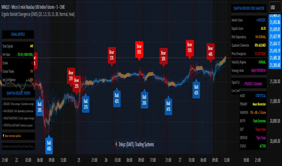
Ergodic Market Divergence (EMD)Ergodic Market Divergence (EMD)
Bridging Statistical Physics and Market Dynamics Through Ensemble Analysis
The Revolutionary Concept: When Physics Meets Trading
After months of research into ergodic theory—a fundamental principle in statistical mechanics—I've developed a trading system that identifies when markets transition between predictable and unpredictable states. This indicator doesn't just follow price; it analyzes whether current market behavior will persist or revert, giving traders a scientific edge in timing entries and exits.
The Core Innovation: Ergodic Theory Applied to Markets
What Makes Markets Ergodic or Non-Ergodic?
In statistical physics, ergodicity determines whether a system's future resembles its past. Applied to trading:
Ergodic Markets (Mean-Reverting)
- Time averages equal ensemble averages
- Historical patterns repeat reliably
- Price oscillates around equilibrium
- Traditional indicators work well
Non-Ergodic Markets (Trending)
- Path dependency dominates
- History doesn't predict future
- Price creates new equilibrium levels
- Momentum strategies excel
The Mathematical Framework
The Ergodic Score combines three critical divergences:
Ergodic Score = (Price Divergence × Market Stress + Return Divergence × 1000 + Volatility Divergence × 50) / 3
Where:
Price Divergence: How far current price deviates from market consensus
Return Divergence: Momentum differential between instrument and market
Volatility Divergence: Volatility regime misalignment
Market Stress: Adaptive multiplier based on current conditions
The Ensemble Analysis Revolution
Beyond Single-Instrument Analysis
Traditional indicators analyze one chart in isolation. EMD monitors multiple correlated markets simultaneously (SPY, QQQ, IWM, DIA) to detect systemic regime changes. This ensemble approach:
Reveals Hidden Divergences: Individual stocks may diverge from market consensus before major moves
Filters False Signals: Requires broader market confirmation
Identifies Regime Shifts: Detects when entire market structure changes
Provides Context: Shows if moves are isolated or systemic
Dynamic Threshold Adaptation
Unlike fixed-threshold systems, EMD's boundaries evolve with market conditions:
Base Threshold = SMA(Ergodic Score, Lookback × 3)
Adaptive Component = StDev(Ergodic Score, Lookback × 2) × Sensitivity
Final Threshold = Smoothed(Base + Adaptive)
This creates context-aware signals that remain effective across different market environments.
The Confidence Engine: Know Your Signal Quality
Multi-Factor Confidence Scoring
Every signal receives a confidence score based on:
Signal Clarity (0-35%): How decisively the ergodic threshold is crossed
Momentum Strength (0-25%): Rate of ergodic change
Volatility Alignment (0-20%): Whether volatility supports the signal
Market Quality (0-20%): Price convergence and path dependency factors
Real-Time Confidence Updates
The Live Confidence metric continuously updates, showing:
- Current opportunity quality
- Market state clarity
- Historical performance influence
- Signal recency boost
- Visual Intelligence System
Adaptive Ergodic Field Bands
Dynamic bands that expand and contract based on market state:
Primary Color: Ergodic state (mean-reverting)
Danger Color: Non-ergodic state (trending)
Band Width: Expected price movement range
Squeeze Indicators: Volatility compression warnings
Quantum Wave Ribbons
Triple EMA system (8, 21, 55) revealing market flow:
Compressed Ribbons: Consolidation imminent
Expanding Ribbons: Directional move developing
Color Coding: Matches current ergodic state
Phase Transition Signals
Clear entry/exit markers at regime changes:
Bull Signals: Ergodic restoration (mean reversion opportunity)
Bear Signals: Ergodic break (trend following opportunity)
Confidence Labels: Percentage showing signal quality
Visual Intensity: Stronger signals = deeper colors
Professional Dashboard Suite
Main Analytics Panel (Top Right)
Market State Monitor
- Current regime (Ergodic/Non-Ergodic)
- Ergodic score with threshold
- Path dependency strength
- Quantum coherence percentage
Divergence Metrics
- Price divergence with severity
- Volatility regime classification
- Strategy mode recommendation
- Signal strength indicator
Live Intelligence
- Real-time confidence score
- Color-coded risk levels
- Dynamic strategy suggestions
Performance Tracking (Left Panel)
Signal Analytics
- Total historical signals
- Win rate with W/L breakdown
- Current streak tracking
- Closed trade counter
Regime Analysis
- Current market behavior
- Bars since last signal
- Recommended actions
- Average confidence trends
Strategy Command Center (Bottom Right)
Adaptive Recommendations
- Active strategy mode
- Primary approach (mean reversion/momentum)
- Suggested indicators ("weapons")
- Entry/exit methodology
- Risk management guidance
- Comprehensive Input Guide
Core Algorithm Parameters
Analysis Period (10-100 bars)
Scalping (10-15): Ultra-responsive, more signals, higher noise
Day Trading (20-30): Balanced sensitivity and stability
Swing Trading (40-100): Smooth signals, major moves only Default: 20 - optimal for most timeframes
Divergence Threshold (0.5-5.0)
Hair Trigger (0.5-1.0): Catches every wiggle, many false signals
Balanced (1.5-2.5): Good signal-to-noise ratio
Conservative (3.0-5.0): Only extreme divergences Default: 1.5 - best risk/reward balance
Path Memory (20-200 bars)
Short Memory (20-50): Recent behavior focus, quick adaptation
Medium Memory (50-100): Balanced historical context
Long Memory (100-200): Emphasizes established patterns Default: 50 - captures sufficient history without lag
Signal Spacing (5-50 bars)
Aggressive (5-10): Allows rapid-fire signals
Normal (15-25): Prevents clustering, maintains flow
Conservative (30-50): Major setups only Default: 15 - optimal trade frequency
Ensemble Configuration
Select markets for consensus analysis:
SPY: Broad market sentiment
QQQ: Technology leadership
IWM: Small-cap risk appetite
DIA: Blue-chip stability
More instruments = stronger consensus but potentially diluted signals
Visual Customization
Color Themes (6 professional options):
Quantum: Cyan/Pink - Modern trading aesthetic
Matrix: Green/Red - Classic terminal look
Heat: Blue/Red - Temperature metaphor
Neon: Cyan/Magenta - High contrast
Ocean: Turquoise/Coral - Calming palette
Sunset: Red-orange/Teal - Warm gradients
Display Controls:
- Toggle each visual component
- Adjust transparency levels
- Scale dashboard text
- Show/hide confidence scores
- Trading Strategies by Market State
- Ergodic State Strategy (Primary Color Bands)
Market Characteristics
- Price oscillates predictably
- Support/resistance hold
- Volume patterns repeat
- Mean reversion dominates
Optimal Approach
Entry: Fade moves at band extremes
Target: Middle band (equilibrium)
Stop: Just beyond outer bands
Size: Full confidence-based position
Recommended Tools
- RSI for oversold/overbought
- Bollinger Bands for extremes
- Volume profile for levels
- Non-Ergodic State Strategy (Danger Color Bands)
Market Characteristics
- Price trends persistently
- Levels break decisively
- Volume confirms direction
- Momentum accelerates
Optimal Approach
Entry: Breakout from bands
Target: Trail with expanding bands
Stop: Inside opposite band
Size: Scale in with trend
Recommended Tools
- Moving average alignment
- ADX for trend strength
- MACD for momentum
- Advanced Features Explained
Quantum Coherence Metric
Measures phase alignment between individual and ensemble behavior:
80-100%: Perfect sync - strong mean reversion setup
50-80%: Moderate alignment - mixed signals
0-50%: Decoherence - trending behavior likely
Path Dependency Analysis
Quantifies how much history influences current price:
Low (<30%): Technical patterns reliable
Medium (30-50%): Mixed influences
High (>50%): Fundamental shift occurring
Volatility Regime Classification
Contextualizes current volatility:
Normal: Standard strategies apply
Elevated: Widen stops, reduce size
Extreme: Defensive mode required
Signal Strength Indicator
Real-time opportunity quality:
- Distance from threshold
- Momentum acceleration
- Cross-validation factors
Risk Management Framework
Position Sizing by Confidence
90%+ confidence = 100% position size
70-90% confidence = 75% position size
50-70% confidence = 50% position size
<50% confidence = 25% or skip
Dynamic Stop Placement
Ergodic State: ATR × 1.0 from entry
Non-Ergodic State: ATR × 2.0 from entry
Volatility Adjustment: Multiply by current regime
Multi-Timeframe Alignment
- Check higher timeframe regime
- Confirm ensemble consensus
- Verify volume participation
- Align with major levels
What Makes EMD Unique
Original Contributions
First Ergodic Theory Trading Application: Transforms abstract physics into practical signals
Ensemble Market Analysis: Revolutionary multi-market divergence system
Adaptive Confidence Engine: Institutional-grade signal quality metrics
Quantum Coherence: Novel market alignment measurement
Smart Signal Management: Prevents clustering while maintaining responsiveness
Technical Innovations
Dynamic Threshold Adaptation: Self-adjusting sensitivity
Path Memory Integration: Historical dependency weighting
Stress-Adjusted Scoring: Market condition normalization
Real-Time Performance Tracking: Built-in strategy analytics
Optimization Guidelines
By Timeframe
Scalping (1-5 min)
Period: 10-15
Threshold: 0.5-1.0
Memory: 20-30
Spacing: 5-10
Day Trading (5-60 min)
Period: 20-30
Threshold: 1.5-2.5
Memory: 40-60
Spacing: 15-20
Swing Trading (1H-1D)
Period: 40-60
Threshold: 2.0-3.0
Memory: 80-120
Spacing: 25-35
Position Trading (1D-1W)
Period: 60-100
Threshold: 3.0-5.0
Memory: 100-200
Spacing: 40-50
By Market Condition
Trending Markets
- Increase threshold
- Extend memory
- Focus on breaks
Ranging Markets
- Decrease threshold
- Shorten memory
- Focus on restores
Volatile Markets
- Increase spacing
- Raise confidence requirement
- Reduce position size
- Integration with Other Analysis
- Complementary Indicators
For Ergodic States
- RSI divergences
- Bollinger Band squeezes
- Volume profile nodes
- Support/resistance levels
For Non-Ergodic States
- Moving average ribbons
- Trend strength indicators
- Momentum oscillators
- Breakout patterns
- Fundamental Alignment
- Check economic calendar
- Monitor sector rotation
- Consider market themes
- Evaluate risk sentiment
Troubleshooting Guide
Too Many Signals:
- Increase threshold
- Extend signal spacing
- Raise confidence minimum
Missing Opportunities
- Decrease threshold
- Reduce signal spacing
- Check ensemble settings
Poor Win Rate
- Verify timeframe alignment
- Confirm volume participation
- Review risk management
Disclaimer
This indicator is for educational and informational purposes only. It does not constitute financial advice. Trading involves substantial risk of loss and is not suitable for all investors. Past performance does not guarantee future results.
The ergodic framework provides unique market insights but cannot predict future price movements with certainty. Always use proper risk management, conduct your own analysis, and never risk more than you can afford to lose.
This tool should complement, not replace, comprehensive trading strategies and sound judgment. Markets remain inherently unpredictable despite advanced analysis techniques.
Transform market chaos into trading clarity with Ergodic Market Divergence.
Created with passion for the TradingView community
Trade with insight. Trade with anticipation.
— Dskyz , for DAFE Trading Systems
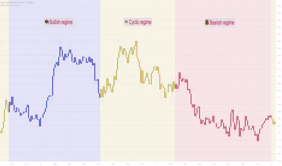
[GYTS-CE] Market Regime Detector🧊 Market Regime Detector (Community Edition)
🌸 Part of GoemonYae Trading System (GYTS) 🌸
🌸 --------- INTRODUCTION --------- 🌸
💮 What is the Market Regime Detector?
The Market Regime Detector is an advanced, consensus-based indicator that identifies the current market state to increase the probability of profitable trades. By distinguishing between trending (bullish or bearish) and cyclic (range-bound) market conditions, this detector helps you select appropriate tactics for different environments. Instead of forcing a single strategy across all market conditions, our detector allows you to adapt your approach based on real-time market behaviour.
💮 The Importance of Market Regimes
Markets constantly shift between different behavioural states or "regimes":
• Bullish trending markets - characterised by sustained upward price movement
• Bearish trending markets - characterised by sustained downward price movement
• Cyclic markets - characterised by range-bound, oscillating behaviour
Each regime requires fundamentally different trading approaches. Trend-following strategies excel in trending markets but fail in cyclic ones, while mean-reversion strategies shine in cyclic markets but underperform in trending conditions. Detecting these regimes is essential for successful trading, which is why we've developed the Market Regime Detector to accurately identify market states using complementary detection methods.
🌸 --------- KEY FEATURES --------- 🌸
💮 Consensus-Based Detection
Rather than relying on a single method, our detector employs two complementary detection methodologies that analyse different aspects of market behaviour:
• Dominant Cycle Average (DCA) - analyzes price movement relative to its lookback period, a proxy for the dominant cycle
• Volatility Channel - examines price behaviour within adaptive volatility bands
These diverse perspectives are synthesised into a robust consensus that minimises false signals while maintaining responsiveness to genuine regime changes.
💮 Dominant Cycle Framework
The Market Regime Detector uses the concept of dominant cycles to establish a reference framework. You can input the dominant cycle period that best represents the natural rhythm of your market, providing a stable foundation for regime detection across different timeframes.
💮 Intuitive Parameter System
We've distilled complex technical parameters into intuitive controls that traders can easily understand:
• Adaptability - how quickly the detector responds to changing market conditions
• Sensitivity - how readily the detector identifies transitions between regimes
• Consensus requirement - how much agreement is needed among detection methods
This approach makes the detector accessible to traders of all experience levels while preserving the power of the underlying algorithms.
💮 Visual Market Feedback
The detector provides clear visual feedback about the current market regime through:
• Colour-coded chart backgrounds (purple shades for bullish, pink for bearish, yellow for cyclic)
• Colour-coded price bars
• Strength indicators showing the degree of consensus
• Customizable colour schemes to match your preferences or trading system
💮 Integration in the GYTS suite
The Market Regime Detector is compatible with the GYTS Suite , i.e. it passes the regime into the 🎼 Order Orchestrator where you can set how to trade the trending and cyclic regime.
🌸 --------- CONFIGURATION SETTINGS --------- 🌸
💮 Adaptability
Controls how quickly the Market Regime detector adapts to changing market conditions. You can see it as a low-frequency, long-term change parameter:
Very Low: Very slow adaptation, most stable but may miss regime changes
Low: Slower adaptation, more stability but less responsiveness
Normal: Balanced between stability and responsiveness
High: Faster adaptation, more responsive but less stable
Very High: Very fast adaptation, highly responsive but may generate false signals
This setting affects lookback periods and filter parameters across all detection methods.
💮 Sensitivity
Controls how sensitive the detector is to market regime transitions. This acts as a high-frequency, short-term change parameter:
Very Low: Requires substantial evidence to identify a regime change
Low: Less sensitive, reduces false signals but may miss some transitions
Normal: Balanced sensitivity suitable for most markets
High: More sensitive, detects subtle regime changes but may have more noise
Very High: Very sensitive, detects minor fluctuations but may produce frequent changes
This setting affects thresholds for regime detection across all methods.
💮 Dominant Cycle Period
This parameter allows you to specify the market's natural rhythm in bars. This represents a complete market cycle (up and down movement). Finding the right value for your specific market and timeframe might require some experimentation, but it's a crucial parameter that helps the detector accurately identify regime changes. Most of the times the cycle is between 20 and 40 bars.
💮 Consensus Mode
Determines how the signals from both detection methods are combined to produce the final market regime:
• Any Method (OR) : Signals bullish/bearish if either method detects that regime. If methods conflict (one bullish, one bearish), the stronger signal wins. More sensitive, catches more regime changes but may produce more false signals.
• All Methods (AND) : Signals only when both methods agree on the regime. More conservative, reduces false signals but might miss some legitimate regime changes.
• Weighted Decision : Balances both methods with equal weighting. Provides a middle ground between sensitivity and stability.
Each mode also calculates a continuous regime strength value that's used for colour intensity in the 'unconstrained' display mode.
💮 Display Mode
Choose how to display the market regime colours:
• Unconstrained regime: Shows the regime strength as a continuous gradient. This provides more nuanced visualisation where the intensity of the colour indicates the strength of the trend.
• Consensus only: Shows only the final consensus regime with fixed colours based on the detected regime type.
The background and bar colours will change to indicate the current market regime:
• Purple shades: Bullish trending market (darker purple indicates stronger bullish trend)
• Pink shades: Bearish trending market (darker pink indicates stronger bearish trend)
• Yellow: Cyclic (range-bound) market
💮 Custom Colour Options
The Market Regime Detector allows you to customize the colour scheme to match your personal preferences or to coordinate with other indicators:
• Use custom colours: Toggle to enable your own colour choices instead of the default scheme
• Transparency: Adjust the transparency level of all regime colours
• Bullish colours: Define custom colours for strong, medium, weak, and very weak bullish trends
• Bearish colours: Define custom colours for strong, medium, weak, and very weak bearish trends
• Cyclic colour: Define a custom colour for cyclic (range-bound) market conditions
🌸 --------- DETECTION METHODS --------- 🌸
💮 Dominant Cycle Average (DCA)
The Dominant Cycle Average method forms a key part of our detection system:
1. Theoretical Foundation :
The DCA method builds on cycle analysis and the observation that in trending markets, price consistently remains on one side of a moving average calculated using the dominant cycle period. In contrast, during cyclic markets, price oscillates around this average.
2. Calculation Process :
• We calculate a Simple Moving Average (SMA) using the specified lookback period - a proxy for the dominant cycle period
• We then analyse the proportion of time that price spends above or below this SMA over a lookback window. The theory is that the price should cross the SMA each half cycle, assuming that the dominant cycle period is correct and price follows a sinusoid.
• This lookback window is adaptive, scaling with the dominant cycle period (controlled by the Adaptability setting)
• The different values are standardised and normalised to possess more resolving power and to be more robust to noise.
3. Regime Classification :
• When the normalised proportion exceeds a positive threshold (determined by Sensitivity setting), the market is classified as bullish trending
• When it falls below a negative threshold, the market is classified as bearish trending
• When the proportion remains between these thresholds, the market is classified as cyclic
💮 Volatility Channel
The Volatility Channel method complements the DCA method by focusing on price movement relative to adaptive volatility bands:
1. Theoretical Foundation :
This method is based on the observation that trending markets tend to sustain movement outside of normal volatility ranges, while cyclic markets tend to remain contained within these ranges. By creating adaptive bands that adjust to current market volatility, we can detect when price behaviour indicates a trending or cyclic regime.
2. Calculation Process :
• We first calculate a smooth base channel center using a low pass filter, creating a noise-reduced centreline for price
• True Range (TR) is used to measure market volatility, which is then smoothed and scaled by the deviation factor (controlled by Sensitivity)
• Upper and lower bands are created by adding and subtracting this scaled volatility from the centreline
• Price is smoothed using an adaptive A2RMA filter, which has a very flat and stable behaviour, to reduce noise while preserving trend characteristics
• The position of this smoothed price relative to the bands is continuously monitored
3. Regime Classification :
• When smoothed price moves above the upper band, the market is classified as bullish trending
• When smoothed price moves below the lower band, the market is classified as bearish trending
• When price remains between the bands, the market is classified as cyclic
• The magnitude of price's excursion beyond the bands is used to determine trend strength
4. Adaptive Behaviour :
• The smoothing periods and deviation calculations automatically adjust based on the Adaptability setting
• The measured volatility is calculated over a period proportional to the dominant cycle, ensuring the detector works across different timeframes
• Both the center line and the bands adapt dynamically to changing market conditions, making the detector responsive yet stable
This method provides a unique perspective that complements the DCA approach, with the consensus mechanism synthesising insights from both methods.
🌸 --------- USAGE GUIDE --------- 🌸
💮 Starting with Default Settings
The default settings (Normal for Adaptability and Sensitivity, Weighted Decision for Consensus Mode) provide a balanced starting point suitable for most markets and timeframes. Begin by observing how these settings identify regimes in your preferred instruments.
💮 Finding the Optimal Dominant Cycle
The dominant cycle period is a critical parameter. Here are some approaches to finding an appropriate value:
• Start with typical values, usually something around 25 works well
• Visually identify the average distance between significant peaks and troughs
• Experiment with different values and observe which provides the most stable regime identification
• Consider using cycle-finding indicators to help identify the natural rhythm of your market
💮 Adjusting Parameters
• If you notice too many regime changes → Decrease Sensitivity or increase Consensus requirement
• If regime changes seem delayed → Increase Adaptability
• If a trending regime is not detected, the market is automatically assigned to be in a cyclic state
• If you want to see more nuanced regime transitions → Try the "unconstrained" display mode (note that this will not affect the output to other indicators)
💮 Trading Applications
Regime-Specific Strategies:
• Bullish Trending Regime - Use trend-following strategies, trail stops wider, focus on breakouts, consider holding positions longer, and emphasize buying dips
• Bearish Trending Regime - Consider shorts, tighter stops, focus on breakdown points, sell rallies, implement downside protection, and reduce position sizes
• Cyclic Regime - Apply mean-reversion strategies, trade range boundaries, apply oscillators, target definable support/resistance levels, and use profit-taking at extremes
Strategy Switching:
Create a set of rules for each market regime and switch between them based on the detector's signal. This approach can significantly improve performance compared to applying a single strategy across all market conditions.
GYTS Suite Integration:
• In the GYTS 🎼 Order Orchestrator, select the '🔗 STREAM-int 🧊 Market Regime' as the market regime source
• Note that the consensus output (i.e. not the "unconstrained" display) will be used in this stream
• Create different strategies for trending (bullish/bearish) and cyclic regimes. The GYTS 🎼 Order Orchestrator is specifically made for this.
• The output stream is actually very simple, and can possibly be used in indicators and strategies as well. It outputs 1 for bullish, -1 for bearish and 0 for cyclic regime.
🌸 --------- FINAL NOTES --------- 🌸
💮 Development Philosophy
The Market Regime Detector has been developed with several key principles in mind:
1. Robustness - The detection methods have been rigorously tested across diverse markets and timeframes to ensure reliable performance.
2. Adaptability - The detector automatically adjusts to changing market conditions, requiring minimal manual intervention.
3. Complementarity - Each detection method provides a unique perspective, with the collective consensus being more reliable than any individual method.
4. Intuitiveness - Complex technical parameters have been abstracted into easily understood controls.
💮 Ongoing Refinement
The Market Regime Detector is under continuous development. We regularly:
• Fine-tune parameters based on expanded market data
• Research and integrate new detection methodologies
• Optimise computational efficiency for real-time analysis
Your feedback and suggestions are very important in this ongoing refinement process!
three Supertrend EMA Strategy by Prasanna +DhanuThe indicator described in your Pine Script is a Supertrend EMA Strategy that combines the Supertrend and EMA (Exponential Moving Average) to create a trend-following strategy. Here’s a detailed breakdown of how this indicator works:
1. EMA (Exponential Moving Average):
The EMA is a moving average that places more weight on recent prices, making it more responsive to price changes compared to a simple moving average (SMA). In this strategy, the EMA is used to determine the overall trend direction.
Input Parameter:
ema_length: This is the period for the EMA, set to 50 periods by default. A shorter EMA will respond more quickly to price movements, while a longer EMA is smoother and less sensitive to short-term fluctuations.
How it's used:
If the price is above the EMA, it indicates an uptrend.
If the price is below the EMA, it indicates a downtrend.
2. Supertrend Indicator:
The Supertrend indicator is a trend-following tool based on the Average True Range (ATR), which is a volatility measure. It helps to identify the direction of the trend by setting a dynamic support or resistance level.
Input Parameters:
supertrend_atr_period: The period used for calculating the ATR, set to 10 periods by default.
supertrend_multiplier1: Multiplier for the first Supertrend, set to 3.0.
supertrend_multiplier2: Multiplier for the second Supertrend, set to 2.0.
supertrend_multiplier3: Multiplier for the third Supertrend, set to 1.0.
Each Supertrend line has a different multiplier, which affects its sensitivity to price changes. The ATR period defines how many periods of price data are used to calculate the ATR.
How the Supertrend works:
If the Supertrend value is below the price, the trend is considered bullish (uptrend).
If the Supertrend value is above the price, the trend is considered bearish (downtrend).
The Supertrend will switch between up and down based on price movement and ATR, providing a dynamic trend-following signal.
3. Three Supertrend Lines:
In this strategy, three Supertrend lines are calculated with different multipliers and the same ATR period (10 periods). Each line is more or less sensitive to price changes, and they are plotted on the chart in different colors based on whether the trend is bullish (green) or bearish (red).
Supertrend 1: The most sensitive Supertrend with a multiplier of 3.0.
Supertrend 2: A moderately sensitive Supertrend with a multiplier of 2.0.
Supertrend 3: The least sensitive Supertrend with a multiplier of 1.0.
Each Supertrend line signals a bullish trend when its value is below the price and a bearish trend when its value is above the price.
4. Strategy Rules:
This strategy uses the three Supertrend lines combined with the EMA to generate trade signals.
Entry Conditions:
A long entry is triggered when all three Supertrend lines are in an uptrend (i.e., all three Supertrend lines are below the price), and the price is above the EMA. This suggests a strong bullish market condition.
A short entry is triggered when all three Supertrend lines are in a downtrend (i.e., all three Supertrend lines are above the price), and the price is below the EMA. This suggests a strong bearish market condition.
Exit Conditions:
A long exit occurs when the third Supertrend (the least sensitive one) switches to a downtrend (i.e., the price falls below it).
A short exit occurs when the third Supertrend switches to an uptrend (i.e., the price rises above it).
5. Visualization:
The strategy also plots the following on the chart:
The EMA is plotted as a blue line, which helps identify the overall trend.
The three Supertrend lines are plotted with different colors:
Supertrend 1: Green (for uptrend) and Red (for downtrend).
Supertrend 2: Green (for uptrend) and Red (for downtrend).
Supertrend 3: Green (for uptrend) and Red (for downtrend).
Summary of the Strategy:
The strategy combines three Supertrend indicators (with different multipliers) and an EMA to capture both short-term and long-term trends.
Long positions are entered when all three Supertrend lines are bullish and the price is above the EMA.
Short positions are entered when all three Supertrend lines are bearish and the price is below the EMA.
Exits occur when the third Supertrend line (the least sensitive) signals a change in trend direction.
This combination of indicators allows for a robust trend-following strategy that adapts to both short-term volatility and long-term trend direction. The Supertrend lines provide quick reaction to price changes, while the EMA offers a smoother, more stable trend direction for confirmation.
The indicator described in your Pine Script is a Supertrend EMA Strategy that combines the Supertrend and EMA (Exponential Moving Average) to create a trend-following strategy. Here’s a detailed breakdown of how this indicator works:
1. EMA (Exponential Moving Average):
The EMA is a moving average that places more weight on recent prices, making it more responsive to price changes compared to a simple moving average (SMA). In this strategy, the EMA is used to determine the overall trend direction.
Input Parameter:
ema_length: This is the period for the EMA, set to 50 periods by default. A shorter EMA will respond more quickly to price movements, while a longer EMA is smoother and less sensitive to short-term fluctuations.
How it's used:
If the price is above the EMA, it indicates an uptrend.
If the price is below the EMA, it indicates a downtrend.
2. Supertrend Indicator:
The Supertrend indicator is a trend-following tool based on the Average True Range (ATR), which is a volatility measure. It helps to identify the direction of the trend by setting a dynamic support or resistance level.
Input Parameters:
supertrend_atr_period: The period used for calculating the ATR, set to 10 periods by default.
supertrend_multiplier1: Multiplier for the first Supertrend, set to 3.0.
supertrend_multiplier2: Multiplier for the second Supertrend, set to 2.0.
supertrend_multiplier3: Multiplier for the third Supertrend, set to 1.0.
Each Supertrend line has a different multiplier, which affects its sensitivity to price changes. The ATR period defines how many periods of price data are used to calculate the ATR.
How the Supertrend works:
If the Supertrend value is below the price, the trend is considered bullish (uptrend).
If the Supertrend value is above the price, the trend is considered bearish (downtrend).
The Supertrend will switch between up and down based on price movement and ATR, providing a dynamic trend-following signal.
3. Three Supertrend Lines:
In this strategy, three Supertrend lines are calculated with different multipliers and the same ATR period (10 periods). Each line is more or less sensitive to price changes, and they are plotted on the chart in different colors based on whether the trend is bullish (green) or bearish (red).
Supertrend 1: The most sensitive Supertrend with a multiplier of 3.0.
Supertrend 2: A moderately sensitive Supertrend with a multiplier of 2.0.
Supertrend 3: The least sensitive Supertrend with a multiplier of 1.0.
Each Supertrend line signals a bullish trend when its value is below the price and a bearish trend when its value is above the price.
4. Strategy Rules:
This strategy uses the three Supertrend lines combined with the EMA to generate trade signals.
Entry Conditions:
A long entry is triggered when all three Supertrend lines are in an uptrend (i.e., all three Supertrend lines are below the price), and the price is above the EMA. This suggests a strong bullish market condition.
A short entry is triggered when all three Supertrend lines are in a downtrend (i.e., all three Supertrend lines are above the price), and the price is below the EMA. This suggests a strong bearish market condition.
Exit Conditions:
A long exit occurs when the third Supertrend (the least sensitive one) switches to a downtrend (i.e., the price falls below it).
A short exit occurs when the third Supertrend switches to an uptrend (i.e., the price rises above it).
5. Visualization:
The strategy also plots the following on the chart:
The EMA is plotted as a blue line, which helps identify the overall trend.
The three Supertrend lines are plotted with different colors:
Supertrend 1: Green (for uptrend) and Red (for downtrend).
Supertrend 2: Green (for uptrend) and Red (for downtrend).
Supertrend 3: Green (for uptrend) and Red (for downtrend).
Summary of the Strategy:
The strategy combines three Supertrend indicators (with different multipliers) and an EMA to capture both short-term and long-term trends.
Long positions are entered when all three Supertrend lines are bullish and the price is above the EMA.
Short positions are entered when all three Supertrend lines are bearish and the price is below the EMA.
Exits occur when the third Supertrend line (the least sensitive) signals a change in trend direction.
This combination of indicators allows for a robust trend-following strategy that adapts to both short-term volatility and long-term trend direction. The Supertrend lines provide quick reaction to price changes, while the EMA offers a smoother, more stable trend direction for confirmation.

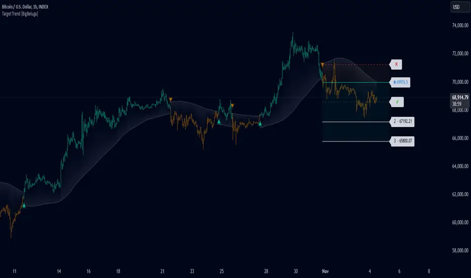
Target Trend [BigBeluga]The Target Trend indicator is a trend-following tool designed to assist traders in capturing directional moves while managing entry, stop loss, and profit targets visually on the chart. Using adaptive SMA bands as the core trend detection method, this indicator dynamically identifies shifts in trend direction and provides structured exit points through customizable target levels.
SP500:
🔵 IDEA
The Target Trend indicator’s concept is to simplify trade management by providing automated visual cues for entries, stops, and targets directly on the chart. When a trend change is detected, the indicator prints an up or down triangle to signal entry direction, plots three customizable target levels for potential exits, and calculates a stop-loss level below or above the entry point. The indicator continuously adapts as price moves, making it easier for traders to follow and manage trades in real time.
When price crosses a target level, the label changes to a check mark, confirming that the target has been achieved. Similarly, if the stop-loss level is hit, the label changes to an "X," and the line becomes dashed, indicating that the stop loss has been activated. This feature provides traders with a clear visual trail of whether their targets or stop loss have been hit, allowing for easier trade tracking and exit strategy management.
🔵 KEY FEATURES & USAGE
SMA Bands for Trend Detection: The indicator uses adaptive SMA bands to identify the trend direction. When price crosses above or below these bands, a new trend is detected, triggering entry signals. The entry point is marked on the chart with a triangle symbol, which updates with each new trend change.
Automated Targets and Stop Loss Management: Upon a new trend signal, the indicator automatically plots three price targets and a stop loss level. These levels provide traders with structured exit points for potential gains and a clear risk limit. The stop loss is placed below or above the entry point, depending on the trend direction, to manage downside risk effectively.
Visual Target and Stop Loss Validation: As price hits each target, the label beside the level updates to a check mark, indicating that the target has been reached. Similarly, if the stop loss is activated, the stop loss label changes to an "X," and the line becomes dashed. This feature visually confirms whether targets or stop losses are hit, simplifying trade management.
The indicator also marks the entry price at each trend change with a label on the chart, allowing traders to quickly see their initial entry point relative to current price and target levels.
🔵 CUSTOMIZATION
Trend Length: Set the lookback period for the trend-detection SMA bands to adjust the sensitivity to trend changes.
Targets Setting: Customize the number and spacing of the targets to fit your trading style and market conditions.
Visual Styles: Adjust the appearance of labels, lines, and symbols on the chart for a clearer view and personalized layout.
🔵 CONCLUSION
The Target Trend indicator offers a streamlined approach to trend trading by integrating entry, target, and stop loss management into a single visual tool. With automatic tracking of target levels and stop loss hits, it helps traders stay focused on the current trend while keeping track of risk and reward with minimal effort.
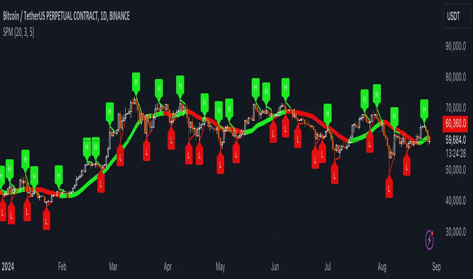
Uptrick: SMA Pivot Marker### Uptrick: SMA Pivot Marker (SPM) — Extensive Guide
#### Introduction
The **Uptrick: SMA Pivot Marker (SPM)** is a sophisticated technical analysis tool crafted by Uptrick to help traders interpret market trends and identify key price levels where significant reversals might occur. By integrating the principles of the Simple Moving Average (SMA) with pivot point analysis, the SPM offers a comprehensive approach to understanding market dynamics. This extensive guide explores the purpose, functionality, and practical applications of the SPM, providing an in-depth analysis of its features, settings, and usage across various trading strategies.
#### Purpose of the SPM
The **SMA Pivot Marker (SPM)** aims to enhance trading strategies by offering a dual approach to market analysis:
1. **Trend Identification**:
- **Objective**: To discern the prevailing market direction and guide trading decisions based on the overall trend.
- **Method**: Utilizes the SMA to smooth out price fluctuations, providing a clearer picture of the trend. This helps traders align their trades with the market's direction, increasing the probability of successful trades.
2. **Pivot Point Detection**:
- **Objective**: To identify key levels where the price is likely to reverse, providing potential support and resistance zones.
- **Method**: Calculates and marks pivot highs and lows, which are significant price points where previous trends have reversed. These levels are used to predict future price movements and establish trading strategies.
3. **Trend Change Alerts**:
- **Objective**: To notify traders of potential shifts in market direction, enabling timely adjustments to trading positions.
- **Method**: Detects and highlights crossover and crossunder points of the smoothed line, indicating possible trend changes. This helps traders react promptly to changing market conditions.
#### Detailed Functionality
1. **Smoothing Line Calculation**:
- **Simple Moving Average (SMA)**:
- **Definition**: The SMA is a type of moving average that calculates the average of a security’s price over a specified number of periods. It smooths out price data to filter out short-term fluctuations and highlight the longer-term trend.
- **Calculation**: The SMA is computed by summing the closing prices of the chosen number of periods and then dividing by the number of periods. For example, a 20-period SMA adds the closing prices for the past 20 periods and divides by 20.
- **Purpose**: The SMA helps in identifying the direction of the trend. A rising SMA indicates an uptrend, while a falling SMA indicates a downtrend. This smoothing helps traders to avoid being misled by short-term price noise.
2. **Pivot Points Calculation**:
- **Pivot Highs and Lows**:
- **Definition**: Pivot points are significant price levels where a market trend is likely to reverse. A pivot high is the highest price over a certain period, surrounded by lower prices on both sides, while a pivot low is the lowest price surrounded by higher prices.
- **Calculation**: The SPM calculates pivot points based on a user-defined lookback period. For instance, if the lookback period is set to 3, the indicator will find the highest and lowest prices within the past 3 periods and mark these points.
- **Purpose**: Pivot points are used to identify potential support and resistance levels. Traders often use these levels to set entry and exit points, stop-loss orders, and to gauge market sentiment.
3. **Visualization**:
- **Smoothed Line Plot**:
- **Description**: The smoothed line, calculated using the SMA, is plotted on the chart to provide a visual representation of the trend. This line adjusts its color based on the trend direction, helping traders quickly assess the market condition.
- **Color Coding**: The smoothed line is colored green (upColor) when it is rising, indicating a bullish trend, and red (downColor) when it is falling, indicating a bearish trend. This color-coding helps traders visually differentiate between uptrends and downtrends.
- **Line Width**: The width of the line can be adjusted to improve visibility. A thicker line may be more noticeable, while a thinner line might provide a cleaner look on the chart.
- **Pivot Markers**:
- **Description**: Pivot highs and lows are marked on the chart with lines and labels. These markers help in visually identifying significant price levels.
- **Color and Labels**: Pivot highs are represented with green lines and labels ("H"), while pivot lows are marked with red lines and labels ("L"). This color scheme and labeling make it easy to distinguish between resistance (highs) and support (lows).
4. **Trend Change Detection**:
- **Trend Up**:
- **Detection**: The indicator identifies an upward trend change when the smoothed line crosses above its previous value. This crossover suggests a potential shift from a downtrend to an uptrend.
- **Usage**: Traders can interpret this signal as a potential buying opportunity or an indication to review and possibly adjust their trading positions to align with the new uptrend.
- **Trend Down**:
- **Detection**: A downward trend change is detected when the smoothed line crosses below its previous value. This crossunder indicates a potential shift from an uptrend to a downtrend.
- **Usage**: This signal can be used to consider selling opportunities or to reassess long positions in light of the emerging downtrend.
#### User Inputs
1. **Smoothing Period**:
- **Description**: This input determines the number of periods over which the SMA is calculated. It directly affects the smoothness of the line and the sensitivity of trend detection.
- **Range**: The smoothing period can be set to any integer value greater than or equal to 1. There is no specified upper limit, offering flexibility for various trading styles.
- **Default Value**: The default smoothing period is 20, which is a common choice for medium-term trend analysis.
- **Impact**: A longer smoothing period results in a smoother line, filtering out more noise and highlighting long-term trends. A shorter period makes the line more responsive to recent price changes, which can be useful for short-term trading strategies.
2. **Pivot Lookback**:
- **Description**: This input specifies the number of periods used to calculate the pivot highs and lows. It influences the sensitivity of pivot point detection and the relevance of the identified levels.
- **Range**: The pivot lookback period can be set to any integer value greater than or equal to 1, with no upper limit. Traders can adjust this parameter based on their trading timeframe and preferences.
- **Default Value**: The default lookback period is 3, which provides a balance between detecting significant pivots and avoiding excessive noise.
- **Impact**: A longer lookback period generates more stable pivot points, suitable for identifying long-term support and resistance levels. A shorter lookback period results in more frequent and recent pivot points, useful for intraday trading and quick responses to price changes.
#### Applications for Different Traders
1. **Trend Followers**:
- **Using the SMA**: Trend followers utilize the smoothed line to gauge the direction of the market. By aligning trades with the direction of the SMA, traders can capitalize on sustained trends and improve their chances of success.
- **Trend Change Alerts**: The trend change markers alert trend followers to potential shifts in market direction. These alerts help traders make timely decisions to enter or exit positions, ensuring they stay aligned with the prevailing trend.
2. **Reversal Traders**:
- **Pivot Points**: Reversal traders focus on pivot highs and lows to identify potential reversal points in the market. These points indicate where the market has previously reversed direction, providing potential entry and exit levels for trades.
- **Pivot Markers**: The visual markers for pivot highs and lows serve as clear signals for reversal traders. By monitoring these levels, traders can anticipate price reversals and plan their trades to exploit these opportunities.
3. **Swing Traders**:
- **Combining SMA and Pivot Points**: Swing traders can use the combination of the smoothed line and pivot points to identify medium-term trading opportunities. The smoothed line helps in understanding the broader trend, while pivot points provide specific levels for potential swings.
- **Trend Change Alerts**: Trend change markers help swing traders spot new swing opportunities as the market shifts direction. These markers provide potential entry points for swing trades and help traders adjust their strategies to capitalize on market movements.
4. **Scalpers**:
- **Short-Term Analysis**: Scalpers benefit from the short-term signals provided by the SPM. The smoothed line and pivot points offer insights into rapid price movements, while the trend change markers highlight quick trading opportunities.
- **Pivot Points**: For scalpers, pivot points are particularly useful in identifying key levels where price may reverse within a short time frame. By focusing on these levels, scalpers can plan trades with tight stop-loss orders and capitalize on quick price changes.
#### Implementation and Best Practices
1. **Setting Parameters**:
- **Smoothing Period**: Adjust the smoothing period according to your trading strategy and market conditions. For long-term analysis, use a longer period to filter out noise and highlight broader trends. For short-term trading, a shorter period provides more immediate insights into price movements.
- **Pivot Lookback**: Choose a lookback period that matches your trading timeframe. For intraday trading, a shorter lookback period offers quick identification of recent price levels. For swing trading or long-term strategies, a longer lookback period provides more stable pivot points.
2. **Combining with Other Indicators**:
- **Integration with Technical Tools**: The SPM can be used in conjunction with other technical indicators to enhance trading decisions. For instance, combining the
SPM with indicators like RSI (Relative Strength Index) or MACD (Moving Average Convergence Divergence) can provide additional confirmation for trend signals and pivot points.
- **Support and Resistance**: Integrate the SPM’s pivot points with other support and resistance levels to gain a comprehensive view of market conditions. This combined approach helps in identifying stronger levels of support and resistance, improving trade accuracy.
3. **Backtesting**:
- **Historical Performance**: Conduct backtesting with historical data to evaluate the effectiveness of the SPM. Analyze past performance to fine-tune the smoothing period and pivot lookback settings, ensuring they align with your trading style and market conditions.
- **Scenario Analysis**: Test the SPM under various market scenarios to understand its performance in different conditions. This analysis helps in assessing the reliability of the indicator and making necessary adjustments for diverse market environments.
4. **Customization**:
- **Visual Adjustments**: Customize the appearance of the smoothed line and pivot markers to enhance chart readability and match personal preferences. Clear visual representation of these elements improves the effectiveness of the indicator.
- **Alert Configuration**: Set up alerts for trend changes to receive timely notifications. Alerts help traders act quickly on potential market shifts without constant monitoring, allowing for more efficient trading decisions.
#### Conclusion
The **Uptrick: SMA Pivot Marker (SPM)** is a versatile and powerful technical analysis tool that combines the benefits of the Simple Moving Average with pivot point analysis. By providing insights into market trends, identifying key reversal points, and detecting trend changes, the SPM caters to a wide range of trading strategies, including trend following, reversal trading, swing trading, and scalping.
With its customizable inputs, visual markers, and trend change alerts, the SPM offers traders the flexibility to adapt the indicator to different market conditions and trading styles. Whether used independently or in conjunction with other technical tools, the SPM is designed to enhance trading decision-making and improve overall trading performance. By mastering the use of the SPM, traders can gain a valuable edge in navigating the complexities of financial markets and making more informed trading decisions.
Uptrick: Trend SMA Oscillator### In-Depth Analysis of the "Uptrick: Trend SMA Oscillator" Indicator
---
#### Introduction to the Indicator
The "Uptrick: Trend SMA Oscillator" is an advanced yet user-friendly technical analysis tool designed to help traders across all levels of experience identify and follow market trends with precision. This indicator builds upon the fundamental principles of the Simple Moving Average (SMA), a cornerstone of technical analysis, to deliver a clear, visually intuitive overlay on the price chart. Through its strategic use of color-coding and customizable parameters, the Uptrick: Trend SMA Oscillator provides traders with actionable insights into market dynamics, enhancing their ability to make informed trading decisions.
#### Core Concepts and Methodology
1. **Foundational Principle – Simple Moving Average (SMA):**
- The Simple Moving Average (SMA) is the heart of the Uptrick: Trend SMA Oscillator. The SMA is a widely-used technical indicator that calculates the average price of an asset over a specified number of periods. By smoothing out price data, the SMA helps to reduce the noise from short-term fluctuations, providing a clearer picture of the overall trend.
- In the Uptrick: Trend SMA Oscillator, two SMAs are employed:
- **Primary SMA (oscValue):** This is applied to the closing price of the asset over a user-defined period (default is 14 periods). This SMA tracks the price closely and is sensitive to changes in market direction.
- **Smoothing SMA (oscV):** This second SMA is applied to the primary SMA, further smoothing the data and helping to filter out minor price movements that might otherwise be mistaken for trend reversals. The default period for this smoothing is 50, but it can be adjusted to suit the trader's preference.
2. **Color-Coding for Trend Visualization:**
- One of the most distinctive features of this indicator is its use of color to represent market trends. The indicator’s line changes color based on the relationship between the primary SMA and the smoothing SMA:
- **Bullish (Green):** The line turns green when the primary SMA is equal to or greater than the smoothing SMA, indicating that the market is in an upward trend.
- **Bearish (Red):** Conversely, the line turns red when the primary SMA falls below the smoothing SMA, signaling a downward trend.
- This color-coded system provides traders with an immediate, easy-to-interpret visual cue about the market’s direction, allowing for quick decision-making.
#### Detailed Explanation of Inputs
1. **Bullish Color (Default: Green #00ff00):**
- This input allows traders to customize the color that represents bullish trends on the chart. The default setting is green, a color commonly associated with upward market movement. However, traders can adjust this to any color that suits their visual preferences or matches their overall chart theme.
2. **Bearish Color (Default: Red RGB: 245, 0, 0):**
- The bearish color input determines the color of the line when the market is trending downwards. The default setting is a vivid red, signaling caution or selling opportunities. Like the bullish color, this can be customized to fit the trader’s needs.
3. **Line Thickness (Default: 5):**
- This setting controls the thickness of the line plotted by the indicator. The default thickness of 5 makes the line prominent on the chart, ensuring that the trend is easily visible even in complex or crowded chart setups. Traders can adjust the thickness to make the line thinner or thicker, depending on their visual preferences.
4. **Primary SMA Period (Value 1 - Default: 14):**
- The primary SMA period defines how many periods (e.g., days, hours) are used to calculate the moving average based on the asset’s closing prices. The default period of 14 is a balanced setting that offers a good mix of responsiveness and stability, but traders can adjust this depending on their trading style:
- **Shorter Periods (e.g., 5-10):** These make the indicator more sensitive, capturing trends more quickly but also increasing the likelihood of reacting to short-term price fluctuations or "noise."
- **Longer Periods (e.g., 20-50):** These smooth the data more, providing a more stable trend line that is less prone to whipsaws but may be slower to respond to trend changes.
5. **Smoothing SMA Period (Value 2 - Default: 50):**
- The smoothing SMA period determines how much the primary SMA is smoothed. A longer smoothing period results in a more gradual, stable line that focuses on the broader trend. The default of 50 is designed to smooth out most of the short-term fluctuations while still being responsive enough to detect significant trend shifts.
- **Customization:**
- **Shorter Smoothing Periods (e.g., 20-30):** Make the indicator more responsive, better for fast-moving markets or for traders who want to capture quick trends.
- **Longer Smoothing Periods (e.g., 70-100):** Enhance stability, ideal for long-term traders looking to avoid reacting to minor price movements.
#### Unique Characteristics and Advantages
1. **Simplicity and Clarity:**
- The Uptrick: Trend SMA Oscillator’s design prioritizes simplicity without sacrificing effectiveness. By relying on the widely understood SMA, it avoids the complexity of more esoteric indicators while still providing reliable trend signals. This simplicity makes it accessible to traders of all levels, from novices who are just learning about technical analysis to experienced traders looking for a straightforward, dependable tool.
2. **Visual Feedback Mechanism:**
- The indicator’s use of color to signify market trends is a particularly powerful feature. This visual feedback mechanism allows traders to assess market conditions at a glance. The clarity of the green and red color scheme reduces the mental effort required to interpret the indicator, freeing the trader to focus on strategy execution.
3. **Adaptability Across Markets and Timeframes:**
- One of the strengths of the Uptrick: Trend SMA Oscillator is its versatility. The basic principles of moving averages apply equally well across different asset classes and timeframes. Whether trading stocks, forex, commodities, or cryptocurrencies, traders can use this indicator to gain insights into market trends.
- **Intraday Trading:** For day traders who operate on short timeframes (e.g., 1-minute, 5-minute charts), the oscillator can be adjusted to be more responsive, capturing quick shifts in momentum.
- **Swing Trading:** Swing traders, who typically hold positions for several days to weeks, will find the default settings or slightly adjusted periods ideal for identifying and riding medium-term trends.
- **Long-Term Trading:** Position traders and investors can adjust the indicator to focus on long-term trends by increasing the periods for both the primary and smoothing SMAs, filtering out minor fluctuations and highlighting sustained market movements.
4. **Minimal Lag:**
- One of the challenges with moving averages is lag—the delay between when the price changes and when the indicator reflects this change. The Uptrick: Trend SMA Oscillator addresses this by allowing traders to adjust the periods to find a balance between responsiveness and stability. While all SMAs inherently have some lag, the customizable nature of this indicator helps traders mitigate this effect to align with their specific trading goals.
5. **Customizable and Intuitive:**
- While many technical indicators come with a fixed set of parameters, the Uptrick: Trend SMA Oscillator is fully customizable, allowing traders to tailor it to their trading style, market conditions, and personal preferences. This makes it a highly flexible tool that can be adjusted as markets evolve or as a trader’s strategy changes over time.
#### Practical Applications for Different Trader Profiles
1. **Day Traders:**
- **Use Case:** Day traders can customize the SMA periods to create a faster, more responsive indicator. This allows them to capture short-term trends and make quick decisions. For example, reducing the primary SMA to 5 and the smoothing SMA to 20 can help day traders react promptly to intraday price movements.
- **Strategy Integration:** Day traders might use the Uptrick: Trend SMA Oscillator in conjunction with volume-based indicators to confirm the strength of a trend before entering or exiting trades.
2. **Swing Traders:**
- **Use Case:** Swing traders can use the default settings or slightly adjust them to smooth out minor price fluctuations while still capturing medium-term trends. This approach helps in identifying the optimal points to enter or exit trades based on the broader market direction.
- **Strategy Integration:** Swing traders can combine this indicator with oscillators like the Relative Strength Index (RSI) to confirm overbought or oversold conditions, thereby refining their entry and exit strategies.
3. **Position Traders:**
- **Use Case:** Position traders, who hold trades for extended periods, can extend the SMA periods to focus on long-term trends. By doing so, they minimize the impact of short-term market noise and focus on the underlying trend.
- **Strategy Integration:** Position traders might use the Uptrick: Trend SMA Oscillator in combination with fundamental analysis. The indicator can help confirm the timing of entries and exits based on broader economic or corporate developments.
4. **Algorithmic and Quantitative Traders:**
- **Use Case:** The simplicity and clear logic of the Uptrick: Trend SMA Oscillator make it an excellent candidate for algorithmic trading strategies. Its binary output—bullish or bearish—can be easily coded into automated trading systems.
- **Strategy Integration:** Quant traders might use the indicator as part of a larger trading system that incorporates multiple indicators and rules, optimizing the SMA periods based on historical backtesting to achieve the best results.
5. **Novice Traders:**
- **Use Case:** Beginners can use the Uptrick: Trend SMA Oscillator to learn the basics of trend-following strategies.
The visual simplicity of the color-coded line helps novice traders quickly understand market direction without the need to interpret complex data.
- **Educational Value:** The indicator serves as an excellent starting point for those new to technical analysis, providing a practical example of how moving averages work in a real-world trading environment.
#### Combining the Indicator with Other Tools
1. **Relative Strength Index (RSI):**
- The RSI is a momentum oscillator that measures the speed and change of price movements. When combined with the Uptrick: Trend SMA Oscillator, traders can look for instances where the RSI shows divergence from the price while the oscillator confirms the trend. This can be a powerful signal of an impending reversal or continuation.
2. **Moving Average Convergence Divergence (MACD):**
- The MACD is another popular trend-following momentum indicator. By using it alongside the Uptrick: Trend SMA Oscillator, traders can confirm the strength of a trend and identify potential entry and exit points with greater confidence. For example, a bullish crossover on the MACD that coincides with the Uptrick: Trend SMA Oscillator turning green can be a strong buy signal.
3. **Volume Indicators:**
- Volume is often considered the fuel behind price movements. Using volume indicators like the On-Balance Volume (OBV) or Volume Weighted Average Price (VWAP) in conjunction with the Uptrick: Trend SMA Oscillator can help traders confirm the validity of a trend. A trend identified by the oscillator that is supported by increasing volume is typically more reliable.
4. **Fibonacci Retracement:**
- Fibonacci retracement levels are used to identify potential reversal levels in a trending market. When the Uptrick: Trend SMA Oscillator indicates a trend, traders can use Fibonacci retracement levels to find potential entry points that align with the broader trend direction.
#### Implementation in Different Market Conditions
1. **Trending Markets:**
- The Uptrick: Trend SMA Oscillator excels in trending markets, where it provides clear signals on the direction of the trend. In a strong uptrend, the line will remain green, helping traders stay in the trade for longer periods. In a downtrend, the red line will signal the continuation of bearish conditions, prompting traders to stay short or avoid long positions.
2. **Sideways or Range-Bound Markets:**
- In range-bound markets, where price oscillates within a confined range without a clear trend, the Uptrick: Trend SMA Oscillator may produce more frequent changes in color. While this could indicate potential reversals at the range boundaries, traders should be cautious of false signals. It may be beneficial to pair the oscillator with a volatility indicator to better navigate such conditions.
3. **Volatile Markets:**
- In highly volatile markets, where prices can swing rapidly, the sensitivity of the Uptrick: Trend SMA Oscillator can be adjusted by modifying the SMA periods. A shorter SMA period might capture quick trends, but traders should be aware of the increased risk of whipsaws. Combining the oscillator with a volatility filter or using it in a higher time frame might help mitigate some of this risk.
#### Final Thoughts
The "Uptrick: Trend SMA Oscillator" is a versatile, easy-to-use indicator that stands out for its simplicity, visual clarity, and adaptability. It provides traders with a straightforward method to identify and follow market trends, using the well-established concept of moving averages. The indicator’s customizable nature makes it suitable for a wide range of trading styles, from day trading to long-term investing, and across various asset classes.
By offering immediate visual feedback through color-coded signals, the Uptrick: Trend SMA Oscillator simplifies the decision-making process, allowing traders to focus on execution rather than interpretation. Whether used on its own or as part of a broader technical analysis toolkit, this indicator has the potential to enhance trading strategies and improve overall performance.
Its accessibility and ease of use make it particularly appealing to novice traders, while its adaptability and reliability ensure that it remains a valuable tool for more experienced market participants. As markets continue to evolve, the Uptrick: Trend SMA Oscillator remains a timeless tool, rooted in the fundamental principles of technical analysis, yet flexible enough to meet the demands of modern trading.

Trend Angle IndicatorTrend Angle Indicator
Description
The Trend Angle Indicator is designed to measure the strength of a trend by calculating the angle of the trend.
Specifically, it computes the angle of a Simple Moving Average (SMA) over a specified length and then applies
an Exponential Moving Average (EMA) to the angle for smoothing.
This approach provides a clear indication of the trend's direction and intensity.
It also includes customizable alerts for significant changes in the trend angle and zero-line crossings,
making it a robust tool for traders seeking to gauge market momentum.
Key Features
- **Trend Angle Calculation**: Measures the trend's angle, providing insights into trend direction and strength.
- **SMA and EMA**: Uses SMA for the base calculation and EMA for smoothening the angle values.
- **Visual Trend Indication**: Visually indicates uptrends and downtrends with customizable colors - red and green.
- **Alerts**: Configurable alerts for significant changes in trend angle and zero-line crossings.
Calculation Methodology
1. **Simple Moving Average (SMA):**
- The script calculates the SMA of the close price over a user-defined `input_length`.
2. **Angle Calculation:**
- The height of the trend is calculated by subtracting the SMA value from the SMA value `input_length` bars ago. A higher angle value indicates a stronger trend.
- The angle in degrees is obtained using the arctangent function: \
3. **Exponential Moving Average (EMA):**
- Applies an EMA to the calculated angle to smooth out the values based on a user-defined `input_ma_length`.
4. **Trend Detection:**
The color of the angle plot and filled area provide a quick visual representation of the current trend direction
- The trend angle changes are monitored and visualized with color-coded plots.
- Uptrend: Angle >= 0 uses `upColor` (green).
- Downtrend: Angle < 0 uses `downColor` (red).
#### Using the Indicator
1. **Adding the Indicator:**
- Add the indicator to your TradingView chart by selecting it from the Pine Script library or by pasting the script into the Pine Script editor.
2. **Inputs:**
- **Length**: Defines the period for the SMA calculation.
- **MA Length**: Sets the period for the EMA smoothing.
- **Angle Change Threshold (degrees)**: Defines the threshold for significant angle change alerts.
- **Color Candles**: Optionally colorizes the price candles based on the angle's trend direction.
3. **Customizing Plots:**
- **Angle Plot**: Displays the EMA of the trend angle. The color changes based on whether the trend is up or down.
- **Zero Line**: A horizontal line at zero to easily visualize crossings that signify a change in trend direction.
- **Fill Color**: Fills the area above/below the zero line with colors representing the direction of the trend.
4. **Setting Alerts:**
- **Cross Above Zero**: Triggers an alert when the trend angle crosses above zero, indicating a potential start of an uptrend.
- **Cross Below Zero**: Triggers an alert when the trend angle crosses below zero, indicating a potential start of a downtrend.
- **Significant Angle Change**: Alerts when the angle change exceeds the user-defined threshold, highlighting significant trend changes.
#### Example Usage
To use and customize the Trend Angle Indicator on your chart:
1. **Add to Chart**: Apply the indicator from the TradingView library or by pasting the script into the Pine Script editor.
2. **Configure Inputs**:
- Adjust the `Length` to set the period for the SMA.
- Set the `MA Length` for the EMA smoothing.
- Define the `Angle Change Threshold` for receiving alerts on significant changes.
3. **Display Customization**:
- Enable `Color Candles` to have the price candles reflect the trend direction.
4. **Set Alerts**:
- Use the alert conditions provided to get notified about critical events like zero line crossings or significant angle changes.
[Comparative CPI SGM]Code Explanation
User Inputs:
len: Defines the period over which CPI changes are calculated, with selectable options of 12, 6, and 3 months.
CP1 and CP2: These are the economic zones whose CPI data are being compared. The options include CPI from various regions like the EU, USA, UK, etc.
Calculating and Comparing Changes:
Calculates the annual change for each CPI and then computes the difference between these two changes.
Trading Utility
In trading, CPI variations are key indicators of inflation within different economic regions. Monetary policy decisions by central banks, heavily influenced by these data, significantly impact financial markets, especially in forex and bond markets.
Monetary Policy Forecasting:
If inflation in one region is significantly higher than in another, the central bank might raise interest rates, potentially strengthening that region's currency.
Currency Trading Strategy:
Traders might use this indicator to speculate on currency pair movements. For example, if US CPI is rising faster than the EU CPI, this might suggest a potential appreciation of the USD against the EUR.
Macroeconomic Analysis:
Understanding where inflation pressures are strongest can guide longer-term investment decisions, such as choosing between emerging and developed markets.
Within Standard Deviation Bounds ProbabilityThis indicator calculates the probability of the closing price remaining within the upper and lower bounds defined by the mean and standard deviation of historical percent changes. It also plots the probability line and a horizontal line at 68%, which would be the expected probability for a normal distribution. It is designed to be used with my other indicator "Mean and Standard Deviation Lines.
Inputs:
period (Days): This defines the number of bars used to calculate the mean and standard deviation.
Calculations:
Percent change: Calculates the daily percentage change between closing prices.
Mean and standard deviation: Calculates the mean and standard deviation of the percent changes over the specified period.
Bounds: Calculates the upper and lower bounds by adding/subtracting the standard deviation from the mean, multiplied by the closing price.
Crossover tracking: Iterates through bars and counts crosses above and below the bounds.
Probability calculation: Calculates the total crossover probability as a percentage of the period.
Plotting: Plots the probability line and the horizontal line at 68%.
Limitations:
Assumes a normal distribution of price changes, which may not be accurate in real markets.
Overall:
This indicator provides a way to visualize the probability of the price staying within calculated bounds based on historical volatility. However, it's important to be aware of its limitations and interpret the results within the context of your trading strategy and risk management.
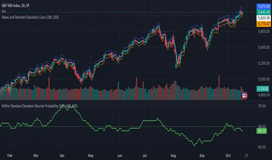
Monthly Price Insights V1 [PINESCRIPTLABS]This indicator displays a chart table that compares the current price of the asset with the closing prices of the last 12 months. This table includes columns for the month, the current price, the previous price, and the percentage change.
Monthly Color Visualization: The indicator uses unique colors for each month, facilitating quick identification of the current and previous periods on the trading chart.
Calculation of Percentage Changes: The indicator calculates the percentage change in price from the previous month, providing a clear perspective on the price trend over time.
Dynamic Data Update: It automatically updates to reflect changes in the asset's price.
Español:
Este indicador muestra una tabla en el gráfico que compara el precio actual del activo con los precios de cierre de los últimos 12 meses. Esta tabla incluye columnas para el mes, el precio actual, el precio anterior y el cambio porcentual.
Visualización por Colores Mensuales: El indicador utiliza colores únicos para cada mes, facilitando la identificación rápida del periodo actual y los anteriores en el gráfico de trading.
Cálculo de Cambios Porcentuales: El indicador calcula el cambio porcentual en el precio desde el mes anterior, proporcionando una perspectiva clara de la tendencia del precio a lo largo del tiempo.
Actualización Dinámica de Datos: Se actualiza automáticamente para reflejar los cambios en el precio del activo.
Pattern Probability with EMA FilterThe provided code is a custom indicator that identifies specific price patterns on a chart and uses a 14-period Exponential Moving Average (EMA) as a filter to display only certain patterns based on the EMA trend direction. These code identifies patterns display them as upward and downward arrows indicates potential price corrections and short term trend reversals in the direction of the arrow. Use with indicators such as RSI that inform overbought and oversold condition to add reliability and confluence.
Code Explanation:
The code first calculates three values 'a', 'b', and 'c' based on the difference between the current high, low, and close prices, respectively, and their respective previous moving average values.
Binary values are then assigned to 'a', 'b', and 'c', where each value is set to 1 if it's greater than 0, and 0 otherwise.
The 'pattern_type' is determined based on the binary values of 'a', 'b', and 'c', combining them into a single number (ranging from 0 to 7) to represent different price patterns.
The code calculates a 14-period Exponential Moving Average (EMA) of the closing price.
It determines the EMA trend direction by comparing the current EMA value with the previous EMA value, setting 'ema_going_up' to true if the EMA is going up and 'ema_going_down' to true if the EMA is going down.
The indicator then plots arrows on the chart for specific pattern_type values while considering the EMA trend direction as a filter. It displays different colored arrows for each pattern_type.
The 14-period EMA is also plotted on the chart, with the color changing to green when the EMA is going up and red when the EMA is going down.
Concept:
pattern_type = 0: H- L- C- (Downward trend continuation) - Indicates a continuation of the downward trend, suggesting further losses ahead.
pattern_type = 1: H- L- C+ (Likely trend change: Downwards to upwards) - Implies the upward trend or price movement change.
pattern_type = 2: H- L+ C- (Likely trend change: Upwards to downwards) - Suggests a potential reversal from an uptrend to a downtrend, but further confirmation is needed.
pattern_type = 3: H- L+ C+ (Trend uncertainty: Potential reversal) - Indicates uncertainty in the trend, potential for a reversal, but further price action confirmation is required.
pattern_type = 4: H+ L- C- (Downward trend continuation with lower volatility) - Suggests the downward trend may continue, but with reduced price swings or lower volatility.
pattern_type = 5: H+ L- C+ (Likely trend change: Downwards to upwards) - Implies a potential reversal from a downtrend to an uptrend, with buying interest increasing.
(pattern_type = 6: H+ L+ C- (Likely trend change: Upwards to downwards) - Suggests a potential reversal from an uptrend to a downtrend, with selling pressure increasing.
pattern_type = 7: H+ L+ C+ (Upward trend continuation) - Indicates a continuation of the upward trend, suggesting further gains ahead.
In the US market, when analyzing a 15-minute chart, we observe the following proportions of the different pattern_type occurrences: The code will plot the low frequency patterns (P1 - P6)
P0 (H- L- C-): 37.60%
P1 (H- L- C+): 3.60%
P2 (H- L+ C-): 3.10%
P3 (H- L+ C+): 3.40%
P4 (H+ L- C-): 2.90%
P5 (H+ L- C+): 2.70%
P6 (H+ L+ C-): 3.50%
P7 (H+ L+ C+): 43.50%
When analyzing higher time frames, such as daily or weekly charts, the occurrence of these patterns is expected to be even lower, but they may carry more significant implications due to their rarity and potential impact on longer-term trends.

SuperTrend Long Strategy +TrendFilterThis strategy aims to identify long (buy) opportunities in the market using the SuperTrend indicator. It utilizes the Average True Range (ATR) and a multiplier to determine the dynamic support levels for entering long positions. This presentation will provide an overview of the strategy's components, explain its usage, and highlight that it focuses on long trades.
Components of the Strategy:
1. ATR Period: This input determines the period used for calculating the Average True Range (ATR). A higher value may result in smoother trend lines but may lag behind recent price changes.
2. Source (src): This input determines the price source used for calculations, with "hl2" (the average of high and low prices) set as the default.
3. ATR Multiplier: This input specifies the multiplier applied to the ATR value to determine the distance of the support levels from the source.
4. Change ATR Calculation Method: This input allows toggling between two methods of ATR calculation: the default method using atr() or a simple moving average (SMA) of ATR values (sma(tr, Periods)).
5. Show Buy/Sell Signals: This input enables or disables the display of buy and sell signals on the chart.
6. Highlighter On/Off: This input controls whether highlighting of up and down trends is displayed on the chart.
7. Bar Coloring On/Off: This input determines whether the bars on the chart are colored based on the trend direction.
8. The "SuperTrend Long STRATEGY" has been enhanced by incorporating a trend filter. A moving average is used as the filter to confirm the prevailing trend before executing trades. This addition effectively reduces false signals and improves the strategy's reliability, all while maintaining its original name.
Strategy Logic:
1. The strategy calculates the upper (up) and lower (dn) trend lines based on the ATR value and the chosen multiplier.
2. The trend variable keeps track of the current trend, with 1 indicating an uptrend and -1 indicating a downtrend.
3. Buy and sell signals are generated based on the change in trend direction.
4. The strategy includes an optional highlighting feature that colors the chart background based on the current trend.
5. Additionally, the bar coloring feature colors the bars based on the direction of the last trend change.
Usage:
1. ATR Period and ATR Multiplier can be adjusted based on the desired sensitivity and risk tolerance.
2. Buy and sell signals can be displayed using the Show Buy/Sell Signals input, providing clear indications of entry and exit points.
3. The Highlighter On/Off input allows users to visually identify the prevailing trend by coloring the chart background.
4. The Bar Coloring On/Off input offers a quick visual reference for the most recent trend change.
Long Strategy:
The SuperTrend Long Strategy is specifically designed to identify long (buy) opportunities. It generates buy signals when the current trend changes from a downtrend to an uptrend, indicating a potential entry point for long positions. The strategy aims to capture upward price movements and maximize profits during bullish market conditions.
The SuperTrend Long Strategy provides traders with a systematic approach to identifying long trade opportunities. By leveraging the SuperTrend indicator and dynamic support levels, this strategy aims to generate buy signals in uptrending markets. Traders can customize the inputs and utilize the visual features to adapt the strategy to their specific trading preferences.
The modification adds a trend filter to the "SuperTrend Long STRATEGY" to improve its effectiveness. The trend filter uses a moving average to confirm the prevailing trend before taking trades. This addition helps filter out false signals and enhances the strategy's reliability without changing its name.

Goertzel Browser [Loxx]As the financial markets become increasingly complex and data-driven, traders and analysts must leverage powerful tools to gain insights and make informed decisions. One such tool is the Goertzel Browser indicator, a sophisticated technical analysis indicator that helps identify cyclical patterns in financial data. This powerful tool is capable of detecting cyclical patterns in financial data, helping traders to make better predictions and optimize their trading strategies. With its unique combination of mathematical algorithms and advanced charting capabilities, this indicator has the potential to revolutionize the way we approach financial modeling and trading.
█ Brief Overview of the Goertzel Browser
The Goertzel Browser is a sophisticated technical analysis tool that utilizes the Goertzel algorithm to analyze and visualize cyclical components within a financial time series. By identifying these cycles and their characteristics, the indicator aims to provide valuable insights into the market's underlying price movements, which could potentially be used for making informed trading decisions.
The primary purpose of this indicator is to:
1. Detect and analyze the dominant cycles present in the price data.
2. Reconstruct and visualize the composite wave based on the detected cycles.
3. Project the composite wave into the future, providing a potential roadmap for upcoming price movements.
To achieve this, the indicator performs several tasks:
1. Detrending the price data: The indicator preprocesses the price data using various detrending techniques, such as Hodrick-Prescott filters, zero-lag moving averages, and linear regression, to remove the underlying trend and focus on the cyclical components.
2. Applying the Goertzel algorithm: The indicator applies the Goertzel algorithm to the detrended price data, identifying the dominant cycles and their characteristics, such as amplitude, phase, and cycle strength.
3. Constructing the composite wave: The indicator reconstructs the composite wave by combining the detected cycles, either by using a user-defined list of cycles or by selecting the top N cycles based on their amplitude or cycle strength.
4. Visualizing the composite wave: The indicator plots the composite wave, using solid lines for the past and dotted lines for the future projections. The color of the lines indicates whether the wave is increasing or decreasing.
5. Displaying cycle information: The indicator provides a table that displays detailed information about the detected cycles, including their rank, period, Bartel's test results, amplitude, and phase.
This indicator is a powerful tool that employs the Goertzel algorithm to analyze and visualize the cyclical components within a financial time series. By providing insights into the underlying price movements and their potential future trajectory, the indicator aims to assist traders in making more informed decisions.
█ What is the Goertzel Algorithm?
The Goertzel algorithm, named after Gerald Goertzel, is a digital signal processing technique that is used to efficiently compute individual terms of the Discrete Fourier Transform (DFT). It was first introduced in 1958, and since then, it has found various applications in the fields of engineering, mathematics, and physics.
The Goertzel algorithm is primarily used to detect specific frequency components within a digital signal, making it particularly useful in applications where only a few frequency components are of interest. The algorithm is computationally efficient, as it requires fewer calculations than the Fast Fourier Transform (FFT) when detecting a small number of frequency components. This efficiency makes the Goertzel algorithm a popular choice in applications such as:
1. Telecommunications: The Goertzel algorithm is used for decoding Dual-Tone Multi-Frequency (DTMF) signals, which are the tones generated when pressing buttons on a telephone keypad. By identifying specific frequency components, the algorithm can accurately determine which button has been pressed.
2. Audio processing: The algorithm can be used to detect specific pitches or harmonics in an audio signal, making it useful in applications like pitch detection and tuning musical instruments.
3. Vibration analysis: In the field of mechanical engineering, the Goertzel algorithm can be applied to analyze vibrations in rotating machinery, helping to identify faulty components or signs of wear.
4. Power system analysis: The algorithm can be used to measure harmonic content in power systems, allowing engineers to assess power quality and detect potential issues.
The Goertzel algorithm is used in these applications because it offers several advantages over other methods, such as the FFT:
1. Computational efficiency: The Goertzel algorithm requires fewer calculations when detecting a small number of frequency components, making it more computationally efficient than the FFT in these cases.
2. Real-time analysis: The algorithm can be implemented in a streaming fashion, allowing for real-time analysis of signals, which is crucial in applications like telecommunications and audio processing.
3. Memory efficiency: The Goertzel algorithm requires less memory than the FFT, as it only computes the frequency components of interest.
4. Precision: The algorithm is less susceptible to numerical errors compared to the FFT, ensuring more accurate results in applications where precision is essential.
The Goertzel algorithm is an efficient digital signal processing technique that is primarily used to detect specific frequency components within a signal. Its computational efficiency, real-time capabilities, and precision make it an attractive choice for various applications, including telecommunications, audio processing, vibration analysis, and power system analysis. The algorithm has been widely adopted since its introduction in 1958 and continues to be an essential tool in the fields of engineering, mathematics, and physics.
█ Goertzel Algorithm in Quantitative Finance: In-Depth Analysis and Applications
The Goertzel algorithm, initially designed for signal processing in telecommunications, has gained significant traction in the financial industry due to its efficient frequency detection capabilities. In quantitative finance, the Goertzel algorithm has been utilized for uncovering hidden market cycles, developing data-driven trading strategies, and optimizing risk management. This section delves deeper into the applications of the Goertzel algorithm in finance, particularly within the context of quantitative trading and analysis.
Unveiling Hidden Market Cycles:
Market cycles are prevalent in financial markets and arise from various factors, such as economic conditions, investor psychology, and market participant behavior. The Goertzel algorithm's ability to detect and isolate specific frequencies in price data helps trader analysts identify hidden market cycles that may otherwise go unnoticed. By examining the amplitude, phase, and periodicity of each cycle, traders can better understand the underlying market structure and dynamics, enabling them to develop more informed and effective trading strategies.
Developing Quantitative Trading Strategies:
The Goertzel algorithm's versatility allows traders to incorporate its insights into a wide range of trading strategies. By identifying the dominant market cycles in a financial instrument's price data, traders can create data-driven strategies that capitalize on the cyclical nature of markets.
For instance, a trader may develop a mean-reversion strategy that takes advantage of the identified cycles. By establishing positions when the price deviates from the predicted cycle, the trader can profit from the subsequent reversion to the cycle's mean. Similarly, a momentum-based strategy could be designed to exploit the persistence of a dominant cycle by entering positions that align with the cycle's direction.
Enhancing Risk Management:
The Goertzel algorithm plays a vital role in risk management for quantitative strategies. By analyzing the cyclical components of a financial instrument's price data, traders can gain insights into the potential risks associated with their trading strategies.
By monitoring the amplitude and phase of dominant cycles, a trader can detect changes in market dynamics that may pose risks to their positions. For example, a sudden increase in amplitude may indicate heightened volatility, prompting the trader to adjust position sizing or employ hedging techniques to protect their portfolio. Additionally, changes in phase alignment could signal a potential shift in market sentiment, necessitating adjustments to the trading strategy.
Expanding Quantitative Toolkits:
Traders can augment the Goertzel algorithm's insights by combining it with other quantitative techniques, creating a more comprehensive and sophisticated analysis framework. For example, machine learning algorithms, such as neural networks or support vector machines, could be trained on features extracted from the Goertzel algorithm to predict future price movements more accurately.
Furthermore, the Goertzel algorithm can be integrated with other technical analysis tools, such as moving averages or oscillators, to enhance their effectiveness. By applying these tools to the identified cycles, traders can generate more robust and reliable trading signals.
The Goertzel algorithm offers invaluable benefits to quantitative finance practitioners by uncovering hidden market cycles, aiding in the development of data-driven trading strategies, and improving risk management. By leveraging the insights provided by the Goertzel algorithm and integrating it with other quantitative techniques, traders can gain a deeper understanding of market dynamics and devise more effective trading strategies.
█ Indicator Inputs
src: This is the source data for the analysis, typically the closing price of the financial instrument.
detrendornot: This input determines the method used for detrending the source data. Detrending is the process of removing the underlying trend from the data to focus on the cyclical components.
The available options are:
hpsmthdt: Detrend using Hodrick-Prescott filter centered moving average.
zlagsmthdt: Detrend using zero-lag moving average centered moving average.
logZlagRegression: Detrend using logarithmic zero-lag linear regression.
hpsmth: Detrend using Hodrick-Prescott filter.
zlagsmth: Detrend using zero-lag moving average.
DT_HPper1 and DT_HPper2: These inputs define the period range for the Hodrick-Prescott filter centered moving average when detrendornot is set to hpsmthdt.
DT_ZLper1 and DT_ZLper2: These inputs define the period range for the zero-lag moving average centered moving average when detrendornot is set to zlagsmthdt.
DT_RegZLsmoothPer: This input defines the period for the zero-lag moving average used in logarithmic zero-lag linear regression when detrendornot is set to logZlagRegression.
HPsmoothPer: This input defines the period for the Hodrick-Prescott filter when detrendornot is set to hpsmth.
ZLMAsmoothPer: This input defines the period for the zero-lag moving average when detrendornot is set to zlagsmth.
MaxPer: This input sets the maximum period for the Goertzel algorithm to search for cycles.
squaredAmp: This boolean input determines whether the amplitude should be squared in the Goertzel algorithm.
useAddition: This boolean input determines whether the Goertzel algorithm should use addition for combining the cycles.
useCosine: This boolean input determines whether the Goertzel algorithm should use cosine waves instead of sine waves.
UseCycleStrength: This boolean input determines whether the Goertzel algorithm should compute the cycle strength, which is a normalized measure of the cycle's amplitude.
WindowSizePast and WindowSizeFuture: These inputs define the window size for past and future projections of the composite wave.
FilterBartels: This boolean input determines whether Bartel's test should be applied to filter out non-significant cycles.
BartNoCycles: This input sets the number of cycles to be used in Bartel's test.
BartSmoothPer: This input sets the period for the moving average used in Bartel's test.
BartSigLimit: This input sets the significance limit for Bartel's test, below which cycles are considered insignificant.
SortBartels: This boolean input determines whether the cycles should be sorted by their Bartel's test results.
UseCycleList: This boolean input determines whether a user-defined list of cycles should be used for constructing the composite wave. If set to false, the top N cycles will be used.
Cycle1, Cycle2, Cycle3, Cycle4, and Cycle5: These inputs define the user-defined list of cycles when 'UseCycleList' is set to true. If using a user-defined list, each of these inputs represents the period of a specific cycle to include in the composite wave.
StartAtCycle: This input determines the starting index for selecting the top N cycles when UseCycleList is set to false. This allows you to skip a certain number of cycles from the top before selecting the desired number of cycles.
UseTopCycles: This input sets the number of top cycles to use for constructing the composite wave when UseCycleList is set to false. The cycles are ranked based on their amplitudes or cycle strengths, depending on the UseCycleStrength input.
SubtractNoise: This boolean input determines whether to subtract the noise (remaining cycles) from the composite wave. If set to true, the composite wave will only include the top N cycles specified by UseTopCycles.
█ Exploring Auxiliary Functions
The following functions demonstrate advanced techniques for analyzing financial markets, including zero-lag moving averages, Bartels probability, detrending, and Hodrick-Prescott filtering. This section examines each function in detail, explaining their purpose, methodology, and applications in finance. We will examine how each function contributes to the overall performance and effectiveness of the indicator and how they work together to create a powerful analytical tool.
Zero-Lag Moving Average:
The zero-lag moving average function is designed to minimize the lag typically associated with moving averages. This is achieved through a two-step weighted linear regression process that emphasizes more recent data points. The function calculates a linearly weighted moving average (LWMA) on the input data and then applies another LWMA on the result. By doing this, the function creates a moving average that closely follows the price action, reducing the lag and improving the responsiveness of the indicator.
The zero-lag moving average function is used in the indicator to provide a responsive, low-lag smoothing of the input data. This function helps reduce the noise and fluctuations in the data, making it easier to identify and analyze underlying trends and patterns. By minimizing the lag associated with traditional moving averages, this function allows the indicator to react more quickly to changes in market conditions, providing timely signals and improving the overall effectiveness of the indicator.
Bartels Probability:
The Bartels probability function calculates the probability of a given cycle being significant in a time series. It uses a mathematical test called the Bartels test to assess the significance of cycles detected in the data. The function calculates coefficients for each detected cycle and computes an average amplitude and an expected amplitude. By comparing these values, the Bartels probability is derived, indicating the likelihood of a cycle's significance. This information can help in identifying and analyzing dominant cycles in financial markets.
The Bartels probability function is incorporated into the indicator to assess the significance of detected cycles in the input data. By calculating the Bartels probability for each cycle, the indicator can prioritize the most significant cycles and focus on the market dynamics that are most relevant to the current trading environment. This function enhances the indicator's ability to identify dominant market cycles, improving its predictive power and aiding in the development of effective trading strategies.
Detrend Logarithmic Zero-Lag Regression:
The detrend logarithmic zero-lag regression function is used for detrending data while minimizing lag. It combines a zero-lag moving average with a linear regression detrending method. The function first calculates the zero-lag moving average of the logarithm of input data and then applies a linear regression to remove the trend. By detrending the data, the function isolates the cyclical components, making it easier to analyze and interpret the underlying market dynamics.
The detrend logarithmic zero-lag regression function is used in the indicator to isolate the cyclical components of the input data. By detrending the data, the function enables the indicator to focus on the cyclical movements in the market, making it easier to analyze and interpret market dynamics. This function is essential for identifying cyclical patterns and understanding the interactions between different market cycles, which can inform trading decisions and enhance overall market understanding.
Bartels Cycle Significance Test:
The Bartels cycle significance test is a function that combines the Bartels probability function and the detrend logarithmic zero-lag regression function to assess the significance of detected cycles. The function calculates the Bartels probability for each cycle and stores the results in an array. By analyzing the probability values, traders and analysts can identify the most significant cycles in the data, which can be used to develop trading strategies and improve market understanding.
The Bartels cycle significance test function is integrated into the indicator to provide a comprehensive analysis of the significance of detected cycles. By combining the Bartels probability function and the detrend logarithmic zero-lag regression function, this test evaluates the significance of each cycle and stores the results in an array. The indicator can then use this information to prioritize the most significant cycles and focus on the most relevant market dynamics. This function enhances the indicator's ability to identify and analyze dominant market cycles, providing valuable insights for trading and market analysis.
Hodrick-Prescott Filter:
The Hodrick-Prescott filter is a popular technique used to separate the trend and cyclical components of a time series. The function applies a smoothing parameter to the input data and calculates a smoothed series using a two-sided filter. This smoothed series represents the trend component, which can be subtracted from the original data to obtain the cyclical component. The Hodrick-Prescott filter is commonly used in economics and finance to analyze economic data and financial market trends.
The Hodrick-Prescott filter is incorporated into the indicator to separate the trend and cyclical components of the input data. By applying the filter to the data, the indicator can isolate the trend component, which can be used to analyze long-term market trends and inform trading decisions. Additionally, the cyclical component can be used to identify shorter-term market dynamics and provide insights into potential trading opportunities. The inclusion of the Hodrick-Prescott filter adds another layer of analysis to the indicator, making it more versatile and comprehensive.
Detrending Options: Detrend Centered Moving Average:
The detrend centered moving average function provides different detrending methods, including the Hodrick-Prescott filter and the zero-lag moving average, based on the selected detrending method. The function calculates two sets of smoothed values using the chosen method and subtracts one set from the other to obtain a detrended series. By offering multiple detrending options, this function allows traders and analysts to select the most appropriate method for their specific needs and preferences.
The detrend centered moving average function is integrated into the indicator to provide users with multiple detrending options, including the Hodrick-Prescott filter and the zero-lag moving average. By offering multiple detrending methods, the indicator allows users to customize the analysis to their specific needs and preferences, enhancing the indicator's overall utility and adaptability. This function ensures that the indicator can cater to a wide range of trading styles and objectives, making it a valuable tool for a diverse group of market participants.
The auxiliary functions functions discussed in this section demonstrate the power and versatility of mathematical techniques in analyzing financial markets. By understanding and implementing these functions, traders and analysts can gain valuable insights into market dynamics, improve their trading strategies, and make more informed decisions. The combination of zero-lag moving averages, Bartels probability, detrending methods, and the Hodrick-Prescott filter provides a comprehensive toolkit for analyzing and interpreting financial data. The integration of advanced functions in a financial indicator creates a powerful and versatile analytical tool that can provide valuable insights into financial markets. By combining the zero-lag moving average,
█ In-Depth Analysis of the Goertzel Browser Code
The Goertzel Browser code is an implementation of the Goertzel Algorithm, an efficient technique to perform spectral analysis on a signal. The code is designed to detect and analyze dominant cycles within a given financial market data set. This section will provide an extremely detailed explanation of the code, its structure, functions, and intended purpose.
Function signature and input parameters:
The Goertzel Browser function accepts numerous input parameters for customization, including source data (src), the current bar (forBar), sample size (samplesize), period (per), squared amplitude flag (squaredAmp), addition flag (useAddition), cosine flag (useCosine), cycle strength flag (UseCycleStrength), past and future window sizes (WindowSizePast, WindowSizeFuture), Bartels filter flag (FilterBartels), Bartels-related parameters (BartNoCycles, BartSmoothPer, BartSigLimit), sorting flag (SortBartels), and output buffers (goeWorkPast, goeWorkFuture, cyclebuffer, amplitudebuffer, phasebuffer, cycleBartelsBuffer).
Initializing variables and arrays:
The code initializes several float arrays (goeWork1, goeWork2, goeWork3, goeWork4) with the same length as twice the period (2 * per). These arrays store intermediate results during the execution of the algorithm.
Preprocessing input data:
The input data (src) undergoes preprocessing to remove linear trends. This step enhances the algorithm's ability to focus on cyclical components in the data. The linear trend is calculated by finding the slope between the first and last values of the input data within the sample.
Iterative calculation of Goertzel coefficients:
The core of the Goertzel Browser algorithm lies in the iterative calculation of Goertzel coefficients for each frequency bin. These coefficients represent the spectral content of the input data at different frequencies. The code iterates through the range of frequencies, calculating the Goertzel coefficients using a nested loop structure.
Cycle strength computation:
The code calculates the cycle strength based on the Goertzel coefficients. This is an optional step, controlled by the UseCycleStrength flag. The cycle strength provides information on the relative influence of each cycle on the data per bar, considering both amplitude and cycle length. The algorithm computes the cycle strength either by squaring the amplitude (controlled by squaredAmp flag) or using the actual amplitude values.
Phase calculation:
The Goertzel Browser code computes the phase of each cycle, which represents the position of the cycle within the input data. The phase is calculated using the arctangent function (math.atan) based on the ratio of the imaginary and real components of the Goertzel coefficients.
Peak detection and cycle extraction:
The algorithm performs peak detection on the computed amplitudes or cycle strengths to identify dominant cycles. It stores the detected cycles in the cyclebuffer array, along with their corresponding amplitudes and phases in the amplitudebuffer and phasebuffer arrays, respectively.
Sorting cycles by amplitude or cycle strength:
The code sorts the detected cycles based on their amplitude or cycle strength in descending order. This allows the algorithm to prioritize cycles with the most significant impact on the input data.
Bartels cycle significance test:
If the FilterBartels flag is set, the code performs a Bartels cycle significance test on the detected cycles. This test determines the statistical significance of each cycle and filters out the insignificant cycles. The significant cycles are stored in the cycleBartelsBuffer array. If the SortBartels flag is set, the code sorts the significant cycles based on their Bartels significance values.
Waveform calculation:
The Goertzel Browser code calculates the waveform of the significant cycles for both past and future time windows. The past and future windows are defined by the WindowSizePast and WindowSizeFuture parameters, respectively. The algorithm uses either cosine or sine functions (controlled by the useCosine flag) to calculate the waveforms for each cycle. The useAddition flag determines whether the waveforms should be added or subtracted.
Storing waveforms in matrices:
The calculated waveforms for each cycle are stored in two matrices - goeWorkPast and goeWorkFuture. These matrices hold the waveforms for the past and future time windows, respectively. Each row in the matrices represents a time window position, and each column corresponds to a cycle.
Returning the number of cycles:
The Goertzel Browser function returns the total number of detected cycles (number_of_cycles) after processing the input data. This information can be used to further analyze the results or to visualize the detected cycles.
The Goertzel Browser code is a comprehensive implementation of the Goertzel Algorithm, specifically designed for detecting and analyzing dominant cycles within financial market data. The code offers a high level of customization, allowing users to fine-tune the algorithm based on their specific needs. The Goertzel Browser's combination of preprocessing, iterative calculations, cycle extraction, sorting, significance testing, and waveform calculation makes it a powerful tool for understanding cyclical components in financial data.
█ Generating and Visualizing Composite Waveform
The indicator calculates and visualizes the composite waveform for both past and future time windows based on the detected cycles. Here's a detailed explanation of this process:
Updating WindowSizePast and WindowSizeFuture:
The WindowSizePast and WindowSizeFuture are updated to ensure they are at least twice the MaxPer (maximum period).
Initializing matrices and arrays:
Two matrices, goeWorkPast and goeWorkFuture, are initialized to store the Goertzel results for past and future time windows. Multiple arrays are also initialized to store cycle, amplitude, phase, and Bartels information.
Preparing the source data (srcVal) array:
The source data is copied into an array, srcVal, and detrended using one of the selected methods (hpsmthdt, zlagsmthdt, logZlagRegression, hpsmth, or zlagsmth).
Goertzel function call:
The Goertzel function is called to analyze the detrended source data and extract cycle information. The output, number_of_cycles, contains the number of detected cycles.
Initializing arrays for past and future waveforms:
Three arrays, epgoertzel, goertzel, and goertzelFuture, are initialized to store the endpoint Goertzel, non-endpoint Goertzel, and future Goertzel projections, respectively.
Calculating composite waveform for past bars (goertzel array):
The past composite waveform is calculated by summing the selected cycles (either from the user-defined cycle list or the top cycles) and optionally subtracting the noise component.
Calculating composite waveform for future bars (goertzelFuture array):
The future composite waveform is calculated in a similar way as the past composite waveform.
Drawing past composite waveform (pvlines):
The past composite waveform is drawn on the chart using solid lines. The color of the lines is determined by the direction of the waveform (green for upward, red for downward).
Drawing future composite waveform (fvlines):
The future composite waveform is drawn on the chart using dotted lines. The color of the lines is determined by the direction of the waveform (fuchsia for upward, yellow for downward).
Displaying cycle information in a table (table3):
A table is created to display the cycle information, including the rank, period, Bartel value, amplitude (or cycle strength), and phase of each detected cycle.
Filling the table with cycle information:
The indicator iterates through the detected cycles and retrieves the relevant information (period, amplitude, phase, and Bartel value) from the corresponding arrays. It then fills the table with this information, displaying the values up to six decimal places.
To summarize, this indicator generates a composite waveform based on the detected cycles in the financial data. It calculates the composite waveforms for both past and future time windows and visualizes them on the chart using colored lines. Additionally, it displays detailed cycle information in a table, including the rank, period, Bartel value, amplitude (or cycle strength), and phase of each detected cycle.
█ Enhancing the Goertzel Algorithm-Based Script for Financial Modeling and Trading
The Goertzel algorithm-based script for detecting dominant cycles in financial data is a powerful tool for financial modeling and trading. It provides valuable insights into the past behavior of these cycles and potential future impact. However, as with any algorithm, there is always room for improvement. This section discusses potential enhancements to the existing script to make it even more robust and versatile for financial modeling, general trading, advanced trading, and high-frequency finance trading.
Enhancements for Financial Modeling
Data preprocessing: One way to improve the script's performance for financial modeling is to introduce more advanced data preprocessing techniques. This could include removing outliers, handling missing data, and normalizing the data to ensure consistent and accurate results.
Additional detrending and smoothing methods: Incorporating more sophisticated detrending and smoothing techniques, such as wavelet transform or empirical mode decomposition, can help improve the script's ability to accurately identify cycles and trends in the data.
Machine learning integration: Integrating machine learning techniques, such as artificial neural networks or support vector machines, can help enhance the script's predictive capabilities, leading to more accurate financial models.
Enhancements for General and Advanced Trading
Customizable indicator integration: Allowing users to integrate their own technical indicators can help improve the script's effectiveness for both general and advanced trading. By enabling the combination of the dominant cycle information with other technical analysis tools, traders can develop more comprehensive trading strategies.
Risk management and position sizing: Incorporating risk management and position sizing functionality into the script can help traders better manage their trades and control potential losses. This can be achieved by calculating the optimal position size based on the user's risk tolerance and account size.
Multi-timeframe analysis: Enhancing the script to perform multi-timeframe analysis can provide traders with a more holistic view of market trends and cycles. By identifying dominant cycles on different timeframes, traders can gain insights into the potential confluence of cycles and make better-informed trading decisions.
Enhancements for High-Frequency Finance Trading
Algorithm optimization: To ensure the script's suitability for high-frequency finance trading, optimizing the algorithm for faster execution is crucial. This can be achieved by employing efficient data structures and refining the calculation methods to minimize computational complexity.
Real-time data streaming: Integrating real-time data streaming capabilities into the script can help high-frequency traders react to market changes more quickly. By continuously updating the cycle information based on real-time market data, traders can adapt their strategies accordingly and capitalize on short-term market fluctuations.
Order execution and trade management: To fully leverage the script's capabilities for high-frequency trading, implementing functionality for automated order execution and trade management is essential. This can include features such as stop-loss and take-profit orders, trailing stops, and automated trade exit strategies.
While the existing Goertzel algorithm-based script is a valuable tool for detecting dominant cycles in financial data, there are several potential enhancements that can make it even more powerful for financial modeling, general trading, advanced trading, and high-frequency finance trading. By incorporating these improvements, the script can become a more versatile and effective tool for traders and financial analysts alike.
█ Understanding the Limitations of the Goertzel Algorithm
While the Goertzel algorithm-based script for detecting dominant cycles in financial data provides valuable insights, it is important to be aware of its limitations and drawbacks. Some of the key drawbacks of this indicator are:
Lagging nature:
As with many other technical indicators, the Goertzel algorithm-based script can suffer from lagging effects, meaning that it may not immediately react to real-time market changes. This lag can lead to late entries and exits, potentially resulting in reduced profitability or increased losses.
Parameter sensitivity:
The performance of the script can be sensitive to the chosen parameters, such as the detrending methods, smoothing techniques, and cycle detection settings. Improper parameter selection may lead to inaccurate cycle detection or increased false signals, which can negatively impact trading performance.
Complexity:
The Goertzel algorithm itself is relatively complex, making it difficult for novice traders or those unfamiliar with the concept of cycle analysis to fully understand and effectively utilize the script. This complexity can also make it challenging to optimize the script for specific trading styles or market conditions.
Overfitting risk:
As with any data-driven approach, there is a risk of overfitting when using the Goertzel algorithm-based script. Overfitting occurs when a model becomes too specific to the historical data it was trained on, leading to poor performance on new, unseen data. This can result in misleading signals and reduced trading performance.
No guarantee of future performance: While the script can provide insights into past cycles and potential future trends, it is important to remember that past performance does not guarantee future results. Market conditions can change, and relying solely on the script's predictions without considering other factors may lead to poor trading decisions.
Limited applicability: The Goertzel algorithm-based script may not be suitable for all markets, trading styles, or timeframes. Its effectiveness in detecting cycles may be limited in certain market conditions, such as during periods of extreme volatility or low liquidity.
While the Goertzel algorithm-based script offers valuable insights into dominant cycles in financial data, it is essential to consider its drawbacks and limitations when incorporating it into a trading strategy. Traders should always use the script in conjunction with other technical and fundamental analysis tools, as well as proper risk management, to make well-informed trading decisions.
█ Interpreting Results
The Goertzel Browser indicator can be interpreted by analyzing the plotted lines and the table presented alongside them. The indicator plots two lines: past and future composite waves. The past composite wave represents the composite wave of the past price data, and the future composite wave represents the projected composite wave for the next period.
The past composite wave line displays a solid line, with green indicating a bullish trend and red indicating a bearish trend. On the other hand, the future composite wave line is a dotted line with fuchsia indicating a bullish trend and yellow indicating a bearish trend.
The table presented alongside the indicator shows the top cycles with their corresponding rank, period, Bartels, amplitude or cycle strength, and phase. The amplitude is a measure of the strength of the cycle, while the phase is the position of the cycle within the data series.
Interpreting the Goertzel Browser indicator involves identifying the trend of the past and future composite wave lines and matching them with the corresponding bullish or bearish color. Additionally, traders can identify the top cycles with the highest amplitude or cycle strength and utilize them in conjunction with other technical indicators and fundamental analysis for trading decisions.
This indicator is considered a repainting indicator because the value of the indicator is calculated based on the past price data. As new price data becomes available, the indicator's value is recalculated, potentially causing the indicator's past values to change. This can create a false impression of the indicator's performance, as it may appear to have provided a profitable trading signal in the past when, in fact, that signal did not exist at the time.
The Goertzel indicator is also non-endpointed, meaning that it is not calculated up to the current bar or candle. Instead, it uses a fixed amount of historical data to calculate its values, which can make it difficult to use for real-time trading decisions. For example, if the indicator uses 100 bars of historical data to make its calculations, it cannot provide a signal until the current bar has closed and become part of the historical data. This can result in missed trading opportunities or delayed signals.
█ Conclusion
The Goertzel Browser indicator is a powerful tool for identifying and analyzing cyclical patterns in financial markets. Its ability to detect multiple cycles of varying frequencies and strengths make it a valuable addition to any trader's technical analysis toolkit. However, it is important to keep in mind that the Goertzel Browser indicator should be used in conjunction with other technical analysis tools and fundamental analysis to achieve the best results. With continued refinement and development, the Goertzel Browser indicator has the potential to become a highly effective tool for financial modeling, general trading, advanced trading, and high-frequency finance trading. Its accuracy and versatility make it a promising candidate for further research and development.
█ Footnotes
What is the Bartels Test for Cycle Significance?
The Bartels Cycle Significance Test is a statistical method that determines whether the peaks and troughs of a time series are statistically significant. The test is named after its inventor, George Bartels, who developed it in the mid-20th century.
The Bartels test is designed to analyze the cyclical components of a time series, which can help traders and analysts identify trends and cycles in financial markets. The test calculates a Bartels statistic, which measures the degree of non-randomness or autocorrelation in the time series.
The Bartels statistic is calculated by first splitting the time series into two halves and calculating the range of the peaks and troughs in each half. The test then compares these ranges using a t-test, which measures the significance of the difference between the two ranges.
If the Bartels statistic is greater than a critical value, it indicates that the peaks and troughs in the time series are non-random and that there is a significant cyclical component to the data. Conversely, if the Bartels statistic is less than the critical value, it suggests that the peaks and troughs are random and that there is no significant cyclical component.
The Bartels Cycle Significance Test is particularly useful in financial analysis because it can help traders and analysts identify significant cycles in asset prices, which can in turn inform investment decisions. However, it is important to note that the test is not perfect and can produce false signals in certain situations, particularly in noisy or volatile markets. Therefore, it is always recommended to use the test in conjunction with other technical and fundamental indicators to confirm trends and cycles.
Deep-dive into the Hodrick-Prescott Fitler
The Hodrick-Prescott (HP) filter is a statistical tool used in economics and finance to separate a time series into two components: a trend component and a cyclical component. It is a powerful tool for identifying long-term trends in economic and financial data and is widely used by economists, central banks, and financial institutions around the world.
The HP filter was first introduced in the 1990s by economists Robert Hodrick and Edward Prescott. It is a simple, two-parameter filter that separates a time series into a trend component and a cyclical component. The trend component represents the long-term behavior of the data, while the cyclical component captures the shorter-term fluctuations around the trend.
The HP filter works by minimizing the following objective function:
Minimize: (Sum of Squared Deviations) + λ (Sum of Squared Second Differences)
Where:
The first term represents the deviation of the data from the trend.
The second term represents the smoothness of the trend.
λ is a smoothing parameter that determines the degree of smoothness of the trend.
The smoothing parameter λ is typically set to a value between 100 and 1600, depending on the frequency of the data. Higher values of λ lead to a smoother trend, while lower values lead to a more volatile trend.
The HP filter has several advantages over other smoothing techniques. It is a non-parametric method, meaning that it does not make any assumptions about the underlying distribution of the data. It also allows for easy comparison of trends across different time series and can be used with data of any frequency.
However, the HP filter also has some limitations. It assumes that the trend is a smooth function, which may not be the case in some situations. It can also be sensitive to changes in the smoothing parameter λ, which may result in different trends for the same data. Additionally, the filter may produce unrealistic trends for very short time series.
Despite these limitations, the HP filter remains a valuable tool for analyzing economic and financial data. It is widely used by central banks and financial institutions to monitor long-term trends in the economy, and it can be used to identify turning points in the business cycle. The filter can also be used to analyze asset prices, exchange rates, and other financial variables.
The Hodrick-Prescott filter is a powerful tool for analyzing economic and financial data. It separates a time series into a trend component and a cyclical component, allowing for easy identification of long-term trends and turning points in the business cycle. While it has some limitations, it remains a valuable tool for economists, central banks, and financial institutions around the world.

Big 8 Intraday TICKAt the start of each trading day (0930 EST), this indicator calculates the intraday price difference between open and close for the eight largest market cap stocks (AAPL, AMZN, GOOGLE, META, MSFT, NFLX, NVDA, and TSLA), assigns a +/-1 for each, and then plots the cumulative change. An EMA has been added for smoothing purposes that is set to 5 but can be changed. Please note indicator is best used on lower timeframes (15 min or less) and has no applicability to time frames above 1 hour.
The thought behind this indicator is those eight major stocks drive a majority of intraday price change in indices like SPY and QQQ that are heavily weighted towards these stocks, therefore they should be a leading indicator in price change. You can often catch a move in SPY or QQQ one to two bars (on 1 min chart) ahead of the actual move because you see this indicator moving strong to one direction.
It's not perfect as there are divergences you will see when you compare historical charts, but oftentimes those divergences ultimately lead to significant price swings in the same direction as this indicator, so recommend being on watch to pull the trigger when you see those and price confirms.
You can use this indicator in a few ways:
1. Confirmation that your current trade is in the same direction as this indicator
2. Use the zero cross as a trigger for put or call entry
3. Focusing only on calls/longs if the value is above 0, or only puts/shorts if the value is below zero. Just be sure to keep an eye on reversals.
If you have recommendations on how to improve, let me know and I'll do my best to make changes.

Open Close Cross Strategy R6.1 revised by yourmattieOriginal version: Open Close Cross Strategy R5 revised by JustUncle.
Change: script changed to a study script with custom alerts.
This revision is an open Public release, with just some minor changes. It is a revision of the Strategy "Open Close Cross Strategy R2" originally published by @JayRogers.
Revised by JustUncleL
Description :
Strategy based around Open-Close Moving Average Crossovers optionally from a higher time frame.
Read more about the indicator original script
Klik here
##USE AT YOUR OWN RISK##
Use this as overlayer on the original strategy to set custom alerts.
Info: with this study script no buy/sell arrows show up op the chart.
Does some know a solution for this issue:
Issue: sometimes it gives a false signal because even when you set "one per bar close" the custom set alert might come halfway the bar....and it might be a false signal when the bar is closed
Does somone know a fix for this? I tried with barstate.iscomfirmed but it didn't work for me.
Ps. I'm not a developer...just changed the scipt by watching a youtube tutorial.
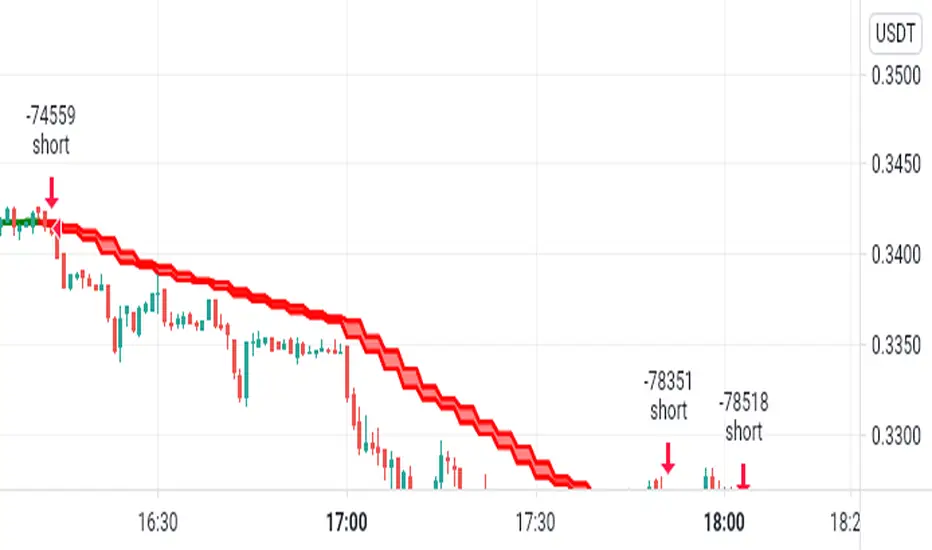
Multi-Timeframe Supertrend + MACD + MTF Dashboard if you like it click source code and save it in notepad for back up .
The Multi-Timeframe Supertrend Dashboard is a powerful tool designed to give traders a clear view of market trends across multiple timeframes, all from a single dashboard. This indicator leverages the Supertrend method to calculate buy and sell signals based on the direction of price relative to dynamically calculated support and resistance lines. The dashboard is optimized for dark mode and provides easy-to-interpret color-coded signals for each timeframe.
How It Works
The Supertrend indicator is a trend-following indicator that uses the Average True Range (ATR) to set upper and lower bands around the price, adapting dynamically as volatility changes. When the price is above the Supertrend line, the market is considered in an uptrend, triggering a "BUY" signal. Conversely, when the price falls below the Supertrend line, the market is in a downtrend, triggering a "SELL" signal.
This Multi-Timeframe Supertrend Dashboard calculates Supertrend signals for the following timeframes:
1 minute
5 minutes
15 minutes
1 hour
Daily
Weekly
Monthly
For each timeframe, the dashboard shows either a "BUY" or "SELL" signal, allowing traders to assess whether trends align across timeframes. A "BUY" signal displays in green, and a "SELL" signal displays in red, giving a quick visual reference of the overall trend direction for each timeframe.
Customization Options
ATR Period: Defines the period for the Average True Range (ATR) calculation, which determines how responsive the Supertrend lines are to changes in market volatility.
Multiplier: Sets the sensitivity of the Supertrend bands to price movements. Higher values make the bands less sensitive, while lower values increase sensitivity, allowing quicker reactions to changes in price.
How to Interpret the Dashboard
The Multi-Timeframe Supertrend Dashboard allows traders to see at a glance if trends across multiple timeframes are aligned. Here’s how to interpret the signals:
BUY (Green): The current timeframe’s price is in an uptrend based on the Supertrend calculation.
SELL (Red): The current timeframe’s price is in a downtrend based on the Supertrend calculation.
For example:
If all timeframes display "BUY," the asset is in a strong uptrend across multiple time horizons, which may indicate a bullish market.
If all timeframes display "SELL," the asset is likely in a strong downtrend, signaling a bearish market.
Mixed signals across timeframes suggest market consolidation or differing trends across short- and long-term periods.
Use Cases
Trend Confirmation: Use the dashboard to confirm trends across multiple timeframes before entering or exiting a position.
Quick Market Analysis: Get a snapshot of market conditions across timeframes without having to change charts.
Multi-Timeframe Alignment: Identify alignment across timeframes, which is often a strong indicator of market momentum in one direction.
Dark Mode Optimization
The dashboard has been optimized for dark mode, with white text and contrasting background colors to ensure easy readability on darker TradingView themes.
Nov 4, 2024
Release Notes
Multi-Timeframe Supertrend Dashboard with Alerts
Overview
The Multi-Timeframe Supertrend Dashboard with Alerts is a powerful indicator designed to give traders a comprehensive view of market trends across multiple timeframes. This dashboard uses the Supertrend method to calculate buy and sell signals based on the direction of price relative to dynamic support and resistance levels. The indicator is optimized for dark mode and provides a color-coded display of buy and sell signals for each timeframe, along with optional alerts for trend alignment.
How It Works
The Supertrend indicator is a trend-following indicator that uses the Average True Range (ATR) to set upper and lower bands around the price, adjusting dynamically with market volatility. When the price is above the Supertrend line, the market is considered in an uptrend, triggering a "BUY" signal. Conversely, when the price falls below the Supertrend line, the market is in a downtrend, triggering a "SELL" signal.
The Multi-Timeframe Supertrend Dashboard displays Supertrend signals for the following timeframes:
1 minute
5 minutes
15 minutes
1 hour
Daily
Weekly
Monthly
For each timeframe, the dashboard shows either a "BUY" or "SELL" signal, allowing traders to assess trend alignment across multiple timeframes with a single glance. A "BUY" signal displays in green, and a "SELL" signal displays in red.
Alerts for Trend Alignment
This indicator includes built-in alert conditions that allow traders to receive notifications when all timeframes simultaneously align in a "BUY" or "SELL" signal. This is particularly useful for identifying moments of strong trend alignment across short-term and long-term timeframes. The alerts can be set to notify the trader when:
All timeframes display a "BUY" signal, indicating a strong bullish alignment across all time horizons.
All timeframes display a "SELL" signal, signaling a strong bearish alignment.
Customization Options
ATR Period: Defines the period for the Average True Range (ATR) calculation, which determines how responsive the Supertrend lines are to changes in market volatility.
Multiplier: Sets the sensitivity of the Supertrend bands to price movements. Higher values make the bands less sensitive, while lower values increase sensitivity, allowing quicker reactions to changes in price.
How to Interpret the Dashboard
BUY (Green): The price is above the Supertrend line, indicating an uptrend for that timeframe.
SELL (Red): The price is below the Supertrend line, indicating a downtrend for that timeframe.
Examples:
If all timeframes display "BUY," the asset is in a strong uptrend across multiple time horizons, signaling potential buying opportunities.
If all timeframes display "SELL," the asset is likely in a strong downtrend, signaling potential selling opportunities.
Mixed signals suggest a consolidation phase or differing trends across short- and long-term periods.
Use Cases
Trend Confirmation: Use the dashboard to confirm trends across multiple timeframes before entering or exiting a position.
Alert Notifications: Set alerts to receive notifications when all timeframes align in a "BUY" or "SELL" signal.
Quick Market Analysis: Get an instant overview of market conditions without switching between charts.
Multi-Timeframe Alignment: Identify alignment across timeframes, often a strong indicator of market momentum in one direction.
Dark Mode Optimization
The dashboard has been optimized for dark mode, with white text and contrasting background colors to ensure easy readability on darker TradingView themes.
Nov 6, 2024
Release Notes
Multi-Timeframe Supertrend Dashboard with Custom Alerts
Description:
This Multi-Timeframe Supertrend Dashboard indicator provides a powerful tool for traders who want to monitor multiple timeframes simultaneously and receive alerts when all timeframes align on a single trend (either BUY or SELL). The indicator uses the popular Supertrend calculation, with customizable ATR (Average True Range) period and multiplier values to tailor sensitivity to your trading style.
Key Features:
Customizable Timeframes:
Track and display up to six timeframes, fully configurable to meet any trading strategy. The default timeframes include 1 Minute, 5 Minutes, 15 Minutes, 1 Hour, 1 Day, and 1 Week but can be changed to any intervals supported by TradingView.
Selective Display Options:
With a user-friendly display selection, you can choose which timeframes to show on the dashboard. For example, you may choose to view only Timeframe 1 through Timeframe 5 or any combination of the six.
Real-Time Alignment Alerts:
Alerts can be set to trigger when all selected timeframes align on a BUY or SELL signal. This feature enables traders to catch strong trends across timeframes without constant monitoring. Alerts are fully configurable, allowing for sound notifications, email alerts, or even webhook notifications to automated trading systems.
Custom Supertrend Settings:
Adjust the ATR Period and Multiplier values to control the Supertrend's sensitivity. Lower values result in more frequent trend changes, while higher values smooth out the trend and focus on larger market moves.
Intuitive Color-Coded Dashboard:
The dashboard is visually optimized for quick insights:
Green cells indicate a BUY trend.
Red cells indicate a SELL trend.
Background color changes when all selected timeframes align, giving an instant visual cue for strong trends.
How to Use:
Select Timeframes:
Go to the input settings to choose the timeframes you want to monitor. Each timeframe is labeled (e.g., Timeframe 1, Timeframe 2) for easy reference.
Configure Display Preferences:
Enable or disable specific timeframes to customize your dashboard view. This is useful for focusing only on timeframes relevant to your strategy.
Set ATR and Multiplier Values:
Adjust these settings to define the Supertrend calculation's responsiveness. This customization allows adaptation to various markets, including stocks, forex, and cryptocurrencies.
Enable Alerts:
Turn on alerts to receive notifications when all active timeframes align. Customize the alert type and delivery (sound, popup, email, etc.) to ensure you’re notified on time.
Ideal For:
Trend Traders who want confirmation of trends across multiple timeframes.
Scalpers and Day Traders looking for quick trend changes with smaller timeframes.
Swing Traders who want a broader overview of market alignment across hourly and daily frames.
Automated System Developers looking for reliable signals across multiple timeframes to integrate with other strategies.

Hull Moving Average (Open-Close)Hull Moving Average (Open-Close) with Advanced Alerts
Overview
This indicator presents an enhanced version of the Hull Moving Average (HMA) that uses the average of open and close prices as its source calculation. It features multiple alert conditions and visual signals to help traders identify trend direction changes and potential entry points with precision.
Key Features
Unique Source Calculation: Uses (open + close)/2 instead of the typical close price, providing a balanced view of price action
Dynamic Coloring: Optional setting colors the HMA green when rising and red when declining for instant visual trend recognition
Multiple Alert Conditions:
HMA Direction Change: Alerts when the HMA changes direction
HMA Up/Down Specific Alerts: Separate alerts for upward and downward turns
Candle Body Cross: Alerts when a candle's body crosses above or below the HMA
Visual Signals: Triangle markers show HMA direction changes, and circles indicate candle body crosses
Input Parameters
Length: Period for HMA calculation (default: 9)
Dynamic Color: Toggles color-changing HMA based on direction (default: true)
Alert Conditions
HMA Up: Triggers when the HMA turns upward
HMA Down: Triggers when the HMA turns downward
HMA Direction Change: General alert for any direction change
Candle Body Cross HMA: Triggers when a full candle body crosses the HMA
Usage
Trend Identification: The HMA's slope and color indicate trend direction
Entry Signals: Candle body crosses above/below HMA may suggest potential entry points
Confirmation: Use in conjunction with other indicators for trade confirmation
Ideal For
Swing traders looking for trend direction changes
Day traders seeking precise entry signals
Price action traders who prefer open-close averaged calculations
This indicator provides a clean, customizable implementation of the Hull Moving Average with multiple alert options suitable for various trading styles.
Note: This is a technical analysis tool and should be used as part of a comprehensive trading strategy. Always practice risk management.
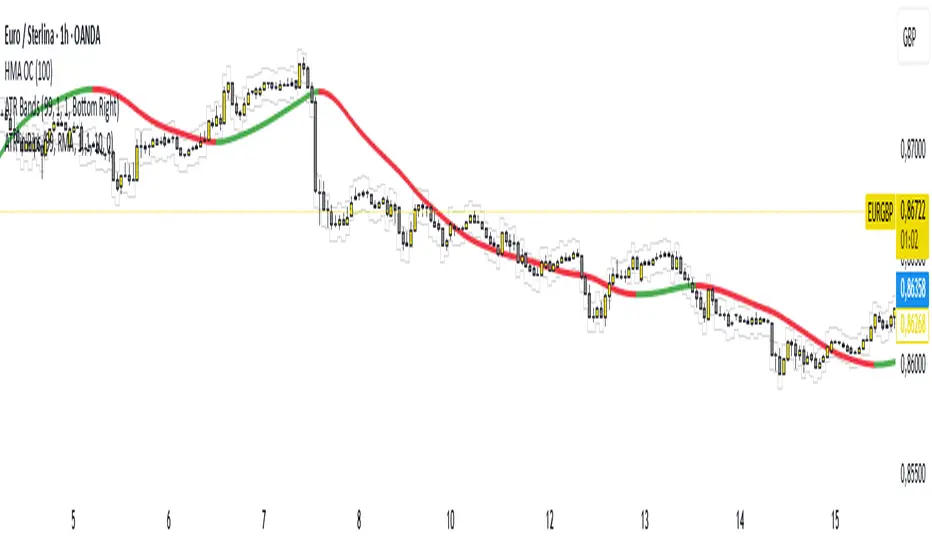
Volumetric Expansion/Contraction### Indicator Title: Volumetric Expansion/Contraction
### Summary
The Volumetric Expansion/Contraction (PCC) indicator is a comprehensive momentum oscillator designed to identify high-conviction price moves. Unlike traditional oscillators that only look at price, the PCC integrates four critical dimensions of market activity: **Price Change**, **Relative Volume (RVOL)**, **Cumulative Volume Delta (CVD)**, and **Average True Range (ATR)**.
Its primary purpose is to help traders distinguish between meaningful, volume-backed market expansions and noisy, unsustainable price action. It gives more weight to moves that occur in a controlled, low-volatility environment, highlighting potential starts of new trends or significant shifts in market sentiment.
### Key Concepts & Purpose
The indicator's unique formula synthesizes the following concepts:
1. **Price Change:** Measures the magnitude and direction of the primary move.
2. **Relative Volume (RVOL):** Confirms that the move is backed by significant volume compared to its recent average, indicating institutional participation.
3. **Cumulative Volume Delta (CVD):** Measures the underlying buying and selling pressure, confirming that the price move is aligned with the net flow of market orders.
4. **Inverse Volatility (ATR):** This is the indicator's unique twist. It normalizes the signal by the inverse of the Average True Range. This means the indicator's value is **amplified** when volatility (ATR) is low (signifying a controlled, confident expansion) and **dampened** when volatility is high (filtering out chaotic, less predictable moves).
The goal is to provide a single, easy-to-read oscillator that signals when price, volume, and order flow are all in alignment, especially during a breakout from a period of contraction.
### Features
* **Main Oscillator Line:** A single line plotted in a separate pane that represents the calculated strength of the volumetric expansion or contraction.
* **Zero Line:** A dotted reference line to easily distinguish between bullish (above zero) and bearish (below zero) regimes.
* **Visual Threshold Zones:** The background automatically changes color to highlight periods of significant strength:
* **Bright Green:** Indicates a "Strong Up Move" when the oscillator crosses above the user-defined upper threshold.
* **Bright Fuchsia:** Indicates a "Strong Down Move" when the oscillator crosses below the user-defined lower threshold.
### Configurable Settings & Filters
The indicator is fully customizable to allow for extensive testing and adaptation to different assets and timeframes.
#### Main Calculation Inputs
* **Price Change Lookback:** Sets the period for calculating the primary price change.
* **CVD Normalization Length:** The lookback period for normalizing the Cumulative Volume Delta.
* **RVOL Avg Volume Length:** The lookback for the simple moving average of volume, used to calculate RVOL.
* **RVOL Normalization Length:** The lookback period for normalizing the RVOL score.
* **ATR Length & Normalization Length:** Sets the periods for calculating the ATR and its longer-term average for normalization.
#### Weights
* Fine-tune the impact of each core component on the final calculation, allowing you to emphasize what matters most to your strategy (e.g., give more weight to CVD or RVOL).
#### External Market Filter (Powerful Feature)
* **Enable SPY/QQQ Filter for Up Moves?:** A checkbox to activate a powerful regime filter.
* **Symbol:** A dropdown to choose whether to filter signals based on the trend of **SPY** or **QQQ**.
* **SMA Period:** Sets the lookback period for the Simple Moving Average (default is 50).
* **How it works:** When enabled, this filter will **only allow "Strong Up Move" signals to appear if the chosen symbol (SPY or QQQ) is currently trading above its specified SMA**. This is an excellent tool for aligning your signals with the broader market trend and avoiding bullish entries in a bearish market.
#### Visuals
* **Upper/Lower Threshold:** Allows you to define what level the oscillator must cross to trigger the colored background zones, letting you customize the indicator's sensitivity.
***
**Disclaimer:** This tool is designed for market analysis and confluence. It is not a standalone trading system. Always use this indicator in conjunction with your own trading strategy, risk management, and other forms of analysis.

FVG Premium [no1x]█ OVERVIEW
This indicator provides a comprehensive toolkit for identifying, visualizing, and tracking Fair Value Gaps (FVGs) across three distinct timeframes (current chart, a user-defined Medium Timeframe - MTF, and a user-defined High Timeframe - HTF). It is designed to offer traders enhanced insight into FVG dynamics through detailed state monitoring (formation, partial fill, full mitigation, midline touch), extensive visual customization for FVG representation, and a rich alert system for timely notifications on FVG-related events.
█ CONCEPTS
This indicator is built upon the core concept of Fair Value Gaps (FVGs) and their significance in price action analysis, offering a multi-layered approach to their detection and interpretation across different timeframes.
Fair Value Gaps (FVGs)
A Fair Value Gap (FVG), also known as an imbalance, represents a range in price delivery where one side of the market (buying or selling) was more aggressive, leaving an inefficiency or an "imbalance" in the price action. This concept is prominently featured within Smart Money Concepts (SMC) and Inner Circle Trader (ICT) methodologies, where such gaps are often interpreted as footprints left by "smart money" due to rapid, forceful price movements. These methodologies suggest that price may later revisit these FVG zones to rebalance a prior inefficiency or to seek liquidity before continuing its path. These gaps are typically identified by a three-bar pattern:
Bullish FVG : This is a three-candle formation where the second candle shows a strong upward move. The FVG is the space created between the high of the first candle (bottom of FVG) and the low of the third candle (top of FVG). This indicates a strong upward impulsive move.
Bearish FVG : This is a three-candle formation where the second candle shows a strong downward move. The FVG is the space created between the low of the first candle (top of FVG) and the high of the third candle (bottom of FVG). This indicates a strong downward impulsive move.
FVGs are often watched by traders as potential areas where price might return to "rebalance" or find support/resistance.
Multi-Timeframe (MTF) Analysis
The indicator extends FVG detection beyond the current chart's timeframe (Low Timeframe - LTF) to two higher user-defined timeframes: Medium Timeframe (MTF) and High Timeframe (HTF). This allows traders to:
Identify FVGs that might be significant on a broader market structure.
Observe how FVGs from different timeframes align or interact.
Gain a more comprehensive perspective on potential support and resistance zones.
FVG State and Lifecycle Management
The indicator actively tracks the lifecycle of each detected FVG:
Formation : The initial identification of an FVG.
Partial Fill (Entry) : When price enters but does not completely pass through the FVG. The indicator updates the "current" top/bottom of the FVG to reflect the filled portion.
Midline (Equilibrium) Touch : When price touches the 50% level of the FVG.
Full Mitigation : When price completely trades through the FVG, effectively "filling" or "rebalancing" the gap. The indicator records the mitigation time.
This state tracking is crucial for understanding how price interacts with these zones.
FVG Classification (Large FVG)
FVGs can be optionally classified as "Large FVGs" (LV) if their size (top to bottom range) exceeds a user-defined multiple of the Average True Range (ATR) for that FVG's timeframe. This helps distinguish FVGs that are significantly larger relative to recent volatility.
Visual Customization and Information Delivery
A key concept is providing extensive control over how FVGs are displayed. This control is achieved through a centralized set of visual parameters within the indicator, allowing users to configure numerous aspects (colors, line styles, visibility of boxes, midlines, mitigation lines, labels, etc.) for each timeframe. Additionally, an on-chart information panel summarizes the nearest unmitigated bullish and bearish FVG levels for each active timeframe, providing a quick glance at key price points.
█ FEATURES
This indicator offers a rich set of features designed to provide a highly customizable and comprehensive Fair Value Gap (FVG) analysis experience. Users can tailor the FVG detection, visual representation, and alerting mechanisms across three distinct timeframes: the current chart (Low Timeframe - LTF), a user-defined Medium Timeframe (MTF), and a user-defined High Timeframe (HTF).
Multi-Timeframe FVG Detection and Display
The core strength of this indicator lies in its ability to identify and display FVGs from not only the current chart's timeframe (LTF) but also from two higher, user-selectable timeframes (MTF and HTF).
Timeframe Selection: Users can specify the exact MTF (e.g., "60", "240") and HTF (e.g., "D", "W") through dedicated inputs in the "MTF (Medium Timeframe)" and "HTF (High Timeframe)" settings groups. The visibility of FVGs from these higher timeframes can be toggled independently using the "Show MTF FVGs" and "Show HTF FVGs" checkboxes.
Consistent Detection Logic: The FVG detection logic, based on the classic three-bar imbalance pattern detailed in the 'Concepts' section, is applied consistently across all selected timeframes (LTF, MTF, HTF)
Timeframe-Specific Visuals: Each timeframe's FVGs (LTF, MTF, HTF) can be customized with unique colors for bullish/bearish states and their mitigated counterparts. This allows for easy visual differentiation of FVGs originating from different market perspectives.
Comprehensive FVG Visualization Options
The indicator provides extensive control over how FVGs are visually represented on the chart for each timeframe (LTF, MTF, HTF).
FVG Boxes:
Visibility: Main FVG boxes can be shown or hidden per timeframe using the "Show FVG Boxes" (for LTF), "Show Boxes" (for MTF/HTF) inputs.
Color Customization: Colors for bullish, bearish, active, and mitigated FVG boxes (including Large FVGs, if classified) are fully customizable for each timeframe.
Box Extension & Length: FVG boxes can either be extended to the right indefinitely ("Extend Boxes Right") or set to a fixed length in bars ("Short Box Length" or "Box Length" equivalent inputs).
Box Labels: Optional labels can display the FVG's timeframe and fill percentage on the box. These labels are configurable for all timeframes (LTF, MTF, and HTF). Please note: If FVGs are positioned very close to each other on the chart, their respective labels may overlap. This can potentially lead to visual clutter, and it is a known behavior in the current version of the indicator.
Box Borders: Visibility, width, style (solid, dashed, dotted), and color of FVG box borders are customizable per timeframe.
Midlines (Equilibrium/EQ):
Visibility: The 50% level (midline or EQ) of FVGs can be shown or hidden for each timeframe.
Style Customization: Width, style, and color of the midline are customizable per timeframe. The indicator tracks if this midline has been touched by price.
Mitigation Lines:
Visibility: Mitigation lines (representing the FVG's opening level that needs to be breached for full mitigation) can be shown or hidden for each timeframe. If shown, these lines are always extended to the right.
Style Customization: Width, style, and color of the mitigation line are customizable per timeframe.
Mitigation Line Labels: Optional price labels can be displayed on mitigation lines, with a customizable horizontal bar offset for positioning. For optimal label placement, the following horizontal bar offsets are recommended: 4 for LTF, 8 for MTF, and 12 for HTF.
Persistence After Mitigation: Users can choose to keep mitigation lines visible even after an FVG is fully mitigated, with a distinct color for such lines. Importantly, this option is only effective if the general setting 'Hide Fully Mitigated FVGs' is disabled, as otherwise, the entire FVG and its lines will be removed upon mitigation.
FVG State Management and Behavior
The indicator tracks and visually responds to changes in FVG states.
Hide Fully Mitigated FVGs: This option, typically found in the indicator's general settings, allows users to automatically remove all visual elements of an FVG from the chart once price has fully mitigated it. This helps maintain chart clarity by focusing on active FVGs.
Partial Fill Visualization: When price enters an FVG, the indicator offers a dynamic visual representation: the portion of the FVG that has been filled is shown as a "mitigated box" (typically with a distinct color), while the original FVG box shrinks to clearly highlight the remaining, unfilled portion. This two-part display provides an immediate visual cue about how much of the FVG's imbalance has been addressed and what potential remains within the gap.
Visual Filtering by ATR Proximity: To help users focus on the most relevant price action, FVGs can be dynamically hidden if they are located further from the current price than a user-defined multiple of the Average True Range (ATR). This behavior is controlled by the "Filter Band Width (ATR Multiple)" input; setting this to zero disables the filter entirely, ensuring all detected FVGs remain visible regardless of their proximity to price.
Alternative Usage Example: Mitigation Lines as Key Support/Resistance Levels
For traders preferring a minimalist chart focused on key Fair Value Gap (FVG) levels, the indicator's visualization settings can be customized to display only FVG mitigation lines. This approach leverages these lines as potential support and resistance zones, reflecting areas where price might revisit to address imbalances.
To configure this view:
Disable FVG Boxes: Turn off "Show FVG Boxes" (for LTF) or "Show Boxes" (for MTF/HTF) for the desired timeframes.
Hide Midlines: Disable the visibility of the 50% FVG Midlines (Equilibrium/EQ).
Ensure Mitigation Lines are Visible: Keep "Mitigation Lines" enabled.
Retain All Mitigation Lines:
Disable the "Hide Fully Mitigated FVGs" option in the general settings.
Enable the feature to "keep mitigation lines visible even after an FVG is fully mitigated". This ensures lines from all FVGs (active or fully mitigated) remain on the chart, which is only effective if "Hide Fully Mitigated FVGs" is disabled.
This setup offers:
A Decluttered Chart: Focuses solely on the FVG opening levels.
Precise S/R Zones: Treats mitigation lines as specific points for potential price reactions.
Historical Level Analysis: Includes lines from past, fully mitigated FVGs for a comprehensive view of significant price levels.
For enhanced usability with this focused view, consider these optional additions:
The on-chart Information Panel can be activated to display a quick summary of the nearest unmitigated FVG levels.
Mitigation Line Labels can also be activated for clear price level identification. A customizable horizontal bar offset is available for positioning these labels; for example, offsets of 4 for LTF, 8 for MTF, and 12 for HTF can be effective.
FVG Classification (Large FVG)
This feature allows for distinguishing FVGs based on their size relative to market volatility.
Enable Classification: Users can enable "Classify FVG (Large FVG)" to identify FVGs that are significantly larger than average.
ATR-Based Threshold: An FVG is classified as "Large" if its height (price range) is greater than or equal to the Average True Range (ATR) of its timeframe multiplied by a user-defined "Large FVG Threshold (ATR Multiple)". The ATR period for this calculation is also configurable.
Dedicated Colors: Large FVGs (both bullish/bearish and active/mitigated) can be assigned unique colors, making them easily distinguishable on the chart.
Panel Icon: Large FVGs are marked with a special icon in the Info Panel.
Information Panel
An on-chart panel provides a quick summary of the nearest unmitigated FVG levels.
Visibility and Position: The panel can be shown/hidden and positioned in any of the nine standard locations on the chart (e.g., Top Right, Middle Center).
Content: It displays the price levels of the nearest unmitigated bullish and bearish FVGs for LTF, MTF (if active), and HTF (if active). It also indicates if these nearest FVGs are Large FVGs (if classification is enabled) using a selectable icon.
Styling: Text size, border color, header background/text colors, default text color, and "N/A" cell background color are customizable.
Highlighting: Background and text colors for the cells displaying the overall nearest bullish and bearish FVG levels (across all active timeframes) can be customized to draw attention to the most proximate FVG.
Comprehensive Alert System
The indicator offers a granular alert system for various FVG-related events, configurable for each timeframe (LTF, MTF, HTF) independently. Users can enable alerts for:
New FVG Formation: Separate alerts for new bullish and new bearish FVG formations.
FVG Entry/Partial Fill: Separate alerts for price entering a bullish FVG or a bearish FVG.
FVG Full Mitigation: Separate alerts for full mitigation of bullish and bearish FVGs.
FVG Midline (EQ) Touch: Separate alerts for price touching the midline of a bullish or bearish FVG.
Alert messages are detailed, providing information such as the timeframe, FVG type (bull/bear, Large FVG), relevant price levels, and timestamps.
█ NOTES
This section provides additional information regarding the indicator's usage, performance considerations, and potential interactions with the TradingView platform. Understanding these points can help users optimize their experience and troubleshoot effectively.
Performance and Resource Management
Maximum FVGs to Track : The "Max FVGs to Track" input (defaulting to 25) limits the number of FVG objects processed for each category (e.g., LTF Bullish, MTF Bearish). Increasing this value significantly can impact performance due to more objects being iterated over and potentially drawn, especially when multiple timeframes are active.
Drawing Object Limits : To manage performance, this script sets its own internal limits on the number of drawing objects it displays. While it allows for up to approximately 500 lines (max_lines_count=500) and 500 labels (max_labels_count=500), the number of FVG boxes is deliberately restricted to a maximum of 150 (max_boxes_count=150). This specific limit for boxes is a key performance consideration: displaying too many boxes can significantly slow down the indicator, and a very high number is often not essential for analysis. Enabling all visual elements for many FVGs across all three timeframes can cause the indicator to reach these internal limits, especially the stricter box limit
Optimization Strategies : To help you manage performance, reduce visual clutter, and avoid exceeding drawing limits when using this indicator, I recommend the following strategies:
Maintain or Lower FVG Tracking Count: The "Max FVGs to Track" input defaults to 25. I find this value generally sufficient for effective analysis and balanced performance. You can keep this default or consider reducing it further if you experience performance issues or prefer a less dense FVG display.
Utilize Proximity Filtering: I suggest activating the "Filter Band Width (ATR Multiple)" option (found under "General Settings") to display only those FVGs closer to the current price. From my experience, a value of 5 for the ATR multiple often provides a good starting point for balanced performance, but you should feel free to adjust this based on market volatility and your specific trading needs.
Hide Fully Mitigated FVGs: I strongly recommend enabling the "Hide Fully Mitigated FVGs" option. This setting automatically removes all visual elements of an FVG from the chart once it has been fully mitigated by price. Doing so significantly reduces the number of active drawing objects, lessens computational load, and helps maintain chart clarity by focusing only on active, relevant FVGs.
Disable FVG Display for Unused Timeframes: If you are not actively monitoring certain higher timeframes (MTF or HTF) for FVG analysis, I advise disabling their display by unchecking "Show MTF FVGs" or "Show HTF FVGs" respectively. This can provide a significant performance boost.
Simplify Visual Elements: For active FVGs, consider hiding less critical visual elements if they are not essential for your specific analysis. This could include box labels, borders, or even entire FVG boxes if, for example, only the mitigation lines are of interest for a particular timeframe.
Settings Changes and Platform Limits : This indicator is comprehensive and involves numerous calculations and drawings. When multiple settings are changed rapidly in quick succession, it is possible, on occasion, for TradingView to issue a "Runtime error: modify_study_limit_exceeding" or similar. This can cause the indicator to temporarily stop updating or display errors.
Recommended Approach : When adjusting settings, it is advisable to wait a brief moment (a few seconds) after each significant change. This allows the indicator to reprocess and update on the chart before another change is made
Error Recovery : Should such a runtime error occur, making a minor, different adjustment in the settings (e.g., toggling a checkbox off and then on again) and waiting briefly will typically allow the indicator to recover and resume correct operation. This behavior is related to platform limitations when handling complex scripts with many inputs and drawing objects.
Multi-Timeframe (MTF/HTF) Data and Behavior
HTF FVG Confirmation is Essential: : For an FVG from a higher timeframe (MTF or HTF) to be identified and displayed on your current chart (LTF), the three-bar pattern forming the FVG on that higher timeframe must consist of fully closed bars. The indicator does not draw speculative FVGs based on incomplete/forming bars from higher timeframes.
Data Retrieval and LTF Processing: The indicator may use techniques like lookahead = barmerge.lookahead_on for timely data retrieval from higher timeframes. However, the actual detection of an FVG occurs after all its constituent bars on the HTF have closed.
Appearance Timing on LTF (1 LTF Candle Delay): As a natural consequence of this, an FVG that is confirmed on an HTF (i.e., its third bar closes) will typically become visible on your LTF chart one LTF bar after its confirmation on the HTF.
Example: Assume an FVG forms on a 30-minute chart at 15:30 (i.e., with the close of the 30-minute bar that covers the 15:00-15:30 period). If you are monitoring this FVG on a 15-minute chart, the indicator will detect this newly formed 30-minute FVG while processing the data for the 15-minute bar that starts at 15:30 and closes at 15:45. Therefore, the 30-minute FVG will become visible on your 15-minute chart at the earliest by 15:45 (i.e., with the close of that relevant 15-minute LTF candle). This means the HTF FVG is reflected on the LTF chart with a delay equivalent to one LTF candle.
FVG Detection and Display Logic
Fair Value Gaps (FVGs) on the current chart timeframe (LTF) are detected based on barstate.isconfirmed. This means the three-bar pattern must be complete with closed bars before an FVG is identified. This confirmation method prevents FVGs from being prematurely identified on the forming bar.
Alerts
Alert Setup : To receive alerts from this indicator, you must first ensure you have enabled the specific alert conditions you are interested in within the indicator's own settings (see 'Comprehensive Alert System' under the 'FEATURES' section). Once configured, open TradingView's 'Create Alert' dialog. In the 'Condition' tab, select this indicator's name, and crucially, choose the 'Any alert() function call' option from the dropdown list. This setup allows the indicator to trigger alerts based on the precise event conditions you have activated in its settings
Alert Frequency : Alerts are designed to trigger once per bar close (alert.freq_once_per_bar_close) for the specific event.
User Interface (UI) Tips
Settings Group Icons: In the indicator settings menu, timeframe-specific groups are marked with star icons for easier navigation: 🌟 for LTF (Current Chart Timeframe), 🌟🌟 for MTF (Medium Timeframe), and 🌟🌟🌟 for HTF (High Timeframe).
Dependent Inputs: Some input settings are dependent on others being enabled. These dependencies are visually indicated in the settings menu using symbols like "↳" (dependent setting on the next line), "⟷" (mutually exclusive inline options), or "➜" (directly dependent inline option).
Settings Layout Overview: The indicator settings are organized into logical groups for ease of use. Key global display controls – such as toggles for MTF FVGs, HTF FVGs (along with their respective timeframe selectors), and the Information Panel – are conveniently located at the very top within the '⚙️ General Settings' group. This placement allows for quick access to frequently adjusted settings. Other sections provide detailed customization options for each timeframe (LTF, MTF, HTF), specific FVG components, and alert configurations.
█ FOR Pine Script® CODERS
This section provides a high-level overview of the FVG Premium indicator's internal architecture, data flow, and the interaction between its various library components. It is intended for Pine Script™ programmers who wish to understand the indicator's design, potentially extend its functionality, or learn from its structure.
System Architecture and Modular Design
The indicator is architected moduarly, leveraging several custom libraries to separate concerns and enhance code organization and reusability. Each library has a distinct responsibility:
FvgTypes: Serves as the foundational data definition layer. It defines core User-Defined Types (UDTs) like fvgObject (for storing all attributes of an FVG) and drawSettings (for visual configurations), along with enumerations like tfType.
CommonUtils: Provides utility functions for common tasks like mapping user string inputs (e.g., "Dashed" for line style) to their corresponding Pine Script™ constants (e.g., line.style_dashed) and formatting timeframe strings for display.
FvgCalculations: Contains the core logic for FVG detection (both LTF and MTF/HTF via requestMultiTFBarData), FVG classification (Large FVGs based on ATR), and checking FVG interactions with price (mitigation, partial fill).
FvgObject: Implements an object-oriented approach by attaching methods to the fvgObject UDT. These methods manage the entire visual lifecycle of an FVG on the chart, including drawing, updating based on state changes (e.g., mitigation), and deleting drawing objects. It's responsible for applying the visual configurations defined in drawSettings.
FvgPanel: Manages the creation and dynamic updates of the on-chart information panel, which displays key FVG levels.
The main indicator script acts as the orchestrator, initializing these libraries, managing user inputs, processing data flow between libraries, and handling the main event loop (bar updates) for FVG state management and alerts.
Core Data Flow and FVG Lifecycle Management
The general data flow and FVG lifecycle can be summarized as follows:
Input Processing: User inputs from the "Settings" dialog are read by the main indicator script. Visual style inputs (colors, line styles, etc.) are consolidated into a types.drawSettings object (defined in FvgTypes). Other inputs (timeframes, filter settings, alert toggles) control the behavior of different modules. CommonUtils assists in mapping some string inputs to Pine constants.
FVG Detection:
For the current chart timeframe (LTF), FvgCalculations.detectFvg() identifies potential FVGs based on bar patterns.
For MTF/HTF, the main indicator script calls FvgCalculations.requestMultiTFBarData() to fetch necessary bar data from higher timeframes, then FvgCalculations.detectMultiTFFvg() identifies FVGs.
Newly detected FVGs are instantiated as types.fvgObject and stored in arrays within the main script. These objects also undergo classification (e.g., Large FVG) by FvgCalculations.
State Update & Interaction: On each bar, the main indicator script iterates through active FVG objects to manage their state based on price interaction:
Initially, the main script calls FvgCalculations.fvgInteractionCheck() to efficiently determine if the current bar's price might be interacting with a given FVG.
If a potential interaction is flagged, the main script then invokes methods directly on the fvgObject instance (e.g., updateMitigation(), updatePartialFill(), checkMidlineTouch(), which are part of FvgObject).
These fvgObject methods are responsible for the detailed condition checking and the actual modification of the FVG's state. For instance, the updateMitigation() and updatePartialFill() methods internally utilize specific helper functions from FvgCalculations (like checkMitigation() and checkPartialMitigation()) to confirm the precise nature of the interaction before updating the fvgObject’s state fields (such as isMitigated, currentTop, currentBottom, or isMidlineTouched).
Visual Rendering:
The FvgObject.updateDrawings() method is called for each fvgObject. This method is central to drawing management; it creates, updates, or deletes chart drawings (boxes, lines, labels) based on the FVG's current state, its prev_* (previous bar state) fields for optimization, and the visual settings passed via the drawSettings object.
Information Panel Update: The main indicator script determines the nearest FVG levels, populates a panelData object (defined in FvgPanelLib), and calls FvgPanel.updatePanel() to refresh the on-chart display.
Alert Generation: Based on the updated FVG states and user-enabled alert settings, the main indicator script constructs and triggers alerts using Pine Script's alert() function."
Key Design Considerations
UDT-Centric Design: The fvgObject UDT is pivotal, acting as a stateful container for all information related to a single FVG. Most operations revolve around creating, updating, or querying these objects.
State Management: To optimize drawing updates and manage FVG lifecycles, fvgObject instances store their previous bar's state (e.g., prevIsVisible, prevCurrentTop). The FvgObject.updateDrawings() method uses this to determine if a redraw is necessary, minimizing redundant drawing calls.
Settings Object: A drawSettings object is populated once (or when inputs change) and passed to drawing functions. This avoids repeatedly reading numerous input() values on every bar or within loops, improving performance.
Dynamic Arrays for FVG Storage: Arrays are used to store collections of fvgObject instances, allowing for dynamic management (adding new FVGs, iterating for updates).

Test OHLCV LibraryThis indicator, "Test OHLCV Library," serves as a practical example of how to use the OHLCVData library to fetch historical candle data from a specific timeframe (like 4H) in a way that is largely impervious to the chart's currently selected time frame.
Here's a breakdown of its purpose and how it addresses request.security limitations:
Indicator Purpose:
The main goal of this indicator is to demonstrate and verify that the OHLCVData library can reliably provide confirmed historical OHLCV data for a user-specified timeframe (e.g., 4H), and that a collection of these data points (the last 10 completed candles) remains consistent even when the user switches the chart's time frame (e.g., from 5-second to Daily).
It does this by:
Importing the OHLCVData library.
Using the library's getTimeframeData function on every bar of the chart.
Checking the isTargetBarClosed flag returned by the library to identify the exact moment a candle in the target timeframe (e.g., 4H) has closed.
When isTargetBarClosed is true, it captures the confirmed OHLCV data provided by the library for that moment and stores it in a persistent var array.
It maintains a list of the last 10 captured historical 4H candle opens in this array.
It displays these last 10 confirmed opens in a table.
It uses the isAdjustedToChartTF flag from the library to show a warning if the chart's time frame is higher than the target timeframe, indicating that the data fetched by request.security is being aligned to that higher resolution.
Circumventing request.security Limitations:
The primary limitation of request.security that this setup addresses is the challenge of getting a consistent, non-repainting collection of historical data points from a different timeframe when the chart's time frame is changed.
The Problem: Standard request.security calls, while capable of fetching data from other timeframes, align that data to the bars of the current chart. When you switch the chart's time frame, the set of chart bars changes, and the way the requested data aligns to these new bars changes. If you simply collected data on every chart bar where request.security returned a non-na value, the resulting collection would differ depending on the chart's resolution. Furthermore, using request.security without lookahead=barmerge.lookahead_off or an offset ( ) can lead to repainting on historical bars, where values change as the script recalculates.
How the Library/Indicator Setup Helps:
Confirmed Data: The OHLCVData library uses lookahead=barmerge.lookahead_off and, more importantly, provides the isTargetBarClosed flag. This flag is calculated using a reliable method (checking for a change in the target timeframe's time series) that accurately identifies the precise chart bar corresponding to the completion of a candle in the target timeframe (e.g., a 4H candle), regardless of the chart's time frame.
Precise Capture: The indicator only captures and stores the OHLCV data into its var array when this isTargetBarClosed flag is true. This means it's capturing the confirmed, finalized data for the target timeframe candle at the exact moment it closes.
Persistent Storage: The var array in the indicator persists its contents across the bars of the chart's history. As the script runs through the historical bars, it selectively adds confirmed 4H candle data points to this array only when the trigger is met.
Impervious Collection: Because the array is populated based on the completion of the target timeframe candles (detected reliably by the library) rather than simply collecting data on every chart bar, the final contents of the array (the list of the last 10 confirmed 4H opens) will be the same regardless of the chart's time frame. The table then displays this static collection.
In essence, this setup doesn't change how request.security fundamentally works or aligns data to the chart's bars. Instead, it uses the capabilities of request.security (fetching data from another timeframe) and Pine Script's execution model (bar-by-bar processing, var persistence) in a specific way, guided by the library's logic, to build a historical collection of data points that represent the target timeframe's candles and are independent of the chart's display resolution.

BySq - Market PsychologyThe script I provided is a Market Psychology Index indicator for TradingView, which focuses on three key psychological market phases:
FOMO (Fear of Missing Out)
Panic Selling
Reversal
This indicator uses volume, price changes, and specific time periods to gauge market sentiment. Let me break it down:
1. Input Parameters:
FOMO Period: Defines how many bars (candles) the FOMO index will consider for its calculation.
Panic Period: Defines the period to evaluate Panic Selling.
Reversal Period: Defines the period to evaluate potential price reversals.
You can adjust these periods based on your analysis preferences. The default for each period is 14.
2. FOMO Index:
The FOMO Index aims to capture the "fear of missing out" behavior in the market.
It uses volume and price change:
Volume is compared to the Simple Moving Average (SMA) of volume over the specified period.
Price change is calculated as the percentage change in price compared to the previous bar.
If both volume and price change indicate strong upward movement, the FOMO index spikes.
3. Panic Selling Index:
The Panic Selling Index captures when traders are selling out of fear, often in a rapid or irrational way.
Similar to the FOMO Index, it considers volume and price change:
It uses volume and compares it to the SMA of volume for the panic period.
Price change is negative, meaning it considers only price drops.
When there is high volume coupled with significant price drops, it signals panic selling.
4. Reversal Index:
The Reversal Index aims to detect potential trend reversals in the market.
This index also considers volume and price change:
It focuses on upward price movement and compares volume to its SMA.
If there’s strong upward price movement along with increasing volume, it signals the possibility of a price reversal.
5. Graphical Output:
Histograms are drawn on the chart for each of the three indices:
FOMO is shown in green (indicating the presence of FOMO) and red (when the index is low).
Panic Selling is shown in orange.
Reversal is shown in purple.
The Zero Line (horizontal dotted line) helps identify when any of the indices is positive or negative.
6. Labels:
Labels for each index are shown on the chart at the relevant bar when the index spikes.
FOMO is labeled "FOMO" in green when it spikes.
Panic Selling is labeled "Panic Selling" in orange when it spikes.
Reversal is labeled "Reversal" in purple when it spikes.
Additionally, period labels show above the chart, indicating the specific periods (FOMO, Panic, and Reversal periods) currently being applied. This provides clarity on what time frame each index is analyzing.
7. How to Use:
FOMO: High values may indicate that traders are buying out of fear of missing out on a rally, suggesting a potentially overheated market.
Panic Selling: High values could suggest irrational selling behavior or capitulation, potentially marking the bottom of a downtrend.
Reversal: High values signal the potential for a market reversal, where the price could change direction due to increased volume and upward movement.
8. Visual Appearance:
The indicator’s histograms change colors based on the level of market sentiment detected. The color-coded approach provides an easy-to-read visual representation of different psychological phases in the market.
The horizontal zero line allows easy differentiation between positive and negative values.
Summary:
This script combines the psychology of the market (FOMO, Panic Selling, and Reversal) into a set of indicators that help traders identify potential turning points or emotional states in the market. By focusing on volume and price change, the script attempts to give a clear picture of market sentiment and possible future movements.

Follow Line Strategy Version 2.5 (React HTF)Follow Line Strategy v2.5 (React HTF) - TradingView Script Usage
This strategy utilizes a "Follow Line" concept based on Bollinger Bands and ATR to identify potential trading opportunities. It includes advanced features like optional working hours filtering, higher timeframe (HTF) trend confirmation, and improved trend-following entry/exit logic. Version 2.5 introduces reactivity to HTF trend changes for more adaptive trading.
Key Features:
Follow Line: The core of the strategy. It dynamically adjusts based on price breakouts beyond Bollinger Bands, using either the low/high or ATR-adjusted levels.
Bollinger Bands: Uses a standard Bollinger Bands setup to identify overbought/oversold conditions.
ATR Filter: Optionally uses the Average True Range (ATR) to adjust the Follow Line offset, providing a more dynamic and volatility-adjusted entry point.
Optional Trading Session Filter: Allows you to restrict trading to specific hours of the day.
Higher Timeframe (HTF) Confirmation: A significant feature that allows you to confirm trade signals with the trend on a higher timeframe. This can help to filter out false signals and improve the overall win rate.
HTF Selection Method: Choose between Auto and Manual HTF selection:
Auto: The script automatically determines the appropriate HTF based on the current chart timeframe (e.g., 1min -> 15min, 5min -> 4h, 1h -> 1D, Daily -> Monthly).
Manual: Allows you to select a specific HTF using the Manual Higher Timeframe input.
Trend-Following Entries/Exits: The strategy aims to enter trades in the direction of the established trend, using the Follow Line to define the trend.
Reactive HTF Trend Changes: v2.5 exits positions not only based on the trade timeframe (TTF) trend changing, but also when the higher timeframe trend reverses against the position. This makes the strategy more responsive to larger market movements.
Alerts: Provides buy and sell alerts for convenient trading signal notifications.
Visualizations: Plots the Follow Line for both the trade timeframe and the higher timeframe (optional), making it easy to understand the strategy's logic.
How to Use:
Add to Chart: Add the "Follow Line Strategy Version 2.5 (React HTF)" script to your TradingView chart.
Configure Settings: Customize the strategy's settings to match your trading style and preferences. Here's a breakdown of the key settings:
Indicator Settings:
ATR Period: The period used to calculate the ATR. A smaller period is more sensitive to recent price changes.
Bollinger Bands Period: The period used for the Bollinger Bands calculation. A longer period results in smoother bands.
Bollinger Bands Deviation: The number of standard deviations from the moving average that the Bollinger Bands are plotted. Higher deviations create wider bands.
Use ATR for Follow Line Offset?: Enable to use ATR to calculate the Follow Line offset. Disable to use the simple high/low.
Show Trade Signals on Chart?: Enable to show BUY/SELL labels on the chart.
Time Filter:
Use Trading Session Filter?: Enable to restrict trading to specific hours of the day.
Trading Session: The trading session to use (e.g., 0930-1600 for regular US stock market hours). Use 0000-2400 for all hours.
Higher Timeframe Confirmation:
Enable HTF Confirmation?: Enable to use the HTF trend to filter trade signals. If enabled, only trades in the direction of the HTF trend will be taken.
HTF Selection Method: Choose between "Auto" and "Manual" HTF selection.
Manual Higher Timeframe: If "Manual" is selected, choose the specific HTF (e.g., 240 for 4 hours, D for daily).
Show HTF Follow Line?: Enable to plot the HTF Follow Line on the chart.
Understanding the Signals:
Buy Signal: The price breaks above the upper Bollinger Band, and the HTF (if enabled) confirms the uptrend.
Sell Signal: The price breaks below the lower Bollinger Band, and the HTF (if enabled) confirms the downtrend.
Exit Long: The trade timeframe trend changes to downtrend or the higher timeframe trend changes to downtrend.
Exit Short: The trade timeframe trend changes to uptrend or the higher timeframe trend changes to uptrend.
Alerts:
The script includes alert conditions for buy and sell signals. To set up alerts, click the "Alerts" button in TradingView and select the desired alert condition from the script. The alert message provides the ticker and interval.
Backtesting and Optimization:
Use TradingView's Strategy Tester to backtest the strategy on different assets and timeframes.
Experiment with different settings to optimize the strategy for your specific trading style and risk tolerance. Pay close attention to the ATR Period, Bollinger Bands settings, and the HTF confirmation options.
Tips and Considerations:
HTF Confirmation: The HTF confirmation can significantly improve the strategy's performance by filtering out false signals. However, it can also reduce the number of trades.
Risk Management: Always use proper risk management techniques, such as stop-loss orders and position sizing, when trading any strategy.
Market Conditions: The strategy may perform differently in different market conditions. It's important to backtest and optimize the strategy for the specific markets you are trading.
Customization: Feel free to modify the script to suit your specific needs. For example, you could add additional filters or entry/exit conditions.
Pyramiding: The pyramiding = 0 setting prevents multiple entries in the same direction, ensuring the strategy doesn't compound losses. You can adjust this value if you prefer to pyramid into winning positions, but be cautious.
Lookahead: The lookahead = barmerge.lookahead_off setting ensures that the HTF data is calculated based on the current bar's closed data, preventing potential future peeking bias.
Trend Determination: The logic for determining the HTF trend and reacting to changes is critical. Carefully review the f_calculateHTFData function and the conditions for exiting positions to ensure you understand how the strategy responds to different market scenarios.
Disclaimer:
This script is for informational and educational purposes only. It is not financial advice, and you should not trade based solely on the signals generated by this script. Always do your own research and consult with a qualified financial advisor before making any trading decisions. The author is not responsible for any losses incurred as a result of using this script.
