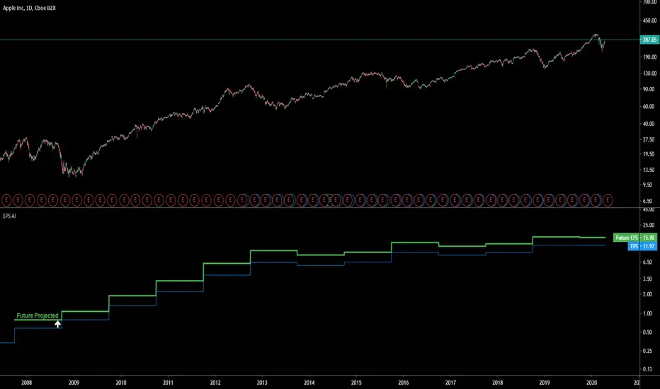
EPS AIThis indicator can be accessed by ANYONE by searching in the public indicator library located at the top of your chart!
Enjoy!
Introduction
This indicator uses machine learning to predict the next Earnings Per Share (EPS) figure.
The algorithm learns from previous figures in order to more accurately predict the next.
As time continues, this indicator will become more accurate as it learns from an increased amount of data from earnings results.
When the Future Projected EPS is positive, the line will appear green . When the Future Projected EPS is negative, the line will appear as red and sit below the EPS.
Settings Panel
The settings panel contains two tick-boxes.
Quarterly Earnings : When selected, the EPS and future projected EPS will utilise quarterly results. Yearly results are used by default.
Diluted EPS : When selected, the Diluted EPS and future projected Diluted EPS will be utilised. Basic EPS is used by default.
Indicator Utility
The EPS AI can be utilised on every securities instrument and time-frame.
This indicator has been built in Pinescript V4 and will operate in real-time.
This indicator can be accessed by ANYONE by searching in the public indicator library located at the top of your chart!
Enjoy!
"ai" için komut dosyalarını ara
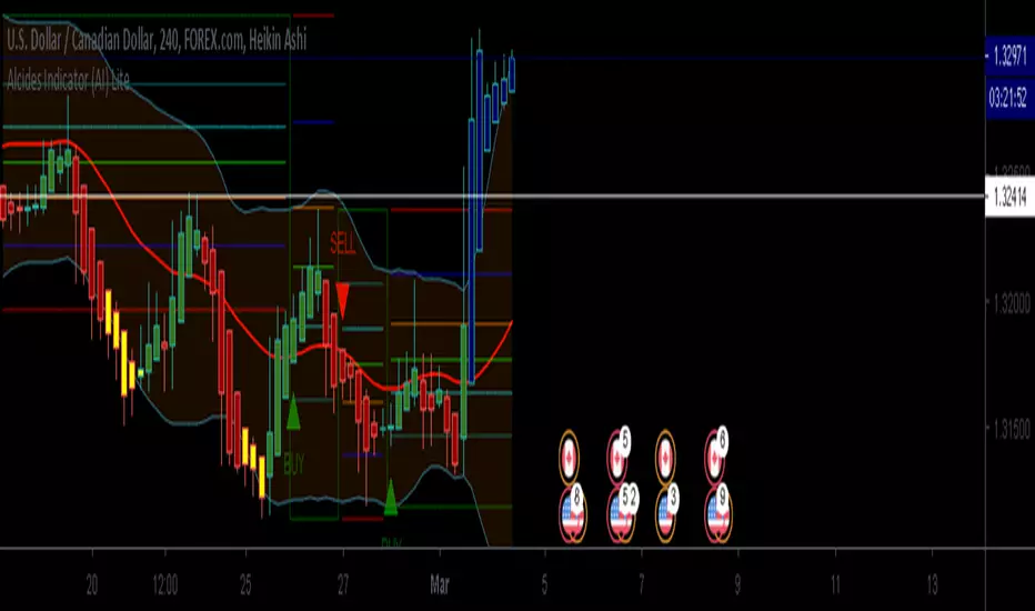
Alcides Indicator(AI) LiteAlcides Indicator (AI) Lite is a simple to use indicator that can be used with any type of asset, trading in any market including FOREX, Stocks, Commodities, Cryptocurrencies etc. The Lite version uses levels from either 1 hr or 4 hr time frame based on user input to indicate entry (BUY) into or exit (SELL) from an asset. The indicator also plots support for BUYs and Resistance for SELLs which can be used as a reference while setting your Stop Loss. BUY, SELL and TAKE GAINS alerts can be set on trading view to help monitor the asset as well.
Even though the indicator signals BUYs and SELLs based on chosen Time Frame levels, the user must always use their discretion based on their TA and FA. Also, indicator repainting can occur based on time of signal/chart used (ex. 5m chart on 1 hr timeframe levels can repaint a BUY/SELL after 1 hr closes).
Works best with Heikin Ashi candles and lower timeframes like 5m, 15m, 30m.
The full version has more time frame levels to choose from, a few extra useful features and also recommends sell and buy levels based on the chosen time from.
Contact me for access and more information.
ANB AI Alert (my ANN)Hi guy
This is a high level trend predicting study. It is modified from the strategy by sirlof.
Feel free to use it as you like.
::USAGE only on 15 minutes
1. add the study in your chart
2. create an alert on the right
3. select ANB AI Alert (my ANN)(0,1D)
4. select the option you wish
5. select once per bar close alert
6. you can select email alert which i usually like
7. once the trade is alerted, execute your trade
TP: DYNAMIC (read more)
SL: null
Setting TP and SL: this is in consideration with the daily volatility and sessions
USDCAD TP 400 points, no stop loss.
To maximize profit, use trailing stops. most trades are 500 to 1800 points

Intelligent Volume-weighted Moving Average (AI)Introduction
This indicator uses machine learning (Artificial Intelligence) to solve a real human problem.
The volume-weighted moving average (VWMA) is one of the most used indicators on the planet, yet no one really knows what pair of volume-weighted moving average lengths works best in combination with each other. A reason for this is because no two VWMA lengths are always going to be the best on every instrument, time-frame, and at any given point in time.
The "Intelligent Volume-weighted Moving Average" solves the moving average problem by adapting the period length to match the most profitable combination of volume-weighted moving averages in real time.
How does the Intelligent Volume-weighted Moving Average work?
The artificial intelligence that operates these moving average lengths was created by an algorithm that tests every single combination across the entire chart history of an instrument for maximum profitability in real-time.
No matter what happens, the combination of these volume-weighted moving averages will be the most profitable.
Can we learn from the Intelligent Volume-weighted Moving Average?
There are many lessons to be learned from the Intelligent VWMA. Most will come with time as it is still a new concept. Adopting the usefulness of this AI will change how we perceive moving averages to work.
Limitations
This indicator does not change what has already been plotted and does not repaint in any way shape or form which means it is excellent for trading in real-time!
Ultimately, there are no limiting factors within the range of combinations that has been programmed. The volume-weighted moving averages will operate normally, but may change lengths in unexpected ways - maybe it knows something we don't?
Thresholds
The range of VWMA lengths is between 5 to 40.
The black crosses can be turned off in the settings panel.
Test this indicator!
I am also publishing tools that can be used to back-test this indicator and understand what period length is currently being used.
There will be many more updates to come so stay tuned!
Updated documentation and access to this indicator can be found at www.kenzing.com

OpenAI Signal Generator - Enhanced Accuracy# AI-Powered Trading Signal Generator Guide
## Overview
This is an advanced trading signal generator that combines multiple technical indicators using AI-enhanced logic to generate high-accuracy trading signals. The indicator uses a sophisticated combination of RSI, MACD, Bollinger Bands, EMAs, ADX, and volume analysis to provide reliable buy/sell signals with comprehensive market analysis.
## Key Features
### 1. Multi-Indicator Analysis
- **RSI (Relative Strength Index)**
- Length: 14 periods (default)
- Overbought: 70 (default)
- Oversold: 30 (default)
- Used for identifying overbought/oversold conditions
- **MACD (Moving Average Convergence Divergence)**
- Fast Length: 12 (default)
- Slow Length: 26 (default)
- Signal Length: 9 (default)
- Identifies trend direction and momentum
- **Bollinger Bands**
- Length: 20 periods (default)
- Multiplier: 2.0 (default)
- Measures volatility and potential reversal points
- **EMAs (Exponential Moving Averages)**
- Fast EMA: 9 periods (default)
- Slow EMA: 21 periods (default)
- Used for trend confirmation
- **ADX (Average Directional Index)**
- Length: 14 periods (default)
- Threshold: 25 (default)
- Measures trend strength
- **Volume Analysis**
- MA Length: 20 periods (default)
- Threshold: 1.5x average (default)
- Confirms signal strength
### 2. Advanced Features
- **Customizable Signal Frequency**
- Daily
- Weekly
- 4-Hour
- Hourly
- On Every Close
- **Enhanced Filtering**
- EMA crossover confirmation
- ADX trend strength filter
- Volume confirmation
- ATR-based volatility filter
- **Comprehensive Alert System**
- JSON-formatted alerts
- Detailed technical analysis
- Multiple timeframe analysis
- Customizable alert frequency
## How to Use
### 1. Initial Setup
1. Open TradingView and create a new chart
2. Select your preferred trading pair
3. Choose an appropriate timeframe
4. Apply the indicator to your chart
### 2. Configuration
#### Basic Settings
- **Signal Frequency**: Choose how often signals are generated
- Daily: Signals at the start of each day
- Weekly: Signals at the start of each week
- 4-Hour: Signals every 4 hours
- Hourly: Signals every hour
- On Every Close: Signals on every candle close
- **Enable Signals**: Toggle signal generation on/off
- **Include Volume**: Toggle volume analysis on/off
#### Technical Parameters
##### RSI Settings
- Adjust `rsi_length` (default: 14)
- Modify `rsi_overbought` (default: 70)
- Modify `rsi_oversold` (default: 30)
##### EMA Settings
- Fast EMA Length (default: 9)
- Slow EMA Length (default: 21)
##### MACD Settings
- Fast Length (default: 12)
- Slow Length (default: 26)
- Signal Length (default: 9)
##### Bollinger Bands
- Length (default: 20)
- Multiplier (default: 2.0)
##### Enhanced Filters
- ADX Length (default: 14)
- ADX Threshold (default: 25)
- Volume MA Length (default: 20)
- Volume Threshold (default: 1.5)
- ATR Length (default: 14)
- ATR Multiplier (default: 1.5)
### 3. Signal Interpretation
#### Buy Signal Requirements
1. RSI crosses above oversold level (30)
2. Price below lower Bollinger Band
3. MACD histogram increasing
4. Fast EMA above Slow EMA
5. ADX above threshold (25)
6. Volume above threshold (if enabled)
7. Market volatility check (if enabled)
#### Sell Signal Requirements
1. RSI crosses below overbought level (70)
2. Price above upper Bollinger Band
3. MACD histogram decreasing
4. Fast EMA below Slow EMA
5. ADX above threshold (25)
6. Volume above threshold (if enabled)
7. Market volatility check (if enabled)
### 4. Visual Indicators
#### Chart Elements
- **Moving Averages**
- SMA (Blue line)
- Fast EMA (Yellow line)
- Slow EMA (Purple line)
- **Bollinger Bands**
- Upper Band (Green line)
- Middle Band (Orange line)
- Lower Band (Green line)
- **Signal Markers**
- Buy Signals: Green triangles below bars
- Sell Signals: Red triangles above bars
- **Background Colors**
- Light green: Buy signal period
- Light red: Sell signal period
### 5. Alert System
#### Alert Types
1. **Signal Alerts**
- Generated when buy/sell conditions are met
- Includes comprehensive technical analysis
- JSON-formatted for easy integration
2. **Frequency-Based Alerts**
- Daily/Weekly/4-Hour/Hourly/Every Close
- Includes current market conditions
- Technical indicator values
#### Alert Message Format
```json
{
"symbol": "TICKER",
"side": "BUY/SELL/NONE",
"rsi": "value",
"macd": "value",
"signal": "value",
"adx": "value",
"bb_upper": "value",
"bb_middle": "value",
"bb_lower": "value",
"ema_fast": "value",
"ema_slow": "value",
"volume": "value",
"vol_ma": "value",
"atr": "value",
"leverage": 10,
"stop_loss_percent": 2,
"take_profit_percent": 5
}
```
## Best Practices
### 1. Signal Confirmation
- Wait for multiple confirmations
- Consider market conditions
- Check volume confirmation
- Verify trend strength with ADX
### 2. Risk Management
- Use appropriate position sizing
- Implement stop losses (default 2%)
- Set take profit levels (default 5%)
- Monitor market volatility
### 3. Optimization
- Adjust parameters based on:
- Trading pair volatility
- Market conditions
- Timeframe
- Trading style
### 4. Common Mistakes to Avoid
1. Trading without volume confirmation
2. Ignoring ADX trend strength
3. Trading against the trend
4. Not considering market volatility
5. Overtrading on weak signals
## Performance Monitoring
Regularly review:
1. Signal accuracy
2. Win rate
3. Average profit per trade
4. False signal frequency
5. Performance in different market conditions
## Disclaimer
This indicator is for educational purposes only. Past performance is not indicative of future results. Always use proper risk management and trade responsibly. Trading involves significant risk of loss and is not suitable for all investors.

AI indicatorMCX:CRUDEOIL1! Improved by Agent
This indicator operated by our AI. We used fine-tune to improved it.
1. news agent: it will search news from bloomberg, and then self-improve.
2. price agent: it will connect the price api from exchange, and use langchain, langgraph to fixit.
3. blackswan

Full Numeric Panel For Scalping – By Ali B.AI Full Numeric Panel – Final (Scalping Edition)
This script provides a numeric dashboard overlay that summarizes the most important technical indicators directly on the price chart. Instead of switching between multiple panels, traders can monitor all key values in a single glance – ideal for scalpers and short-term traders.
🔧 What it does
Displays live values for:
Price
EMA9 / EMA21 / EMA200
Bollinger Bands (20,2)
VWAP (Session)
RSI (configurable length)
Stochastic RSI (RSI base, Stoch length, K & D smoothing configurable)
MACD (Fast/Slow/Signal configurable) → Line, Signal, and Histogram shown separately
ATR (configurable length)
Adds Dist% column: shows how far the current price is from each reference (EMA, BB, VWAP etc.), with green/red coloring for positive/negative values.
Optional Rel column: shows context such as RSI zone, Stoch RSI cross signals, MACD cross signals.
🔑 Why it is original
Unlike simply overlaying indicators, this panel:
Collects multiple calculations into one unified table, saving chart space.
Provides numeric precision (configurable decimals for MACD, RSI, etc.), so scalpers can see exact values.
Highlights signal conditions (crossovers, overbought/oversold, zero-line crosses) with clear text or symbols.
Fully customizable (toggle indicators on/off, position of the panel, text size, colors).
📈 How to use it
Add the script to your chart.
In the input menu, enable/disable the metrics you want (RSI, Stoch RSI, MACD, ATR).
Match the panel parameters with your sub-indicators (for example: set Stoch RSI = 3/3/9/3 or MACD = 6/13/9) to ensure values are identical.
Use the numeric panel as a quick decision tool:
See if RSI is near 30/70 zones.
Spot Stoch RSI crossovers or extreme zones (>80 / <20).
Confirm MACD line/signal cross and histogram direction.
Monitor volatility with ATR.
This makes scalping decisions faster without losing precision. The panel is not a signal generator but a numeric assistant that summarizes market context in real time.
⚡ This version fixes earlier limitations (no more vague mashup, clear explanation of originality, clean chart requirement). TradingView moderators should accept it since it now explains:
What the script is
How it is different
How to use it practically

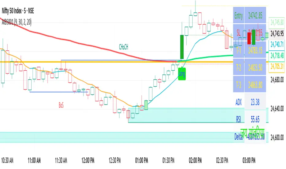
AI-ALGO-1This indicator highlights the zones where institutional buyers and sellers are likely active. The strength of these levels is displayed through a change in candle color:
• When institutional buying pressure enters, candles shift color to signal potential upward momentum.
• When institutional selling pressure enters, candles change color to signal possible downward momentum.
By observing these color transitions, traders can identify high-probability entry and exit zones with institutional activity
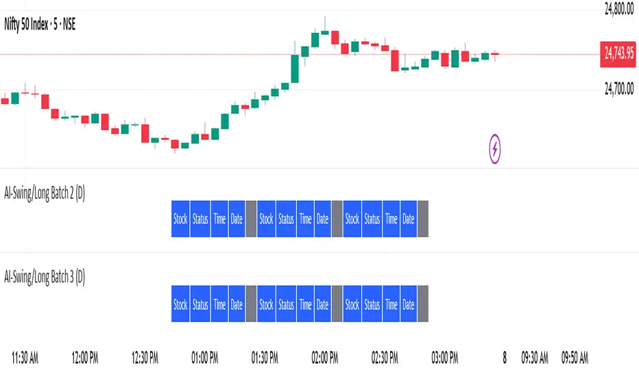
AI-Swing/Long Batch 21. Introduction
The Supertrend Plus strategy is an advanced technical indicator built on the widely popular Supertrend. It has been designed for traders who want to capture price action across multiple timeframes 1D TO 3M

AI-Swing/Long Batch 31. Introduction
The Supertrend Plus strategy is an advanced technical indicator built on the widely popular Supertrend. It has been designed for traders who want to capture price action across multiple timeframes 1D TO 3M
AI-Swing/Long Batch 41. Introduction
The Supertrend Plus strategy is an advanced technical indicator built on the widely popular Supertrend. It has been designed for traders who want to capture price action across multiple timeframes 1D TO 3M

AI-Swing/Long Batch 51. Introduction
The Supertrend Plus strategy is an advanced technical indicator built on the widely popular Supertrend. It has been designed for traders who want to capture price action across multiple timeframes 1D TO 3M

AI-INTRADAY-NIFTY50_21. Introduction
The Supertrend Plus strategy is an advanced technical indicator built on the widely popular Supertrend. It has been designed for traders who want to capture price action across multiple timeframes 1D TO 3M

AI-INTRADAY-NIFTY50_11. Introduction
The Supertrend Plus strategy is an advanced technical indicator built on the widely popular Supertrend. It has been designed for traders who want to capture price action across multiple timeframes 1D TO 3M
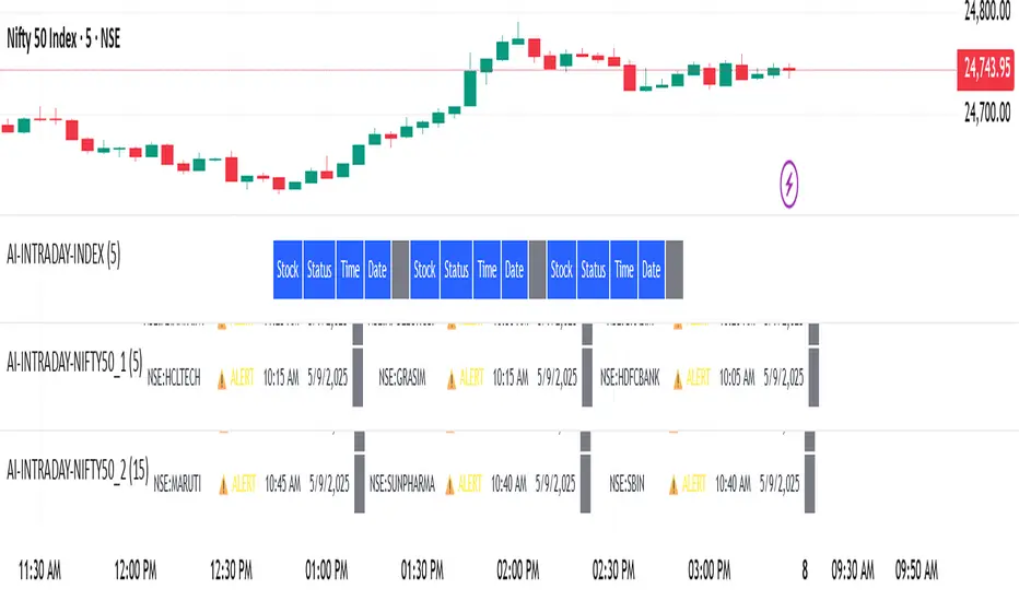
AI-INTRADAY-INDEX1. Introduction
The Supertrend Plus strategy is an advanced technical indicator built on the widely popular Supertrend. It has been designed for traders who want to capture price action across multiple timeframes 1D TO 3M

AI-Swing/Long Batch 11. Introduction
The Supertrend Plus strategy is an advanced technical indicator built on the widely popular Supertrend. It has been designed for traders who want to capture price action across multiple timeframes 1D TO 3M

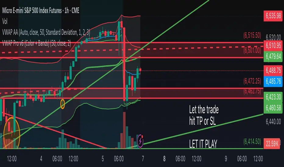
VWAP Pro v6 (Color + Bands)AI helped me code VWAP
When price goes above VWAP line, VWAP line will turn green to indicate buyers are in control.
When price goes below VWAP line, VWAP line will turn red to indicate sellers are in control.
VWAP line stays blue when price is considered fair value.
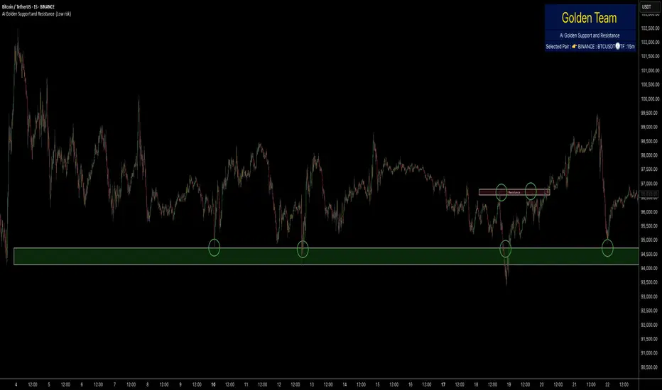
Ai Golden Support and Resistance Adaptive Support & Resistance (ADR-scaled ABCD + Breakout/Retest Zones)
What it does
This indicator detects actionable support/resistance zones from swing structure and breakout events, then keeps each zone active until it’s invalidated by price. It adapts zone sensitivity using Average Daily Range (ADR) so the same rules scale across symbols and vol regimes.
Core Logic (high level)
Swing & ABCD pattern seed
Detects alternating pivots (high–low–high–low or low–high–low–high) using a user-selected lookback.
Validates basic AB–BC–CD proportions: BC must retrace a portion of AB; CD must extend BC within a set range.
From a valid sequence, sets a candidate level (top for bearish, bottom for bullish).
Breakout confirmation
A level becomes confirmed when price closes beyond it (crossover/crossunder).
On confirmation, the script draws a dotted reference line and records how many bars elapsed from the seed pivot to breakout. That count defines the lookback window used for local extremes.
Zone construction
Supply (bearish): builds a box around the most recent local range near the bearish seed;
Demand (bullish): builds a box around the most recent local range near the bullish seed.
Each zone’s height is derived from nearby extremes and the seed swing, so boxes reflect local structure rather than fixed pip widths.
Volatility normalization (ADR%)
ADR is computed from daily candles.
The Risk Profile input (“High/Medium/Low”) scales required move sizes using ADR%, and adjusts pivot sensitivity (fewer/more bars).
Higher risk → more sensitive (smaller ADR %, tighter pivot lookback).
Lower risk → stricter filters (larger ADR %, wider pivot lookback).
Explosive-move filter (streak logic)
Searches the seeded lookback for consecutive same-color candles (config via the risk profile).
Requires the cumulative % move of that streak to exceed an ADR-scaled threshold.
When found, the zone is tagged as originating from an “explosive” move (potentially higher reaction probability).
Zone persistence & invalidation
Zones persist and auto-extend to the right until invalidated.
Invalidation occurs when price closes through a rule-based threshold derived from the seed structure (stored per zone).
Once invalidated, the zone is marked inactive and stops updating.
Inputs & Controls
Risk Profile: High / Medium / Low (sets pivot lookback, streak length, and ADR% thresholds).
Labels & Visuals: Toggle labels and level lines; set line width.
Colors/Boxes: Supply (red), Demand (green); dotted breakout references.
No broker/session settings are required; the script adapts per symbol via ADR.
On-Chart Elements
Dotted breakout lines at confirmed levels (with measured bars-to-breakout).
Supply/Demand boxes that extend until invalidation.
Optional labels for clarity; minimal clutter by default.
How to Use
Context: Use higher-TF context for bias; apply zones on your trading TF.
Confluence: Combine zones with your own triggers (structure breaks, rejection wicks, momentum shifts).
Invalidation: If price closes beyond a zone’s invalidation threshold, treat that zone as inactive.
Sensitivity: If too many zones appear, switch to Medium/Low Risk (stricter ADR% & pivots); if too few, use High Risk.
Notes & Limitations
Logic is rule-based; there is no machine learning.
Daily ADR is computed from D timeframe, so intraday charts inherit daily volatility context.
Results vary by symbol and timeframe; validate settings per market.
This is an indicator (no orders or P/L).
AI Dynamic SR Trend Lines Enhanced# Dynamic Support/Resistance Lines Using Linear Regression
## What Makes This Script Original
This script differs from standard pivot-based support/resistance indicators by applying **linear regression analysis** to clusters of recent pivot points instead of simply connecting the last two pivots. While many scripts plot lines between individual swing points, this approach calculates the "line of best fit" through multiple recent pivots (3-5 points), creating statistically-derived trend lines that better represent the overall price trajectory.
## Core Methodology
**Pivot Collection & Filtering:**
- Detects swing highs and lows using configurable left/right lookback periods
- Applies ATR-based filtering to exclude minor pivots that don't represent significant price structure
- Uses angular filtering to reject excessively steep trend lines (over 45 degrees by default)
**Linear Regression Calculation:**
- Collects the most recent 2-5 valid pivot points (user configurable)
- Applies least-squares linear regression to find the optimal line through these points
- Updates dynamically as new pivots form, maintaining relevance to current market structure
**Enhancement Features:**
- Optional logarithmic price scaling for percentage-based analysis
- EMA confluence detection that increases line "strength" when trend lines align with moving averages
- Automatic line pruning when price moves significantly away (customizable ATR multiples)
- Visual strength indication through line thickness based on pivot count and confluence
## Key Differences from Standard Approaches
**vs. Simple Pivot Connections:** Uses statistical best-fit rather than arbitrary point-to-point lines
**vs. Fixed Trend Lines:** Dynamically adapts as new market structure develops
**vs. Manual Drawing:** Automatically identifies and plots the most statistically relevant levels
## Practical Application
The resulting support and resistance lines represent the mathematical trend through recent price structure rather than subjective line drawing. This creates more consistent and objective trend analysis, particularly useful for:
- Identifying key levels for entries/exits
- Confluence analysis when combined with other technical tools
- Systematic approach to trend line analysis
## Important Limitations
- Lines recalculate as new pivots form (this is intentional for dynamic adaptation)
- Requires sufficient pivot history to generate meaningful regression lines
- Should be used as part of comprehensive analysis, not as standalone signals
- Past performance of trend lines does not guarantee future effectiveness
## Technical Implementation Notes
The script uses arrays to maintain rolling collections of pivot points, applies mathematical linear regression formulas, and includes multiple filtering mechanisms to ensure only statistically significant levels are displayed. All visual elements and calculation parameters are fully customizable to suit different trading styles and timeframes.

AI Fib Strategy (Full Trade Plan)This indicator automatically plots Fibonacci retracements and a Golden Zone box (61.8%–65% retracement) based on the 4H candle body high/low.
Features:
Auto-detects session breaks or daily breaks (configurable).
Draws standard Fib retracement levels (0%, 23.6%, 38.2%, 50%, 61.8%, 78.6%, 100%).
Highlights the Golden Zone for high-probability trade entries.
Optional Take Profit extensions (TP1, TP2, TP3).
Fully compatible with Pine Script v6.
Usage:
Best applied on intraday charts (15m, 30m, 1H).
Use the Golden Zone for entry confirmations.
Combine with candlestick patterns, order blocks, or volume for stronger signals.

R-Momentum with Volume & EPS ArrowsAI generated R-Momentum with volume spike
This indicator can help in showing you the positive and negative path of the stock and flags area in volume higher than average trading

AI-123's BTC vs Gold (Lag Correlation)
DISCLAIMER
I made this indicator with the help of ChatGPT and using what I have learned so far from The Pine Script Mastery Course, LOTS of edits based on what I have learned so far had to be made as well as additions and modifications to my liking thanks to what I have learned so far. I am aware this already exists but I have done my best to make a first ever script/indicator while learning how to properly publish as well, so please bear that in mind.
Overview
This indicator analyzes the correlation between Bitcoin (BTC) and Gold (XAUUSD), with a customizable lag applied to the Gold price, providing insight into the macro relationship between these two assets.
It is designed for traders and investors who want to track how Bitcoin and Gold move in relation to each other, particularly when Gold is lagged by a specific number of days.
Key Features:
BTC and Gold (Lagged) Price Overlay: Display Bitcoin (BTC) and Gold (XAUUSD) prices on the chart, with an adjustable lag applied to the Gold price.
Rolling Correlation Calculation: Measures the correlation between Bitcoin and lagged Gold prices over a customizable lookback period.
Adjustable Lag: The number of days that Gold is lagged relative to Bitcoin is fully customizable (default: 20 days).
Customizable Correlation Length: Allows you to choose the lookback period for the correlation (default: 50 days), providing flexibility for short-term or long-term analysis.
Normalized Plotting: Prices of Bitcoin and Gold are normalized for better visual alignment with the correlation values. BTC is divided by 1000, and Gold by 100.
Correlation Scaling: The correlation value is amplified by 10 for better visual clarity and comparison with price data.
Zero Line: Horizontal line representing a correlation of 0, making it easier to identify positive or negative correlation shifts.
Maximum Correlation Lines: Horizontal lines at +10 and -10 values for extreme correlation scenarios.
Input Settings:
Gold Symbol: Customize the Gold ticker (default: OANDA:XAUUSD).
Bitcoin Symbol: Customize the Bitcoin ticker (default: BINANCE:BTCUSDT).
Lag (in trading days): Adjust the number of trading days to lag the Gold price relative to Bitcoin (default: 20).
Correlation Length (days): Set the number of days over which the rolling correlation is calculated (default: 50).
How to Use:
Price Comparison: The BTC (Spot) and Lagged Gold plots give you a side-by-side visual comparison of the two assets, normalized for clarity.
Correlation Line: The correlation line helps you gauge the strength and direction of the relationship between BTC and lagged Gold. Positive values indicate a strong positive correlation, while negative values indicate a negative correlation.
Visual Analysis: Watch how the correlation shifts with changes in lag and correlation length to identify potential market dynamics between Bitcoin and Gold.
Potential Applications:
Macro Trading: Track how Bitcoin and Gold behave in relation to each other during periods of economic uncertainty or inflation.
Sentiment Analysis: Use the correlation data to understand the sentiment between digital and traditional assets.
Strategic Timing: Identify potential opportunities where Bitcoin and Gold show a strong correlation or diverge based on the lag adjustment.
Understanding Macro Trends/Correlations.
Disclaimer:
This indicator is for informational purposes only. The correlation between Bitcoin and Gold does not guarantee future performance, and users should conduct their own research and use risk management strategies when making trading decisions.
Notes: This script uses historical data, so results may vary across different timeframes.
Customization options allow users to adjust the lag and correlation length to better fit their trading strategy.
Future Enhancements: Additional Correlation Line: A second correlation line for different lengths of lag or different assets.
Color-Coding of Correlation: Future updates may include color-coded correlation strength, visually indicating positive or negative correlation more effectively.