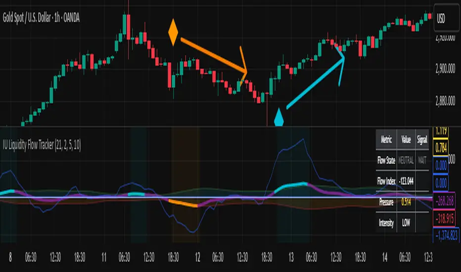
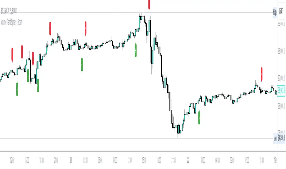
Adaptivity: Measures of Dominant Cycles and Price Trend [Loxx]Adaptivity: Measures of Dominant Cycles and Price Trend is an indicator that outputs adaptive lengths using various methods for dominant cycle and price trend timeframe adaptivity. While the information output from this indicator might be useful for the average trader in one off circumstances, this indicator is really meant for those need a quick comparison of dynamic length outputs who wish to fine turn algorithms and/or create adaptive indicators.
This indicator compares adaptive output lengths of all publicly known adaptive measures. Additional adaptive measures will be added as they are discovered and made public.
The first released of this indicator includes 6 measures. An additional three measures will be added with updates. Please check back regularly for new measures.
Ehers:
Autocorrelation Periodogram
Band-pass
Instantaneous Cycle
Hilbert Transformer
Dual Differentiator
Phase Accumulation (future release)
Homodyne (future release)
Jurik:
Composite Fractal Behavior (CFB)
Adam White:
Veritical Horizontal Filter (VHF) (future release)
What is an adaptive cycle, and what is Ehlers Autocorrelation Periodogram Algorithm?
From his Ehlers' book Cycle Analytics for Traders Advanced Technical Trading Concepts by John F. Ehlers , 2013, page 135:
"Adaptive filters can have several different meanings. For example, Perry Kaufman's adaptive moving average (KAMA) and Tushar Chande's variable index dynamic average (VIDYA) adapt to changes in volatility . By definition, these filters are reactive to price changes, and therefore they close the barn door after the horse is gone.The adaptive filters discussed in this chapter are the familiar Stochastic , relative strength index (RSI), commodity channel index (CCI), and band-pass filter.The key parameter in each case is the look-back period used to calculate the indicator. This look-back period is commonly a fixed value. However, since the measured cycle period is changing, it makes sense to adapt these indicators to the measured cycle period. When tradable market cycles are observed, they tend to persist for a short while.Therefore, by tuning the indicators to the measure cycle period they are optimized for current conditions and can even have predictive characteristics.
The dominant cycle period is measured using the Autocorrelation Periodogram Algorithm. That dominant cycle dynamically sets the look-back period for the indicators. I employ my own streamlined computation for the indicators that provide smoother and easier to interpret outputs than traditional methods. Further, the indicator codes have been modified to remove the effects of spectral dilation.This basically creates a whole new set of indicators for your trading arsenal."
What is this Hilbert Transformer?
An analytic signal allows for time-variable parameters and is a generalization of the phasor concept, which is restricted to time-invariant amplitude, phase, and frequency. The analytic representation of a real-valued function or signal facilitates many mathematical manipulations of the signal. For example, computing the phase of a signal or the power in the wave is much simpler using analytic signals.
The Hilbert transformer is the technique to create an analytic signal from a real one. The conventional Hilbert transformer is theoretically an infinite-length FIR filter. Even when the filter length is truncated to a useful but finite length, the induced lag is far too large to make the transformer useful for trading.
From his Ehlers' book Cycle Analytics for Traders Advanced Technical Trading Concepts by John F. Ehlers , 2013, pages 186-187:
"I want to emphasize that the only reason for including this section is for completeness. Unless you are interested in research, I suggest you skip this section entirely. To further emphasize my point, do not use the code for trading. A vastly superior approach to compute the dominant cycle in the price data is the autocorrelation periodogram. The code is included because the reader may be able to capitalize on the algorithms in a way that I do not see. All the algorithms encapsulated in the code operate reasonably well on theoretical waveforms that have no noise component. My conjecture at this time is that the sample-to-sample noise simply swamps the computation of the rate change of phase, and therefore the resulting calculations to find the dominant cycle are basically worthless.The imaginary component of the Hilbert transformer cannot be smoothed as was done in the Hilbert transformer indicator because the smoothing destroys the orthogonality of the imaginary component."
What is the Dual Differentiator, a subset of Hilbert Transformer?
From his Ehlers' book Cycle Analytics for Traders Advanced Technical Trading Concepts by John F. Ehlers , 2013, page 187:
"The first algorithm to compute the dominant cycle is called the dual differentiator. In this case, the phase angle is computed from the analytic signal as the arctangent of the ratio of the imaginary component to the real component. Further, the angular frequency is defined as the rate change of phase. We can use these facts to derive the cycle period."
What is the Phase Accumulation, a subset of Hilbert Transformer?
From his Ehlers' book Cycle Analytics for Traders Advanced Technical Trading Concepts by John F. Ehlers , 2013, page 189:
"The next algorithm to compute the dominant cycle is the phase accumulation method. The phase accumulation method of computing the dominant cycle is perhaps the easiest to comprehend. In this technique, we measure the phase at each sample by taking the arctangent of the ratio of the quadrature component to the in-phase component. A delta phase is generated by taking the difference of the phase between successive samples. At each sample we can then look backwards, adding up the delta phases.When the sum of the delta phases reaches 360 degrees, we must have passed through one full cycle, on average.The process is repeated for each new sample.
The phase accumulation method of cycle measurement always uses one full cycle's worth of historical data.This is both an advantage and a disadvantage.The advantage is the lag in obtaining the answer scales directly with the cycle period.That is, the measurement of a short cycle period has less lag than the measurement of a longer cycle period. However, the number of samples used in making the measurement means the averaging period is variable with cycle period. longer averaging reduces the noise level compared to the signal.Therefore, shorter cycle periods necessarily have a higher out- put signal-to-noise ratio."
What is the Homodyne, a subset of Hilbert Transformer?
From his Ehlers' book Cycle Analytics for Traders Advanced Technical Trading Concepts by John F. Ehlers , 2013, page 192:
"The third algorithm for computing the dominant cycle is the homodyne approach. Homodyne means the signal is multiplied by itself. More precisely, we want to multiply the signal of the current bar with the complex value of the signal one bar ago. The complex conjugate is, by definition, a complex number whose sign of the imaginary component has been reversed."
What is the Instantaneous Cycle?
The Instantaneous Cycle Period Measurement was authored by John Ehlers; it is built upon his Hilbert Transform Indicator.
From his Ehlers' book Cybernetic Analysis for Stocks and Futures: Cutting-Edge DSP Technology to Improve Your Trading by John F. Ehlers, 2004, page 107:
"It is obvious that cycles exist in the market. They can be found on any chart by the most casual observer. What is not so clear is how to identify those cycles in real time and how to take advantage of their existence. When Welles Wilder first introduced the relative strength index (rsi), I was curious as to why he selected 14 bars as the basis of his calculations. I reasoned that if i knew the correct market conditions, then i could make indicators such as the rsi adaptive to those conditions. Cycles were the answer. I knew cycles could be measured. Once i had the cyclic measurement, a host of automatically adaptive indicators could follow.
Measurement of market cycles is not easy. The signal-to-noise ratio is often very low, making measurement difficult even using a good measurement technique. Additionally, the measurements theoretically involve simultaneously solving a triple infinity of parameter values. The parameters required for the general solutions were frequency, amplitude, and phase. Some standard engineering tools, like fast fourier transforms (ffs), are simply not appropriate for measuring market cycles because ffts cannot simultaneously meet the stationarity constraints and produce results with reasonable resolution. Therefore i introduced maximum entropy spectral analysis (mesa) for the measurement of market cycles. This approach, originally developed to interpret seismographic information for oil exploration, produces high-resolution outputs with an exceptionally short amount of information. A short data length improves the probability of having nearly stationary data. Stationary data means that frequency and amplitude are constant over the length of the data. I noticed over the years that the cycles were ephemeral. Their periods would be continuously increasing and decreasing. Their amplitudes also were changing, giving variable signal-to-noise ratio conditions. Although all this is going on with the cyclic components, the enduring characteristic is that generally only one tradable cycle at a time is present for the data set being used. I prefer the term dominant cycle to denote that one component. The assumption that there is only one cycle in the data collapses the difficulty of the measurement process dramatically."
What is the Band-pass Cycle?
From his Ehlers' book Cycle Analytics for Traders Advanced Technical Trading Concepts by John F. Ehlers , 2013, page 47:
"Perhaps the least appreciated and most underutilized filter in technical analysis is the band-pass filter. The band-pass filter simultaneously diminishes the amplitude at low frequencies, qualifying it as a detrender, and diminishes the amplitude at high frequencies, qualifying it as a data smoother. It passes only those frequency components from input to output in which the trader is interested. The filtering produced by a band-pass filter is superior because the rejection in the stop bands is related to its bandwidth. The degree of rejection of undesired frequency components is called selectivity. The band-stop filter is the dual of the band-pass filter. It rejects a band of frequency components as a notch at the output and passes all other frequency components virtually unattenuated. Since the bandwidth of the deep rejection in the notch is relatively narrow and since the spectrum of market cycles is relatively broad due to systemic noise, the band-stop filter has little application in trading."
From his Ehlers' book Cycle Analytics for Traders Advanced Technical Trading Concepts by John F. Ehlers , 2013, page 59:
"The band-pass filter can be used as a relatively simple measurement of the dominant cycle. A cycle is complete when the waveform crosses zero two times from the last zero crossing. Therefore, each successive zero crossing of the indicator marks a half cycle period. We can establish the dominant cycle period as twice the spacing between successive zero crossings."
What is Composite Fractal Behavior (CFB)?
All around you mechanisms adjust themselves to their environment. From simple thermostats that react to air temperature to computer chips in modern cars that respond to changes in engine temperature, r.p.m.'s, torque, and throttle position. It was only a matter of time before fast desktop computers applied the mathematics of self-adjustment to systems that trade the financial markets.
Unlike basic systems with fixed formulas, an adaptive system adjusts its own equations. For example, start with a basic channel breakout system that uses the highest closing price of the last N bars as a threshold for detecting breakouts on the up side. An adaptive and improved version of this system would adjust N according to market conditions, such as momentum, price volatility or acceleration.
Since many systems are based directly or indirectly on cycles, another useful measure of market condition is the periodic length of a price chart's dominant cycle, (DC), that cycle with the greatest influence on price action.
The utility of this new DC measure was noted by author Murray Ruggiero in the January '96 issue of Futures Magazine. In it. Mr. Ruggiero used it to adaptive adjust the value of N in a channel breakout system. He then simulated trading 15 years of D-Mark futures in order to compare its performance to a similar system that had a fixed optimal value of N. The adaptive version produced 20% more profit!
This DC index utilized the popular MESA algorithm (a formulation by John Ehlers adapted from Burg's maximum entropy algorithm, MEM). Unfortunately, the DC approach is problematic when the market has no real dominant cycle momentum, because the mathematics will produce a value whether or not one actually exists! Therefore, we developed a proprietary indicator that does not presuppose the presence of market cycles. It's called CFB (Composite Fractal Behavior) and it works well whether or not the market is cyclic.
CFB examines price action for a particular fractal pattern, categorizes them by size, and then outputs a composite fractal size index. This index is smooth, timely and accurate
Essentially, CFB reveals the length of the market's trending action time frame. Long trending activity produces a large CFB index and short choppy action produces a small index value. Investors have found many applications for CFB which involve scaling other existing technical indicators adaptively, on a bar-to-bar basis.
What is VHF Adaptive Cycle?
Vertical Horizontal Filter (VHF) was created by Adam White to identify trending and ranging markets. VHF measures the level of trend activity, similar to ADX DI. Vertical Horizontal Filter does not, itself, generate trading signals, but determines whether signals are taken from trend or momentum indicators. Using this trend information, one is then able to derive an average cycle length.
Komut dosyalarını "accumulation" için ara
Market PulseBINANCE:BTCUSDT
This is the "Market Pulse" indicator from TOS Indicators.
The scope of this indicator is to identify which one of the four market stages we're in
█ WHAT ARE THE 4 STAGES?
ACCELERATION (or uptrend)
DECELERATION (or downtrend)
ACCUMULATION (occurs after the market has presumably found a bottom and buyers are coming in)
DISTRIBUTION (occurs after the market has presumably found a top and sellers are coming in)
█ WHAT ARE THE TOOLS THAT IT USES TO IDENTIFY THEM?
3 VWMA (Volume Weighted Moving Average)
1 VMA (Variable Moving Average)
VWMA = is a moving average which takes volume into account, and gives closes with higher volume an higher weight
vwma(src, len) => ta.sma(src * volume, len) / ta.sma(volume, len)
VMA = is a moving average which automatically adjusts the smoothing constant using Market Volatility
vma(src, len) =>
vi = ta.cmo(src, len) / 100
alpha = 2 / (len + 1) * math.abs(vi)
vma = 0.0
vma := alpha * src + nz(vma ) * (1 - alpha)
█ HOW CAN I INTERPRET THE INDICATOR?
1) On the top right you can see a box which tells you the Market Stage of the chart you are currently using:
If VWMA8 > VWMA21 > VWMA34 it signals ACCELERATION, color coded in green
If VWMA8 < VWMA21 < VWMA34 it signals DECELERATION, color coded in red
If neither of the previous two conditions are met it signals ACCUMULATION (yellow) if price closes above the VMA and DISTRIBUTION (orange) if price closes below the VMA
2) Next you have the actual VMA which is the line plotted on the chart and color coded in green, red or gray accordingly to the Market Stage with a filter applied:
for a bullish signal (green label) the market needs to be in ACCELERATION and price must be above the VMA
for a bearish signal (red label) the market needs to be in DECELERATION and price must be below the VMA
This characteristic makes it sometimes slower at giving direction indications, but also makes it more suitable to be considered as actual signals for buying and selling
ACCUMULATION and DISTRIBUTION are both rapresented with color gray, if you want you can consider:
the line going from green to gray as ACCUMULATION, your bias is bullish until the line turns red
the line going from red to gray as DISTRIBUTION, your bias is bearish until the line turns green
3) Then you can choose to plot the 3 VWMA to indentify pullbacks and entries for your trades
4) Finally you have the Market Screener, which you can choose to plot and gives a fast look to the markets you are interested on
It basically gives you the Market Stage for every Symbol you choose using the timeframes you input
The maximum number of Symbols you can set is 20, and for all of them you have 2 different timeframes you can choose to analyse.
By default the Symbols are set to the top 20 Cryptocurrency by Market Cap, and the timeframes to 4h and D
There is an option which is on by default and color codes ACCUMULATION and DISTRIBUTION the same as the box on the top right, you can turn it off to make them gray
As I've written in the tooltip inside the indicator you should only use the screener to analyse timeframes which are equal or higher than the one you are currently on your chart.
If you don't plan to use the screener you can delete every symbol from the input boxes to make the indicator update faster when changing timeframe or market.
Be aware that the screener is on BETA and may give repainting signals!
Volume Range Profile with Fair Value (Zeiierman)█ Overview
The Volume Range Profile with Fair Value (Zeiierman) is a precision-built volume-mapping tool designed to help traders visualize where institutional-level activity is occurring within the price range — and how that volume behavior shifts over time.
Unlike traditional volume profiles that rely on fixed session boundaries or static anchors, this tool dynamically calculates and displays volume zones across both the upper and lower ends of a price range, revealing point-of-control (POC) levels, directional volume flow, and a fair value drift line that updates live with each candle.
You’re not just looking at volume anymore. You’re dissecting who’s in control — and at what price.
⚪ In simple terms:
Upper Zone = The upper portion of the price range, showing concentrated volume activity — typically where selling or distribution may occur
Lower Zone = The lower portion of the price range, highlighting areas of high volume — often associated with buying or accumulation
POC Bin = The bin (price level) with the highest traded volume in the zone — considered the most accepted price by the market
Fair Value Trend = A dynamic trend line tracking the average POC price over time — visualizing the evolving fair value
Zone Labels = Display real-time breakdown of buy/sell volume within each zone and inside the POC — revealing who’s in control
█ How It Works
⚪ Volume Zones
Upper Zone: Anchored at the highest high in the lookback period
Lower Zone: Anchored at the lowest low in the lookback period
Width is user-defined via % of range
Each zone is divided into a series of volume bins
⚪ Volume Bins (Histograms)
Each zone is split into N bins that show how much volume occurred at each level:
Taller = More volume
The POC bin (Point of Control) is highlighted
Labels show % of volume in the POC relative to the whole zone
⚪ Buy vs Sell Breakdown
Each volume bin is split by:
Buy Volume = Close ≥ Open
Sell Volume = Close < Open
The script accumulates these and displays total Buy/Sell volume per zone.
⚪ Fair Value Drift Line
A POC trend is plotted over time:
Represents where volume was most active across each range
Color changes dynamically — green for rising, red for falling
Serves as a real-time fair value anchor across changing market structure
█ How to Use
⚪ Identify Key Control Zones
Use Upper/Lower Zone structures to understand where supply and demand is building.
Zones automatically adapt to recent highs/lows and re-center volume accordingly.
⚪ Follow Institutional Activity
Watch for POC clustering near price tops or bottoms.
Large volumes near extremes may indicate accumulation or distribution.
⚪ Spot Fair Value Drift
The fair value trend line (average POC price) gives insight into market equilibrium.
One strategy can be to trade a re-test of the fair value trend, trades are taken in the direction of the current trend.
█ Understanding Buy & Sell Volume Labels (Zone Totals)
These labels show the total buy and sell volume accumulated within each zone over the selected lookback period:
Buy Vol (green label) → Total volume where candles closed bullish
Sell Vol (red label) → Total volume where candles closed bearish
Together, they tell you which side dominated:
Higher Buy Vol → Bullish accumulation zone
Higher Sell Vol → Bearish distribution zone
This gives a quick visual insight into who controlled the zone, helping you spot areas of demand or supply imbalance.
█ Understanding POC Volume Labels
The POC (Point of Control) represents the price level where the most volume occurred within the zone. These labels break down that volume into:
Buy % – How much of the volume was buying (price closed up)
Sell % – How much was selling (price closed down)
Total % – How much of the entire zone’s volume happened at the POC
Use it to spot strong demand or supply zones:
High Buy % + High Total % → Strong buying interest = likely support
High Sell % + High Total % → Strong selling pressure = likely resistance
It gives a deeper look into who was in control at the most important price level.
█ Why It’s Useful
Track where fair value is truly forming
Detect aggressive volume accumulation or dumping
Visually split buyer/seller control at the most relevant price levels
Adapt volume structures to current trend direction
█ Settings Explained
Lookback Period: Number of bars to scan for highs/lows. Higher = smoother zones, Lower = reactive.
Zone Width (% of Range): Controls how much of the range is used to define each zone. Higher = broader zones.
Bins per Zone: Number of volume slices per zone. Higher = more detail, but heavier on resources.
-----------------
Disclaimer
The content provided in my scripts, indicators, ideas, algorithms, and systems is for educational and informational purposes only. It does not constitute financial advice, investment recommendations, or a solicitation to buy or sell any financial instruments. I will not accept liability for any loss or damage, including without limitation any loss of profit, which may arise directly or indirectly from the use of or reliance on such information.
All investments involve risk, and the past performance of a security, industry, sector, market, financial product, trading strategy, backtest, or individual's trading does not guarantee future results or returns. Investors are fully responsible for any investment decisions they make. Such decisions should be based solely on an evaluation of their financial circumstances, investment objectives, risk tolerance, and liquidity needs.
Grid TraderGrid Trader Indicator ( GTx ):
Overview
The Grid Trader Indicator is a tool that helps traders visualize key levels within a specified trading range. The indicator plots accumulation and distribution levels, an entry level, an exit level, and a midpoint. This guide will help you understand how to use the indicator and its features for effective grid trading.
Basics of Trading Range, Grid Buy, and Grid Sell
Trading Range
A trading range is the horizontal price movement between a defined upper ( resistance ) and lower ( support ) level over a period of time. When a security trades within a range, it repeatedly moves between these two levels without trending upwards or downwards significantly. Traders often use the trading range to identify potential buy and sell points:
Upper Level (Resistance): This is the price level at which selling pressure overcomes buying pressure, preventing the price from rising further.
Lower Level (Support): This is the price level at which buying pressure overcomes selling pressure, preventing the price from falling further.
Grid Trading Strategy
Grid trading is a type of trading strategy that involves placing buy and sell orders at predefined intervals around a set price. It aims to profit from the natural market volatility by buying low and selling high in a range-bound market. The strategy divides the trading range into several grid levels where orders are placed.
Grid Buy
Grid buy orders are placed at intervals below the current price . When the price drops to these levels, buy orders are triggered . This strategy ensures that the trader buys more as the price falls, potentially lowering the average purchase price .
Grid Sell
Grid sell orders are placed at intervals above the current price . When the price rises to these levels, sell orders are triggered . This ensures that the trader sells portions of their holdings as the price increases, potentially securing profits at higher levels .
Key Points of Grid Trading
Grid Size : The interval between each buy and sell order. This can be constant (e.g., $2 intervals) or variable based on certain conditions.
Accumulation Range : The lower part of the trading range where buy orders are placed.
Distribution Range : The upper part of the trading range where sell orders are placed.
Midpoint : The average price of the entry and exit levels, often used as a reference point for balance.
As the price moves up and down within this range, your buy orders will be triggered as the price drops and your sell orders will be triggered as the price rises. This allows you to accumulate more of the asset at lower prices and sell portions at higher prices, profiting from the price oscillations within the defined range. Grid trading can be particularly effective in a sideways market where there is no clear long-term trend. However, it requires careful monitoring and adjustment of grid levels based on market conditions to minimize risks and maximize returns .
Configuring the Indicator :
Once the indicator is added, you will see a settings icon next to it. Click on it to open the settings menu.
Adjust the Upper Level , Lower Level , Entry Level , and Exit Level to match your trading strategy and market conditions.
Set the Levels Visibility to control how many bars back the levels will be plotted.
Interpreting the Levels :
Accumulation Levels : These are plotted below the entry level and are potential buy zones. They are labeled as Accumulation Level 1, 2, and 3.
Distribution Levels : These are plotted above the exit level and are potential sell zones. They are labeled as Distribution Level 1, 2, and 3.
Upper Level : Marked in fuchsia, indicating the top boundary of the trading range.
Exit Level : Marked in yellow, indicating the level at which you plan to exit trades.
Midpoint : Marked in white, indicating the average of the entry and exit levels.
Entry Level : Marked in yellow, indicating the level at which you plan to enter trades.
Lower Level : Marked in aqua, indicating the bottom boundary of the trading range.
By visualizing key levels, you can make informed decisions on where to place buy and sell orders, potentially maximizing your trading profits through systematic grid trading.
Sadgir Patterns with SL/TPThe "Sadgir Patterns with SL/TP" is a cutting-edge trading indicator designed for traders seeking to leverage the power of Hull Moving Averages in conjunction with phase accumulation analysis. This unique indicator, developed on the Pine Script platform, is ideal for various markets, including stocks, forex, cryptocurrencies, and commodities.
Key Features:
Adaptive Hull Moving Average: Utilizes an adaptive Hull Moving Average, which provides a smooth and responsive moving average line, aiding in identifying trend directions and potential market reversals.
Phase Accumulation Analysis: Integrates phase accumulation calculations to dynamically adjust the length of the Hull Moving Average, ensuring that the indicator stays in sync with market conditions.
Signal Generation: Generates clear "Long" and "Short" signals, which are visually represented on the chart, assisting traders in making informed decisions.
Dynamic Stop Loss and Take Profit Levels: Automatically calculates and plots dynamic stop loss (SL) and take profit (TP) levels as horizontal lines on the chart, based on user-defined percentage settings. These levels adjust in real-time with the price action, offering a systematic approach to risk management.
Customizable Settings: Provides users with the flexibility to adjust the source of the moving average, power settings for the Hull Moving Average, cycles, and powers for phase accumulation, as well as the percentage values for SL and TP levels.
Visual and Alert Features: Includes options for coloring the bars based on the trend direction and displays trade signals with distinct shapes. Additionally, alert conditions are set for both Long and Short signals, enabling traders to stay informed of potential trade opportunities.
Usage:
This indicator is designed for traders of all levels, from beginners to advanced. It can be used for trend following, catching reversals, or as part of a larger trading strategy. The dynamic SL and TP levels aid in managing trades effectively, providing both entry and exit points. However, traders are advised to use this indicator in conjunction with other analysis tools and consider the overall market context for the best results.
Disclaimer:
Trading involves risk, and it's important to do your own research and consider your risk tolerance before using this indicator. This tool is not intended as financial advice.
NSE:BANKNIFTY
NSE:NIFTY
MCX:CRUDEOIL1!
Market Phases NJRMarket Phases Indicator
Overview:
The Market Phases Indicator is a versatile tool designed for traders to identify key market phases, including accumulation, distribution, markup, and markdown. By analyzing the relationship between price and volume, this indicator aims to assist traders in recognizing potential shifts in market sentiment and trend direction.
Features:
1. **Moving Average Analysis:**
- Utilizes a customizable moving average length to assess the overall trend direction.
2. **Volume Confirmation:**
- Incorporates volume analysis to confirm the strength of identified market phases.
3. **Visualization:**
- Clearly visualizes accumulation, distribution, markup, and markdown phases on the price chart using intuitive shapes.
Input Parameters:
- **Moving Average Length (default: 20):**
- Adjusts the length of the moving average for trend analysis.
- **Volume Multiplier (default: 1.5):**
- Sets the multiplier to customize the volume threshold for identifying significant market phases.
How to Use:
1. **Accumulation and Distribution:**
- Green triangles indicate potential accumulation phases when the closing price is above the moving average, and volume is higher than the specified threshold. Red triangles indicate potential distribution phases.
2. **Markup and Markdown:**
- Blue triangles suggest potential markup phases when the closing price is above the moving average, and volume is below the specified threshold. Orange triangles indicate potential markdown phases.
Important Notes:
- This indicator is a tool for analysis and should be used in conjunction with other technical analysis methods.
- Parameters can be adjusted based on the specific characteristics of the asset being analyzed.
Disclaimer:
Trading involves risk, and no indicator can guarantee profits. Users should exercise caution, conduct thorough research, and consider risk management principles when making trading decisions.
PA-Adaptive T3 Loxxer [Loxx]PA-Adaptive T3 Loxxer is a Loxxer indicator that is Phase Accumulation Cycle adaptive and uses T3 moving average for smoothing instead of the typical SMA or EMA . this allows for smoother signals by reducing noise.
What is Loxxer?
The Loxxer indicator is a technical analysis tool that compares the most recent maximum and minimum prices to the previous period's equivalent price to measure the demand of the underlying asset.
What is the Phase Accumulation Cycle?
The phase accumulation method of computing the dominant cycle is perhaps the easiest to comprehend. In this technique, we measure the phase at each sample by taking the arctangent of the ratio of the quadrature component to the in-phase component. A delta phase is generated by taking the difference of the phase between successive samples. At each sample we can then look backwards, adding up the delta phases.When the sum of the delta phases reaches 360 degrees, we must have passed through one full cycle, on average.The process is repeated for each new sample.
The phase accumulation method of cycle measurement always uses one full cycle’s worth of historical data.This is both an advantage and a disadvantage.The advantage is the lag in obtaining the answer scales directly with the cycle period.That is, the measurement of a short cycle period has less lag than the measurement of a longer cycle period. However, the number of samples used in making the measurement means the averaging period is variable with cycle period. longer averaging reduces the noise level compared to the signal.Therefore, shorter cycle periods necessarily have a higher out- put signal-to-noise ratio.
Included
Bar coloring
Signals
Alerts
Loxx's Expanded Source Types
Divergences
[blackcat] L3 Banker Fund AttackLevel 3
Background
This indicator is used to capture the movement of the banker fund. The buying and selling point is determined according to whether the momentum of the banker fund and the price momentum resonate.
How to use the indicator:
The red column line indicates that the banker fund accumulation signal appears, and the following 2 conditions are all satisfied to buy; (both above the green line of the banker fund attack threshold)
1. The yellow line and the purple line all cross the red accumulation histogram signal;
2. The yellow and purple trend lines are up
Key point: If the yellow line crosses the green line of the banker fund attack threshold, it will be pulled up or the big market will open! The main thing is to see the red accumulation histogram signal, or the green line that crosses the banker fund attack threshold. If there is a red accumulation histogram signal, it means that there are main low-acquisition chips, and start trading on the left to open a position. The area above the green line of the banker fund attack threshold belongs to the main force pulling stage. When the green line of the banker fund attack threshold is not broken upwards, there is still a lot of profit space, but if it can be effectively broken through, it is highly profitable!
Remarks
This indicator only effective for instruments that contains banker fund. If there is no obvious large fund inside, the indicator is not as meaningful as it is called.
I verified it worked well for > 4H or 1D timeframe. For the other time frames, you may need to check and verify by yourself.
Feedbacks are appreciated.
PA-Adaptive Polynomial Regression Fitted Moving Average [Loxx]PA-Adaptive Polynomial Regression Fitted Moving Average is a moving average that is calculated using Polynomial Regression Analysis. The purpose of this indicator is to introduce polynomial fitting that is to be used in future indicators. This indicator also has Phase Accumulation adaptive period inputs. Even though this first indicator is for demonstration purposes only, its still one of the only viable implementations of Polynomial Regression Analysis on TradingView is suitable for trading, and while this same method can be used to project prices forward, I won't be doing that since forecasting is generally worthless and causes unavoidable repainting. This indicator only repaints on the current bar. Once the bar closes, any signal on that bar won't change.
For other similar Polynomial Regression Fitted methodologies, see here
Poly Cycle
What is the Phase Accumulation Cycle?
The phase accumulation method of computing the dominant cycle is perhaps the easiest to comprehend. In this technique, we measure the phase at each sample by taking the arctangent of the ratio of the quadrature component to the in-phase component. A delta phase is generated by taking the difference of the phase between successive samples. At each sample we can then look backwards, adding up the delta phases.When the sum of the delta phases reaches 360 degrees, we must have passed through one full cycle, on average.The process is repeated for each new sample.
The phase accumulation method of cycle measurement always uses one full cycle’s worth of historical data.This is both an advantage and a disadvantage.The advantage is the lag in obtaining the answer scales directly with the cycle period.That is, the measurement of a short cycle period has less lag than the measurement of a longer cycle period. However, the number of samples used in making the measurement means the averaging period is variable with cycle period. longer averaging reduces the noise level compared to the signal.Therefore, shorter cycle periods necessarily have a higher out- put signal-to-noise ratio.
What is Polynomial Regression?
In statistics, polynomial regression is a form of regression analysis in which the relationship between the independent variable x and the dependent variable y is modelled as an nth degree polynomial in x. Polynomial regression fits a nonlinear relationship between the value of x and the corresponding conditional mean of y, denoted E(y |x). Although polynomial regression fits a nonlinear model to the data, as a statistical estimation problem it is linear, in the sense that the regression function E(y | x) is linear in the unknown parameters that are estimated from the data. For this reason, polynomial regression is considered to be a special case of multiple linear regression.
Things to know
You can select from 33 source types
The source is smoothed before being injected into the Polynomial fitting algorithm, there are 35+ moving averages to choose from for smoothing
The output of the Polynomial fitting algorithm is then smoothed to create the signal, there are 35+ moving averages to choose from for smoothing
Included
Alerts
Signals
Bar coloring
PA-Adaptive TRIX Log [Loxx]PA-Adaptive TRIX Log is a Phase Accumulation Adaptive TRIX Log indicator. This adaptation smooths the signal to catch larger trends.
What is TRIX?
TRIX is a momentum oscillator that displays the percent rate of change of a TEMA . It was developed in the early 1980's by Jack Hutson, an editor for "Technical Analysis of Stocks and Commodities" magazine. With its triple smoothing, TRIX is designed to filter insignificant price movements. In his article he uses a logarithm of a price (which is in many versions, left out).
What is the Phase Accumulation Cycle?
The phase accumulation method of computing the dominant cycle is perhaps the easiest to comprehend. In this technique, we measure the phase at each sample by taking the arctangent of the ratio of the quadrature component to the in-phase component. A delta phase is generated by taking the difference of the phase between successive samples. At each sample we can then look backwards, adding up the delta phases.When the sum of the delta phases reaches 360 degrees, we must have passed through one full cycle, on average.The process is repeated for each new sample.
The phase accumulation method of cycle measurement always uses one full cycle’s worth of historical data.This is both an advantage and a disadvantage.The advantage is the lag in obtaining the answer scales directly with the cycle period.That is, the measurement of a short cycle period has less lag than the measurement of a longer cycle period. However, the number of samples used in making the measurement means the averaging period is variable with cycle period. longer averaging reduces the noise level compared to the signal.Therefore, shorter cycle periods necessarily have a higher out- put signal-to-noise ratio.
Included
Bar coloring
2 signal options
Alerts
Volume Indicators PackageCONTAINS 3 OF MY BEST VOLUME INDICATORS ALL FOR THE PRICE OF ONE!
CONTAINS:
Average Dollar Volume in RED
Up/Down Volume Ratio in Green
Volume Buzz/Volume Run Rate in BLUE
If you would like to get these individually, I also have scripts for that too.
Below is information about all three of these indicators, what they do, and why they are important.
---------------------------------------------------------------------------------------------AVERAGE DOLLAR VOLUME----------------------------------------------------------------------------------------
Dollar volume is simply the volume traded multiplied times the cost of the stock.
Dollar volume is an extremely important metric for finding stocks with enough liquidity for market makers to position themselves in. Market Liquidity is defined as market's feature whereby an individual or firm can quickly purchase or sell an asset without causing a drastic change in the asset's price. The key concept you want to understand is that these big instructions with billions of dollars need liquidity in a stock in order to even think about buying it, and therefore these institutions will demand a large dollar volume . A good dollar volume amount, that represents a pretty liquid name, is typically above 100 million $ average. Why are institutions important? Simple because they are the ones who make stocks move, and I mean really move. If you want to see large growth from a stock in a short amount of time, you need institutions wielding billions of dollars to be fighting one another to buy more shares. Institutions are the ones who make or break a stock, this is why we call them market makers.
My script calculates average dollar volume using four averages: the 50, the 30, the 20, and the 10 period. I use multiple averages in order to provide the accurate and up to date information to you. It then selects the minimum of these averages and divides this value by 1 million and displays this number to you.
TL;DR? If you want monster moves from your stocks, you need to pick names with average high liquidity(dollar volume >= $100 million). The number presented to you is in millions of whatever currency the name is traded in.
---------------------------------------------------------------------------------------------UP/DOWN VOLUME RATIO-----------------------------------------------------------------------------------------
Up/Down Volume Ratio is calculated by summing volume on days when it closes up and divide that total by the volume on days when the stock closed down.
High volume up days are typically a sign of accumulation(buying) by big players, while down days are signs of distribution(selling) by big market players. The Up Down volume ratio takes this assumption and turns it into a tangible number that's easier for the trader to understand. My formula is calculated using the past 50 periods, be warned it will not display a value for stocks with under 50 periods of trading history. This indicator is great for identify accumulation of growth stocks early on in their moves, most of the time you would like a growth stocks U/D value to be above 2, showing institutional sponsorship of a stock.
Up/Down Volume value interpretation:
U/D < 1 -> Bearish outlook, as sellers are in control
U/D = 1 -> Sellers and Buyers are equal
U/D > 1 -> Bullish outlook, as buyers are in control
U/D > 2 -> Bullish outlook, significant accumulation underway by market makers
U/D >= 3 -> MONSTER STOCK ALERT, market makers can not get enough of this stock and are ravenous to buy more
U/D values greater than 2 are rare and typically do not last very long, and U/D >= 3 are extremely rare one example I kind find of a stock's U/D peaking above 3 was Google back in 2005.
-----------------------------------------------------------------------------------------------------VOLUME BUZZ-----------------------------------------------------------------------------------------------
Volume Buzz/ Volume Run Rate as seen on TC2000 and MarketSmith respectively.
Basically, the volume buzz tells you what percentage over average(100 time period moving average) the volume traded was. You can use this indicator to more readily identify above-average trading volume and accumulation days on charts. The percentage will show up in the top left corner, make sure to click the settings button and uncheck the second box(left of plot) in order to get rid of the chart line.
Dynamic Money FlowDynamic Money Flow is a volume indicator based on Marc Chaikin's Money Flow with a few improvements.
It can be used to confirm break-outs and trends.
Zero line crosses and divergences can provide useful signals while considering chart analysis as well.
Two weaknesses of CMF have been already fixed by Colin Twiggs (IncredibleCharts)...
1.CMF uses Chaikin's accumulation/distribution line to calculate the flow of money.
Accumulation/distribution line does not take the gaps into account. This can be solved using true range.
I call it true accumulation/distribution.
2.Oscillators have a tendency to center because of averaging calculations.
DMF is average of flowing volume divided by average of total volume. This means indicator plots the change of first factor compared to the other one. In Simple Averaging method every data is given an equal weight thus when the last data drops it will have heavy impact on the averages and the change of them.
It is much easier to identity these impacts after the drop of very high or very low data... So reducing the weight exponentially is a better option.
3.There is something else with CMF... changes of close price is ignored, because the formula only compares close price to its range.
To include the movements of close beside the close to range comparison, the distance between two last close prices should be compared to true range as well.
So volume can be distributed between close to range comparison (True Accumulation/Distribution) and close to close comparison automatically. And then results are summed to have a single multiplier.
An example for how close to close comparison affects DMF...
Or here you can see how lower wicks keep TMF (same as CMF in this case) from crossing zero line while price is trending down.
BK AK-SILENCER🚨 Introducing BK AK-SILENCER — Volume Footprint Warfare, Right on the Price Bars 🚨
This isn’t a traditional indicator.
This is a tactical weapon — engineered to expose institutional behavior directly in the bar data, using volume logic, CVD divergence, and spike detection to pinpoint who’s really in control of the tape.
No panels. No clutter.
Just silent execution — built directly into price itself.
🔥 Why "SILENCER"?
Because real power moves in silence.
Institutions don’t chase — they build positions quietly, in size, beneath the surface.
BK AK-SILENCER gives you a real-time edge by visually revealing their footprints through color-coded bar behavior, divergence signals, and volume spike alerts — all directly on your chart.
🔹 “AK” honors my mentor A.K., whose training forged my trading discipline.
🔹 “SILENCER” represents the institutional mindset — high impact, low visibility. This tool lets you trade like them: without noise, without hesitation, with deadly clarity.
🧠 What Is BK AK-SILENCER?
A bar-level institutional detection tool, purpose-built to:
✅ Color-code bars based on volume aggression and close-location inside range
✅ Detect real-time bullish and bearish divergences between price and volume delta
✅ Tag volume spikes with a $ symbol to expose potential traps or silent position builds
✅ Overlay VWAP for real-time mean-reversion biasing
No extra windows.
No indicators talking over each other.
Just pure volume-logic weaponry embedded into price.
⚙️ What This Weapon Deploys
🔸 Bar Coloring Logic (Volume Footprint)
🟢 Power Buy = Strong close near highs on elevated volume
🟩 Accumulation = Weak close but still heavy volume
🔴 Power Sell = Strong close near lows on heavy selling
🟥 Distribution / Weakness = Low close without commitment
❗ Extreme Volume Spikes marked with $ — using standard deviation to highlight institutional bursts
🔸 CVD Divergence Detection
→ Tracks cumulative volume delta and compares it to price pivot behavior
Bullish Divergence = Price makes lower lows, CVD makes higher lows → hidden accumulation
Bearish Divergence = Price makes higher highs, CVD makes lower highs → hidden distribution
All plotted directly on bars with triangle markers.
🔸 VWAP Overlay (Optional)
→ Anchored VWAP gives immediate context for intraday bias — above VWAP = demand, below = supply
🎯 How to Use BK AK-SILENCER
🔹 Silent Reversal Detection
Bullish divergence + Power Buy bar + VWAP reclaim = sniper entry
Bearish divergence + Power Sell bar + VWAP rejection = trap confirmation
🔹 Volume-Based Entry Triggers
Look for Power Buy + $ spike after a pullback → watch for quiet reversal
Accumulation colors clustering? Institutions are likely loading silently
🔹 Institutional Trap Warnings
$ spike + red distribution bar at highs = time to exit or flip
Weakness bar below VWAP? Don’t chase the long.
🛡️ Why It Matters
✅ Clean — it integrates into price action, no separate panels
✅ Silent — tracks institutions who build without alerts or indicators
✅ Tactical — no fluff, no lag, just real-time behavior recognition
This tool is ideal for:
🔸 Scalpers reading bar-by-bar
🔸 Intraday swing traders using VWAP and structure
🔸 Professionals who need volume behavior decoded in real-time
🔸 Anyone who wants signal without clutter
🙏 Final Thoughts
This tool isn’t just about trading — it’s about tactical awareness.
🔹 Dedicated to my mentor A.K., whose wisdom runs deep in every logic tree.
🔹 Above all, I give thanks to Gd, the source of clarity, courage, and conviction.
Without Him, even the sharpest system is blind.
With Him, we execute with structure, purpose, and divine alignment.
⚡ No noise. No clutter. No delay. Just raw, silent execution.
🔥 BK AK-SILENCER — Bar-Level Volume Footprint Precision 🔥
Gd bless every step you take in this market.
Trade with clarity, move with intention. 🙏
BTC Transaction Indicator Name: "Bitcoin On-Chain Volume & Dynamic Parabolic Curve Signals"
Purpose:
This indicator is designed for Bitcoin traders and long-term holders. It combines the analysis of Bitcoin's on-chain transaction volume with price action to generate "Whale" and "Bear" signals. Additionally, it features a unique dynamic parabolic curve that acts as a visual support line, adapting its visibility based on price interaction with a key Exponential Moving Average (EMA).
Key Components:
On-Chain Volume Analysis:
Utilizes Estimated Transaction Volume (ETRAV) data from the Bitcoin blockchain.
Calculates fast and slow Simple Moving Averages (SMAs) of this volume.
Identifies volume trends (up/down) and significant volume increases/decreases.
Employs fixed thresholds (2,500,000 for low volume and 25,000,000 for high volume) to define key activity levels, similar to how historical on-chain analysis defined accumulation and distribution zones.
Price Action Analysis:
Calculates fast and slow SMAs of the price.
Detects price trends (up/down), recoveries, and declines based on these price SMAs.
"Whale" and "Bear" Signals:
Whale Signals (Buy-side): Generated when there's an upward volume trend, significant volume increase, and a downward price trend followed by price recovery. These indicate potential accumulation phases.
Bear Signals (Sell-side): Generated when there's a downward volume trend, significant volume decrease, and an upward price trend followed by price decline. These indicate potential distribution phases.
Visuals: Both types of signals are plotted as small, colored circles directly on the price chart, with corresponding text labels ("Whale," "Buy," "Bear," "Sell," "Price Recovering," "Price Declining").
Dynamic Parabolic Curve:
Concept: A green parabolic (exponential) curve that serves as a dynamic visual support line.
Activation: The curve starts drawing automatically only when the price crosses over the EMA 500 (Exponential Moving Average of 500 periods). The curve's starting point is set at a user-defined percentage below the EMA 500 value at that exact crossover point.
Visibility: The curve remains visible and continues its trajectory only as long as the price stays above the EMA 500.
Deactivation: The curve disappears instantly if the price falls below or equals the EMA 500. It will only reappear if the price crosses above the EMA 500 again.
Customization: The curve's steepness (Tasa Crecimiento Curva) and its initial distance from the EMA 500 (Inicio Curva % por debajo de EMA500) are adjustable.
Dynamic Label: A "Parabólico" text label is plotted near the center of the active curve segment, with an adjustable vertical offset to ensure it stays visually appealing below the curve.
What is PLOTTED on the chart:
The small, colored circle signals for Whale/Buy and Bear/Sell activity.
The green dynamic parabolic curve.
What is NOT PLOTTED:
EMA 200, EMA 500 lines (though they are calculated internally for logic).
Raw volume data or volume Moving Averages (these are only used for signal calculation, not plotted).
Ideal for:
Bitcoin traders and investors focused on long-term trends and cycle analysis, who want visual cues for accumulation/distribution phases based on on-chain activity, complemented by a unique, dynamically appearing parabolic support curve.
Important Notes:
Relies on the availability of external on-chain data (QUANDL:BCHAIN) within TradingView.
Functions best on a daily timeframe for optimal on-chain data relevance.
Cycle Composite 3.6 WeightedThe Cycle Composite is a multi-factor market cycle model designed to classify long-term market behavior into distinct phases using normalized and weighted data inputs.
It combines ten key on-chain, dominance, volatility, sentiment, and trend-following metrics into a single composite output. The goal is to provide a clearer understanding of where the market may stand in the broader cycle (e.g., accumulation, early bull, late bull, or euphoria).
This version (3.4) introduces flexible weighting, trend strength markers, and additional context-aware signals such as risk-on confirmations and altseason flags.
Phases Identified:
The model categorizes the market into one of five zones:
Euphoria (> 85)
Late Bull (70 – 85)
Mid Bull (50 – 70)
Early Bull (30 – 50)
Fear (< 30)
Each phase is determined by a smoothed EMA of the weighted composite score.
Data Sources and Metrics Used (10 total):
BTC Dominance (CRYPTOCAP:BTC.D)
Stablecoin Dominance (USDT + USDC average) (inverted for risk-on)
ETH Dominance (CRYPTOCAP:ETH.D)
BBWP (normalized Bollinger Band Width % over 1-year window)
WVF (Williams VIX Fix for volatility spike detection)
NUPL (Net Unrealized Profit/Loss, external source)
CMF (Chaikin Money Flow, smoothed volume accumulation)
CEX Open Interest (custom input from DAO / external source)
Whale Inflows (custom input from whale exchange transfer data)
Google Trends Average (BTC, Crypto, Altcoin terms)
All inputs are normalized over a 200-bar window and combined via weighted averaging, where each weight is user-configurable.
Additional Features:
Phase Labels: Labels are printed only when a new phase is entered.
Bull Continuation Marker: Triangle up when composite makes higher highs and NUPL increases.
Weakening Marker: Triangle down when composite rolls over in Late Bull and NUPL falls.
Risk-On Signal: Green circle appears when CMF and Google Trends are both rising.
Altseason Flag: Orange diamond appears when dominance of "others.d" exceeds BTC.D and ETH.D and composite is above 50.
Background Shading: Each phase is shaded with a semi-transparent background color.
Timeframe-Aware Display: All markers and signals are shown only on weekly timeframe for clarity.
Intended Use:
This script is intended for educational and macro-trend analysis purposes.
It can be used to:
Identify macro cycle position (accumulation, bull phases, euphoria, etc.)
Spot long-term trend continuation or weakening signals
Add context to price action with external on-chain and sentiment data
Time rotation events such as altseason risk
Disclaimer:
This script does not constitute financial advice.
It is intended for informational and research purposes only.
Users should conduct their own due diligence and analysis before making investment decisions.
AMD Setup - Full (Long + Short) ICT ModelICTSNIPERKILLS!
Accumulation, Manipulation, Distribution (AMD) Script!
1. Clarifies Structure: Accumulation, Manipulation, Distribution (AMD)
The script visualizes the AMD framework:
Accumulation → Price ranges inside Initial Balance (IB).
Manipulation → Liquidity sweep above IB High or below IB Low.
Distribution → Market Structure Shift (MSS) confirms a directional move.
This gives you a narrative structure for each session, helping you avoid random trades.
🧠 2. Filters Out Noise with MSS Confirmation
It waits for:
A liquidity sweep (manipulation),
Followed by a market structure shift (MSS),
And then confirms an entry only after a candle closes beyond structure.
This structure:
Reduces false signals,
Improves trade timing,
Helps you align with smart money delivery.
🕘 3. Focuses on the Right Time Window (Initial Balance)
You only engage after the 10:30 AM EST close, once the Initial Balance is formed.This aligns with ICT's focus on:
Killzones (like 9:30–11:00),
Avoiding early overtrading,
Letting the market tip its hand first (through sweeps + MSS).
This timing logic supports discipline and consistency.
🟢🔴 4. Marks Entries with Risk/Reward Guidance
It plots:
AMD SHORT / LONG entries after MSS + candle confirmation,
Basic TP and SL visual markers using a static risk-reward (2:1),
Optional Fair Value Gaps (FVGs) for refinement zones.
While static, these help plan trades visually and frame targets quickly, especially if you're scalping or trading micro futures like MNQ.
📈 5. Alerts You in Real Time
Instead of manually watching:
You'll get alerts when sweeps or MSS setups appear.
You can stay focused during the killzone or walk away and return when signals trigger.
This supports patience and alert-based discipline.
💡
You already:
Use 15M/1M execution,
Wait for ERL or HOD/LOD sweeps,
Look for MSS + CISD,
Trade in killzones only,
Target 50–62–70% Fibs with SMT/FVG confluence.
This script:✅ Automates sweep + MSS detection✅ Plots AMD-based entries visually✅ Simplifies your killzone execution✅ Helps avoid FOMO by filtering setups✅ Keeps your journal entries clean with structure
BTC Growth | AlchimistOfCrypto🌈 BTC Regression Bands & Halvings – Unveiling Bitcoin's Logarithmic Growth Fields 🌈
"The Bitcoin Regression Bands, engineered through advanced logarithmic mathematics, visualizes the probabilistic distribution of Bitcoin's price evolution within a multi-cycle growth paradigm. This indicator employs principles from hyperbolic regression where decay coefficients create mathematical boundaries that define Bitcoin's long-term value progression. Our implementation features algorithmically enhanced rainbow visualization derived from extensive cycle analysis, creating a dynamic representation of Bitcoin's logarithmic growth with adaptive color gradients that highlight critical halving-based phase transitions in the asset's monetary evolution."
📊 Professional Trading Application
The Bitcoin Regression Bands transcends traditional price prediction models with a sophisticated multi-band illumination system that reveals the underlying structure of Bitcoin's monetary evolution. Scientifically calibrated across multiple halving cycles and featuring seamless rainbow visualization, it enables investors to perceive Bitcoin's position within its macro growth trajectory with unprecedented clarity.
- Visual Theming 🎨
Scientifically designed rainbow gradient optimized for cycle pattern recognition:
- Violet-Blue: Lower value accumulation zones with highest mathematical growth potential
- Green: Fair value equilibrium zone representing the regression mean
- Yellow-Orange: Moderate overvaluation regions indicating potential resistance
- Red: Statistical extreme zones indicating mathematical cycle peaks
- Halving Visualization 🔍
- Precise cycle boundaries demarcating Bitcoin's fundamental supply shock events
- Adaptive band spacing based on mathematical cycle progression
- Multiple sub-cycle markers revealing the probabilistic nature of Bitcoin's trajectory
🚀 How to Use
1. Identify Macro Position ⏰: Locate Bitcoin's current price relative to the regression bands
2. Understand Cycle Context 🎚️: Note position within the current halving cycle for time-based analysis
3. Assess Mathematical Value 🌈: Determine potential over/undervaluation based on band location
4. Adjust Investment Strategy 🔎: Modulate position sizing based on mathematical value assessment
5. Identify Cycle Phases ✅: Monitor band transitions to detect accumulation and distribution zones
6. Invest with Precision 🛡️: Utilize lower bands for strategic accumulation, upper bands for strategic reduction
7. Manage Risk Dynamically 🔐: Scale investment allocations based on mathematical cycle positioning
Money Flow Pulse💸 In markets where volatility is cheap and structure is noisy, what matters most isn’t just the move — it’s the effort behind it. Money Flow Pulse (MFP) offers a compact, color-coded readout of real-time conviction by scoring volume-weighted price action on a five-tier scale. It doesn’t try to predict reversals or validate trends. Instead, it reveals the quality of the move in progress: is it fading , driving , exhausting , or hollow ?
🎨 MFP draws from the traditional Money Flow Index (MFI), a volume-enhanced momentum oscillator, but transforms it into a modular “pressure readout” that fits seamlessly into any structural overlay. Rather than oscillating between extremes with little interpretive guidance, MFP discretizes the flow into clean, color-coded regimes ranging from strong inflow (+2) to strong outflow (–2). The result is a responsive diagnostic layer that complements, rather than competes with, tools like ATR and/or On-Balance Volume.
5️⃣ MFP uses a normalized MFI value smoothed over 13 periods and classified into a 5-tier readout of Volume-Driven Conviction :
🍆 Exhaustion Inflow — usually a top or blowoff; not strength, but overdrive (+2)
🥝 Active Inflow — supportive of trend continuation (+1)
🍋 Neutral — chop, coil, or fakeouts (0)
🍑 Selling Intent — weakening structure, possible fade setups (-1)
🍆 Exhaustion Outflow — often signals forced selling or accumulation traps (-2)
🎭 These tiers are not arbitrary. Each one is tuned to reflect real capital behavior across timeframes. For instance, while +1 may support continuation, +2 often precedes exhaustion — especially on the lower timeframes. Similarly, a –1 reading during a pullback suggests sell-side pressure is building, but a shift to –2 may mean capitulation is already underway. The difference between the two can define whether a move is tradable continuation or strategic exhaustion .
🌊 The MFI ROC (Rate of Change) feature can be toggled to become a volatility-aware pulse monitor beneath the derived MFI tier. Instead of scoring direction or structure, ROC reveals how fast conviction is changing — not just where it’s headed, but how hard it's accelerating or decaying. It measures the raw Δ between the current and previous MFI values, exposing bursts of energy, fading pressure, or transitional churn .
🎢 Visually, ROC appears as a low-opacity area fill, anchored to a shared lemon-yellow zero line. When the green swell rises, buying pressure is accelerating; when the red drops, flow is actively deteriorating. A subtle bump may signal early interest — while a steep wave hints at an emotional overreaction. The ROC value itself provides numeric insight alongside the raw MFI score. A reading of +3.50 implies strong upside momentum in the flow — often supporting trend ignition. A score of –6.00 suggests rapid deceleration or full exhaustion — often preceding reversals or failed breakouts.
・ MFI shows you where the flow is
・ ROC tells you how it’s behaving
😎 This blend reveals not just structure or intent — but also urgency . And in flow-based trading, urgency often precedes outcome.
🧩 Divergence isn’t delay — it’s disagreement . One of the most revealing features of MFP is how it exposes momentum dissonance — situations where price and flow part ways. These divergences often front-run pivots , traps , or velocity stalls . Unlike RSI-style divergence, which whispers of exhaustion, MFI divergence signals a breakdown in conviction. The structure may extend — but the effort isn’t there.
・ Price ▲ MFI ▼ → Effortless Markup : Often signals distribution or a grind into liquidity. Without rising MFI, the rally lacks true flow participation — a warning of fragility.
・ Price ▼ MFI ▲ → Absorption or Early Accumulation : Price breaks down, but money keeps flowing in — a hidden bid. Watch for MFI tier shifts or ROC bursts to confirm a reversal.
🏄♂️ These moments don’t require signal overlays or setup hunting. MFP narrates the imbalance. When price breaks structure but flow does not — or vice versa — you’re not seeing trend, you’re seeing disagreement, and that's where edge begins.
💤 MFP is especially effective on intraday charts where volume dislocations matter most. On the 1H or 15m chart, it helps distinguish between breakouts with conviction versus those lacking flow. On higher timeframes, its resolution softens — it becomes more of a drift indicator than a trigger device. That’s by design: MFP prioritizes pulse, not position. It’s not the fire, it’s the heat.
📎 Use MFP in confluence with structural overlays to validate price behavior. A ribbon expansion with rising MFP is real. A compression breakout without +1 flow is "fishy". Watch how MFP behaves near key zones like anchored VWAP, MAs or accumulation pivots. When MFP rises into a +2 and fails to sustain, the reversal isn’t just technical — it’s flow-based.
🪟 MFP doesn’t speak loudly, but it never whispers without reason. It’s the pulse check before action — the breath of the move before the breakout. While it stays visually minimal on the chart, the true power is in the often overlooked Data Window, where traders can read and interpret the score in real time. Once internalized, these values give structure-aware traders a framework for conviction, continuation, or caution.
🛜 MFP doesn’t chase momentum — it confirms conviction. And in markets defined by noise, that signal isn’t just helpful — it’s foundational.
SMT Divergence ICT 02 [TradingFinder] Smart Money Technique SMC🔵 Introduction
SMT Divergence (Smart Money Technique Divergence) is a price action-based trading concept that detects discrepancies in market behavior between two assets that are generally expected to move in the same direction. Rooted in ICT (Inner Circle Trader) methodology, this approach helps traders recognize subtle signs of market manipulation or imbalance, often ahead of traditional indicators.
The core idea behind SMT divergence is simple: when two correlated instruments—such as currency pairs, indices, or assets from the same sector—start forming different swing points (highs or lows), this can reveal a lack of confirmation in the trend. Such divergence is often a precursor to a price reversal or pause in momentum.
This technique works effectively across various markets including Forex, stocks, and cryptocurrencies. It’s particularly valuable when used alongside concepts like liquidity sweeps, market structure breaks (MSBs), or order block identification.
In advanced use cases, Sequential SMT helps uncover patterns of alternating divergences across sessions, often signaling engineered liquidity traps before price reacts.
When combined with the Quarterly Theory—which segments market behavior into Accumulation, Manipulation, Distribution, and Continuation/Reversal phases—traders gain insight not only into where divergence happens, but when it's most likely to be significant within the market cycle.
Bullish SMT :
Bullish SMT Divergence occurs when one asset prints a higher low while the correlated asset forms a lower low. This asymmetry often suggests that the downside move is losing strength, hinting at a potential bullish shift.
Bearish SMT :
Bearish SMT Divergence is formed when one asset creates a higher high, while the second asset fails to confirm by printing a lower high. This typically signals weakening bullish pressure and the possibility of a reversal to the downside.
🔵 How to Use
The SMT Divergence indicator is designed to detect imbalances between two positively correlated assets—such as major currency pairs, indices, or commodities. These divergences often indicate early signs of market inefficiency or smart money manipulation and can help traders anticipate trend shifts with higher precision.
Unlike traditional divergence indicators or earlier versions of this script, this upgraded version does not rely solely on consecutive pivot comparisons. Instead, it dynamically scans all available pivots within the chart to identify divergences at any structural level—major or minor—across the price action. This broader detection method increases the reliability and frequency of meaningful SMT signals.
Moreover, when integrated with Sequential SMT logic, the indicator is capable of identifying multiple divergence sequences across sessions. These sequences often signal engineered liquidity traps and can be mapped within the Quarterly Theory framework, allowing traders to pinpoint not just the presence of divergence but also the phase of the market cycle it appears in (Accumulation, Manipulation, Distribution, or Continuation).
🟣 Bullish SMT Divergence
This signal occurs when the primary asset forms a higher low, while the correlated asset forms a lower low. This pattern implies weakening bearish momentum and a potential shift to the upside.
If the correlated asset breaks its previous low but the primary asset does not, this divergence suggests absorption of selling pressure and possible accumulation by smart money—making it a strong bullish signal, especially when aligned with a favorable market phase (e.g., the end of a manipulation phase in Q2).
🟣 Bearish SMT Divergence
This signal occurs when the primary asset creates a higher high, while the correlated asset forms a lower high. This mismatch indicates fading bullish momentum and a potential reversal to the downside.
If the correlated asset fails to confirm a breakout made by the main asset, the divergence may point to distribution or exhaustion. When seen within Q3 or Q4 phases of the Quarterly Theory, this pattern often precedes sharp declines or fake-outs engineered by smart money
🔵 Settings
⚙️ Logical Settings
Symbol : Choose the secondary asset to compare with the main chart asset (e.g., XAUUSD, US100, GBPUSD).
Pivot Period : Sets the sensitivity of the pivot detection algorithm. A smaller value increases responsiveness to price swings.
Activate Max Pivot Back : When enabled, limits the maximum number of past pivots to be considered for divergence detection.
Max Pivot Back Length : Defines how many past pivots can be used (if the above toggle is active).
Pivot Sync Threshold : The maximum allowed difference (in bars) between pivots of the two assets for them to be compared.
Validity Pivot Length : Defines the time window (in bars) during which a divergence remains valid before it's considered outdated.
🎨 Display Settings
Show Bullish SMT Line : Draws a line connecting the bullish divergence points.
Show Bullish SMT Label : Displays a label on the chart when a bullish divergence is detected.
Bullish Color : Sets the color for bullish SMT markers (label, shape, and line).
Show Bearish SMT Line : Draws a line for bearish divergence.
Show Bearish SMT Label : Displays a label when a bearish SMT divergence is found.
Bearish Color : Sets the color for bearish SMT visual elements.
🔔 Alert Settings
Alert Name : Custom name for the alert messages (used in TradingView’s alert system).
Message Frequency :
All : Every signal triggers an alert.
Once Per Bar : Alerts once per bar regardless of how many signals occur.
Per Bar Close : Only triggers when the bar closes and the signal still exists.
Time Zone Display : Choose the time zone in which alert timestamps are displayed (e.g., UTC).
Bullish SMT Divergence Alert : Enable/disable alerts specifically for bullish signals.
Bearish SMT Divergence Alert : Enable/disable alerts specifically for bearish signals
🔵Conclusion
The SMT Plus indicator offers a refined and powerful approach to detecting smart money behavior through divergence analysis between correlated assets. By removing the limitations of consecutive pivot comparisons and allowing for broader structural detection, it captures more accurate and timely signals that often precede major market moves.
When paired with frameworks like Sequential SMT and the Quarterly Theory, the indicator not only highlights where divergence occurs, but also when in the market cycle it's most likely to matter. Its flexible settings, customizable visuals, and integrated alert system make it suitable for intraday scalpers, swing traders, and even long-term macro analysts.
Whether you're using it as a standalone decision-making tool or combining it with other ICT concepts, SMT Plus gives you an edge in recognizing manipulation, timing reversals, and staying in sync with the real market narrative—not just the chart.
Composite Reversal IndicatorOverview
The "Composite Reversal Indicator" aggregates five technical signals to produce a composite score that ranges from -5 (strongly bearish) to +5 (strongly bullish). These signals come from:
Relative Strength Index (RSI)
Moving Average Convergence Divergence (MACD)
Accumulation/Distribution (A/D)
Volume relative to its moving average
Price proximity to support and resistance levels
Each signal contributes a value of +1 (bullish), -1 (bearish), or 0 (neutral) to the total score. The raw score is plotted as a histogram, and a smoothed version is plotted as a colored line to highlight trends.
Step-by-Step Explanation
1. Customizable Inputs
The indicator starts with user-defined inputs that allow traders to tweak its settings. These inputs include:
RSI: Length (e.g., 14), oversold level (e.g., 30), and overbought level (e.g., 70).
MACD: Fast length (e.g., 12), slow length (e.g., 26), and signal length (e.g., 9).
Volume: Moving average length (e.g., 20) and multipliers for high (e.g., 1.5) and low (e.g., 0.5) volume thresholds.
Price Levels: Period for support and resistance (e.g., 50) and proximity percentage (e.g., 2%).
Score Smoothing: Length for smoothing the score (e.g., 5).
These inputs make the indicator adaptable to different trading styles, assets, or timeframes.
2. Indicator Calculations
The script calculates five key indicators using the input parameters:
RSI: Measures momentum and identifies overbought or oversold conditions.
Formula: rsi = ta.rsi(close, rsi_length)
Example: With a length of 14, it analyzes the past 14 bars of closing prices.
MACD: Tracks trend and momentum using two exponential moving averages (EMAs).
Formula: = ta.macd(close, macd_fast, macd_slow, macd_signal)
Components: MACD line (fast EMA - slow EMA), signal line (EMA of MACD line).
Accumulation/Distribution (A/D): A volume-based indicator showing buying or selling pressure.
Formula: ad = ta.accdist
Reflects cumulative flow based on price and volume.
Volume Moving Average: A simple moving average (SMA) of trading volume.
Formula: vol_ma = ta.sma(volume, vol_ma_length)
Example: A 20-bar SMA smooths volume data.
Support and Resistance Levels: Key price levels based on historical lows and highs.
Formulas:
support = ta.lowest(low, price_level_period)
resistance = ta.highest(high, price_level_period)
Example: Over 50 bars, it finds the lowest low and highest high.
These calculations provide the raw data for generating signals.
3. Signal Generation
Each indicator produces a signal based on specific conditions:
RSI Signal:
+1: RSI < oversold level (e.g., < 30) → potential bullish reversal.
-1: RSI > overbought level (e.g., > 70) → potential bearish reversal.
0: Otherwise.
Logic: Extreme RSI values suggest price may reverse.
MACD Signal:
+1: MACD line > signal line → bullish momentum.
-1: MACD line < signal line → bearish momentum.
0: Equal.
Logic: Crossovers indicate trend shifts.
A/D Signal:
+1: Current A/D > previous A/D → accumulation (bullish).
-1: Current A/D < previous A/D → distribution (bearish).
0: Unchanged.
Logic: Rising A/D shows buying pressure.
Volume Signal:
+1: Volume > high threshold (e.g., 1.5 × volume MA) → strong activity (bullish).
-1: Volume < low threshold (e.g., 0.5 × volume MA) → weak activity (bearish).
0: Otherwise.
Logic: Volume spikes often confirm reversals.
Price Signal:
+1: Close near support (within proximity %, e.g., 2%) → potential bounce.
-1: Close near resistance (within proximity %) → potential rejection.
0: Otherwise.
Logic: Price near key levels signals reversal zones.
4. Composite Score
The raw composite score is the sum of the five signals:
Formula: score = rsi_signal + macd_signal + ad_signal + vol_signal + price_signal
Range: -5 (all signals bearish) to +5 (all signals bullish).
Purpose: Combines multiple perspectives into one number.
5. Smoothed Score
A smoothed version of the score reduces noise:
Formula: score_ma = ta.sma(score, score_ma_length)
Example: With a length of 5, it averages the score over 5 bars.
Purpose: Highlights the trend rather than short-term fluctuations.
6. Visualization
The indicator plots two elements:
Raw Score: A gray histogram showing the composite score per bar.
Style: plot.style_histogram
Color: Gray.
Smoothed Score: A line that changes color:
Green: Score > 0 (bullish).
Red: Score < 0 (bearish).
Gray: Score = 0 (neutral).
Style: plot.style_line, thicker line (e.g., linewidth=2).
These visuals make it easy to spot potential reversals.
How It Works Together
The indicator combines signals from:
RSI: Momentum extremes.
MACD: Trend shifts.
A/D: Buying/selling pressure.
Volume: Confirmation of moves.
Price Levels: Key reversal zones.
By summing these into a composite score, it filters out noise and provides a unified signal. A high positive score (e.g., +3 to +5) suggests a bullish reversal, while a low negative score (e.g., -3 to -5) suggests a bearish reversal. The smoothed score helps traders focus on the trend.
Practical Use
Bullish Reversal: Smoothed score is green and rising → look for buying opportunities.
Bearish Reversal: Smoothed score is red and falling → consider selling or shorting.
Neutral: Score near 0 → wait for clearer signals.
Traders can adjust inputs to suit their strategy, making it versatile for stocks, forex, or crypto.
Quarterly Theory ICT 02 [TradingFinder] True Open Session 90 Min🔵 Introduction
The Quarterly Theory ICT indicator is an advanced analytical system built on ICT (Inner Circle Trader) concepts and fractal time. It divides time into four quarters (Q1, Q2, Q3, Q4), and is designed based on the consistent repetition of these phases across all trading timeframes (annual, monthly, weekly, daily, and even shorter trading sessions).
Each cycle consists of four distinct phases: the first phase (Q1) is the Accumulation phase, characterized by price consolidation; the second phase (Q2), known as Manipulation or Judas Swing, is marked by initial false movements indicating a potential shift; the third phase (Q3) is Distribution, where price volatility peaks; and the fourth phase (Q4) is Continuation/Reversal, determining whether the previous trend continues or reverses.
🔵 How to Use
The central concept of this strategy is the "True Open," which refers to the actual starting point of each time cycle. The True Open is typically defined at the beginning of the second phase (Q2) of each cycle. Prices trading above or below the True Open serve as a benchmark for predicting the market's potential direction and guiding trading decisions.
The practical application of the Quarterly Theory strategy relies on accurately identifying True Open points across various timeframes.
True Open points are defined as follows :
Yearly Cycle :
Q1: January, February, March
Q2: April, May, June (True Open: April Monthly Open)
Q3: July, August, September
Q4: October, November, December
Monthly Cycle :
Q1: First Monday of the month
Q2: Second Monday of the month (True Open: Daily Candle Open price on the second Monday)
Q3: Third Monday of the month
Q4: Fourth Monday of the month
Weekly Cycle :
Q1: Monday
Q2: Tuesday (True Open: Daily Candle Open Price on Tuesday)
Q3: Wednesday
Q4: Thursday
Daily Cycle :
Q1: 18:00 - 00:00 (Asian session)
Q2: 00:00 - 06:00 (True Open: Start of London Session)
Q3: 06:00 - 12:00 (NY AM)
Q4: 12:00 - 18:00 (NY PM)
90 Min Asian Session :
Q1: 18:00 - 19:30
Q2: 19:30 - 21:00 (True Open at 19:30)
Q3: 21:00 - 22:30
Q4: 22:30 - 00:00
90 Min London Session :
Q1: 00:00 - 01:30
Q2: 01:30 - 03:00 (True Open at 01:30)
Q3: 03:00 - 04:30
Q4: 04:30 - 06:00
90 Min New York AM Session :
Q1: 06:00 - 07:30
Q2: 07:30 - 09:00 (True Open at 07:30)
Q3: 09:00 - 10:30
Q4: 10:30 - 12:00
90 Min New York PM Session :
Q1: 12:00 - 13:30
Q2: 13:30 - 15:00 (True Open at 13:30)
Q3: 15:00 - 16:30
Q4: 16:30 - 18:00
Micro Cycle (22.5-Minute Quarters) : Each 90-minute quarter is further divided into four 22.5-minute sub-segments (Micro Sessions).
True Opens in these sessions are defined as follows :
Asian Micro Session :
True Session Open : 19:30 - 19:52:30
London Micro Session :
T rue Session Open : 01:30 - 01:52:30
New York AM Micro Session :
True Session Open : 07:30 - 07:52:30
New York PM Micro Session :
True Session Open : 13:30 - 13:52:30
By accurately identifying these True Open points across various timeframes, traders can effectively forecast the market direction, analyze price movements in detail, and optimize their trading positions. Prices trading above or below these key levels serve as critical benchmarks for determining market direction and making informed trading decisions.
🔵 Setting
Show True Range : Enable or disable the display of the True Range on the chart, including the option to customize the color.
Extend True Range Line : Choose how to extend the True Range line on the chart, with the following options:
None: No line extension
Right: Extend the line to the right
Left: Extend the line to the left
Both: Extend the line in both directions (left and right)
Show Table : Determines whether the table—which summarizes the phases (Q1 to Q4)—is displayed.
Show More Info : Adds additional details to the table, such as the name of the phase (Accumulation, Manipulation, Distribution, or Continuation/Reversal) or further specifics about each cycle.
🔵 Conclusion
The Quarterly Theory ICT, by dividing time into four distinct quarters (Q1, Q2, Q3, and Q4) and emphasizing the concept of the True Open, provides a structured and repeatable framework for analyzing price action across multiple time frames.
The consistent repetition of phases—Accumulation, Manipulation (Judas Swing), Distribution, and Continuation/Reversal—allows traders to effectively identify recurring price patterns and critical market turning points. Utilizing the True Open as a benchmark, traders can more accurately determine potential directional bias, optimize trade entries and exits, and manage risk effectively.
By incorporating principles of ICT (Inner Circle Trader) and fractal time, this strategy enhances market forecasting accuracy across annual, monthly, weekly, daily, and shorter trading sessions. This systematic approach helps traders gain deeper insight into market structure and confidently execute informed trading decisions.
Order Blocks with Volume Heatmap & Clusters - VK TradingOrder Blocks with Volume Heatmap & Clusters - VK Trading
This script is designed to identify and highlight Order Blocks, a key concept in institutional trading, and combines it with powerful tools like volume heatmaps and accumulation clusters for enhanced market analysis. Suitable for traders of all experience levels, this script provides a clear and customizable visualization to help identify significant market zones effectively.
What Does This Script Do?
Order Block Identification: Highlights bullish and bearish order blocks directly on the chart, making it easier to spot key supply and demand zones.
Volume Heatmap: A dynamic heatmap adjusts colors based on relative volume, allowing you to quickly identify areas of heightened activity.
Institutional Accumulation Clusters: Zones of potential institutional accumulation are calculated using a combination of ATR (Average True Range), standardized volume, and RSI (Relative Strength Index).
Automatic Clearing: Invalidated order blocks are automatically removed, ensuring your charts remain clean and focused.
Key Features
Customizable Sensitivity: Adjust the script’s sensitivity to tailor order block detection to different market conditions and strategies.
Advanced Volume Display Options: Toggle volume visibility on or off. Customize the position, size, and color of volume labels for better integration with your chart's design.
Dynamic Heatmap Intensity: Fine-tune the heatmap’s intensity and color to highlight areas of interest based on trading volume.
Dual Order Block Detection: Uses two independent detection settings to analyze the market from multiple perspectives.
Visual Alerts: Automatically draws key level lines based on detected order blocks for better clarity.
User Benefits:
Clear Market Analysis: Helps pinpoint institutional activity and key levels with minimal effort.
Increased Efficiency: Automates plotting and analysis, allowing you to focus on decision-making.
Versatile Compatibility: Complements strategies like Smart Money Concepts, Wyckoff, and Price Action approaches.
Disclaimer
This script is intended as an analytical and educational tool. It does not guarantee specific outcomes or eliminate trading risks. Use this tool at your own discretion and always practice proper risk management.
Short Term Imbalance ContinuationShort Term Imbalance Continuation
This indicator identifies short-term trading opportunities based on imbalance situations followed by consolidation.
Functionality:
The indicator looks for a specific candle formation:
1. An imbalance candle where the low is above the high of the following candle (bearish) or the high is below the low of the following candle (bullish)
2. Followed by 1-2 inside candles (close within the range of the previous candle) in the same direction
Theory:
The formation is based on two important market mechanisms:
1. Imbalance and Momentum:
- The imbalance shows a strong move with one-sided orderflow dominance
- Inside candles in the same direction confirm that the opposing side cannot take control
2. Consolidation Behavior:
- Inside candles are a classic consolidation pattern
- They show that the market is "digesting" the previous strong movement
- Consolidation within the range indicates controlled accumulation/distribution
- Particularly relevant when large market participants are building or expanding positions
- Consolidation at higher/lower levels confirms the dominance of the trend direction
Settings:
- Choice between one or two inside candles for different consolidation phases
- Option whether both inside candles must have the same direction
- Customizable colors for bullish and bearish signals
Application:
The indicator is particularly suitable for:
- Trend confirmation after strong movements
- Entry into pullbacks during trends
- Identification of continuation setups after consolidations
- Detection of accumulation/distribution phases of large market participants
Notes:
- Best used in combination with higher timeframe trend
- Particularly meaningful at important price zones
- Consolidation phases can indicate institutional interest
- The length of consolidation (one vs. two inside candles) can indicate different accumulation phases