Rolling Log Returns [BackQuant]Rolling Log Returns
The Rolling Log Returns indicator is a versatile tool designed to help traders, quants, and data-driven analysts evaluate the dynamics of price changes using logarithmic return analysis. Widely adopted in quantitative finance, log returns offer several mathematical and statistical advantages over simple returns, making them ideal for backtesting, portfolio optimization, volatility modeling, and risk management.
What Are Log Returns?
In quantitative finance, logarithmic returns are defined as:
ln(Pₜ / Pₜ₋₁)
or for rolling periods:
ln(Pₜ / Pₜ₋ₙ)
where P represents price and n is the rolling lookback window.
Log returns are preferred because:
They are time additive : returns over multiple periods can be summed.
They allow for easier statistical modeling , especially when assuming normally distributed returns.
They behave symmetrically for gains and losses, unlike arithmetic returns.
They normalize percentage changes, making cross-asset or cross-timeframe comparisons more consistent.
Indicator Overview
The Rolling Log Returns indicator computes log returns either on a standard (1-period) basis or using a rolling lookback period , allowing users to adapt it to short-term trading or long-term trend analysis.
It also supports a comparison series , enabling traders to compare the return structure of the main charted asset to another instrument (e.g., SPY, BTC, etc.).
Core Features
✅ Return Modes :
Normal Log Returns : Measures ln(price / price ), ideal for day-to-day return analysis.
Rolling Log Returns : Measures ln(price / price ), highlighting price drift over longer horizons.
✅ Comparison Support :
Compare log returns of the primary instrument to another symbol (like an index or ETF).
Useful for relative performance and market regime analysis .
✅ Moving Averages of Returns :
Smooth noisy return series with customizable MA types: SMA, EMA, WMA, RMA, and Linear Regression.
Applicable to both primary and comparison series.
✅ Conditional Coloring :
Returns > 0 are colored green ; returns < 0 are red .
Comparison series gets its own unique color scheme.
✅ Extreme Return Detection :
Highlight unusually large price moves using upper/lower thresholds.
Visually flags abnormal volatility events such as earnings surprises or macroeconomic shocks.
Quantitative Use Cases
🔍 Return Distribution Analysis :
Gain insight into the statistical properties of asset returns (e.g., skewness, kurtosis, tail behavior).
📉 Risk Management :
Use historical return outliers to define drawdown expectations, stress tests, or VaR simulations.
🔁 Strategy Backtesting :
Apply rolling log returns to momentum or mean-reversion models where compounding and consistent scaling matter.
📊 Market Regime Detection :
Identify periods of consistent overperformance/underperformance relative to a benchmark asset.
📈 Signal Engineering :
Incorporate return deltas, moving average crossover of returns, or threshold-based triggers into machine learning pipelines or rule-based systems.
Recommended Settings
Use Normal mode for high-frequency trading signals.
Use Rolling mode for swing or trend-following strategies.
Compare vs. a broad market index (e.g., SPY or QQQ ) to extract relative strength insights.
Set upper and lower thresholds around ±5% for spotting major volatility days.
Conclusion
The Rolling Log Returns indicator transforms raw price action into a statistically sound return series—equipping traders with a professional-grade lens into market behavior. Whether you're conducting exploratory data analysis, building factor models, or visually scanning for outliers, this indicator integrates seamlessly into a modern quant's toolbox.
Komut dosyalarını "VAR+计量模型+黄金期货" için ara
Multi-Timeline 1.0Multi-TimeLines 1.0 - Comprehensive Description
WHAT IT DOES:
This indicator creates dynamic horizontal support/resistance lines based on opening prices captured at user-defined New York times. Unlike static horizontal lines, these levels automatically appear and disappear based on sophisticated session logic, providing traders with time-sensitive reference levels that adapt to market sessions.
HOW IT WORKS - TECHNICAL IMPLEMENTATION:
1.
Timezone Conversion Engine:
The script uses Pine Script's "America/New_York" timezone functions to ensure all time calculations are based on NY time, regardless of the user's chart timezone. This eliminates confusion and provides consistent behavior across global markets.
2.
Dual-Category Time Classification System:
The indicator employs a unique two-category classification system:
Category A (16:00-23:59 NY): Evening times that extend overnight until next day 15:59 NY
Category B (00:00-15:59 NY): Day times that extend until same day 15:59 NY
This classification handles the complex logic of overnight sessions and prevents lines from incorrectly resetting at midnight for evening times.
3. Price Capture Mechanism:
Uses precise time-hit detection with backup systems for edge cases (especially midnight 00:00). When a specified time occurs, the script captures the bar's opening price and stores it in persistent variables using Pine Script's var declarations.
4. Session-Aware Display Logic:
Lines only appear during their designated "display windows" - periods when the captured price level is relevant. The script uses conditional plotting with plot.style_linebr to create clean breaks when lines are inactive.
5. Smart Reset System:
Different reset behaviors based on time classification:
Category A times persist across midnight (for overnight analysis)
Category B times reset on day changes (except 00:00 which captures AT day change)
Automatic cleanup when display windows close
ORIGINALITY & UNIQUE FEATURES:
1. Overnight Session Handling:
Unlike basic horizontal line tools, this script properly handles overnight spans for evening times, making it invaluable for analyzing gaps and overnight price action.
2. Automatic Session Management:
No manual line drawing required - the script automatically manages when lines appear/disappear based on NY market sessions (15:59 close, 18:00 after-hours start).
3. Time-Window Display Logic:
Lines only show during relevant periods, reducing chart clutter and focusing attention on currently active levels.
TRADING CONCEPTS & APPLICATIONS:
1. Session-Based Analysis:
Capture opening prices at key session times:
00:00 NY: Sydney/Asian session start
03:00 NY: London pre-market
08:00 NY: London session open
09:30 NY: NYSE opening bell
18:00 NY: After-hours start
2. Gap Analysis:
Evening times (20:00-23:59) that extend overnight are particularly useful for:
Identifying potential gap-fill levels
Tracking overnight high/low breaks
Setting reference points for next-day trading
3. Support/Resistance Framework:
Opening prices at significant times often act as:
Intraday support/resistance levels
Reference points for breakout/breakdown analysis
Pivot levels for mean reversion strategies
HOW TO USE:
1. Time Input:
Enter times in "HH:MM" format using 24-hour NY time:
"09:30" for NYSE open
"15:30" for late-day reference
"20:00" for evening level (extends overnight)
2. Line Behavior:
Blue/Green/Cyan/Red lines: Your custom times
Yellow line: After-hours day open (18:00 NY start)
Lines appear with breaks during inactive periods
3. Strategic Setup:
Use 2-3 key session times for your trading style
Combine morning times (immediate reference) with evening times (overnight analysis)
Toggle after-hours line based on your market focus
CALCULATION METHOD:
The script uses direct opening price capture (no smoothing or averaging) at precise time hits, ensuring the most accurate representation of actual market levels at specified times. This raw price approach maintains the integrity of actual market opening prices rather than manipulated or calculated values.
This method is particularly effective because opening prices at significant times often represent institutional order flow and can act as magnetic levels throughout subsequent sessions.

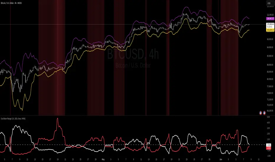
Euclidean Range [InvestorUnknown]The Euclidean Range indicator visualizes price deviation from a moving average using a geometric concept Euclidean distance. It helps traders identify trend strength, volatility shifts, and potential overextensions in price behavior.
Euclidean Distance
Euclidean distance is a fundamental concept in geometry and machine learning. It measures the "straight-line distance" between two points in space. In time series analysis, it can be used to measure how far one sequence deviates from another over a fixed window.
euclidean_distance(src, ref, len) =>
var float sum_sq_diff = na
sum_sq_diff := 0.0
for i = 0 to len - 1
diff = src - ref
sum_sq_diff += diff * diff
math.sqrt(sum_sq_diff)
In this script, we calculate the Euclidean distance between the price (source) and a smoothed average (reference) over a user-defined window. This gives us a single scalar that reflects the overall divergence between price and trend.
How It Works
Moving Average Calculation: You can choose between SMA, EMA, or HMA as your reference line. This becomes the "baseline" against which the actual price is compared.
Distance Band Construction: The Euclidean distance between the price and the reference is calculated over the Window Length. This value is then added to and subtracted from the average to form dynamic upper and lower bands, visually framing the range of deviation.
Distance Ratios and Z-Scores: Two distance ratios are computed: dist_r = distance / price (sensitivity to volatility); dist_v = price / distance (sensitivity to compression or low-volatility states)
Both ratios are normalized using a Z-score to standardize their behavior and allow for easier interpretation across different assets and timeframes.
Z-Score Plots: Z_r (white line) highlights instances of high volatility or strong price deviation; Z_v (red line) highlights low volatility or compressed price ranges.
Background Highlighting (Optional): When Z_v is dominant and increasing, the background is colored using a gradient. This signals a possible build-up in low volatility, which may precede a breakout.
Use Cases
Detect volatile expansions and calm compression zones.
Identify mean reversion setups when price returns to the average.
Anticipate breakout conditions by observing rising Z_v values.
Use dynamic distance bands as adaptive support/resistance zones.
Notes
The indicator is best used with liquid assets and medium-to-long windows.
Background coloring helps visually filter for squeeze setups.
Disclaimer
This indicator is provided for speculative analysis and educational purposes only. It is not financial advice. Always backtest and evaluate in a simulated environment before live trading.
DWMY Opens (for aggr. charts) by Koenigsegg🟣 DWMY Opens (for Aggregated Charts) by Koenigsegg
Revolutionary compatibility with aggregated charts – This indicator represents a significant breakthrough in displaying Daily, Weekly, Monthly, and Yearly opening levels on aggregated chart types where traditional DWMY indicators have historically failed to function properly.
Complete aggregated chart support – Unlike previous Daily Weekly Monthly Yearly Opens indicators that experienced severe limitations when pulling data from non-standard chart types, this version is specifically engineered to work flawlessly with aggregated charts, range bars, Renko charts, Point & Figure charts, and all other non-time-based chart constructions.
Persistent horizontal reference lines – The indicator draws four distinct horizontal lines representing the opening prices of the current Daily, Weekly, Monthly, and Yearly periods, extending these levels forward into future bars to provide clear reference points for key support and resistance analysis.
Advanced customization capabilities – Features comprehensive user controls including custom label naming for each timeframe, adjustable line colors with independent color selection for Daily, Weekly, Monthly, and Yearly levels, configurable line width settings, and variable label font sizes ranging from tiny to huge.
Dynamic label positioning system – Implements a sophisticated label placement mechanism with configurable tick offset positioning and fixed end-bars-ahead projection, ensuring labels remain visible and properly positioned regardless of chart zoom level or timeframe.
Intelligent period detection logic – Utilizes advanced Pine Script time change detection algorithms specifically optimized for aggregated charts, accurately identifying new Daily, Weekly, Monthly, and Yearly periods even when traditional time-based functions fail on non-standard chart types.
Performance-optimized architecture – Built with efficient persistent variable storage using the var keyword, minimizing computational overhead while maintaining real-time updates across all timeframe levels simultaneously.
Professional visual presentation – Delivers clean, uncluttered chart visualization with strategically positioned labels that clearly identify each timeframe level without interfering with price action analysis.
Universal market compatibility – Functions seamlessly across all asset classes including stocks, forex, cryptocurrencies, commodities, and indices, adapting automatically to different tick sizes and price scales through syminfo.mintick integration.
Pine Script v6 foundation – Leverages the latest Pine Script version 6 capabilities, ensuring optimal performance, stability, and compatibility with current and future TradingView platform updates.
This indicator solves a critical limitation that has long plagued traders using aggregated chart types, finally enabling reliable access to essential Daily, Weekly, Monthly, and Yearly opening levels that serve as fundamental support and resistance zones in technical analysis. The breakthrough lies in its ability to maintain accurate period detection and level plotting regardless of the underlying chart construction methodology.
🟣 How It Works
Automatic period detection – The indicator continuously monitors for time changes across four distinct timeframes using ta.change(time()) functions for Daily and Weekly periods, month transitions for Monthly levels, and year changes for Yearly opens, ensuring precise identification of new period beginnings.
Real-time level updates – When a new period is detected, the indicator captures the opening price at that exact moment and immediately establishes a horizontal line from that bar extending forward to a configurable number of bars ahead, creating persistent reference levels.
Dynamic line management – Each timeframe maintains its own dedicated line object and label, with the indicator continuously updating the endpoint coordinates and label positions as new bars form, ensuring the levels always project the specified distance into the future.
Intelligent label placement – Labels are positioned at the end of each line with automatic vertical offset based on the symbol’s minimum tick size, preventing overlap with price action while maintaining clear identification of each timeframe level.
🟣 Pro Tips for Optimal Usage
Multi-timeframe confluence – Look for areas where multiple DWMY levels converge within close proximity, as these zones typically act as stronger support or resistance levels due to increased market participant attention at these psychological price points.
Breakout confirmation strategy – When price breaks above or below a significant DWMY level with strong volume, the broken level often transforms into support (if broken upward) or resistance (if broken downward), providing excellent entry and exit reference points.
Range trading opportunities – On ranging markets, use Daily and Weekly opens as potential reversal zones, especially when price approaches these levels during low-volume periods or near session opens when institutional activity increases.
Timeframe alignment technique – For swing trading, prioritize trades that align with the direction of the break from Weekly or Monthly opens, while using Daily opens for precise entry timing and position management.
Chart type optimization – This indicator excels on Renko, Range, and Point & Figure charts where traditional time-based DWMY indicators fail, making it invaluable for traders who prefer these aggregated chart types for cleaner price action analysis.
Important Disclaimer:
This indicator is provided for educational and informational purposes only. It is not financial advice, investment advice, or a recommendation to buy or sell any financial instrument. All trading involves risk, and past performance does not guarantee future results. Please conduct your own research and consult with a qualified financial advisor before making any trading decisions. The author is not responsible for any losses incurred from using this indicator.

Bear Market Probability Model# Bear Market Probability Model: A Multi-Factor Risk Assessment Framework
The Bear Market Probability Model represents a comprehensive quantitative framework for assessing systemic market risk through the integration of 13 distinct risk factors across four analytical categories: macroeconomic indicators, technical analysis factors, market sentiment measures, and market breadth metrics. This indicator synthesizes established financial research methodologies to provide real-time probabilistic assessments of impending bear market conditions, offering institutional-grade risk management capabilities to retail and professional traders alike.
## Theoretical Foundation
### Historical Context of Bear Market Prediction
Bear market prediction has been a central focus of financial research since the seminal work of Dow (1901) and the subsequent development of technical analysis theory. The challenge of predicting market downturns gained renewed academic attention following the market crashes of 1929, 1987, 2000, and 2008, leading to the development of sophisticated multi-factor models.
Fama and French (1989) demonstrated that certain financial variables possess predictive power for stock returns, particularly during market stress periods. Their three-factor model laid the groundwork for multi-dimensional risk assessment, which this indicator extends through the incorporation of real-time market microstructure data.
### Methodological Framework
The model employs a weighted composite scoring methodology based on the theoretical framework established by Campbell and Shiller (1998) for market valuation assessment, extended through the incorporation of high-frequency sentiment and technical indicators as proposed by Baker and Wurgler (2006) in their seminal work on investor sentiment.
The mathematical foundation follows the general form:
Bear Market Probability = Σ(Wi × Ci) / ΣWi × 100
Where:
- Wi = Category weight (i = 1,2,3,4)
- Ci = Normalized category score
- Categories: Macroeconomic, Technical, Sentiment, Breadth
## Component Analysis
### 1. Macroeconomic Risk Factors
#### Yield Curve Analysis
The inclusion of yield curve inversion as a primary predictor follows extensive research by Estrella and Mishkin (1998), who demonstrated that the term spread between 3-month and 10-year Treasury securities has historically preceded all major recessions since 1969. The model incorporates both the 2Y-10Y and 3M-10Y spreads to capture different aspects of monetary policy expectations.
Implementation:
- 2Y-10Y Spread: Captures market expectations of monetary policy trajectory
- 3M-10Y Spread: Traditional recession predictor with 12-18 month lead time
Scientific Basis: Harvey (1988) and subsequent research by Ang, Piazzesi, and Wei (2006) established the theoretical foundation linking yield curve inversions to economic contractions through the expectations hypothesis of the term structure.
#### Credit Risk Premium Assessment
High-yield credit spreads serve as a real-time gauge of systemic risk, following the methodology established by Gilchrist and Zakrajšek (2012) in their excess bond premium research. The model incorporates the ICE BofA High Yield Master II Option-Adjusted Spread as a proxy for credit market stress.
Threshold Calibration:
- Normal conditions: < 350 basis points
- Elevated risk: 350-500 basis points
- Severe stress: > 500 basis points
#### Currency and Commodity Stress Indicators
The US Dollar Index (DXY) momentum serves as a risk-off indicator, while the Gold-to-Oil ratio captures commodity market stress dynamics. This approach follows the methodology of Akram (2009) and Beckmann, Berger, and Czudaj (2015) in analyzing commodity-currency relationships during market stress.
### 2. Technical Analysis Factors
#### Multi-Timeframe Moving Average Analysis
The technical component incorporates the well-established moving average convergence methodology, drawing from the work of Brock, Lakonishok, and LeBaron (1992), who provided empirical evidence for the profitability of technical trading rules.
Implementation:
- Price relative to 50-day and 200-day simple moving averages
- Moving average convergence/divergence analysis
- Multi-timeframe MACD assessment (daily and weekly)
#### Momentum and Volatility Analysis
The model integrates Relative Strength Index (RSI) analysis following Wilder's (1978) original methodology, combined with maximum drawdown analysis based on the work of Magdon-Ismail and Atiya (2004) on optimal drawdown measurement.
### 3. Market Sentiment Factors
#### Volatility Index Analysis
The VIX component follows the established research of Whaley (2009) and subsequent work by Bekaert and Hoerova (2014) on VIX as a predictor of market stress. The model incorporates both absolute VIX levels and relative VIX spikes compared to the 20-day moving average.
Calibration:
- Low volatility: VIX < 20
- Elevated concern: VIX 20-25
- High fear: VIX > 25
- Panic conditions: VIX > 30
#### Put-Call Ratio Analysis
Options flow analysis through put-call ratios provides insight into sophisticated investor positioning, following the methodology established by Pan and Poteshman (2006) in their analysis of informed trading in options markets.
### 4. Market Breadth Factors
#### Advance-Decline Analysis
Market breadth assessment follows the classic work of Fosback (1976) and subsequent research by Brown and Cliff (2004) on market breadth as a predictor of future returns.
Components:
- Daily advance-decline ratio
- Advance-decline line momentum
- McClellan Oscillator (Ema19 - Ema39 of A-D difference)
#### New Highs-New Lows Analysis
The new highs-new lows ratio serves as a market leadership indicator, based on the research of Zweig (1986) and validated in academic literature by Zarowin (1990).
## Dynamic Threshold Methodology
The model incorporates adaptive thresholds based on rolling volatility and trend analysis, following the methodology established by Pagan and Sossounov (2003) for business cycle dating. This approach allows the model to adjust sensitivity based on prevailing market conditions.
Dynamic Threshold Calculation:
- Warning Level: Base threshold ± (Volatility × 1.0)
- Danger Level: Base threshold ± (Volatility × 1.5)
- Bounds: ±10-20 points from base threshold
## Professional Implementation
### Institutional Usage Patterns
Professional risk managers typically employ multi-factor bear market models in several contexts:
#### 1. Portfolio Risk Management
- Tactical Asset Allocation: Reducing equity exposure when probability exceeds 60-70%
- Hedging Strategies: Implementing protective puts or VIX calls when warning thresholds are breached
- Sector Rotation: Shifting from growth to defensive sectors during elevated risk periods
#### 2. Risk Budgeting
- Value-at-Risk Adjustment: Incorporating bear market probability into VaR calculations
- Stress Testing: Using probability levels to calibrate stress test scenarios
- Capital Requirements: Adjusting regulatory capital based on systemic risk assessment
#### 3. Client Communication
- Risk Reporting: Quantifying market risk for client presentations
- Investment Committee Decisions: Providing objective risk metrics for strategic decisions
- Performance Attribution: Explaining defensive positioning during market stress
### Implementation Framework
Professional traders typically implement such models through:
#### Signal Hierarchy:
1. Probability < 30%: Normal risk positioning
2. Probability 30-50%: Increased hedging, reduced leverage
3. Probability 50-70%: Defensive positioning, cash building
4. Probability > 70%: Maximum defensive posture, short exposure consideration
#### Risk Management Integration:
- Position Sizing: Inverse relationship between probability and position size
- Stop-Loss Adjustment: Tighter stops during elevated risk periods
- Correlation Monitoring: Increased attention to cross-asset correlations
## Strengths and Advantages
### 1. Comprehensive Coverage
The model's primary strength lies in its multi-dimensional approach, avoiding the single-factor bias that has historically plagued market timing models. By incorporating macroeconomic, technical, sentiment, and breadth factors, the model provides robust risk assessment across different market regimes.
### 2. Dynamic Adaptability
The adaptive threshold mechanism allows the model to adjust sensitivity based on prevailing volatility conditions, reducing false signals during low-volatility periods and maintaining sensitivity during high-volatility regimes.
### 3. Real-Time Processing
Unlike traditional academic models that rely on monthly or quarterly data, this indicator processes daily market data, providing timely risk assessment for active portfolio management.
### 4. Transparency and Interpretability
The component-based structure allows users to understand which factors are driving risk assessment, enabling informed decision-making about model signals.
### 5. Historical Validation
Each component has been validated in academic literature, providing theoretical foundation for the model's predictive power.
## Limitations and Weaknesses
### 1. Data Dependencies
The model's effectiveness depends heavily on the availability and quality of real-time economic data. Federal Reserve Economic Data (FRED) updates may have lags that could impact model responsiveness during rapidly evolving market conditions.
### 2. Regime Change Sensitivity
Like most quantitative models, the indicator may struggle during unprecedented market conditions or structural regime changes where historical relationships break down (Taleb, 2007).
### 3. False Signal Risk
Multi-factor models inherently face the challenge of balancing sensitivity with specificity. The model may generate false positive signals during normal market volatility periods.
### 4. Currency and Geographic Bias
The model focuses primarily on US market indicators, potentially limiting its effectiveness for global portfolio management or non-USD denominated assets.
### 5. Correlation Breakdown
During extreme market stress, correlations between risk factors may increase dramatically, reducing the model's diversification benefits (Forbes and Rigobon, 2002).
## References
Akram, Q. F. (2009). Commodity prices, interest rates and the dollar. Energy Economics, 31(6), 838-851.
Ang, A., Piazzesi, M., & Wei, M. (2006). What does the yield curve tell us about GDP growth? Journal of Econometrics, 131(1-2), 359-403.
Baker, M., & Wurgler, J. (2006). Investor sentiment and the cross‐section of stock returns. The Journal of Finance, 61(4), 1645-1680.
Baker, S. R., Bloom, N., & Davis, S. J. (2016). Measuring economic policy uncertainty. The Quarterly Journal of Economics, 131(4), 1593-1636.
Barber, B. M., & Odean, T. (2001). Boys will be boys: Gender, overconfidence, and common stock investment. The Quarterly Journal of Economics, 116(1), 261-292.
Beckmann, J., Berger, T., & Czudaj, R. (2015). Does gold act as a hedge or a safe haven for stocks? A smooth transition approach. Economic Modelling, 48, 16-24.
Bekaert, G., & Hoerova, M. (2014). The VIX, the variance premium and stock market volatility. Journal of Econometrics, 183(2), 181-192.
Brock, W., Lakonishok, J., & LeBaron, B. (1992). Simple technical trading rules and the stochastic properties of stock returns. The Journal of Finance, 47(5), 1731-1764.
Brown, G. W., & Cliff, M. T. (2004). Investor sentiment and the near-term stock market. Journal of Empirical Finance, 11(1), 1-27.
Campbell, J. Y., & Shiller, R. J. (1998). Valuation ratios and the long-run stock market outlook. The Journal of Portfolio Management, 24(2), 11-26.
Dow, C. H. (1901). Scientific stock speculation. The Magazine of Wall Street.
Estrella, A., & Mishkin, F. S. (1998). Predicting US recessions: Financial variables as leading indicators. Review of Economics and Statistics, 80(1), 45-61.
Fama, E. F., & French, K. R. (1989). Business conditions and expected returns on stocks and bonds. Journal of Financial Economics, 25(1), 23-49.
Forbes, K. J., & Rigobon, R. (2002). No contagion, only interdependence: measuring stock market comovements. The Journal of Finance, 57(5), 2223-2261.
Fosback, N. G. (1976). Stock market logic: A sophisticated approach to profits on Wall Street. The Institute for Econometric Research.
Gilchrist, S., & Zakrajšek, E. (2012). Credit spreads and business cycle fluctuations. American Economic Review, 102(4), 1692-1720.
Harvey, C. R. (1988). The real term structure and consumption growth. Journal of Financial Economics, 22(2), 305-333.
Kahneman, D., & Tversky, A. (1979). Prospect theory: An analysis of decision under risk. Econometrica, 47(2), 263-291.
Magdon-Ismail, M., & Atiya, A. F. (2004). Maximum drawdown. Risk, 17(10), 99-102.
Nickerson, R. S. (1998). Confirmation bias: A ubiquitous phenomenon in many guises. Review of General Psychology, 2(2), 175-220.
Pagan, A. R., & Sossounov, K. A. (2003). A simple framework for analysing bull and bear markets. Journal of Applied Econometrics, 18(1), 23-46.
Pan, J., & Poteshman, A. M. (2006). The information in option volume for future stock prices. The Review of Financial Studies, 19(3), 871-908.
Taleb, N. N. (2007). The black swan: The impact of the highly improbable. Random House.
Whaley, R. E. (2009). Understanding the VIX. The Journal of Portfolio Management, 35(3), 98-105.
Wilder, J. W. (1978). New concepts in technical trading systems. Trend Research.
Zarowin, P. (1990). Size, seasonality, and stock market overreaction. Journal of Financial and Quantitative Analysis, 25(1), 113-125.
Zweig, M. E. (1986). Winning on Wall Street. Warner Books.

pymath█ OVERVIEW
This library ➕ enhances Pine Script's built-in types (`float`, `int`, `array`, `array`) with mathematical methods, mirroring 🪞 many functions from Python's `math` module. Import this library to overload or add to built-in capabilities, enabling calls like `myFloat.sin()` or `myIntArray.gcd()`.
█ CONCEPTS
This library wraps Pine's built-in `math.*` functions and implements others where necessary, expanding the mathematical toolkit available within Pine Script. It provides a more object-oriented approach to mathematical operations on core data types.
█ HOW TO USE
• Import the library: i mport kaigouthro/pymath/1
• Call methods directly on variables: myFloat.sin() , myIntArray.gcd()
• For raw integer literals, you MUST use parentheses: `(1234).factorial()`.
█ FEATURES
• **Infinity Handling:** Includes `isinf()` and `isfinite()` for robust checks. Uses `POS_INF_PROXY` to represent infinity.
• **Comprehensive Math Functions:** Implements a wide range of methods, including trigonometric, logarithmic, hyperbolic, and array operations.
• **Object-Oriented Approach:** Allows direct method calls on `int`, `float`, and arrays for cleaner code.
• **Improved Accuracy:** Some functions (e.g., `remainder()`) offer improved accuracy compared to default Pine behavior.
• **Helper Functions:** Internal helper functions optimize calculations and handle edge cases.
█ NOTES
This library improves upon Pine Script's built-in `math` functions by adding new ones and refining existing implementations. It handles edge cases such as infinity, NaN, and zero values, enhancing the reliability of your Pine scripts. For Speed, it wraps and uses built-ins, as thy are fastest.
█ EXAMPLES
//@version=6
indicator("My Indicator")
// Import the library
import kaigouthro/pymath/1
// Create some Vars
float myFloat = 3.14159
int myInt = 10
array myIntArray = array.from(1, 2, 3, 4, 5)
// Now you can...
plot( myFloat.sin() ) // Use sin() method on a float, using built in wrapper
plot( (myInt).factorial() ) // Factorial of an integer (note parentheses)
plot( myIntArray.gcd() ) // GCD of an integer array
method isinf(self)
isinf: Checks if this float is positive or negative infinity using a proxy value.
Namespace types: series float, simple float, input float, const float
Parameters:
self (float) : (float) value to check.
Returns: (bool) `true` if the absolute value of `self` is greater than or equal to the infinity proxy, `false` otherwise.
method isfinite(self)
isfinite: Checks if this float is finite (not NaN and not infinity).
Namespace types: series float, simple float, input float, const float
Parameters:
self (float) : (float) The value to check.
Returns: (bool) `true` if `self` is not `na` and not infinity (as defined by `isinf()`), `false` otherwise.
method fmod(self, divisor)
fmod: Returns the C-library style floating-point remainder of `self / divisor` (result has the sign of `self`).
Namespace types: series float, simple float, input float, const float
Parameters:
self (float) : (float) Dividend `x`.
divisor (float) : (float) Divisor `y`. Cannot be zero or `na`.
Returns: (float) The remainder `x - n*y` where n is `trunc(x/y)`, or `na` if divisor is 0, `na`, or inputs are infinite in a way that prevents calculation.
method factorial(self)
factorial: Calculates the factorial of this non-negative integer.
Namespace types: series int, simple int, input int, const int
Parameters:
self (int) : (int) The integer `n`. Must be non-negative.
Returns: (float) `n!` as a float, or `na` if `n` is negative or overflow occurs (based on `isinf`).
method isqrt(self)
isqrt: Calculates the integer square root of this non-negative integer (floor of the exact square root).
Namespace types: series int, simple int, input int, const int
Parameters:
self (int) : (int) The non-negative integer `n`.
Returns: (int) The greatest integer `a` such that a² <= n, or `na` if `n` is negative.
method comb(self, k)
comb: Calculates the number of ways to choose `k` items from `self` items without repetition and without order (Binomial Coefficient).
Namespace types: series int, simple int, input int, const int
Parameters:
self (int) : (int) Total number of items `n`. Must be non-negative.
k (int) : (int) Number of items to choose. Must be non-negative.
Returns: (float) The binomial coefficient nCk, or `na` if inputs are invalid (n<0 or k<0), `k > n`, or overflow occurs.
method perm(self, k)
perm: Calculates the number of ways to choose `k` items from `self` items without repetition and with order (Permutations).
Namespace types: series int, simple int, input int, const int
Parameters:
self (int) : (int) Total number of items `n`. Must be non-negative.
k (simple int) : (simple int = na) Number of items to choose. Must be non-negative. Defaults to `n` if `na`.
Returns: (float) The number of permutations nPk, or `na` if inputs are invalid (n<0 or k<0), `k > n`, or overflow occurs.
method log2(self)
log2: Returns the base-2 logarithm of this float. Input must be positive. Wraps `math.log(self) / math.log(2.0)`.
Namespace types: series float, simple float, input float, const float
Parameters:
self (float) : (float) The input number. Must be positive.
Returns: (float) The base-2 logarithm, or `na` if input <= 0.
method trunc(self)
trunc: Returns this float with the fractional part removed (truncates towards zero).
Namespace types: series float, simple float, input float, const float
Parameters:
self (float) : (float) The input number.
Returns: (int) The integer part, or `na` if input is `na` or infinite.
method abs(self)
abs: Returns the absolute value of this float. Wraps `math.abs()`.
Namespace types: series float, simple float, input float, const float
Parameters:
self (float) : (float) The input number.
Returns: (float) The absolute value, or `na` if input is `na`.
method acos(self)
acos: Returns the arccosine of this float, in radians. Wraps `math.acos()`. Input must be between -1 and 1.
Namespace types: series float, simple float, input float, const float
Parameters:
self (float) : (float) The input number. Must be between -1 and 1.
Returns: (float) Angle in radians , or `na` if input is outside or `na`.
method asin(self)
asin: Returns the arcsine of this float, in radians. Wraps `math.asin()`. Input must be between -1 and 1.
Namespace types: series float, simple float, input float, const float
Parameters:
self (float) : (float) The input number. Must be between -1 and 1.
Returns: (float) Angle in radians , or `na` if input is outside or `na`.
method atan(self)
atan: Returns the arctangent of this float, in radians. Wraps `math.atan()`.
Namespace types: series float, simple float, input float, const float
Parameters:
self (float) : (float) The input number.
Returns: (float) Angle in radians , or `na` if input is `na`.
method ceil(self)
ceil: Returns the ceiling of this float (smallest integer >= self). Wraps `math.ceil()`.
Namespace types: series float, simple float, input float, const float
Parameters:
self (float) : (float) The input number.
Returns: (int) The ceiling value, or `na` if input is `na` or infinite.
method cos(self)
cos: Returns the cosine of this float (angle in radians). Wraps `math.cos()`.
Namespace types: series float, simple float, input float, const float
Parameters:
self (float) : (float) The angle in radians.
Returns: (float) The cosine, or `na` if input is `na`.
method degrees(self)
degrees: Converts this float from radians to degrees. Wraps `math.todegrees()`.
Namespace types: series float, simple float, input float, const float
Parameters:
self (float) : (float) The angle in radians.
Returns: (float) The angle in degrees, or `na` if input is `na`.
method exp(self)
exp: Returns e raised to the power of this float. Wraps `math.exp()`.
Namespace types: series float, simple float, input float, const float
Parameters:
self (float) : (float) The exponent.
Returns: (float) `e**self`, or `na` if input is `na`.
method floor(self)
floor: Returns the floor of this float (largest integer <= self). Wraps `math.floor()`.
Namespace types: series float, simple float, input float, const float
Parameters:
self (float) : (float) The input number.
Returns: (int) The floor value, or `na` if input is `na` or infinite.
method log(self)
log: Returns the natural logarithm (base e) of this float. Wraps `math.log()`. Input must be positive.
Namespace types: series float, simple float, input float, const float
Parameters:
self (float) : (float) The input number. Must be positive.
Returns: (float) The natural logarithm, or `na` if input <= 0 or `na`.
method log10(self)
log10: Returns the base-10 logarithm of this float. Wraps `math.log10()`. Input must be positive.
Namespace types: series float, simple float, input float, const float
Parameters:
self (float) : (float) The input number. Must be positive.
Returns: (float) The base-10 logarithm, or `na` if input <= 0 or `na`.
method pow(self, exponent)
pow: Returns this float raised to the power of `exponent`. Wraps `math.pow()`.
Namespace types: series float, simple float, input float, const float
Parameters:
self (float) : (float) The base.
exponent (float) : (float) The exponent.
Returns: (float) `self**exponent`, or `na` if inputs are `na` or lead to undefined results.
method radians(self)
radians: Converts this float from degrees to radians. Wraps `math.toradians()`.
Namespace types: series float, simple float, input float, const float
Parameters:
self (float) : (float) The angle in degrees.
Returns: (float) The angle in radians, or `na` if input is `na`.
method round(self)
round: Returns the nearest integer to this float. Wraps `math.round()`. Ties are rounded away from zero.
Namespace types: series float, simple float, input float, const float
Parameters:
self (float) : (float) The input number.
Returns: (int) The rounded integer, or `na` if input is `na` or infinite.
method sign(self)
sign: Returns the sign of this float (-1, 0, or 1). Wraps `math.sign()`.
Namespace types: series float, simple float, input float, const float
Parameters:
self (float) : (float) The input number.
Returns: (int) -1 if negative, 0 if zero, 1 if positive, `na` if input is `na`.
method sin(self)
sin: Returns the sine of this float (angle in radians). Wraps `math.sin()`.
Namespace types: series float, simple float, input float, const float
Parameters:
self (float) : (float) The angle in radians.
Returns: (float) The sine, or `na` if input is `na`.
method sqrt(self)
sqrt: Returns the square root of this float. Wraps `math.sqrt()`. Input must be non-negative.
Namespace types: series float, simple float, input float, const float
Parameters:
self (float) : (float) The input number. Must be non-negative.
Returns: (float) The square root, or `na` if input < 0 or `na`.
method tan(self)
tan: Returns the tangent of this float (angle in radians). Wraps `math.tan()`.
Namespace types: series float, simple float, input float, const float
Parameters:
self (float) : (float) The angle in radians.
Returns: (float) The tangent, or `na` if input is `na`.
method acosh(self)
acosh: Returns the inverse hyperbolic cosine of this float. Input must be >= 1.
Namespace types: series float, simple float, input float, const float
Parameters:
self (float) : (float) The input number. Must be >= 1.
Returns: (float) The inverse hyperbolic cosine, or `na` if input < 1 or `na`.
method asinh(self)
asinh: Returns the inverse hyperbolic sine of this float.
Namespace types: series float, simple float, input float, const float
Parameters:
self (float) : (float) The input number.
Returns: (float) The inverse hyperbolic sine, or `na` if input is `na`.
method atanh(self)
atanh: Returns the inverse hyperbolic tangent of this float. Input must be between -1 and 1 (exclusive).
Namespace types: series float, simple float, input float, const float
Parameters:
self (float) : (float) The input number. Must be between -1 and 1 (exclusive).
Returns: (float) The inverse hyperbolic tangent, or `na` if input is outside (-1, 1) or `na`.
method cosh(self)
cosh: Returns the hyperbolic cosine of this float.
Namespace types: series float, simple float, input float, const float
Parameters:
self (float) : (float) The input number.
Returns: (float) The hyperbolic cosine, or `na` if input is `na`.
method sinh(self)
sinh: Returns the hyperbolic sine of this float.
Namespace types: series float, simple float, input float, const float
Parameters:
self (float) : (float) The input number.
Returns: (float) The hyperbolic sine, or `na` if input is `na`.
method tanh(self)
tanh: Returns the hyperbolic tangent of this float.
Namespace types: series float, simple float, input float, const float
Parameters:
self (float) : (float) The input number.
Returns: (float) The hyperbolic tangent, or `na` if input is `na`.
method atan2(self, dx)
atan2: Returns the angle in radians between the positive x-axis and the point (dx, self). Wraps `math.atan2()`.
Namespace types: series float, simple float, input float, const float
Parameters:
self (float) : (float) The y-coordinate `y`.
dx (float) : (float) The x-coordinate `x`.
Returns: (float) The angle in radians , result of `math.atan2(self, dx)`. Returns `na` if inputs are `na`. Note: `math.atan2(0, 0)` returns 0 in Pine.
Optimization: Use built-in math.atan2()
method cbrt(self)
cbrt: Returns the cube root of this float.
Namespace types: series float, simple float, input float, const float
Parameters:
self (float) : (float) The value to find the cube root of.
Returns: (float) The real cube root. Handles negative inputs correctly, or `na` if input is `na`.
method exp2(self)
exp2: Returns 2 raised to the power of this float. Calculated as `2.0.pow(self)`.
Namespace types: series float, simple float, input float, const float
Parameters:
self (float) : (float) The exponent.
Returns: (float) `2**self`, or `na` if input is `na` or results in non-finite value.
method expm1(self)
expm1: Returns `e**self - 1`. Calculated as `self.exp() - 1.0`. May offer better precision for small `self` in some environments, but Pine provides no guarantee over `self.exp() - 1.0`.
Namespace types: series float, simple float, input float, const float
Parameters:
self (float) : (float) The exponent.
Returns: (float) `e**self - 1`, or `na` if input is `na` or `self.exp()` is `na`.
method log1p(self)
log1p: Returns the natural logarithm of (1 + self). Calculated as `(1.0 + self).log()`. Pine provides no specific precision guarantee for self near zero.
Namespace types: series float, simple float, input float, const float
Parameters:
self (float) : (float) Value to add to 1. `1 + self` must be positive.
Returns: (float) Natural log of `1 + self`, or `na` if input is `na` or `1 + self <= 0`.
method modf(self)
modf: Returns the fractional and integer parts of this float as a tuple ` `. Both parts have the sign of `self`.
Namespace types: series float, simple float, input float, const float
Parameters:
self (float) : (float) The number `x` to split.
Returns: ( ) A tuple containing ` `, or ` ` if `x` is `na` or non-finite.
method remainder(self, divisor)
remainder: Returns the IEEE 754 style remainder of `self` with respect to `divisor`. Result `r` satisfies `abs(r) <= 0.5 * abs(divisor)`. Uses round-half-to-even.
Namespace types: series float, simple float, input float, const float
Parameters:
self (float) : (float) Dividend `x`.
divisor (float) : (float) Divisor `y`. Cannot be zero or `na`.
Returns: (float) The IEEE 754 remainder, or `na` if divisor is 0, `na`, or inputs are non-finite in a way that prevents calculation.
method copysign(self, signSource)
copysign: Returns a float with the magnitude (absolute value) of `self` but the sign of `signSource`.
Namespace types: series float, simple float, input float, const float
Parameters:
self (float) : (float) Value providing the magnitude `x`.
signSource (float) : (float) Value providing the sign `y`.
Returns: (float) `abs(x)` with the sign of `y`, or `na` if either input is `na`.
method frexp(self)
frexp: Returns the mantissa (m) and exponent (e) of this float `x` as ` `, such that `x = m * 2^e` and `0.5 <= abs(m) < 1` (unless `x` is 0).
Namespace types: series float, simple float, input float, const float
Parameters:
self (float) : (float) The number `x` to decompose.
Returns: ( ) A tuple ` `, or ` ` if `x` is 0, or ` ` if `x` is non-finite or `na`.
method isclose(self, other, rel_tol, abs_tol)
isclose: Checks if this float `a` and `other` float `b` are close within relative and absolute tolerances.
Namespace types: series float, simple float, input float, const float
Parameters:
self (float) : (float) First value `a`.
other (float) : (float) Second value `b`.
rel_tol (simple float) : (simple float = 1e-9) Relative tolerance. Must be non-negative and less than 1.0.
abs_tol (simple float) : (simple float = 0.0) Absolute tolerance. Must be non-negative.
Returns: (bool) `true` if `abs(a - b) <= max(rel_tol * max(abs(a), abs(b)), abs_tol)`. Handles `na`/`inf` appropriately. Returns `na` if tolerances are invalid.
method ldexp(self, exponent)
ldexp: Returns `self * (2**exponent)`. Inverse of `frexp`.
Namespace types: series float, simple float, input float, const float
Parameters:
self (float) : (float) Mantissa part `x`.
exponent (int) : (int) Exponent part `i`.
Returns: (float) The result of `x * pow(2, i)`, or `na` if inputs are `na` or result is non-finite.
method gcd(self)
gcd: Calculates the Greatest Common Divisor (GCD) of all integers in this array.
Namespace types: array
Parameters:
self (array) : (array) An array of integers.
Returns: (int) The largest positive integer that divides all non-zero elements, 0 if all elements are 0 or array is empty. Returns `na` if any element is `na`.
method lcm(self)
lcm: Calculates the Least Common Multiple (LCM) of all integers in this array.
Namespace types: array
Parameters:
self (array) : (array) An array of integers.
Returns: (int) The smallest positive integer that is a multiple of all non-zero elements, 0 if any element is 0, 1 if array is empty. Returns `na` on potential overflow or if any element is `na`.
method dist(self, other)
dist: Returns the Euclidean distance between this point `p` and another point `q` (given as arrays of coordinates).
Namespace types: array
Parameters:
self (array) : (array) Coordinates of the first point `p`.
other (array) : (array) Coordinates of the second point `q`. Must have the same size as `p`.
Returns: (float) The Euclidean distance, or `na` if arrays have different sizes, are empty, or contain `na`/non-finite values.
method fsum(self)
fsum: Returns an accurate floating-point sum of values in this array. Uses built-in `array.sum()`. Note: Pine Script does not guarantee the same level of precision tracking as Python's `math.fsum`.
Namespace types: array
Parameters:
self (array) : (array) The array of floats to sum.
Returns: (float) The sum of the array elements. Returns 0.0 for an empty array. Returns `na` if any element is `na`.
method hypot(self)
hypot: Returns the Euclidean norm (distance from origin) for this point given by coordinates in the array. `sqrt(sum(x*x for x in coordinates))`.
Namespace types: array
Parameters:
self (array) : (array) Array of coordinates defining the point.
Returns: (float) The Euclidean norm, or 0.0 if the array is empty. Returns `na` if any element is `na` or non-finite.
method prod(self, start)
prod: Calculates the product of all elements in this array.
Namespace types: array
Parameters:
self (array) : (array) The array of values to multiply.
start (simple float) : (simple float = 1.0) The starting value for the product (returned if the array is empty).
Returns: (float) The product of array elements * start. Returns `na` if any element is `na`.
method sumprod(self, other)
sumprod: Returns the sum of products of values from this array `p` and another array `q` (dot product).
Namespace types: array
Parameters:
self (array) : (array) First array of values `p`.
other (array) : (array) Second array of values `q`. Must have the same size as `p`.
Returns: (float) The sum of `p * q ` for all i, or `na` if arrays have different sizes or contain `na`/non-finite values. Returns 0.0 for empty arrays.

ICT Order Blocks v2 (Debug)Josh has a very large PP xD
Understanding Order Blocks (OBs) - The ICT Perspective
This document delves into the concept of Order Blocks (OBs) from the perspective of the ICT methodology. It outlines what OBs are, their significance in trading, and how the "ICT Order Blocks v2 (Refined)" indicator functions to identify and visualize these critical price levels. By understanding OBs, traders can better navigate market movements and make informed decisions based on institutional trading behavior.
What is an Order Block (OB)?
Within ICT methodology, an Order Block represents a specific price candle where significant buying or selling interest from institutions (Smart Money) is believed to have occurred. They are potential areas where price might return and react.
Bullish Order Block: Typically the last down-closing candle before a strong, impulsive upward move (displacement). It suggests institutions may have absorbed selling pressure and initiated long positions here.
Bearish Order Block: Typically the last up-closing candle before a strong, impulsive downward move (displacement). It suggests institutions may have distributed long positions or initiated short positions here.
Why are OBs Significant (ICT View)?
Institutional Footprint: They mark potential zones of large order execution.
Support/Resistance: Unmitigated OBs can act as sensitive price levels where reactions are expected. Bullish OBs may provide support; Bearish OBs may provide resistance.
Origin of Moves: They often mark the origin point of significant price swings.
Liquidity Engineering: Institutions might drive price back to OBs to mitigate earlier positions or to engineer liquidity before continuing a move.
Common Refinements
ICT often emphasizes higher probability OBs that are associated with:
Displacement: The move away from the OB is sharp and decisive.
Fair Value Gaps (FVGs): An FVG forming immediately after the OB strengthens its validity.
OB Mitigation: This refers to price returning to the level of the Order Block after its formation. Price might react at the edge (proximal line) or the 50% level (mean threshold) of the OB. An OB is often considered fully mitigated or invalidated if price trades decisively through its entire range, especially with a candle body closing beyond it.
How the "ICT Order Blocks v2 (Refined)" Indicator Works
This indicator automates the detection and visualization of the most recent unmitigated Order Block of each type (Bullish/Bearish), incorporating optional filters.
Detection:
It looks at the relationship between the candle two bars ago ( ), the previous candle ( ), and potentially the current candle ( ).
Bullish OB: Identifies if candle was a down-close (close < open ) AND candle broke above the high of candle (high > high ).
Bearish OB: Identifies if candle was an up-close (close > open ) AND candle broke below the low of candle (low < low ).
Accuracy Filters (Optional Inputs):
These filters help identify potentially higher-probability OBs:
Require Fair Value Gap (FVG)?: If enabled, the indicator checks if an FVG formed immediately after the OB candle ( ). Specifically, it looks for a gap between candle and candle (low > high for Bullish OB confirmation, high < low for Bearish).
Require Strong Close Breakout?: If enabled, it requires the breakout candle ( ) to close beyond the range of the OB candle ( ). (close > high for Bullish, close < low for Bearish). This suggests stronger confirmation.
Storing the Most Recent OB:
When an OB is detected and passes any enabled filters, its details (high, low, formation bar index) are stored. Crucially, this indicator only tracks the single most recent valid unmitigated OB of each type (one Bullish, one Bearish) using var variables. If a newer valid OB forms, it replaces the previously stored one.
Drawing Boxes:
If a valid Bullish OB is being tracked (and Show Bullish OBs is enabled), it draws a box (box.new) using the high and low of the identified OB candle ( ). The same process applies to Bearish OBs (Show Bearish OBs enabled). The boxes automatically extend to the right (extend.right) and their right edge is updated on each new bar (box.set_right) until they are mitigated. Labels ("Bull OB" / "Bear OB") are displayed inside the boxes.
Mitigation & Box Deletion:
The indicator checks if the current closing price (close ) has moved entirely beyond the range of the tracked OB.
Mitigation Rule Used: A Bullish OB is considered mitigated if close < bull_ob_low. A Bearish OB is considered mitigated if close > bear_ob_high. Once an OB is marked as mitigated, the indicator stops tracking it and its corresponding box is automatically deleted (box.delete) from the chart.
This indicator provides a dynamic visualization of the most recent, potentially significant Order Blocks that meet the specified criteria, helping traders identify key areas of interest based on ICT principles.
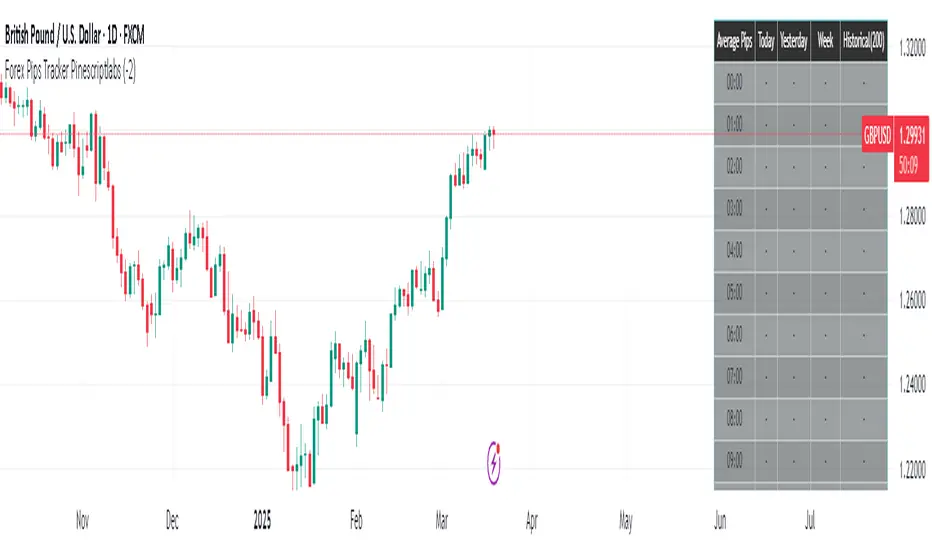
Forex Pips Tracker PinescriptlabsThis algorithm is exclusively designed for the Forex market 🌐 and serves as a tool to measure volatility, helping to determine on average how many pips positions move per hour. With this information, a trader can place take profit and stop loss orders with greater certainty, since they know the average pip movement range during each hour of the day.
What does it do and how does it work?
• Volatility measurement in pips 📊:
The algorithm calculates the size of the movement (or range) of each candle expressed in pips. To do this, it takes the difference between the highest and lowest price of each candle and converts it into pips.
👉
• Time zone adjustment ⏰:
It allows you to configure the time zone so that the data aligns with your desired schedule. This is especially useful for comparing movements at different times based on the trader's location.
• Analysis by time intervals 🕒:
The algorithm’s logic organizes the information for each hour of the day. It stores data for the current day, the previous day, weekly, and historically (200 candles). This allows you to see how volatility varies across different periods, providing a dynamic view of market behavior.
👉
• Directionality of movement 🔄:
In addition to averaging the pip range, the algorithm determines the predominant direction of each candle (bullish or bearish). This translates into visual indicators (like arrows) that help identify whether, on average, the movement during that hour tends to go up or down.
• Table visualization 📈:
Finally, the information is presented in an integrated table on the chart. Each row corresponds to an hour of the day and shows the average number of pips and the direction (bullish, bearish, or neutral) for each analyzed period. This table makes it easy to quickly and practically interpret the volatility data.
By combining these features, the algorithm becomes an essential tool for traders looking to better understand market dynamics and optimize their trading strategies! 💼✨
Español:
Este algoritmo está diseñado exclusivamente para el mercado Forex 🌐 y sirve como una herramienta para medir la volatilidad, ayudando a determinar en promedio cuántos pips se mueven las posiciones por hora. Con esta información, un trader puede colocar el take profit y el stop loss con mayor certeza, ya que conoce el rango promedio de movimiento en pips durante cada hora del día.
¿Qué hace y cómo funciona?
• Medición de volatilidad en pips 📊:
El algoritmo calcula el tamaño del movimiento (o rango) de cada vela expresado en pips. Para ello, toma la diferencia entre el precio máximo y el mínimo de cada vela y la convierte a pips.
👉
• Ajuste de zona horaria ⏰:
Permite configurar la zona horaria para que los datos se ajusten al horario deseado. Esto es especialmente útil para comparar movimientos durante distintas horas en función de la localización del trader.
• Análisis por intervalos de tiempo 🕒:
La lógica del algoritmo organiza la información por cada hora del día. Guarda datos para el día actual, el día anterior, a nivel semanal e histórico (200 velas). Esto permite ver cómo varía la volatilidad en diferentes periodos, proporcionando una visión dinámica del comportamiento del mercado.
👉
• Direccionalidad del movimiento 🔄:
Además de promediar el rango en pips, el algoritmo determina la dirección predominante de cada vela (alcista o bajista). Esto se traduce en indicadores visuales (como flechas) que permiten identificar si, en promedio, el movimiento en esa hora tiende a subir o bajar.
• Visualización en tabla 📈:
Finalmente, la información se presenta en una tabla integrada en el gráfico. Cada fila corresponde a una hora del día y muestra el promedio de pips y la dirección (alcista, bajista o neutral) para cada uno de los periodos analizados. Esta tabla facilita la interpretación rápida y práctica de los datos de volatilidad.
Al combinar estas funciones, el algoritmo se convierte en una herramienta esencial para traders que buscan entender mejor la dinámica del mercado y optimizar sus estrategias de trading! 💼✨
iD EMARSI on ChartSCRIPT OVERVIEW
The EMARSI indicator is an advanced technical analysis tool that maps RSI values directly onto price charts. With adaptive scaling capabilities, it provides a unique visualization of momentum that flows naturally with price action, making it particularly valuable for FOREX and low-priced securities trading.
KEY FEATURES
1 PRICE MAPPED RSI VISUALIZATION
Unlike traditional RSI that displays in a separate window, EMARSI plots the RSI directly on the price chart, creating a flowing line that identifies momentum shifts within the context of price action:
// Map RSI to price chart with better scaling
mappedRsi = useAdaptiveScaling ?
median + ((rsi - 50) / 50 * (pQH - pQL) / 2 * math.min(1.0, 1/scalingFactor)) :
down == pQL ? pQH : up == pQL ? pQL : median - (median / (1 + up / down))
2 ADAPTIVE SCALING SYSTEM
The script features an intelligent scaling system that automatically adjusts to different market conditions and price levels:
// Calculate adaptive scaling factor based on selected method
scalingFactor = if scalingMethod == "ATR-Based"
math.min(maxScalingFactor, math.max(1.0, minTickSize / (atrValue/avgPrice)))
else if scalingMethod == "Price-Based"
math.min(maxScalingFactor, math.max(1.0, math.sqrt(100 / math.max(avgPrice, 0.01))))
else // Volume-Based
math.min(maxScalingFactor, math.max(1.0, math.sqrt(1000000 / math.max(volume, 100))))
3 MODIFIED RSI CALCULATION
EMARSI uses a specially formulated RSI calculation that works with an adaptive base value to maintain consistency across different price ranges:
// Adaptive RSI Base based on price levels to improve flow
adaptiveRsiBase = useAdaptiveScaling ? rsiBase * scalingFactor : rsiBase
// Calculate RSI components with adaptivity
up = ta.rma(math.max(ta.change(rsiSourceInput), adaptiveRsiBase), emaSlowLength)
down = ta.rma(-math.min(ta.change(rsiSourceInput), adaptiveRsiBase), rsiLengthInput)
// Improved RSI calculation with value constraint
rsi = down == 0 ? 100 : up == 0 ? 0 : 100 - (100 / (1 + up / down))
4 MOVING AVERAGE CROSSOVER SYSTEM
The indicator creates a smooth moving average of the RSI line, enabling a crossover system that generates trading signals:
// Calculate MA of mapped RSI
rsiMA = ma(mappedRsi, emaSlowLength, maTypeInput)
// Strategy entries
if ta.crossover(mappedRsi, rsiMA)
strategy.entry("RSI Long", strategy.long)
if ta.crossunder(mappedRsi, rsiMA)
strategy.entry("RSI Short", strategy.short)
5 VISUAL REFERENCE FRAMEWORK
The script includes visual guides that help interpret the RSI movement within the context of recent price action:
// Calculate pivot high and low
pQH = ta.highest(high, hlLen)
pQL = ta.lowest(low, hlLen)
median = (pQH + pQL) / 2
// Plotting
plot(pQH, "Pivot High", color=color.rgb(82, 228, 102, 90))
plot(pQL, "Pivot Low", color=color.rgb(231, 65, 65, 90))
med = plot(median, style=plot.style_steplinebr, linewidth=1, color=color.rgb(238, 101, 59, 90))
6 DYNAMIC COLOR SYSTEM
The indicator uses color fills to clearly visualize the relationship between the RSI and its moving average:
// Color fills based on RSI vs MA
colUp = mappedRsi > rsiMA ? input.color(color.rgb(128, 255, 0), '', group= 'RSI > EMA', inline= 'up') :
input.color(color.rgb(240, 9, 9, 95), '', group= 'RSI < EMA', inline= 'dn')
colDn = mappedRsi > rsiMA ? input.color(color.rgb(0, 230, 35, 95), '', group= 'RSI > EMA', inline= 'up') :
input.color(color.rgb(255, 47, 0), '', group= 'RSI < EMA', inline= 'dn')
fill(rsiPlot, emarsi, mappedRsi > rsiMA ? pQH : rsiMA, mappedRsi > rsiMA ? rsiMA : pQL, colUp, colDn)
7 REAL TIME PARAMETER MONITORING
A transparent information panel provides real-time feedback on the adaptive parameters being applied:
// Information display
var table infoPanel = table.new(position.top_right, 2, 3, bgcolor=color.rgb(0, 0, 0, 80))
if barstate.islast
table.cell(infoPanel, 0, 0, "Current Scaling Factor", text_color=color.white)
table.cell(infoPanel, 1, 0, str.tostring(scalingFactor, "#.###"), text_color=color.white)
table.cell(infoPanel, 0, 1, "Adaptive RSI Base", text_color=color.white)
table.cell(infoPanel, 1, 1, str.tostring(adaptiveRsiBase, "#.####"), text_color=color.white)
BENEFITS FOR TRADERS
INTUITIVE MOMENTUM VISUALIZATION
By mapping RSI directly onto the price chart, traders can immediately see the relationship between momentum and price without switching between different indicator windows.
ADAPTIVE TO ANY MARKET CONDITION
The three scaling methods (ATR-Based, Price-Based, and Volume-Based) ensure the indicator performs consistently across different market conditions, volatility regimes, and price levels.
PREVENTS EXTREME VALUES
The adaptive scaling system prevents the RSI from generating extreme values that exceed chart boundaries when trading low-priced securities or during high volatility periods.
CLEAR TRADING SIGNALS
The RSI and moving average crossover system provides clear entry signals that are visually reinforced through color changes, making it easy to identify potential trading opportunities.
SUITABLE FOR MULTIPLE TIMEFRAMES
The indicator works effectively across multiple timeframes, from intraday to daily charts, making it versatile for different trading styles and strategies.
TRANSPARENT PARAMETER ADJUSTMENT
The information panel provides real-time feedback on how the adaptive system is adjusting to current market conditions, helping traders understand why the indicator is behaving as it is.
CUSTOMIZABLE VISUALIZATION
Multiple visualization options including Bollinger Bands, different moving average types, and customizable colors allow traders to adapt the indicator to their personal preferences.
CONCLUSION
The EMARSI indicator represents a significant advancement in RSI visualization by directly mapping momentum onto price charts with adaptive scaling. This approach makes momentum shifts more intuitive to identify and helps prevent the scaling issues that commonly affect RSI-based indicators when applied to low-priced securities or volatile markets.
Shadow Edge (Example)This script tracks hourly price extremes (highs/lows) and their equilibrium (midpoint), plotting them as dynamic reference lines on your chart. It helps visualize intraday support/resistance levels and potential price boundaries.
Key Features
Previous Hour Levels (Static Lines):
PH (Previous Hour High): Red line.
PL (Previous Hour Low): Green line.
P.EQ (Previous Hour Equilibrium): Blue midpoint between PH and PL.
Current Hour Levels (Dynamic/Dotted Lines):
MuEH (Current Hour High): Yellow dashed line (updates in real-time).
MuEL (Current Hour Low): Orange dashed line (updates in real-time).
Labels: Clear text labels on the right edge of the chart for easy readability.
How It Works
Hourly Tracking:
Detects new hours using the hour(time) function.
Resets high/low values at the start of each hour.
Stores the previous hour’s PH, PL, and P.EQ when a new hour begins.
Dynamic Updates:
Continuously updates MuEH and MuEL during the current hour to reflect the latest extremes.
Customization
Toggle visibility of lines via inputs:
Enable/disable PH, PL, P.EQ, MuEH, MuEL individually.
Adjustable colors and line styles (solid for previous hour, dashed for current hour).
Use Case
Intraday Traders: Identify hourly ranges, breakout/retracement opportunities, or mean-reversion setups.
Visual Reference: Quickly see where price is relative to recent hourly activity.
Technical Notes
Overlay: Plots directly on the price chart.
Efficiency: Uses var variables to preserve values between bars.
Labels: Only appear on the latest bar to avoid clutter.
This tool simplifies intraday price action analysis by combining historical and real-time hourly data into a single visual framework.
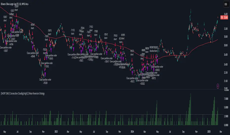
[SHORT ONLY] Consecutive Bars Above MA Strategy█ STRATEGY DESCRIPTION
The "Consecutive Bars Above MA Strategy" is a contrarian trading system aimed at exploiting overextended bullish moves in stocks and ETFs. It monitors the number of consecutive bars that close above a chosen short-term moving average (which can be either a Simple Moving Average or an Exponential Moving Average). Once the count reaches a preset threshold and the current bar’s close exceeds the previous bar’s high within a designated trading window, a short entry is initiated. An optional EMA filter further refines entries by requiring that the current close is below the 200-period EMA, helping to ensure that trades are taken in a bearish environment.
█ HOW ARE THE CONSECUTIVE BULLISH COUNTS CALCULATED?
The strategy utilizes a counter variable, `bullCount`, to track consecutive bullish bars based on their relation to the short-term moving average. Here’s how the count is determined:
Initialize the Counter
The counter is initialized at the start:
var int bullCount = na
Bullish Bar Detection
For each bar, if the close is above the selected moving average (either SMA or EMA, based on user input), the counter is incremented:
bullCount := close > signalMa ? (na(bullCount) ? 1 : bullCount + 1) : 0
Reset on Non-Bullish Condition
If the close does not exceed the moving average, the counter resets to zero, indicating a break in the consecutive bullish streak.
█ SIGNAL GENERATION
1. SHORT ENTRY
A short signal is generated when:
The number of consecutive bullish bars (i.e., bars closing above the short-term MA) meets or exceeds the defined threshold (default: 3).
The current bar’s close is higher than the previous bar’s high.
The signal occurs within the specified trading window (between Start Time and End Time).
Additionally, if the EMA filter is enabled, the entry is only executed when the current close is below the 200-period EMA.
2. EXIT CONDITION
An exit signal is triggered when the current close falls below the previous bar’s low, prompting the strategy to close the short position.
█ ADDITIONAL SETTINGS
Threshold: The number of consecutive bullish bars required to trigger a short entry (default is 3).
Trading Window: The Start Time and End Time inputs define when the strategy is active.
Moving Average Settings: Choose between SMA and EMA, and set the MA length (default is 5), which is used to assess each bar’s bullish condition.
EMA Filter (Optional): When enabled, this filter requires that the current close is below the 200-period EMA, supporting entries in a downtrend.
█ PERFORMANCE OVERVIEW
This strategy is designed for stocks and ETFs and can be applied across various timeframes.
It seeks to capture mean reversion by shorting after a series of bullish bars suggests an overextended move.
The approach employs a contrarian short entry by waiting for a breakout (close > previous high) following consecutive bullish bars.
The adjustable moving average settings and optional EMA filter allow for further optimization based on market conditions.
Comprehensive backtesting is recommended to fine-tune the threshold, moving average parameters, and filter settings for optimal performance.
[SHORT ONLY] Consecutive Close>High[1] Mean Reversion Strategy█ STRATEGY DESCRIPTION
The "Consecutive Close > High " Mean Reversion Strategy is a contrarian daily trading system for stocks and ETFs. It identifies potential shorting opportunities by counting consecutive days where the closing price exceeds the previous day's high. When this consecutive day count reaches a predetermined threshold, and if the close is below a 200-period EMA (if enabled), a short entry is triggered, anticipating a corrective pullback.
█ HOW ARE THE CONSECUTIVE BULLISH COUNTS CALCULATED?
The strategy uses a counter variable called `bullCount` to track how many consecutive bars meet a bullish condition. Here’s a breakdown of the process:
Initialize the Counter
var int bullCount = 0
Bullish Bar Detection
Every time the close exceeds the previous bar's high, increment the counter:
if close > high
bullCount += 1
Reset on Bearish Bar
When there is a clear bearish reversal, the counter is reset to zero:
if close < low
bullCount := 0
█ SIGNAL GENERATION
1. SHORT ENTRY
A Short Signal is triggered when:
The count of consecutive bullish closes (where close > high ) reaches or exceeds the defined threshold (default: 3).
The signal occurs within the specified trading window (between Start Time and End Time).
2. EXIT CONDITION
An exit Signal is generated when the current close falls below the previous bar’s low (close < low ), prompting the strategy to exit the position.
█ ADDITIONAL SETTINGS
Threshold: The number of consecutive bullish closes required to trigger a short entry (default is 3).
Start Time and End Time: The time window during which the strategy is allowed to execute trades.
EMA Filter (Optional): When enabled, short entries are only triggered if the current close is below the 200-period EMA.
█ PERFORMANCE OVERVIEW
This strategy is designed for Stocks and ETFs on the Daily timeframe and targets overextended bullish moves.
It aims to capture mean reversion by entering short after a series of consecutive bullish closes.
Further optimization is possible with additional filters (e.g., EMA, volume, or volatility).
Backtesting should be used to fine-tune the threshold and filter settings for specific market conditions.
Optimized Dynamic SupertrendDetailed Explanation of the Optimized Dynamic Supertrend Script
This Supertrend script is designed to dynamically adapt to different market conditions using ATR expansion, volume confirmation, and trend filtering. Below is a step-by-step breakdown of how it works and its functions.
1 ATR-Based Supertrend Calculation
📌 Key Purpose:
The script calculates an adaptive ATR-based Supertrend line, which acts as a dynamic support or resistance level for trend direction.
📌 How it Works:
ATR (Average True Range) is used to measure market volatility.
A dynamic ATR multiplier is applied based on price standard deviation (instead of a fixed value).
The Supertrend is calculated as:
Upper Band: SMA(close, ATR length) + (ATR Multiplier * ATR Value)
Lower Band: SMA(close, ATR length) - (ATR Multiplier * ATR Value)
The Supertrend flips when price crosses and holds beyond the Supertrend line.
🔹 Dynamic Adjustment:
Instead of using a fixed ATR multiplier, the script adjusts it using:
pinescript
Copy
Edit
dynamicFactor = ta.stdev(close, atrLength) / ta.sma(close, atrLength)
atrMultiplier = input(1.5, title="Base ATR Multiplier") * dynamicFactor
High volatility → Wider Supertrend bands (to avoid false signals).
Low volatility → Tighter Supertrend bands (for faster detection).
2 Trend Detection Logic
📌 Key Purpose:
Determines if the market is in a bullish or bearish trend based on price action.
Uses volume sensitivity and ATR expansion to reduce false signals.
📌 How it Works:
pinescript
Copy
Edit
var float supertrend = na
supertrend := close > nz(supertrend , lowerBand) ? lowerBand : upperBand
The Supertrend value updates dynamically.
If price is above the Supertrend line, the trend is bullish (green).
If price is below the Supertrend line, the trend is bearish (red).
3 Volume Sensitivity Confirmation
📌 Key Purpose:
Avoid false trend flips by confirming with volume (approximated using a CVD proxy).
📌 How it Works:
pinescript
Copy
Edit
priceChange = close - close
volumeWeightedTrend = priceChange * volume // Approximate CVD Behavior
trendConfirmed = volumeWeightedTrend > 0 ? close > supertrend : close < supertrend
Positive price change + High volume → Confirms bullish momentum.
Negative price change + High volume → Confirms bearish momentum.
If there’s low volume, the trend change is ignored to avoid false breakouts.
4 Noise Reduction (Final Trend Confirmation)
📌 Key Purpose:
Filter out weak or choppy price movements using ATR expansion.
📌 How it Works:
pinescript
Copy
Edit
trendUp = trendConfirmed and ta.atr(atrLength) > ta.atr(atrLength)
trendDown = not trendUp
Trend only flips when confirmed by volume + ATR expansion.
If ATR is not expanding, the script ignores weak price movements.
This ensures Supertrend signals align with strong market moves.
5 Can This Be Used on All Timeframes?
✅ YES! This Supertrend is adaptive, meaning it adjusts dynamically based on:
Volatility: Uses ATR expansion to adjust for different market conditions.
Timeframe Sensitivity: Works on any timeframe (1M, 5M, 15M, 1H, 4H, 1D, 1W).
Market Structure: Confirms trend flips using volume & price movement strength.
🚀 Best Timeframes for Trading:
For Scalping (1M - 15M) → Quick execution, best with order flow confirmation.
For Swing Trading (1H - 4H - 1D) → Stronger trend signals, reduced noise.
For High Timeframes (3D - 1W) → Identifies major market shifts.
🔥 Advantages & Disadvantages in Your Trading Setup
✅ Advantages:
✔ Fully Dynamic & Adaptive → Adjusts to different timeframes & volatility.
✔ Reduces False Signals → Uses ATR expansion & volume confirmation.
✔ Precise Trend Reversals → Labels LONG & SHORT entries clearly.
✔ Works on Any Market → Crypto, Forex, Stocks, Commodities.
✔ No Extra Indicators → Pure Supertrend-based (fits your setup).
❌ Disadvantages:
⚠ Lagging Indicator → ATR & volume confirmation add slight delay.
⚠ Needs High Volume to Confirm → Weak volume → no trend flip.
⚠ Choppy Market = Late Entries → Sideways movement can cause delays.
🚀 Final Thoughts:
It’s fully dynamic & adaptive (unlike traditional static Supertrends).
No extra indicators → Uses only Supertrend logic
Refines entry points using volume & ATR confirmation (removes noise).
This ensures you get high-probability trend signals while filtering out weak breakouts! 🎯
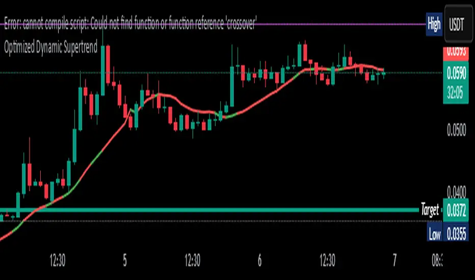
High Low Markers v1Retrieves the previous day’s high using request.security(...), so it works on any timeframe, even intraday.
Creates a single label (stored in a var variable) at that previous day high.
Places the text on the right of the anchor point by using label.style_label_right.
Updates the label’s position each bar (or only on a new day, if desired) so it always reflects the most recent previous day’s high.
Profitability Visualization with Bid-Ask Spread ApproximationOverview
The " Profitability Visualization with Bid-Ask Spread Approximation " indicator is designed to assist traders in assessing potential profit and loss targets in relation to the current market price or a simulated entry price. It provides flexibility by allowing users to choose between two methods for calculating the offset from the current price:
Bid-Ask Spread Approximation: The indicator attempts to estimate the bid-ask spread by using the highest (high) and lowest (low) prices within a given period (typically the current bar or a user-defined timeframe) as proxies for the ask and bid prices, respectively. This method provides a dynamic offset that adapts to market volatility.
Percentage Offset: Alternatively, users can specify a fixed percentage offset from the current price. This method offers a consistent offset regardless of market conditions.
Key Features
Dual Offset Calculation Methods: Choose between a dynamic bid-ask spread approximation or a fixed percentage offset to tailor the indicator to your trading style and market analysis.
Entry Price Consideration: The indicator can simulate an entry price at the beginning of each trading session (or the first bar on the chart if no sessions are defined). This feature enables a more realistic visualization of potential profit and loss levels based on a hypothetical entry point.
Profit and Loss Targets: When the entry price consideration is enabled, the indicator plots profit target (green) and loss target (red) lines. These lines represent the price levels at which a trade entered at the simulated entry price would achieve a profit or incur a loss equivalent to the calculated offset amount.
Offset Visualization: Regardless of whether the entry price is considered, the indicator always displays upper (aqua) and lower (fuchsia) offset lines. These lines represent the calculated offset levels based on the chosen method (bid-ask approximation or percentage offset).
Customization: Users can adjust the percentage offset, toggle the bid-ask approximation and entry price consideration, and customize the appearance of the lines through the indicator's settings.
Inputs
useBidAskApproximation A boolean (checkbox) input that determines whether to use the bid-ask spread approximation (true) or the percentage offset (false). Default is false.
percentageOffset A float input that allows users to specify the percentage offset to be used when useBidAskApproximation is false. The default value is 0.63.
considerEntryPrice A boolean input that enables the consideration of a simulated entry price for calculating and displaying profit and loss targets. Default is true.
Calculations
Bid-Ask Approximation (if enabled): bidApprox = request.security(syminfo.tickerid, timeframe.period, low) Approximates the bid price using the lowest price (low) of the current period. askApprox = request.security(syminfo.tickerid, timeframe.period, high) Approximates the ask price using the highest price (high) of the current period. spreadApprox = askApprox - bidApprox Calculates the approximate spread.
Offset Amount: offsetAmount = useBidAskApproximation ? spreadApprox / 2 : close * (percentageOffset / 100) Determines the offset amount based on the selected method. If useBidAskApproximation is true, the offset is half of the approximated spread; otherwise, it's the current closing price (close) multiplied by the percentageOffset.
Entry Price (if enabled): var entryPrice = 0.0 Initializes a variable to store the entry price. if considerEntryPrice Checks if entry price consideration is enabled. if barstate.isnew Checks if the current bar is the first bar of a new session. entryPrice := close Sets the entryPrice to the closing price of the first bar of the session.
Profit and Loss Targets (if entry price is considered): profitTarget = entryPrice + offsetAmount Calculates the profit target price level. lossTarget = entryPrice - offsetAmount Calculates the loss target price level.
Plotting
Profit Target Line: Plotted in green (color.green) with a dashed line style (plot.style_linebr) and increased linewidth (linewidth=2) when considerEntryPrice is true.
Loss Target Line: Plotted in red (color.red) with a dashed line style (plot.style_linebr) and increased linewidth (linewidth=2) when considerEntryPrice is true.
Upper Offset Line: Always plotted in aqua (color.aqua) to show the offset level above the current price.
Lower Offset Line: Always plotted in fuchsia (color.fuchsia) to show the offset level below the current price.
Limitations
Approximation: The bid-ask spread approximation is based on high and low prices and may not perfectly reflect the actual bid-ask spread of a specific broker, especially during periods of high volatility or low liquidity.
Simplified Entry: The entry price simulation is basic and assumes entry at the beginning of each session. It does not account for specific entry signals or order types.
No Order Execution: This indicator is purely for visualization and does not execute any trades.
Data Discrepancies: The high and low values used for approximation might not always align with real-time bid and ask prices due to differences in data aggregation and timing between TradingView and various brokers.
Disclaimer
This indicator is for educational and informational purposes only and should not be considered financial advice. Trading involves substantial risk, and past performance is not indicative of future results. Always conduct thorough research and consider your own risk tolerance before making any trading decisions. It is recommended to combine this indicator with other technical analysis tools and a well-defined trading strategy.

Heat Map Trend (VIDYA MA) [BigBeluga]The Heat Map Trend (VIDYA MA) - BigBeluga indicator is a multi-timeframe trend detection tool based on the Volumetric Variable Index Dynamic Average (VIDYA). This indicator calculates trends using volume momentum, or volatility if volume data is unavailable, and displays the trends across five customizable timeframes. It features a heat map to visualize trends, color-coded candles based on an average of the five timeframes, and a dashboard that shows the current trend direction for each timeframe. This tool helps traders identify trends while minimizing market noise and is particularly useful in detecting faster market changes in shorter timeframes.
🔵 KEY FEATURES & USAGE
◉ Volumetric Variable Index Dynamic Average (VIDYA):
The core of the indicator is the VIDYA moving average, which adjusts dynamically based on volume momentum. If volume data isn't available, the indicator uses volatility instead to smooth the moving average. This allows traders to assess the trend direction with more accuracy, using either volume or volatility, if volume data is not provided, as the basis for the trend calculation.
// VIDYA CALCULATION -----------------------------------------------------------------------------------------
// ATR (Average True Range) and volume calculation
bool volume_check = ta.cum(volume) <= 0
float atrVal = ta.atr(1)
float volVal = volume_check ? atrVal : volume // Use ATR if volume is not available
// @function: Calculate the VIDYA (Volumetric Variable Index Dynamic Average)
vidya(src, len, cmoLen) =>
float cmoVal = ta.sma(ta.cmo(volVal, cmoLen), 10) // Calculate the CMO and smooth it with an SMA
float absCmo = math.abs(cmoVal) // Absolute value of CMO
float alpha = 2 / (len + 1) // Alpha factor for smoothing
var float vidyaVal = 0.0 // Initialize VIDYA
vidyaVal := alpha * absCmo / 100 * src + (1 - alpha * absCmo / 100) * nz(vidyaVal ) // VIDYA formula
◉ Multi-Timeframe Trend Analysis with Heat Map Visualization:
The indicator calculates VIDYA across five customizable timeframes, allowing traders to analyze trends from multiple perspectives. The resulting trends are displayed as a heat map below the chart, where each timeframe is represented by a gradient color. The color intensity reflects the distance of the moving average (VIDYA) from the price, helping traders to identify trends on different timeframes visually. Shorter timeframes in the heat map are particularly useful for detecting faster market changes, while longer timeframes help to smooth out market noise and highlight the general trend.
Trend Direction:
Heat Map Reading:
◉ Dashboard for Multi-Timeframe Trend Directions:
The built-in dashboard displays the trend direction for each of the five timeframes, showing whether the trend is up or down. This quick overview provides traders with valuable insights into the current market conditions across multiple timeframes, helping them to assess whether the market is aligned or if there are conflicting trends. This allows for more informed decisions, especially during volatile periods.
◉ Color-Coded Candles Based on Multi-Timeframe Averages:
Candles are dynamically colored based on the average of the VIDYA across all five timeframes. When the price is in an uptrend, the candles are colored blue, while in a downtrend, they are colored red. If the VIDYA averages suggest a possible trend shift, the candles are displayed in orange to highlight a potential change in momentum. This color coding simplifies the process of identifying the dominant trend and spotting potential reversals.
BTC:
SP500:
◉ UP and DOWN Signals for Trend Direction Changes:
The indicator provides clear UP and DOWN signals to mark trend direction changes. When the average VIDYA crosses above a certain threshold, an UP signal is plotted, indicating a shift to an uptrend. Conversely, when it crosses below, a DOWN signal is shown, highlighting a transition to a downtrend. These signals help traders to quickly identify shifts in market direction and respond accordingly.
🔵 CUSTOMIZATION
VIDYA Length and Momentum Settings:
Adjust the length of the VIDYA moving average and the period for calculating volume momentum. These settings allow you to fine-tune how sensitive the indicator is to market changes, helping to match it with your preferred trading style.
Timeframe Selection:
Select five different timeframes to analyze trends simultaneously. This gives you the flexibility to focus on short-term trends, long-term trends, or a combination of both depending on your trading strategy.
Candle and Heat Map Color Customization:
Change the colors of the candles and heat map to fit your personal preferences. This customization allows you to align the visuals of the indicator with your overall chart setup, making it easier to analyze market conditions.
🔵 CONCLUSION
The Heat Trend (VIDYA MA) - BigBeluga indicator provides a comprehensive, multi-timeframe view of market trends, using VIDYA moving averages that adapt to volume momentum or volatility. Its heat map visualization, combined with a dashboard of trend directions and color-coded candles, makes it an invaluable tool for traders looking to understand both short-term market fluctuations and longer-term trends. By showing the overall market direction across multiple timeframes, it helps traders avoid market noise and focus on the bigger picture while being alert to faster shifts in shorter timeframes.
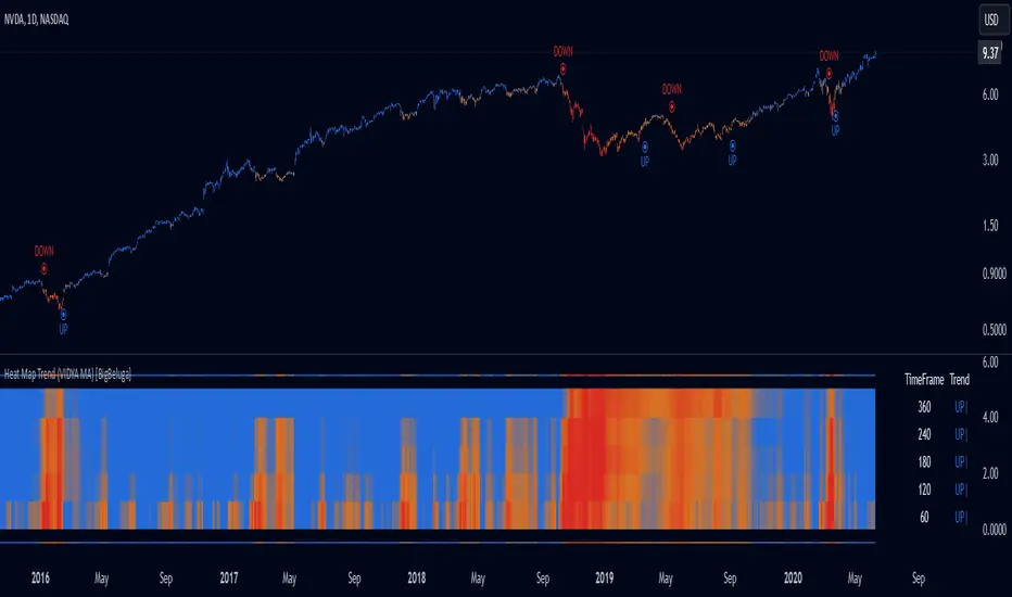
Top-Down Trend and Key Levels with Swing Points//by antaryaami0
Overview
The “Top-Down Trend and Key Levels with Swing Points” indicator is a comprehensive tool designed to enhance your technical analysis by integrating multiple trading concepts into a single, easy-to-use script. It combines higher timeframe trend analysis, key price levels, swing point detection, and ranging market identification to provide a holistic view of market conditions. This indicator is particularly useful for traders who employ multi-timeframe analysis, support and resistance levels, and price action strategies.
Key Features
1. Higher Timeframe Trend Background Shading:
• Purpose: Identifies the prevailing trend on a higher timeframe to align lower timeframe trading decisions with the broader market direction.
• How it Works: The indicator compares the current higher timeframe close with the previous one to determine if the trend is up, down, or ranging.
• Customization:
• Trend Timeframe: Set your preferred higher timeframe (e.g., Daily, Weekly).
• Up Trend Color & Down Trend Color: Customize the background colors for uptrends and downtrends.
• Ranging Market Color: A separate color to indicate when the market is moving sideways.
2. Key Price Levels:
• Previous Day High (PDH) and Low (PDL):
• Purpose: Identifies key support and resistance levels from the previous trading day.
• Visualization: Plots horizontal lines at PDH and PDL with labels.
• Customization: Option to show or hide these levels and customize their colors.
• Pre-Market High (PMH) and Low (PML):
• Purpose: Highlights the price range during the pre-market session, which can indicate potential breakout levels.
• Visualization: Plots horizontal lines at PMH and PML with labels.
• Customization: Option to show or hide these levels and customize their colors.
3. First 5-Minute Marker (F5H/F5L):
• Purpose: Marks the high or low of the first 5 minutes after the market opens, which is significant for intraday momentum.
• How it Works:
• If the first 5-minute high is above the Pre-Market High (PMH), an “F5H” label is placed at the first 5-minute high.
• If the first 5-minute high is below the PMH, an “F5L” label is placed at the first 5-minute low.
• Visualization: Labels are placed at the 9:35 AM candle (closing of the first 5 minutes), colored in purple by default.
• Customization: Option to show or hide the marker and adjust the marker color.
4. Swing Points Detection:
• Purpose: Identifies significant pivot points in price action to help recognize trends and reversals.
• How it Works: Uses left and right bars to detect pivot highs and lows, then determines if they are Higher Highs (HH), Lower Highs (LH), Higher Lows (HL), or Lower Lows (LL).
• Visualization: Plots small markers (circles) with labels (HH, LH, HL, LL) at the corresponding swing points.
• Customization: Adjust the number of left and right bars for pivot detection and the size of the markers.
5. Ranging Market Detection:
• Purpose: Identifies periods when the market is consolidating (moving sideways) within a defined price range.
• How it Works: Calculates the highest high and lowest low over a specified period and determines if the price range is within a set percentage threshold.
• Visualization: Draws a gray box around the price action during the ranging period and labels the high and low prices at the end of the range.
• Customization: Adjust the range detection period and threshold, as well as the box color.
6. Trend Coloring on Chart:
• Purpose: Provides a visual cue for the short-term trend based on a moving average.
• How it Works: Colors the candles green if the price is above the moving average and red if below.
• Customization: Set the moving average length and customize the uptrend and downtrend colors.
How to Use the Indicator
1. Adding the Indicator to Your Chart:
• Copy the Pine Script code provided and paste it into the Pine Script Editor on TradingView.
• Click “Add to Chart” to apply the indicator.
2. Configuring Inputs and Settings:
• Access Inputs:
• Click on the gear icon next to the indicator’s name on your chart to open the settings.
• Customize Key Levels:
• Show Pre-Market High/Low: Toggle on/off.
• Show Previous Day High/Low: Toggle on/off.
• Show First 5-Minute Marker: Toggle on/off.
• Set Trend Parameters:
• Trend Timeframe for Background: Choose the higher timeframe for trend analysis.
• Moving Average Length for Bar Color: Set the period for the moving average used in bar coloring.
• Adjust Ranging Market Detection:
• Range Detection Period: Specify the number of bars to consider for range detection.
• Range Threshold (%): Set the maximum percentage range for the market to be considered ranging.
• Customize Visuals:
• Colors: Adjust colors for trends, levels, markers, and ranging market boxes.
• Label Font Size: Choose the size of labels displayed on the chart.
• Level Line Width: Set the thickness of the lines for key levels.
3. Interpreting the Indicator:
• Background Shading:
• Green Shade: Higher timeframe is in an uptrend.
• Red Shade: Higher timeframe is in a downtrend.
• Gray Box: Market is ranging (sideways movement).
• Key Levels and Markers:
• PDH and PDL Lines: Represent resistance and support from the previous day.
• PMH and PML Lines: Indicate potential breakout levels based on pre-market activity.
• F5H/F5L Labels: Early indication of intraday momentum after market open.
• Swing Point Markers:
• HH (Higher High): Suggests bullish momentum.
• LH (Lower High): May indicate a potential bearish reversal.
• HL (Higher Low): Supports bullish continuation.
• LL (Lower Low): Indicates bearish momentum.
• Ranging Market Box:
• Gray Box Around Price Action: Highlights consolidation periods where breakouts may occur.
• Range High and Low Labels: Provide the upper and lower bounds of the consolidation zone.
4. Applying the Indicator to Your Trading Strategy:
• Trend Alignment:
• Use the higher timeframe trend shading to align your trades with the broader market direction.
• Key Levels Trading:
• Watch for price reactions at PDH, PDL, PMH, and PML for potential entry and exit points.
• Swing Points Analysis:
• Identify trend continuations or reversals by observing the sequence of HH, HL, LH, and LL.
• Ranging Market Strategies:
• During ranging periods, consider range-bound trading strategies or prepare for breakout trades when the price exits the range.
• Intraday Momentum:
• Use the F5H/F5L marker to gauge early market sentiment and potential intraday trends.
Practical Tips
• Adjust Settings to Your Trading Style:
• Tailor the indicator’s inputs to match your preferred timeframes and trading instruments.
• Combine with Other Indicators:
• Use in conjunction with volume indicators, oscillators, or other technical tools for additional confirmation.
• Backtesting:
• Apply the indicator to historical data to observe how it performs and refine your settings accordingly.
• Stay Updated on Market Conditions:
• Be aware of news events or economic releases that may impact market behavior and the effectiveness of technical levels.
Customization Options
• Time Zone Adjustment:
• The script uses “America/New_York” time zone by default. Adjust the timezone variable in the script if your chart operates in a different time zone.
var timezone = "Your/Timezone"
• Session Times:
• Modify the Regular Trading Session and Pre-Market Session times in the indicator settings to align with the trading hours of different markets or exchanges.
• Visual Preferences:
• Colors: Personalize the indicator’s colors to suit your visual preferences or to enhance visibility.
• Label Sizes: Adjust label sizes if you find them too intrusive or not prominent enough.
• Marker Sizes: Further reduce or enlarge the swing point markers by modifying the swing_marker_size variable.
Understanding the Indicator’s Logic
1. Higher Timeframe Trend Analysis:
• The indicator retrieves the closing prices of a higher timeframe using the request.security() function.
• It compares the current higher timeframe close with the previous one to determine the trend direction.
2. Key Level Calculation:
• Previous Day High/Low: Calculated by tracking the highest and lowest prices of the previous trading day.
• Pre-Market High/Low: Calculated by monitoring price action during the pre-market session.
3. First 5-Minute Marker Logic:
• At 9:35 AM (end of the first 5 minutes after market open), the indicator evaluates whether the first 5-minute high is above or below the PMH.
• It then places the appropriate label (F5H or F5L) on the chart.
4. Swing Points Detection:
• The script uses ta.pivothigh() and ta.pivotlow() functions to detect pivot points.
• It then determines the type of swing point based on comparisons with previous swings.
5. Ranging Market Detection:
• The indicator looks back over a specified number of bars to find the highest high and lowest low.
• It calculates the percentage difference between these two points.
• If the difference is below the set threshold, the market is considered to be ranging, and a box is drawn around the price action.
Limitations and Considerations
• Indicator Limitations:
• Maximum Boxes and Labels: Due to Pine Script limitations, there is a maximum number of boxes and labels that can be displayed simultaneously.
• Performance Impact: Adding multiple visual elements (boxes, labels, markers) can affect the performance of the script on lower-end devices or with large amounts of data.
• Market Conditions:
• False Signals: Like any technical tool, the indicator may produce false signals, especially during volatile or erratic market conditions.
• Not a Standalone Solution: This indicator should be used as part of a comprehensive trading strategy, including risk management and other forms of analysis.
Conclusion
The “Top-Down Trend and Key Levels with Swing Points” indicator is a versatile tool that integrates essential aspects of technical analysis into one script. By providing insights into higher timeframe trends, highlighting key price levels, detecting swing points, and identifying ranging markets, it equips traders with valuable information to make more informed trading decisions. Whether you are a day trader looking for intraday opportunities or a swing trader aiming to align with the broader trend, this indicator can enhance your chart analysis and trading strategy.
Disclaimer
Trading involves significant risk, and it’s important to understand that past performance is not indicative of future results. This indicator is a tool to assist in analysis and should not be solely relied upon for making trading decisions. Always conduct thorough research and consider seeking advice from financial professionals before engaging in trading activities.
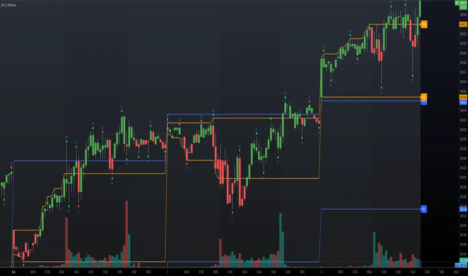
AadTrend [InvestorUnknown]The AadTrend indicator is an experimental trading tool that combines a user-selected moving average with the Average Absolute Deviation (AAD) from this moving average. This combination works similarly to the Supertrend indicator but offers additional flexibility and insights. In addition to generating Long and Short signals, the AadTrend indicator identifies RISK-ON and RISK-OFF states for each trade direction, highlighting areas where taking on more risk may be considered.
Core Concepts and Features
Moving Average (User-Selected Type)
The indicator allows users to select from various types of moving averages to suit different trading styles and market conditions:
Simple Moving Average (SMA)
Exponential Moving Average (EMA)
Hull Moving Average (HMA)
Double Exponential Moving Average (DEMA)
Triple Exponential Moving Average (TEMA)
Relative Moving Average (RMA)
Fractal Adaptive Moving Average (FRAMA)
Average Absolute Deviation (AAD)
The Average Absolute Deviation measures the average distance between each data point and the mean, providing a robust estimation of volatility.
aad(series float src, simple int length, simple string avg_type) =>
avg = // Moving average as selected by the user
abs_deviations = math.abs(src - avg)
ta.sma(abs_deviations, length)
This provides a volatility measure that adapts to recent market conditions.
Combining Moving Average and AAD
The indicator creates upper and lower bands around the moving average using the AAD, similar to how the Supertrend indicator uses Average True Range (ATR) for its bands.
AadTrend(series float src, simple int length, simple float aad_mult, simple string avg_type) =>
// Calculate AAD (volatility measure)
aad_value = aad(src, length, avg_type)
// Calculate the AAD-based moving average by scaling the price data with AAD
avg = switch avg_type
"SMA" => ta.sma(src, length)
"EMA" => ta.ema(src, length)
"HMA" => ta.hma(src, length)
"DEMA" => ta.dema(src, length)
"TEMA" => ta.tema(src, length)
"RMA" => ta.rma(src, length)
"FRAMA" => ta.frama(src, length)
avg_p = avg + (aad_value * aad_mult)
avg_m = avg - (aad_value * aad_mult)
var direction = 0
if ta.crossover(src, avg_p)
direction := 1
else if ta.crossunder(src, avg_m)
direction := -1
A chart displaying the moving average with upper and lower AAD bands enveloping the price action.
Signals and Trade States
1. Long and Short Signals
Long Signal: Generated when the price crosses above the upper AAD band,
Short Signal: Generated when the price crosses below the lower AAD band.
2. RISK-ON and RISK-OFF States
These states provide additional insight into the strength of the current trend and potential opportunities for taking on more risk.
RISK-ON Long: When the price moves significantly above the upper AAD band after a Long signal.
RISK-OFF Long: When the price moves back below the upper AAD band, suggesting caution.
RISK-ON Short: When the price moves significantly below the lower AAD band after a Short signal.
RISK-OFF Short: When the price moves back above the lower AAD band.
Highlighted areas on the chart representing RISK-ON and RISK-OFF zones for both Long and Short positions.
A chart showing the filled areas corresponding to trend directions and RISK-ON zones
Backtesting and Performance Metrics
While the AadTrend indicator focuses on generating signals and highlighting risk areas, it can be integrated with backtesting frameworks to evaluate performance over historical data.
Integration with Backtest Library:
import InvestorUnknown/BacktestLibrary/1 as backtestlib
Customization and Calibration
1. Importance of Calibration
Default Settings Are Experimental: The default parameters are not optimized for any specific market condition or asset.
User Calibration: Traders should adjust the length, aad_mult, and avg_type parameters to align the indicator with their trading strategy and the characteristics of the asset being analyzed.
2. Factors to Consider
Market Volatility: Higher volatility may require adjustments to the aad_mult to avoid false signals.
Trading Style: Short-term traders might prefer faster-moving averages like EMA or HMA, while long-term traders might opt for SMA or FRAMA.
Alerts and Notifications
The AadTrend indicator includes built-in alert conditions to notify traders of significant market events:
Long and Short Alerts:
alertcondition(long_alert, "LONG (AadTrend)", "AadTrend flipped ⬆LONG⬆")
alertcondition(short_alert, "SHORT (AadTrend)", "AadTrend flipped ⬇Short⬇")
RISK-ON and RISK-OFF Alerts:
alertcondition(risk_on_long, "RISK-ON LONG (AadTrend)", "RISK-ON LONG (AadTrend)")
alertcondition(risk_off_long, "RISK-OFF LONG (AadTrend)", "RISK-OFF LONG (AadTrend)")
alertcondition(risk_on_short, "RISK-ON SHORT (AadTrend)", "RISK-ON SHORT (AadTrend)")
alertcondition(risk_off_short, "RISK-OFF SHORT (AadTrend)", "RISK-OFF SHORT (AadTrend)")
Important Notes and Disclaimer
Experimental Nature: The AadTrend indicator is experimental and should be used with caution.
No Guaranteed Performance: Past performance is not indicative of future results. Backtesting results may not reflect real trading conditions.
User Responsibility: Traders and investors should thoroughly test and calibrate the indicator settings before applying it to live trading.
Risk Management: Always use proper risk management techniques, including stop-loss orders and position sizing.

Prometheus Markov ChainThe Prometheus Markov Chain Indicator is a custom-built tool designed to predict potential future price movements using a Markov Chain approach. A Markov Chain is a statistical model that assumes the probability of moving to a future state depends solely on the current state. In this indicator, states represent price movement classifications—bullish, bearish, or neutral—and are determined based on historical price changes (percentage returns). The indicator builds a transition matrix to calculate probabilities of transitioning from one state to another, enabling traders to identify patterns and forecast likely price actions.
Core Functionality and Transition Matrix
The transition matrix is the backbone of the Markov Chain. It captures the frequency of transitions between states in the historical price data and normalizes these counts into probabilities. For example, if the price was in a bearish state and transitioned to a bullish state 3 out of 10 times, the probability of transitioning from bearish to bullish would be 0.3. The matrix is created dynamically using the stateFunc function to classify states, which can use either dynamic thresholds (highest and lowest returns over a lookback period) or a user-defined percent return threshold. Below is the snippet that updates the transition matrix:
transitionMatrix = matrix.new(dimension, dimension, 0.0)
for i = 0 to array.size(vec) - 2
fromState = array.get(vec, i)
toState = array.get(vec, i + 1)
transitionMatrix.set(fromState, toState, transitionMatrix.get(fromState, toState) + 1)
for i = 0 to dimension - 1
rowSum = 0.0
for j = 0 to dimension - 1
rowSum += transitionMatrix.get(i, j)
for j = 0 to dimension - 1
prob = transitionMatrix.get(i, j) / rowSum
transitionMatrix.set(i, j, prob)
This snippet iterates through historical price movements, counts state transitions, and then normalizes each row of the matrix so that the sum of probabilities for all possible transitions from a given state equals 1.
How the Indicator Predicts Future States
After constructing the transition matrix, the indicator calculates the current state of the price based on the latest percentage return and then uses the matrix to compute probabilities for transitioning to other states. The state with the highest probability is predicted as the next state, which is displayed on the chart using color-coded labels: green for bullish and red for bearish. The following snippet demonstrates how the current state and predictions are calculated:
current_chng = (close - close ) / close
var int current_state = na
if not use_custom_thresh
highest_chng = ta.highest(current_chng, int(size) * 2)
lowest_chng = ta.lowest(current_chng, int(size) * 2)
current_state := stateFunc(current_chng, highest_chng, lowest_chng)
else
current_state := stateFunc(current_chng, custom_thresh)
predicted_probs = array.new(dimension, 0.0)
for j = 0 to dimension - 1
array.set(predicted_probs, j, transitionMatrix.get(current_state, j))
The indicator evaluates which state has the highest transition probability (highest_prob) and places corresponding labels on the chart. For example, if the next state is predicted to be bullish, a green "Bullish" label is placed below the current bar. This predictive functionality helps traders anticipate potential reversals or continuations in price trends based on historical behavior patterns.
Usage:
Here we see the indicator at work on $PLTR. The states predicted are bullish then bearish. In this example we then see price move in a way that verifies those predictions.
On this 4 Hour NASDAQ:AMZN chart we see predictions play out in a short trade style. States quickly move from one to another but not without giving traders a way to take advantage.
This is the perspective we aim to provide. We encourage traders to not follow indicators blindly. No indicator is 100% accurate. This one can give you a different perspective market state. We encourage any comments about desired updates or criticism!

hinton_map█ HINTON MAP
This library provides functions to create and display a Hinton Map visualization. A Hinton map uses squares to represent the magnitude and direction of values in a matrix. This library allows you to display multiple ticker/timeframe/indicator combinations on a single chart, using color/boxsize/bnordersize to represent the values used. The values must be from -1.0 to 1.0 in value. 3 different values can be input per square.
Example Usage:
The example below demonstrates how to create a Hinton Map for two symbols (AAPL and MSFT) across three timeframes (1 minute, 5 minutes, and 1 day).
var hintonData = hinton_map.initHintonData(2, 3)
tickers = array.from("AAPL", "MSFT")
timeframes = array.from("1", "5", "1D")
for i = 0 to array.size(tickers) - 1
for j = 0 to array.size(timeframes) - 1
ticker = array.get(tickers, i)
timeframe = array.get(timeframes, j)
= request.security(ticker, timeframe, [close, close , ta.rsi(close, 14)], lookahead = barmerge.lookahead_on)
percent_change = (close_current - close_previous) / close_previous * 100
rsi_deviation = rsi_current - 50
hintonData.unitMatrix.set(i, j, hinton_map.createHintonUnit(
fillValue = percent_change,
borderValue = rsi_deviation,
innerValue = percent_change * rsi_deviation,
boxText = dv.from_string(str.tostring(math.round(percent_change, 2)) + "%"),
tooltipText = dv.from_string(syminfo.ticker + ", " + timeframe + ": " + str.tostring(math.round(percent_change, 2)) + "%, RSI: " + str.tostring(math.round(rsi_current, 2)))
))
hinton_map.drawHintonMap(hintonData)
█ createHintonUnit
Creates a Hinton unit.
• fillValue
Value to determine the fill color hue.
Type: float
Default Value: 0.0
• borderValue
Value to determine the border color hue and width.
Type: float
Default Value: 0.0
• innerValue
Value to determine the inner box color hue.
Type: float
Default Value: 0.0
• boxText
Text to display in the inner box.
Type: dv.DisplayValue
Default Value: na
• tooltipText
Tooltip text for the inner box.
Type: dv.DisplayValue
Default Value: na
Returns: HintonUnit
█ initHintonData
Initializes Hinton map data structure.
• rows
Number of rows.
Type: int
• columns
Number of columns.
Type: int
Returns: HintonData
█ drawHintonMap
Draws a Hinton map.
• hintonData
Hinton map data.
Type: HintonData
• unitSize
Size of each unit in bars.
Type: int
Default Value: 10
• borderWidth
Base width of the inner box border.
Type: int
Default Value: 5
• plusHue
Hue value for positive values (0-360).
Type: float
Default Value: 180
• minusHue
Hue value for negative values (0-360).
Type: float
Default Value: -30
█ HintonUnit
Data for a Hinton unit.
• fillValue
Value to determine the fill color hue.
Type: float
• borderValue
Value to determine the border color hue and width.
Type: float
• innerValue
Value to determine the inner box color hue.
Type: float
• boxText
Text to display in the inner box.
Type: dv.DisplayValue
• tooltipText
Tooltip text for the inner box.
Type: dv.DisplayValue
█ HintonData
Structure to store Hinton map data.
• unitMatrix
Matrix of Hinton units.
Type: matrix
• lineMatrix
Matrix of lines.
Type: matrix
• labelMatrix
Matrix of labels.
Type: matrix
• boxMatrix
Matrix of boxes.
Type: matrix
• fillMatrix
Matrix of line fills.
Type: matrix
MadTrend [InvestorUnknown]The MadTrend indicator is an experimental tool that combines the Median and Median Absolute Deviation (MAD) to generate signals, much like the popular Supertrend indicator. In addition to identifying Long and Short positions, MadTrend introduces RISK-ON and RISK-OFF states for each trade direction, providing traders with nuanced insights into market conditions.
Core Concepts
Median and Median Absolute Deviation (MAD)
Median: The middle value in a sorted list of numbers, offering a robust measure of central tendency less affected by outliers.
Median Absolute Deviation (MAD): Measures the average distance between each data point and the median, providing a robust estimation of volatility.
Supertrend-like Functionality
MadTrend utilizes the median and MAD in a manner similar to how Supertrend uses averages and volatility measures to determine trend direction and potential reversal points.
RISK-ON and RISK-OFF States
RISK-ON: Indicates favorable conditions for entering or holding a position in the current trend direction.
RISK-OFF: Suggests caution, signaling RISK-ON end and potential trend weakening or reversal.
Calculating MAD
The mad function calculates the median of the absolute deviations from the median, providing a robust measure of volatility.
// Function to calculate the Median Absolute Deviation (MAD)
mad(series float src, simple int length) =>
med = ta.median(src, length) // Calculate median
abs_deviations = math.abs(src - med) // Calculate absolute deviations from median
ta.median(abs_deviations, length) // Return the median of the absolute deviations
MADTrend Function
The MADTrend function calculates the median and MAD-based upper (med_p) and lower (med_m) bands. It determines the trend direction based on price crossing these bands.
MADTrend(series float src, simple int length, simple float mad_mult) =>
// Calculate MAD (volatility measure)
mad_value = mad(close, length)
// Calculate the MAD-based moving average by scaling the price data with MAD
median = ta.median(close, length)
med_p = median + (mad_value * mad_mult)
med_m = median - (mad_value * mad_mult)
var direction = 0
if ta.crossover(src, med_p)
direction := 1
else if ta.crossunder(src, med_m)
direction := -1
Trend Direction and Signals
Long Position (direction = 1): When the price crosses above the upper MAD band (med_p).
Short Position (direction = -1): When the price crosses below the lower MAD band (med_m).
RISK-ON: When the price moves further in the direction of the trend (beyond median +- MAD) after the initial signal.
RISK-OFF: When the price retraces towards the median, signaling potential weakening of the trend.
RISK-ON and RISK-OFF States
RISK-ON LONG: Price moves above the upper band after a Long signal, indicating strengthening bullish momentum.
RISK-OFF LONG: Price falls back below the upper band, suggesting potential weakness in the bullish trend.
RISK-ON SHORT: Price moves below the lower band after a Short signal, indicating strengthening bearish momentum.
RISK-OFF SHORT: Price rises back above the lower band, suggesting potential weakness in the bearish trend.
Picture below show example RISK-ON periods which can be identified by “cloud”
Note: Highlighted areas on the chart indicating RISK-ON and RISK-OFF periods for both Long and Short positions.
Implementation Details
Inputs and Parameters:
Source (input_src): The price data used for calculations (e.g., close, open, high, low).
Median Length (length): The number of periods over which the median and MAD are calculated.
MAD Multiplier (mad_mult): Determines the distance of the upper and lower bands from the median.
Calculations:
Median and MAD are recalculated each period based on the specified length.
Upper (med_p) and Lower (med_m) Bands are computed by adding and subtracting the scaled MAD from the median.
Visual representation of the indicator on a price chart:
Backtesting and Performance Metrics
The MadTrend indicator includes a Backtesting Mode with a performance metrics table to evaluate its effectiveness compared to a simple buy-and-hold strategy.
Equity Calculation:
Calculates the equity curve based on the signals generated by the indicator.
Performance Metrics:
Metrics such as Mean Returns, Standard Deviation, Sharpe Ratio, Sortino Ratio, and Omega Ratio are computed.
The metrics are displayed in a table for both the strategy and the buy-and-hold approach.
Note: Due to the use of labels and plot shapes, automatic chart scaling may not function ideally in Backtest Mode.
Alerts and Notifications
MadTrend provides alert conditions to notify traders of significant events:
Trend Change Alerts
RISK-ON and RISK-OFF Alerts - Provides real-time notifications about the RISK-ON and RISK-OFF states for proactive trade management.
Customization and Calibration
Default Settings: The provided default settings are experimental and not optimized. They serve as a starting point for users.
Parameter Adjustment: Traders are encouraged to calibrate the indicator's parameters (e.g., length, mad_mult) to suit their specific trading style and the characteristics of the asset being analyzed.
Source Input: The indicator allows for different price inputs (open, high, low, close, etc.), offering flexibility in how the median and MAD are calculated.
Important Notes
Market Conditions: The effectiveness of the MadTrend indicator can vary across different market conditions. Regular calibration is recommended.
Backtest Limitations: Backtesting results are historical and do not guarantee future performance.
Risk Management: Always apply sound risk management practices when using any trading indicator.

Patrick [TFO]This Patrick indicator was made for the 1 year anniversary of my Spongebob indicator, which was an experiment in using the polyline features of Pine Script to draw complex subjects. This indicator was made with the same methodology, with some helper functions to make things a bit easier on myself. It's sole purpose is to display a picture of Patrick Star on your chart, particularly the "I have $3" meme.
The initial Spongebob indicator included more than 1300 lines of code, as there were several more shapes to account for compared to Patrick, however it was done rather inefficiently. I essentially used an anchor point for each "layer" or shape (eye, nose, mouth, etc.), and drew from that point. This resulted in a ton of trial and error as I had to be very careful about the anchor points for each and every layer, and then draw around that point. In this indicator, however, I gave myself a frame to work with by specifying fixed bounds that you'll see in the code: LEFT, RIGHT, TOP, and BOTTOM.
var y_size = 4
atr = ta.atr(50)
LEFT = bar_index + 10
RIGHT = LEFT + 200
TOP = open + atr * y_size
BOTTOM = open - atr * y_size
You may notice that the top and bottom scale with the atr, or Average True Range to account for varying price fluctuations on different assets.
With these limits established, I could write some simple functions to translate my coordinates, using a range of 0-100 to describe how far the X coordinates should be from left to right, where left is 0 and right is 100; and likewise how far the Y coordinates should be from bottom to top, where bottom is 0 and top is 100.
X(float P) =>
result = LEFT + math.floor((RIGHT - LEFT)*P/100)
Y(float P) =>
result = BOTTOM + (TOP - BOTTOM)*P/100
With these functions, I could then start drawing points much simpler, with respect to the overall frame of the picture. If I wanted a point in the dead center of the frame, I would choose X(50), Y(50) for example.
At this point, the process just became tediously drawing each layer of my reference picture, including but not limited to Patrick's body, arm, mouth, eyes, eyebrows, etc. I've attached the reference picture here (left), without the text enabled.
As tedious as this was to create, it was done much more efficiently than Spongebob, and the ideas used here will make it much easier to draw more complex subjects in the future.

FibExtender [tradeviZion]FibExtender : A Guide to Identifying Resistance with Fibonacci Levels
Introduction
Fibonacci levels are essential tools in technical analysis, helping traders identify potential resistance and support zones in trending markets. FibExtender is designed to make this analysis accessible to traders at all levels, especially beginners, by automating the process of plotting Fibonacci extensions. With FibExtender, you can visualize potential resistance levels quickly, empowering you to make more informed trading decisions without manually identifying every pivot point. In this article, we’ll explore how FibExtender works, guide you step-by-step in using it, and share insights for both beginner and advanced users.
What is FibExtender ?
FibExtender is an advanced tool that automates Fibonacci extension plotting based on significant pivot points in price movements. Fibonacci extensions are percentages based on prior price swings, often used to forecast potential resistance zones where price might reverse or consolidate. By automatically marking these Fibonacci levels on your chart, FibExtender saves time and reduces the complexity of technical analysis, especially for users unfamiliar with calculating and plotting these levels manually.
FibExtender not only identifies Fibonacci levels but also provides a customizable framework where you can adjust anchor points, colors, and level visibility to suit your trading strategy. This customization allows traders to tailor the indicator to fit different market conditions and personal preferences.
Key Features of FibExtender
FibExtender offers several features to make Fibonacci level analysis easier and more effective. Here are some highlights:
Automated Fibonacci Level Identification : The script automatically detects recent swing lows and pivot points to anchor Fibonacci extensions, allowing you to view potential resistance levels with minimal effort.
Customizable Fibonacci Levels : Users can adjust the specific Fibonacci levels they want to display (e.g., 0.618, 1.0, 1.618), enabling a more focused analysis based on preferred ratios. Each level can be color-coded for visual clarity.
Dual Anchor Points : FibExtender allows you to choose between anchoring levels from either the last pivot low or a recent swing low, depending on your preference. This flexibility helps in aligning Fibonacci levels with key market structures.
Transparency and Visual Hierarchy : FibExtender automatically adjusts the transparency of levels based on their "sequence age," creating a subtle visual hierarchy. Older levels appear slightly faded, helping you focus on more recent, potentially impactful levels.
Connection Lines for Context : FibExtender draws connecting lines from recent lows to pivot highs, allowing users to visualize the price movements that generated each Fibonacci extension level.
Step-by-Step Guide for Beginners
Let’s walk through how to use the FibExtender script on a TradingView chart. This guide will ensure that you’re able to set it up and interpret the key information displayed by the indicator.
Step 1: Adding FibExtender to Your Chart
Open your TradingView chart and select the asset you wish to analyze.
Search for “FibExtender ” in the Indicators section.
Click to add the indicator to your chart, and it will automatically plot Fibonacci levels based on recent pivot points.
Step 2: Customizing Fibonacci Levels
Adjust Levels : Under the "Fibonacci Settings" tab, you can enable or disable specific levels, such as 0.618, 1.0, or 1.618. You can also change the color for each level to improve visibility.
Set Anchor Points : Choose between "Last Pivot Low" and "Recent Swing Low" as your Fibonacci anchor point. If you want a broader view, choose "Recent Swing Low"; if you prefer tighter levels, "Last Pivot Low" may be more suitable.
Fib Line Length : Modify the line length for Fibonacci levels to make them more visible on your chart.
Step 3: Spotting Visual Clusters (Manual Analysis)
Identify Potential Resistance Clusters : Look for areas on your chart where multiple Fibonacci levels appear close together. For example, if you see 1.0, 1.272, and 1.618 levels clustered within a small price range, this may indicate a stronger resistance zone.
Why Clusters Matter : Visual clusters often signify areas where traders expect heightened price reaction. When levels are close, it suggests that resistance may be reinforced by multiple significant ratios, making it harder for price to break through. Use these clusters to anticipate potential pullbacks or consolidation areas.
Step 4: Observing the Price Action Around Fibonacci Levels
As price approaches these identified levels, watch for any slowing momentum or reversal patterns, such as doji candles or bearish engulfing formations, that might confirm resistance.
Adjust Strategy Based on Resistance : If price hesitates or reverses at a clustered resistance zone, it may be a signal to secure profits or tighten stops on a long position.
Advanced Insights (for Intermediate to Advanced Users)
For users interested in the technical workings of FibExtender, this section provides insights into how the indicator functions on a code level.
Pivot Point and Swing Detection
FibExtender uses a pivot-high and pivot-low detection function to identify significant price points. The upFractal and dnFractal variables detect these levels based on recent highs and lows, creating the basis for Fibonacci extension calculations. Here’s an example of the code used for this detection:
// Fractal Calculations
upFractal = ta.pivothigh(n, n)
dnFractal = ta.pivotlow(n, n)
By setting the number of periods for n, users can adjust the sensitivity of the script to recent price swings.
Fibonacci Level Calculation
The following function calculates the Fibonacci levels based on the selected pivot points and applies each level’s specific ratio (e.g., 0.618, 1.618) to project extensions above the recent price swing.
calculateFibExtensions(float startPrice, float highPrice, float retracePrice) =>
fibRange = highPrice - startPrice
var float levels = array.new_float(0)
array.clear(levels)
if array.size(fibLevels) > 0
for i = 0 to array.size(fibLevels) - 1
level = retracePrice + (fibRange * array.get(fibLevels, i))
array.push(levels, level)
levels
This function iterates over each level enabled by the user, calculating extensions by multiplying the price range by the corresponding Fibonacci ratio.
Example Use Case: Identifying Resistance in Microsoft (MSFT)
To better understand how FibExtender highlights resistance, let’s look at Microsoft’s stock chart (MSFT), as shown in the image. The chart displays several Fibonacci levels extending upward from a recent pivot low around $408.17. Here’s how you can interpret the chart:
Clustered Resistance Levels : In the chart, note the grouping of several Fibonacci levels in the range of $450–$470. These levels, particularly when tightly packed, suggest a zone where Microsoft may encounter stronger resistance, as multiple Fibonacci levels signal potential barriers.
Applying Trading Strategies : As price approaches this clustered resistance, traders can watch for weakening momentum. If price begins to stall, it may be wise to lock in profits on long positions or set tighter stop-loss orders.
Observing Momentum Reversals : Look for specific candlestick patterns as price nears these levels, such as bearish engulfing candles or doji patterns. Such patterns can confirm resistance, helping you make informed decisions on whether to exit or manage your position.
Conclusion: Harnessing Fibonacci Extensions with FibExtender
FibExtender is a powerful tool for identifying potential resistance levels without the need for manual Fibonacci calculations. It automates the detection of key swing points and projects Fibonacci extensions, offering traders a straightforward approach to spotting potential resistance zones. For beginners, FibExtender provides a user-friendly gateway to technical analysis, helping you visualize levels where price may react.
For those with a bit more experience, the indicator offers insight into pivot points and Fibonacci calculations, enabling you to fine-tune the analysis for different market conditions. By carefully observing price reactions around clustered levels, users can identify areas of stronger resistance and refine their trade management strategies accordingly.
FibExtender is not just a tool but a framework for disciplined analysis. Using Fibonacci levels for guidance can support your trading decisions, helping you recognize areas where price might struggle or reverse. Integrating FibExtender into your trading strategy can simplify the complexity of Fibonacci extensions and enhance your understanding of resistance dynamics.
Note: Always practice proper risk management and thoroughly test the indicator to ensure it aligns with your trading strategy. Past performance is not indicative of future results.
Trade smarter with TradeVizion—unlock your trading potential today!