Pinescript v3 Compatibility Framework (v4 Migration Tool)Pinescript v3 Compatibility Framework (v4 Migration Tool)
This code makes most v3 scripts work in v4 with only a few minor changes below. Place the framework code before the first input statement.
You can totally delete all comments.
Pros:
- to port to v4 you only need to make a few simple changes, not affecting the core v3 code functionality
Cons:
- without #include - large redundant code block, but can be reduced as needed
- no proper syntax highlighting, intellisence for substitute constant names
Make the following changes in v3 script:
1. standard types can't be var names, color_transp can't be in a function, rename in v3 script:
color() => color.new()
bool => bool_
integer => integer_
float => float_
string => string_
2. init na requires explicit type declaration
float a = na
color col = na
3. persistent var init (optional):
s = na
s := nz(s , s) // or s := na(s ) ? 0 : s
// can be replaced with var s
var s = 0
s := s + 1
___________________________________________________________
Key features of Pinescript v4 (FYI):
1. optional explicit type declaration/conversion (you still can't cast series to int)
float s
2. persistent var modifier
var s
var float s
3. string series - persistent strings now can be used in cond and output to screen dynamically
4. label and line objects
- can be dynamically created, deleted, modified using get/set functions, moved before/after the current bar
- can be in if or a function unlike plot
- max limit: 50-55 label, and 50-55 line drawing objects in addition to already existing plots - both not affected by max plot outputs 64
- can only be used in the main chart
- can serve as the only output function - at least one is required: plot, barcolor, line, label etc.
- dynamic var values (including strings) can be output to screen as text using label.new and to_string
str = close >= open ? "up" : "down"
label.new(bar_index, high, text=str)
col = close >= open ? color.green : color.red
label.new(bar_index, na, "close = " + tostring(close), color=col, textcolor=color.white, style=label.style_labeldown, yloc=yloc.abovebar)
// create new objects, delete old ones
l = line.new(bar_index, high, bar_index , low , width=4)
line.delete(l )
// free object buffer by deleting old objects first, then create new ones
var l = na
line.delete(l)
l = line.new(bar_index, high, bar_index , low , width=4)
Komut dosyalarını "VAR+计量模型+黄金期货" için ara

footprint_typeLibrary "footprint_type"
Contains all types for calculating and rendering footprints
Inputs
Inputs objects
Fields:
inbalance_percent (series int) : percentage coefficient to determine the Imbalance of price levels
stacked_input (series int) : minimum number of consecutive Imbalance levels required to draw extended lines
show_summary_footprint (series bool) : bool input for show summary footprint
procent_volume_area (series int) : definition size Value area
show_vah (series bool) : bool input for show VAH
show_poc (series bool) : bool input for show POC
show_val (series bool) : bool input for show VAL
color_vah (series color) : color VAH line
color_poc (series color) : color POC line
color_val (series color) : color VAL line
show_volume_profile (series bool)
new_imbalance_cond (series bool) : bool input for setup alert on new imbalance buy and sell
new_imbalance_line_cond (series bool) : bool input for setup alert on new imbalance line buy and sell
stop_past_imbalance_line_cond (series bool) : bool input for setup alert on stop past imbalance line buy and sell
Constants
Constants all Constants objects
Fields:
imbalance_high_char (series string) : char for printing buy imbalance
imbalance_low_char (series string) : char for printing sell imbalance
color_title_sell (series color) : color for footprint sell
color_title_buy (series color) : color for footprint buy
color_line_sell (series color) : color for sell line
color_line_buy (series color) : color for buy line
color_title_none (series color) : color None
Calculation_data
Calculation_data data for calculating
Fields:
detail_open (array) : array open from calculation timeframe
detail_high (array) : array high from calculation timeframe
detail_low (array) : array low from calculation timeframe
detail_close (array) : array close from calculation timeframe
detail_vol (array) : array volume from calculation timeframe
previos_detail_close (array) : array close from calculation timeframe
isBuyVolume (series bool) : attribute previosly bar buy or sell
Footprint_row
Footprint_row objects one footprint row
Fields:
price (series float) : row price
buy_vol (series float) : buy volume
sell_vol (series float) : sell volume
imbalance_buy (series bool) : attribute buy inbalance
imbalance_sell (series bool) : attribute sell imbalance
buy_vol_box (series box) : for ptinting buy volume
sell_vol_box (series box) : for printing sell volume
buy_vp_box (series box) : for ptinting volume profile buy
sell_vp_box (series box) : for ptinting volume profile sell
row_line (series label) : for ptinting row price
empty (series bool) : = true attribute row with zero volume buy and zero volume sell
Value_area
Value_area objects for calculating and printing Value area
Fields:
vah_price (series float) : VAH price
poc_price (series float) : POC price
val_price (series float) : VAL price
vah_label (series label) : label for VAH
poc_label (series label) : label for POC
val_label (series label) : label for VAL
vah_line (series line) : line for VAH
poc_level (series line) : line for POC
val_line (series line) : line for VAL
Imbalance_line_var_object
Imbalance_line_var_object var objects printing and calculation imbalance line
Fields:
cum_buy_line (array) : line array for saving all history buy imbalance line
cum_sell_line (array) : line array for saving all history sell imbalance line
Imbalance_line
Imbalance_line objects printing and calculation imbalance line
Fields:
buy_price_line (array) : float array for saving buy imbalance price level
sell_price_line (array) : float array for saving sell imbalance price level
var_imba_line (Imbalance_line_var_object) : var objects this type
Footprint_info_var_object
Footprint_info_var_object var objects for info printing
Fields:
cum_delta (series float) : var delta volume
cum_total (series float) : var total volume
cum_buy_vol (series float) : var buy volume
cum_sell_vol (series float) : var sell volume
cum_info (series table) : table for ptinting
Footprint_info
Footprint_info objects for info printing
Fields:
var_info (Footprint_info_var_object) : var objects this type
total (series label) : total volume
delta (series label) : delta volume
summary_label (series label) : label for ptinting
Footprint_bar
Footprint_bar all objects one bar with footprint
Fields:
foot_rows (array) : objects one row footprint
val_area (Value_area) : objects Value area
imba_line (Imbalance_line) : objects imbalance line
info (Footprint_info) : objects info - table,label and their variable
row_size (series float) : size rows
total_vol (series float) : total volume one footprint bar
foot_buy_vol (series float) : buy volume one footprint bar
foot_sell_vol (series float) : sell volume one footprint bar
foot_max_price_vol (map) : map with one value - price row with max volume buy + sell
calc_data (Calculation_data) : objects with detail data from calculation resolution
Support_objects
Support_objects support object for footprint calculation
Fields:
consts (Constants) : all consts objects
inp (Inputs) : all input objects
bar_index_show_condition (series bool) : calculation bool value for show all objects footprint
row_line_color (series color) : calculation value - color for row price

Polyline PlusThis library introduces the `PolylinePlus` type, which is an enhanced version of the built-in PineScript `polyline`. It enables two features that are absent from the built-in type:
1. Developers can now efficiently add or remove points from the polyline. In contrast, the built-in `polyline` type is immutable, requiring developers to create a new instance of the polyline to make changes, which is cumbersome and incurs a significant performance penalty.
2. Each `PolylinePlus` instance can theoretically hold up to ~1M points, surpassing the built-in `polyline` type's limit of 10K points, as long as it does not exceed the memory limit of the PineScript runtime.
Internally, each `PolylinePlus` instance utilizes an array of `line`s and an array of `polyline`s. The `line`s array serves as a buffer to store lines formed by recently added points. When the buffer reaches its capacity, it flushes the contents and converts the lines into polylines. These polylines are expected to undergo fewer updates. This approach is similiar to the concept of "Buffered I/O" in file and network systems. By connecting the underlying lines and polylines, this library achieves an enhanced polyline that is dynamic, efficient, and capable of surpassing the maximum number of points imposed by the built-in polyline.
🔵 API
Step 1: Import this library
import algotraderdev/polylineplus/1 as pp
// remember to check the latest version of this library and replace the 1 above.
Step 2: Initialize the `PolylinePlus` type.
var p = pp.PolylinePlus.new()
There are a few optional params that developers can specify in the constructor to modify the behavior and appearance of the polyline instance.
var p = pp.PolylinePlus.new(
// If true, the drawing will also connect the first point to the last point, resulting in a closed polyline.
closed = false,
// Determines the field of the chart.point objects that the polyline will use for its x coordinates. Either xloc.bar_index (default), or xloc.bar_time.
xloc = xloc.bar_index,
// Color of the polyline. Default is blue.
line_color = color.blue,
// Style of the polyline. Default is line.style_solid.
line_style = line.style_solid,
// Width of the polyline. Default is 1.
line_width = 1,
// The maximum number of points that each built-in `polyline` instance can contain.
// NOTE: this is not to be confused with the maximum of points that each `PolylinePlus` instance can contain.
max_points_per_builtin_polyline = 10000,
// The number of lines to keep in the buffer. If more points are to be added while the buffer is full, then all the lines in the buffer will be flushed into the poylines.
// The higher the number, the less frequent we'll need to // flush the buffer, and thus lead to better performance.
// NOTE: the maximum total number of lines per chart allowed by PineScript is 500. But given there might be other places where the indicator or strategy are drawing lines outside this polyline context, the default value is 50 to be safe.
lines_bffer_size = 50)
Step 3: Push / Pop Points
// Push a single point
p.push_point(chart.point.now())
// Push multiple points
chart.point points = array.from(p1, p2, p3) // Where p1, p2, p3 are all chart.point type.
p.push_points(points)
// Pop point
p.pop_point()
// Resets all the points in the polyline.
p.set_points(points)
// Deletes the polyline.
p.delete()
🔵 Benchmark
Below is a simple benchmark comparing the performance between `PolylinePlus` and the native `polyline` type for incrementally adding 10K points to a polyline.
import algotraderdev/polylineplus/2 as pp
var t1 = 0
var t2 = 0
if bar_index < 10000
int start = timenow
var p = pp.PolylinePlus.new(xloc = xloc.bar_time, closed = true)
p.push_point(chart.point.now())
t1 += timenow - start
start := timenow
var polyline pl = na
var points = array.new()
points.push(chart.point.now())
if not na(pl)
pl.delete()
pl := polyline.new(points)
t2 += timenow - start
if barstate.islast
log.info('{0} {1}', t1, t2)
For this benchmark, `PolylinePlus` took ~300ms, whereas the native `polyline` type took ~6000ms.
We can also fine-tune the parameters for `PolylinePlus` to have a larger buffer size for `line`s and a smaller buffer for `polyline`s.
var p = pp.PolylinePlus.new(xloc = xloc.bar_time, closed = true, lines_buffer_size = 500, max_points_per_builtin_polyline = 1000)
With the above optimization, it only took `PolylinePlus` ~80ms to process the same 10K points, which is ~75x the performance compared to the native `polyline`.

Drawdown Distribution Analysis (DDA) ACADEMIC FOUNDATION AND RESEARCH BACKGROUND
The Drawdown Distribution Analysis indicator implements quantitative risk management principles, drawing upon decades of academic research in portfolio theory, behavioral finance, and statistical risk modeling. This tool provides risk assessment capabilities for traders and portfolio managers seeking to understand their current position within historical drawdown patterns.
The theoretical foundation of this indicator rests on modern portfolio theory as established by Markowitz (1952), who introduced the fundamental concepts of risk-return optimization that continue to underpin contemporary portfolio management. Sharpe (1966) later expanded this framework by developing risk-adjusted performance measures, most notably the Sharpe ratio, which remains a cornerstone of performance evaluation in financial markets.
The specific focus on drawdown analysis builds upon the work of Chekhlov, Uryasev and Zabarankin (2005), who provided the mathematical framework for incorporating drawdown measures into portfolio optimization. Their research demonstrated that traditional mean-variance optimization often fails to capture the full risk profile of investment strategies, particularly regarding sequential losses. More recent work by Goldberg and Mahmoud (2017) has brought these theoretical concepts into practical application within institutional risk management frameworks.
Value at Risk methodology, as comprehensively outlined by Jorion (2007), provides the statistical foundation for the risk measurement components of this indicator. The coherent risk measures framework developed by Artzner et al. (1999) ensures that the risk metrics employed satisfy the mathematical properties required for sound risk management decisions. Additionally, the focus on downside risk follows the framework established by Sortino and Price (1994), while the drawdown-adjusted performance measures implement concepts introduced by Young (1991).
MATHEMATICAL METHODOLOGY
The core calculation methodology centers on a peak-tracking algorithm that continuously monitors the maximum price level achieved and calculates the percentage decline from this peak. The drawdown at any time t is defined as DD(t) = (P(t) - Peak(t)) / Peak(t) × 100, where P(t) represents the asset price at time t and Peak(t) represents the running maximum price observed up to time t.
Statistical distribution analysis forms the analytical backbone of the indicator. The system calculates key percentiles using the ta.percentile_nearest_rank() function to establish the 5th, 10th, 25th, 50th, 75th, 90th, and 95th percentiles of the historical drawdown distribution. This approach provides a complete picture of how the current drawdown compares to historical patterns.
Statistical significance assessment employs standard deviation bands at one, two, and three standard deviations from the mean, following the conventional approach where the upper band equals μ + nσ and the lower band equals μ - nσ. The Z-score calculation, defined as Z = (DD - μ) / σ, enables the identification of statistically extreme events, with thresholds set at |Z| > 2.5 for extreme drawdowns and |Z| > 3.0 for severe drawdowns, corresponding to confidence levels exceeding 99.4% and 99.7% respectively.
ADVANCED RISK METRICS
The indicator incorporates several risk-adjusted performance measures that extend beyond basic drawdown analysis. The Sharpe ratio calculation follows the standard formula Sharpe = (R - Rf) / σ, where R represents the annualized return, Rf represents the risk-free rate, and σ represents the annualized volatility. The system supports dynamic sourcing of the risk-free rate from the US 10-year Treasury yield or allows for manual specification.
The Sortino ratio addresses the limitation of the Sharpe ratio by focusing exclusively on downside risk, calculated as Sortino = (R - Rf) / σd, where σd represents the downside deviation computed using only negative returns. This measure provides a more accurate assessment of risk-adjusted performance for strategies that exhibit asymmetric return distributions.
The Calmar ratio, defined as Annual Return divided by the absolute value of Maximum Drawdown, offers a direct measure of return per unit of drawdown risk. This metric proves particularly valuable for comparing strategies or assets with different risk profiles, as it directly relates performance to the maximum historical loss experienced.
Value at Risk calculations provide quantitative estimates of potential losses at specified confidence levels. The 95% VaR corresponds to the 5th percentile of the drawdown distribution, while the 99% VaR corresponds to the 1st percentile. Conditional VaR, also known as Expected Shortfall, estimates the average loss in the worst 5% of scenarios, providing insight into tail risk that standard VaR measures may not capture.
To enable fair comparison across assets with different volatility characteristics, the indicator calculates volatility-adjusted drawdowns using the formula Adjusted DD = Raw DD / (Volatility / 20%). This normalization allows for meaningful comparison between high-volatility assets like cryptocurrencies and lower-volatility instruments like government bonds.
The Risk Efficiency Score represents a composite measure ranging from 0 to 100 that combines the Sharpe ratio and current percentile rank to provide a single metric for quick asset assessment. Higher scores indicate superior risk-adjusted performance relative to historical patterns.
COLOR SCHEMES AND VISUALIZATION
The indicator implements eight distinct color themes designed to accommodate different analytical preferences and market contexts. The EdgeTools theme employs a corporate blue palette that matches the design system used throughout the edgetools.org platform, ensuring visual consistency across analytical tools.
The Gold theme specifically targets precious metals analysis with warm tones that complement gold chart analysis, while the Quant theme provides a grayscale scheme suitable for analytical environments that prioritize clarity over aesthetic appeal. The Behavioral theme incorporates psychology-based color coding, using green to represent greed-driven market conditions and red to indicate fear-driven environments.
Additional themes include Ocean, Fire, Matrix, and Arctic schemes, each designed for specific market conditions or user preferences. All themes function effectively with both dark and light mode trading platforms, ensuring accessibility across different user interface configurations.
PRACTICAL APPLICATIONS
Asset allocation and portfolio construction represent primary use cases for this analytical framework. When comparing multiple assets such as Bitcoin, gold, and the S&P 500, traders can examine Risk Efficiency Scores to identify instruments offering superior risk-adjusted performance. The 95% VaR provides worst-case scenario comparisons, while volatility-adjusted drawdowns enable fair comparison despite varying volatility profiles.
The practical decision framework suggests that assets with Risk Efficiency Scores above 70 may be suitable for aggressive portfolio allocations, scores between 40 and 70 indicate moderate allocation potential, and scores below 40 suggest defensive positioning or avoidance. These thresholds should be adjusted based on individual risk tolerance and market conditions.
Risk management and position sizing applications utilize the current percentile rank to guide allocation decisions. When the current drawdown ranks above the 75th percentile of historical data, indicating that current conditions are better than 75% of historical periods, position increases may be warranted. Conversely, when percentile rankings fall below the 25th percentile, indicating elevated risk conditions, position reductions become advisable.
Institutional portfolio monitoring applications include hedge fund risk dashboard implementations where multiple strategies can be monitored simultaneously. Sharpe ratio tracking identifies deteriorating risk-adjusted performance across strategies, VaR monitoring ensures portfolios remain within established risk limits, and drawdown duration tracking provides valuable information for investor reporting requirements.
Market timing applications combine the statistical analysis with trend identification techniques. Strong buy signals may emerge when risk levels register as "Low" in conjunction with established uptrends, while extreme risk levels combined with downtrends may indicate exit or hedging opportunities. Z-scores exceeding 3.0 often signal statistically oversold conditions that may precede trend reversals.
STATISTICAL SIGNIFICANCE AND VALIDATION
The indicator provides 95% confidence intervals around current drawdown levels using the standard formula CI = μ ± 1.96σ. This statistical framework enables users to assess whether current conditions fall within normal market variation or represent statistically significant departures from historical patterns.
Risk level classification employs a dynamic assessment system based on percentile ranking within the historical distribution. Low risk designation applies when current drawdowns perform better than 50% of historical data, moderate risk encompasses the 25th to 50th percentile range, high risk covers the 10th to 25th percentile range, and extreme risk applies to the worst 10% of historical drawdowns.
Sample size considerations play a crucial role in statistical reliability. For daily data, the system requires a minimum of 252 trading days (approximately one year) but performs better with 500 or more observations. Weekly data analysis benefits from at least 104 weeks (two years) of history, while monthly data requires a minimum of 60 months (five years) for reliable statistical inference.
IMPLEMENTATION BEST PRACTICES
Parameter optimization should consider the specific characteristics of different asset classes. Equity analysis typically benefits from 500-day lookback periods with 21-day smoothing, while cryptocurrency analysis may employ 365-day lookback periods with 14-day smoothing to account for higher volatility patterns. Fixed income analysis often requires longer lookback periods of 756 days with 34-day smoothing to capture the lower volatility environment.
Multi-timeframe analysis provides hierarchical risk assessment capabilities. Daily timeframe analysis supports tactical risk management decisions, weekly analysis informs strategic positioning choices, and monthly analysis guides long-term allocation decisions. This hierarchical approach ensures that risk assessment occurs at appropriate temporal scales for different investment objectives.
Integration with complementary indicators enhances the analytical framework. Trend indicators such as RSI and moving averages provide directional bias context, volume analysis helps confirm the severity of drawdown conditions, and volatility measures like VIX or ATR assist in market regime identification.
ALERT SYSTEM AND AUTOMATION
The automated alert system monitors five distinct categories of risk events. Risk level changes trigger notifications when drawdowns move between risk categories, enabling proactive risk management responses. Statistical significance alerts activate when Z-scores exceed established threshold levels of 2.5 or 3.0 standard deviations.
New maximum drawdown alerts notify users when historical maximum levels are exceeded, indicating entry into uncharted risk territory. Poor risk efficiency alerts trigger when the composite risk efficiency score falls below 30, suggesting deteriorating risk-adjusted performance. Sharpe ratio decline alerts activate when risk-adjusted performance turns negative, indicating that returns no longer compensate for the risk undertaken.
TRADING STRATEGIES
Conservative risk parity strategies can be implemented by monitoring Risk Efficiency Scores across a diversified asset portfolio. Monthly rebalancing maintains equal risk contribution from each asset, with allocation reductions triggered when risk levels reach "High" status and complete exits executed when "Extreme" risk levels emerge. This approach typically results in lower overall portfolio volatility, improved risk-adjusted returns, and reduced maximum drawdown periods.
Tactical asset rotation strategies compare Risk Efficiency Scores across different asset classes to guide allocation decisions. Assets with scores exceeding 60 receive overweight allocations, while assets scoring below 40 receive underweight positions. Percentile rankings provide timing guidance for allocation adjustments, creating a systematic approach to asset allocation that responds to changing risk-return profiles.
Market timing strategies with statistical edges can be constructed by entering positions when Z-scores fall below -2.5, indicating statistically oversold conditions, and scaling out when Z-scores exceed 2.5, suggesting overbought conditions. The 95% VaR serves as a stop-loss reference point, while trend confirmation indicators provide additional validation for position entry and exit decisions.
LIMITATIONS AND CONSIDERATIONS
Several statistical limitations affect the interpretation and application of these risk measures. Historical bias represents a fundamental challenge, as past drawdown patterns may not accurately predict future risk characteristics, particularly during structural market changes or regime shifts. Sample dependence means that results can be sensitive to the selected lookback period, with shorter periods providing more responsive but potentially less stable estimates.
Market regime changes can significantly alter the statistical parameters underlying the analysis. During periods of structural market evolution, historical distributions may provide poor guidance for future expectations. Additionally, many financial assets exhibit return distributions with fat tails that deviate from normal distribution assumptions, potentially leading to underestimation of extreme event probabilities.
Practical limitations include execution risk, where theoretical signals may not translate directly into actual trading results due to factors such as slippage, timing delays, and market impact. Liquidity constraints mean that risk metrics assume perfect liquidity, which may not hold during stressed market conditions when risk management becomes most critical.
Transaction costs are not incorporated into risk-adjusted return calculations, potentially overstating the attractiveness of strategies that require frequent trading. Behavioral factors represent another limitation, as human psychology may override statistical signals, particularly during periods of extreme market stress when disciplined risk management becomes most challenging.
TECHNICAL IMPLEMENTATION
Performance optimization ensures reliable operation across different market conditions and timeframes. All technical analysis functions are extracted from conditional statements to maintain Pine Script compliance and ensure consistent execution. Memory efficiency is achieved through optimized variable scoping and array usage, while computational speed benefits from vectorized calculations where possible.
Data quality requirements include clean price data without gaps or errors that could distort distribution analysis. Sufficient historical data is essential, with a minimum of 100 bars required and 500 or more preferred for reliable statistical inference. Time alignment across related assets ensures meaningful comparison when conducting multi-asset analysis.
The configuration parameters are organized into logical groups to enhance usability. Core settings include the Distribution Analysis Period (100-2000 bars), Drawdown Smoothing Period (1-50 bars), and Price Source selection. Advanced metrics settings control risk-free rate sourcing, either from live market data or fixed rate specification, along with toggles for various risk-adjusted metric calculations.
Display options provide flexibility in visual presentation, including color theme selection from eight available schemes, automatic dark mode optimization, and control over table display, position lines, percentile bands, and standard deviation overlays. These options ensure that the indicator can be adapted to different analytical workflows and visual preferences.
CONCLUSION
The Drawdown Distribution Analysis indicator provides risk management tools for traders seeking to understand their current position within historical risk patterns. By combining established statistical methodology with practical usability features, the tool enables evidence-based risk assessment and portfolio optimization decisions.
The implementation draws upon established academic research while providing practical features that address real-world trading requirements. Dynamic risk-free rate integration ensures accurate risk-adjusted performance calculations, while multiple color schemes accommodate different analytical preferences and use cases.
Academic compliance is maintained through transparent methodology and acknowledgment of limitations. The tool implements peer-reviewed statistical techniques while clearly communicating the constraints and assumptions underlying the analysis. This approach ensures that users can make informed decisions about the appropriate application of the risk assessment framework within their broader trading and investment processes.
BIBLIOGRAPHY
Artzner, P., Delbaen, F., Eber, J.M. and Heath, D. (1999) 'Coherent Measures of Risk', Mathematical Finance, 9(3), pp. 203-228.
Chekhlov, A., Uryasev, S. and Zabarankin, M. (2005) 'Drawdown Measure in Portfolio Optimization', International Journal of Theoretical and Applied Finance, 8(1), pp. 13-58.
Goldberg, L.R. and Mahmoud, O. (2017) 'Drawdown: From Practice to Theory and Back Again', Journal of Risk Management in Financial Institutions, 10(2), pp. 140-152.
Jorion, P. (2007) Value at Risk: The New Benchmark for Managing Financial Risk. 3rd edn. New York: McGraw-Hill.
Markowitz, H. (1952) 'Portfolio Selection', Journal of Finance, 7(1), pp. 77-91.
Sharpe, W.F. (1966) 'Mutual Fund Performance', Journal of Business, 39(1), pp. 119-138.
Sortino, F.A. and Price, L.N. (1994) 'Performance Measurement in a Downside Risk Framework', Journal of Investing, 3(3), pp. 59-64.
Young, T.W. (1991) 'Calmar Ratio: A Smoother Tool', Futures, 20(1), pp. 40-42.

MA Deviation Suite [InvestorUnknown]This indicator combines advanced moving average techniques with multiple deviation metrics to offer traders a versatile tool for analyzing market trends and volatility.
Moving Average Types :
SMA, EMA, HMA, DEMA, FRAMA, VWMA: Standard moving averages with different characteristics for smoothing price data.
Corrective MA: This method corrects the MA by considering the variance, providing a more responsive average to price changes.
f_cma(float src, simple int length) =>
ma = ta.sma(src, length)
v1 = ta.variance(src, length)
v2 = math.pow(nz(ma , ma) - ma, 2)
v3 = v1 == 0 or v2 == 0 ? 1 : v2 / (v1 + v2)
var tolerance = math.pow(10, -5)
float err = 1
// Gain Factor
float kPrev = 1
float k = 1
for i = 0 to 5000 by 1
if err > tolerance
k := v3 * kPrev * (2 - kPrev)
err := kPrev - k
kPrev := k
kPrev
ma := nz(ma , src) + k * (ma - nz(ma , src))
Fisher Least Squares MA: Aims to reduce lag by using a Fisher Transform on residuals.
f_flsma(float src, simple int len) =>
ma = src
e = ta.sma(math.abs(src - nz(ma )), len)
z = ta.sma(src - nz(ma , src), len) / e
r = (math.exp(2 * z) - 1) / (math.exp(2 * z) + 1)
a = (bar_index - ta.sma(bar_index, len)) / ta.stdev(bar_index, len) * r
ma := ta.sma(src, len) + a * ta.stdev(src, len)
Sine-Weighted MA & Cosine-Weighted MA: These give more weight to middle bars, creating a smoother curve; Cosine weights are shifted for a different focus.
Deviation Metrics :
Average Absolute Deviation (AAD) and Median Absolute Deviation (MAD): AAD calculates the average of absolute deviations from the MA, offering a measure of volatility. MAD uses the median, which can be less sensitive to outliers.
Standard Deviation (StDev): Measures the dispersion of prices from the mean.
Average True Range (ATR): Reflects market volatility by considering the day's range.
Average Deviation (adev): The average of previous deviations.
// Calculate deviations
float aad = f_aad(src, dev_len, ma) * dev_mul
float mad = f_mad(src, dev_len, ma) * dev_mul
float stdev = ta.stdev(src, dev_len) * dev_mul
float atr = ta.atr(dev_len) * dev_mul
float avg_dev = math.avg(aad, mad, stdev, atr)
// Calculated Median with +dev and -dev
float aad_p = ma + aad
float aad_m = ma - aad
float mad_p = ma + mad
float mad_m = ma - mad
float stdev_p = ma + stdev
float stdev_m = ma - stdev
float atr_p = ma + atr
float atr_m = ma - atr
float adev_p = ma + avg_dev
float adev_m = ma - avg_dev
// upper and lower
float upper = f_max4(aad_p, mad_p, stdev_p, atr_p)
float upper2 = f_min4(aad_p, mad_p, stdev_p, atr_p)
float lower = f_min4(aad_m, mad_m, stdev_m, atr_m)
float lower2 = f_max4(aad_m, mad_m, stdev_m, atr_m)
Determining Trend
The indicator generates trend signals by assessing where price stands relative to these deviation-based lines. It assigns a trend score by summing individual signals from each deviation measure. For instance, if price crosses above the MAD-based upper line, it contributes a bullish point; crossing below an ATR-based lower line contributes a bearish point.
When the aggregated trend score crosses above zero, it suggests a shift towards a bullish environment; crossing below zero indicates a bearish bias.
// Define Trend scores
var int aad_t = 0
if ta.crossover(src, aad_p)
aad_t := 1
if ta.crossunder(src, aad_m)
aad_t := -1
var int mad_t = 0
if ta.crossover(src, mad_p)
mad_t := 1
if ta.crossunder(src, mad_m)
mad_t := -1
var int stdev_t = 0
if ta.crossover(src, stdev_p)
stdev_t := 1
if ta.crossunder(src, stdev_m)
stdev_t := -1
var int atr_t = 0
if ta.crossover(src, atr_p)
atr_t := 1
if ta.crossunder(src, atr_m)
atr_t := -1
var int adev_t = 0
if ta.crossover(src, adev_p)
adev_t := 1
if ta.crossunder(src, adev_m)
adev_t := -1
int upper_t = src > upper ? 3 : 0
int lower_t = src < lower ? 0 : -3
int upper2_t = src > upper2 ? 1 : 0
int lower2_t = src < lower2 ? 0 : -1
float trend = aad_t + mad_t + stdev_t + atr_t + adev_t + upper_t + lower_t + upper2_t + lower2_t
var float sig = 0
if ta.crossover(trend, 0)
sig := 1
else if ta.crossunder(trend, 0)
sig := -1
Backtesting and Performance Metrics
The code integrates with a backtesting library that allows traders to:
Evaluate the strategy historically
Compare the indicator’s signals with a simple buy-and-hold approach
Generate performance metrics (e.g., mean returns, Sharpe Ratio, Sortino Ratio) to assess historical effectiveness.
Practical Usage and Calibration
Default settings are not optimized: The given parameters serve as a starting point for demonstration. Users should adjust:
len: Affects how smooth and lagging the moving average is.
dev_len and dev_mul: Influence the sensitivity of the deviation measures. Larger multipliers widen the bands, potentially reducing false signals but introducing more lag. Smaller multipliers tighten the bands, producing quicker signals but potentially more whipsaws.
This flexibility allows the trader to tailor the indicator for various markets (stocks, forex, crypto) and time frames.
Disclaimer
No guaranteed results: Historical performance does not guarantee future outcomes. Market conditions can vary widely.
User responsibility: Traders should combine this indicator with other forms of analysis, appropriate risk management, and careful calibration of parameters.

matrixautotableLibrary "matrixautotable"
Automatic Table from Matrixes with pseudo correction for na values and default color override for missing values. uses overloads in cases of cheap float only, with additional addon for strings next, then cell colors, then text colors, and tooltips last.. basic size and location are auto, include the template to speed this up...
TODO : make bools version
var string group_table = ' Table'
var int _tblssizedemo = input.int ( 10 )
string tableYpos = input.string ( 'middle' , '↕' , inline = 'place' , group = group_table, options= )
string tableXpos = input.string ( 'center' , '↔' , inline = 'place' , group = group_table, options= , tooltip='Position on the chart.')
int _textSize = input.int ( 1 , 'Table Text Size' , inline = 'place' , group = group_table)
var matrix _floatmatrix = matrix.new (_tblssizedemo, _tblssizedemo, 0 )
var matrix _stringmatrix = matrix.new (_tblssizedemo, _tblssizedemo, 'test' )
var matrix _bgcolormatrix = matrix.new (_tblssizedemo, _tblssizedemo, color.white )
var matrix _textcolormatrix = matrix.new (_tblssizedemo, _tblssizedemo, color.black )
var matrix _tooltipmatrix = matrix.new (_tblssizedemo, _tblssizedemo, 'tool' )
// basic table ready to go with the aboec matrixes (replace in your code)
// for demo purpose, random colors, random nums, random na vals
if barstate.islast
varip _xsize = matrix.rows (_floatmatrix) -1
varip _ysize = matrix.columns (_floatmatrix) -1
for _xis = 0 to _xsize -1 by 1
for _yis = 0 to _ysize -1 by 1
_randomr = int(math.random(50,250))
_randomg = int(math.random(50,250))
_randomb = int(math.random(50,250))
_randomt = int(math.random(10,90 ))
bgcolor = color.rgb(250 - _randomr, 250 - _randomg, 250 - _randomb, 100 - _randomt )
txtcolor = color.rgb(_randomr, _randomg, _randomb, _randomt )
matrix.set(_bgcolormatrix ,_yis,_xis, bgcolor )
matrix.set(_textcolormatrix ,_yis,_xis, txtcolor)
matrix.set(_floatmatrix ,_yis,_xis, _randomr)
// random na
_ymiss = math.floor(math.random(0, _yis))
_xmiss = math.floor(math.random(0, _xis))
matrix.set( _floatmatrix ,_ymiss, _xis, na)
matrix.set( _stringmatrix ,_ymiss, _xis, na)
matrix.set( _bgcolormatrix ,_ymiss, _xis, na)
matrix.set( _textcolormatrix ,_ymiss, _xis, na)
matrix.set( _tooltipmatrix ,_ymiss, _xis, na)
// import here
import kaigouthro/matrixautotable/1 as mtxtbl
// and render table..
mtxtbl.matrixtable(_floatmatrix, _stringmatrix, _bgcolormatrix, _textcolormatrix, _tooltipmatrix, _textSize ,tableYpos ,tableXpos)
matrixtable(_floatmatrix, _stringmatrix, _bgcolormatrix, _textcolormatrix, _tooltipmatrix, _textSize, tableYpos, tableXpos) matrixtable
Parameters:
_floatmatrix : float vals
_stringmatrix : string
_bgcolormatrix : color
_textcolormatrix : color
_tooltipmatrix : string
_textSize : int
tableYpos : string
tableXpos : string
matrixtable(_floatmatrix, _stringmatrix, _bgcolormatrix, _textcolormatrix, _textSize, tableYpos, tableXpos) matrixtable
Parameters:
_floatmatrix : float vals
_stringmatrix : string
_bgcolormatrix : color
_textcolormatrix : color
_textSize : int
tableYpos : string
tableXpos : string
matrixtable(_floatmatrix, _stringmatrix, _bgcolormatrix, _txtdefcol, _textSize, tableYpos, tableXpos) matrixtable
Parameters:
_floatmatrix : float vals
_stringmatrix : string
_bgcolormatrix : color
_txtdefcol : color
_textSize : int
tableYpos : string
tableXpos : string
matrixtable(_floatmatrix, _stringmatrix, _txtdefcol, _bgdefcol, _textSize, tableYpos, tableXpos) matrixtable
Parameters:
_floatmatrix : float vals
_stringmatrix : string
_txtdefcol : color
_bgdefcol : color
_textSize : int
tableYpos : string
tableXpos : string
matrixtable(_floatmatrix, _txtdefcol, _bgdefcol, _textSize, tableYpos, tableXpos) matrixtable
Parameters:
_floatmatrix : float vals
_txtdefcol : color
_bgdefcol : color
_textSize : int
tableYpos : string
tableXpos : string

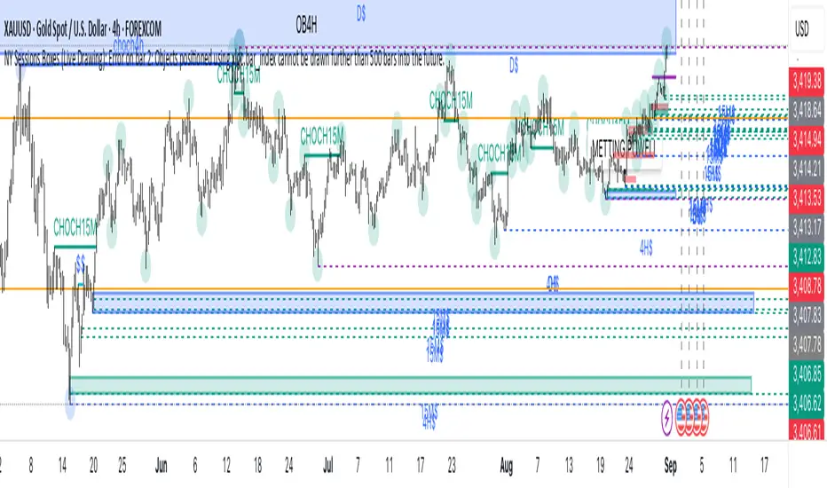
NY Sessions Boxes (Live Drawing)//@version=5
indicator("NY Sessions Boxes (Live Drawing)", overlay=true)
ny_tz = "America/New_York"
t = time(timeframe.period, ny_tz)
hour_ny = hour(t)
minute_ny = minute(t)
// سشن ۱: 02:00 – 05:00
session1_active = (hour_ny >= 2 and hour_ny < 5)
session1_start = (hour_ny == 2 and minute_ny == 0)
// سشن ۲: 09:30 – 11:00
session2_active = ((hour_ny == 9 and minute_ny >= 30) or (hour_ny > 9 and hour_ny < 11))
session2_start = (hour_ny == 9 and minute_ny == 30)
var box box1 = na
var float hi1 = na
var float lo1 = na
if session1_start
hi1 := high
lo1 := low
box1 := box.new(left = time, right = time, top = high, bottom = low, bgcolor=color.new(color.blue, 85), border_color=color.blue)
if session1_active and not na(box1)
hi1 := math.max(hi1, high)
lo1 := math.min(lo1, low)
box.set_right(box1, time)
box.set_top(box1, hi1)
box.set_bottom(box1, lo1)
if not session1_active and not na(box1)
box1 := na
hi1 := na
lo1 := na
var box box2 = na
var float hi2 = na
var float lo2 = na
if session2_start
hi2 := high
lo2 := low
box2 := box.new(left = time, right = time, top = high, bottom = low, bgcolor=color.new(color.purple, 85), border_color=color.purple)
if session2_active and not na(box2)
hi2 := math.max(hi2, high)
lo2 := math.min(lo2, low)
box.set_right(box2, time)
box.set_top(box2, hi2)
box.set_bottom(box2, lo2)
if not session2_active and not na(box2)
box2 := na
hi2 := na
lo2 := na
Median Deviation Suite [InvestorUnknown]The Median Deviation Suite uses a median-based baseline derived from a Double Exponential Moving Average (DEMA) and layers multiple deviation measures around it. By comparing price to these deviation-based ranges, it attempts to identify trends and potential turning points in the market. The indicator also incorporates several deviation types—Average Absolute Deviation (AAD), Median Absolute Deviation (MAD), Standard Deviation (STDEV), and Average True Range (ATR)—allowing traders to visualize different forms of volatility and dispersion. Users should calibrate the settings to suit their specific trading approach, as the default values are not optimized.
Core Components
Median of a DEMA:
The foundation of the indicator is a Median applied to the 7-day DEMA (Double Exponential Moving Average). DEMA aims to reduce lag compared to simple or exponential moving averages. By then taking a median over median_len periods of the DEMA values, the indicator creates a robust and stable central tendency line.
float dema = ta.dema(src, 7)
float median = ta.median(dema, median_len)
Multiple Deviation Measures:
Around this median, the indicator calculates several measures of dispersion:
ATR (Average True Range): A popular volatility measure.
STDEV (Standard Deviation): Measures the spread of price data from its mean.
MAD (Median Absolute Deviation): A robust measure of variability less influenced by outliers.
AAD (Average Absolute Deviation): Similar to MAD, but uses the mean absolute deviation instead of median.
Average of Deviations (avg_dev): The average of the above four measures (ATR, STDEV, MAD, AAD), providing a combined sense of volatility.
Each measure is multiplied by a user-defined multiplier (dev_mul) to scale the width of the bands.
aad = f_aad(src, dev_len, median) * dev_mul
mad = f_mad(src, dev_len, median) * dev_mul
stdev = ta.stdev(src, dev_len) * dev_mul
atr = ta.atr(dev_len) * dev_mul
avg_dev = math.avg(aad, mad, stdev, atr)
Deviation-Based Bands:
The indicator creates multiple upper and lower lines based on each deviation type. For example, using MAD:
float mad_p = median + mad // already multiplied by dev_mul
float mad_m = median - mad
Similar calculations are done for AAD, STDEV, ATR, and the average of these deviations. The indicator then determines the overall upper and lower boundaries by combining these lines:
float upper = f_max4(aad_p, mad_p, stdev_p, atr_p)
float lower = f_min4(aad_m, mad_m, stdev_m, atr_m)
float upper2 = f_min4(aad_p, mad_p, stdev_p, atr_p)
float lower2 = f_max4(aad_m, mad_m, stdev_m, atr_m)
This creates a layered structure of volatility envelopes. Traders can observe which layers price interacts with to gauge trend strength.
Determining Trend
The indicator generates trend signals by assessing where price stands relative to these deviation-based lines. It assigns a trend score by summing individual signals from each deviation measure. For instance, if price crosses above the MAD-based upper line, it contributes a bullish point; crossing below an ATR-based lower line contributes a bearish point.
When the aggregated trend score crosses above zero, it suggests a shift towards a bullish environment; crossing below zero indicates a bearish bias.
// Define Trend scores
var int aad_t = 0
if ta.crossover(src, aad_p)
aad_t := 1
if ta.crossunder(src, aad_m)
aad_t := -1
var int mad_t = 0
if ta.crossover(src, mad_p)
mad_t := 1
if ta.crossunder(src, mad_m)
mad_t := -1
var int stdev_t = 0
if ta.crossover(src, stdev_p)
stdev_t := 1
if ta.crossunder(src, stdev_m)
stdev_t := -1
var int atr_t = 0
if ta.crossover(src, atr_p)
atr_t := 1
if ta.crossunder(src, atr_m)
atr_t := -1
var int adev_t = 0
if ta.crossover(src, adev_p)
adev_t := 1
if ta.crossunder(src, adev_m)
adev_t := -1
int upper_t = src > upper ? 3 : 0
int lower_t = src < lower ? 0 : -3
int upper2_t = src > upper2 ? 1 : 0
int lower2_t = src < lower2 ? 0 : -1
float trend = aad_t + mad_t + stdev_t + atr_t + adev_t + upper_t + lower_t + upper2_t + lower2_t
var float sig = 0
if ta.crossover(trend, 0)
sig := 1
else if ta.crossunder(trend, 0)
sig := -1
Practical Usage and Calibration
Default settings are not optimized: The given parameters serve as a starting point for demonstration. Users should adjust:
median_len: Affects how smooth and lagging the median of the DEMA is.
dev_len and dev_mul: Influence the sensitivity of the deviation measures. Larger multipliers widen the bands, potentially reducing false signals but introducing more lag. Smaller multipliers tighten the bands, producing quicker signals but potentially more whipsaws.
This flexibility allows the trader to tailor the indicator for various markets (stocks, forex, crypto) and time frames.
Backtesting and Performance Metrics
The code integrates with a backtesting library that allows traders to:
Evaluate the strategy historically
Compare the indicator’s signals with a simple buy-and-hold approach
Generate performance metrics (e.g., mean returns, Sharpe Ratio, Sortino Ratio) to assess historical effectiveness.
Disclaimer
No guaranteed results: Historical performance does not guarantee future outcomes. Market conditions can vary widely.
User responsibility: Traders should combine this indicator with other forms of analysis, appropriate risk management, and careful calibration of parameters.
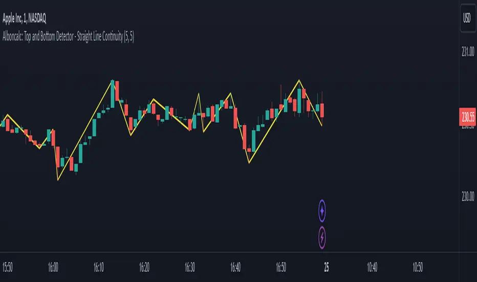
Alboncalc: Top and Bottom Detector - Straight Line ContinuityDescription:
The "Alboncalc: Top and Bottom Detector - Straight Line Continuity" is an innovative indicator for identifying key price reversal points (tops and bottoms) with precision. Unlike traditional indicators that focus on abstract data representations like oscillators or momentum-based lines, this indicator directly overlays the price chart. It draws a continuous line connecting highs and lows (tops and bottoms), providing traders with a clear and immediate visual representation of market swings. The lines automatically adjust in real-time, maintaining a straight path during trend continuations and only shifting when a trend reversal is detected.
Originality and Usefulness:
This indicator stands out from other tools available on TradingView due to its unique ability to maintain a continuous line across price swings, preserving accuracy and visual clarity. Most traditional top-and-bottom detectors merely mark points or provide indicators that are disconnected from price action, making it harder for traders to spot patterns. This script takes a different approach by drawing lines directly on the price chart, offering greater precision and better trend visualization. This innovation is particularly useful for traders who rely on visual cues and price action analysis to make decisions. It simplifies the process of identifying reversal points and trends without needing to rely on lagging indicators.
How It Works:
This indicator detects tops and bottoms based on user-defined periods. When the highest point in a given period is detected, it marks it as a top, and similarly, when the lowest point is detected, it marks it as a bottom. As the price moves, the indicator adjusts the lines to connect consecutive tops and bottoms. If the trend continues in the same direction (e.g., an uptrend), the line remains straight and extends. If a reversal is detected, a new line is drawn to connect the previous bottom (or top) to the new reversal point, providing an accurate visual representation of market trends.
How to Use:
1. Load the Indicator: Add the "Alboncalc: Top and Bottom Detector - Straight Line Continuity" to your chart from the TradingView script library.
2. Customize Settings: Adjust the "Top Period" and "Bottom Period" inputs to fine-tune the sensitivity of top and bottom detection based on your preferred timeframe.
3. Observe Price Action: As the price moves, the indicator will draw lines directly over the price chart, connecting tops and bottoms.
4. Interpret the Lines: Use the continuous lines to identify ongoing trends and potential reversal points. The line remains straight during trend continuation, indicating sustained movement in one direction. A new line signifies a reversal in the trend.
This tool is ideal for traders using trend-following strategies, breakout detection, or those who prefer clean, visual price action analysis (Only Tops and Bottons).
Underlying Concepts:
The core of this indicator is based on the highest high and lowest low concept, which is common in technical analysis. The logic is simple:
- A top is detected when the price reaches a high point compared to a user-defined number of prior candles (i.e., the `top_period`).
- A bottom is detected when the price hits a low point compared to the prior candles (i.e., the `bottom_period`).
When the price continues in the same trend, the line is extended without a break. This behavior ensures that trends are represented in a clear and consistent manner, which helps traders better identify trend continuations and reversals.
Code Breakdown:
```pinescript
//@version=5
indicator("Top and Bottom Detector - Straight Line Continuity", overlay=true)
```
- This initializes the indicator and specifies that it will overlay directly on the price chart.
```pinescript
var int top_period = input.int(5, title="Top Period", minval=1)
var int bottom_period = input.int(5, title="Bottom Period", minval=1)
```
- These inputs allow the user to customize the number of candles used to identify tops and bottoms. A higher period results in fewer but more significant top/bottom detections, while a lower period increases sensitivity.
```pinescript
isTop = ta.highest(top_period) == high
isBottom = ta.lowest(bottom_period) == low
```
- These lines check if the current candle has the highest high or the lowest low in the defined period. If true, the current price is either a top or a bottom.
```pinescript
var line currentLine = na
var float last_price = na
var int last_index = na
var bool isUpTrend = na
```
- These variables store the current line being drawn (`currentLine`), the last detected price (`last_price`), and the direction of the trend (`isUpTrend`). `last_index` tracks where the last top or bottom was detected.
```pinescript
if (isTop or isBottom)
if (not na(last_price))
if ((isTop and isUpTrend) or (isBottom and not isUpTrend))
line.set_xy2(currentLine, bar_index, (isTop ? high : low))
else
currentLine := line.new(x1=last_index, y1=last_price, x2=bar_index, y2=(isTop ? high : low), color=color.yellow, width=2)
last_price := (isTop ? high : low)
last_index := bar_index
isUpTrend := isTop
```
- The `if` block handles the logic of drawing the line. If a top or bottom is detected, and the trend continues (either an uptrend for tops or a downtrend for bottoms), the current line is extended using `line.set_xy2`. If a reversal is detected, a new line is drawn using `line.new`.
- The `last_price` and `last_index` variables are updated after each detection, and the `isUpTrend` flag is set based on whether a top or bottom was found.
Conclusion:
This indicator offers a more precise and visually intuitive way of identifying tops and bottoms directly on the price chart, making it an essential tool for traders focused on price action. Its ability to draw continuous lines through ongoing trends and adjust only upon a reversal makes it superior in terms of visual clarity compared to most conventional indicators.
analytics_tablesLibrary "analytics_tables"
📝 Description
This library provides the implementation of several performance-related statistics and metrics, presented in the form of tables.
The metrics shown in the afforementioned tables where developed during the past years of my in-depth analalysis of various strategies in an atempt to reason about the performance of each strategy.
The visualization and some statistics where inspired by the existing implementations of the "Seasonality" script, and the performance matrix implementations of @QuantNomad and @ZenAndTheArtOfTrading scripts.
While this library is meant to be used by my strategy framework "Template Trailing Strategy (Backtester)" script, I wrapped it in a library hoping this can be usefull for other community strategy scripts that will be released in the future.
🤔 How to Guide
To use the functionality this library provides in your script you have to import it first!
Copy the import statement of the latest release by pressing the copy button below and then paste it into your script. Give a short name to this library so you can refer to it later on. The import statement should look like this:
import jason5480/analytics_tables/1 as ant
There are three types of tables provided by this library in the initial release. The stats table the metrics table and the seasonality table.
Each one shows different kinds of performance statistics.
The table UDT shall be initialized once using the `init()` method.
They can be updated using the `update()` method where the updated data UDT object shall be passed.
The data UDT can also initialized and get updated on demend depending on the use case
A code example for the StatsTable is the following:
var ant.StatsData statsData = ant.StatsData.new()
statsData.update(SideStats.new(), SideStats.new(), 0)
if (barstate.islastconfirmedhistory or (barstate.isrealtime and barstate.isconfirmed))
var statsTable = ant.StatsTable.new().init(ant.getTablePos('TOP', 'RIGHT'))
statsTable.update(statsData)
A code example for the MetricsTable is the following:
var ant.StatsData statsData = ant.StatsData.new()
statsData.update(ant.SideStats.new(), ant.SideStats.new(), 0)
if (barstate.islastconfirmedhistory or (barstate.isrealtime and barstate.isconfirmed))
var metricsTable = ant.MetricsTable.new().init(ant.getTablePos('BOTTOM', 'RIGHT'))
metricsTable.update(statsData, 10)
A code example for the SeasonalityTable is the following:
var ant.SeasonalData seasonalData = ant.SeasonalData.new().init(Seasonality.monthOfYear)
seasonalData.update()
if (barstate.islastconfirmedhistory or (barstate.isrealtime and barstate.isconfirmed))
var seasonalTable = ant.SeasonalTable.new().init(seasonalData, ant.getTablePos('BOTTOM', 'LEFT'))
seasonalTable.update(seasonalData)
🏋️♂️ Please refer to the "EXAMPLE" regions of the script for more advanced and up to date code examples!
Special thanks to @Mrcrbw for the proposal to develop this library and @DCNeu for the constructive feedback 🏆.
getTablePos(ypos, xpos)
Get table position compatible string
Parameters:
ypos (simple string) : The position on y axise
xpos (simple string) : The position on x axise
Returns: The position to be passed to the table
method init(this, pos, height, width, positiveTxtColor, negativeTxtColor, neutralTxtColor, positiveBgColor, negativeBgColor, neutralBgColor)
Initialize the stats table object with the given colors in the given position
Namespace types: StatsTable
Parameters:
this (StatsTable) : The stats table object
pos (simple string) : The table position string
height (simple float) : The height of the table as a percentage of the charts height. By default, 0 auto-adjusts the height based on the text inside the cells
width (simple float) : The width of the table as a percentage of the charts height. By default, 0 auto-adjusts the width based on the text inside the cells
positiveTxtColor (simple color) : The text color when positive
negativeTxtColor (simple color) : The text color when negative
neutralTxtColor (simple color) : The text color when neutral
positiveBgColor (simple color) : The background color with transparency when positive
negativeBgColor (simple color) : The background color with transparency when negative
neutralBgColor (simple color) : The background color with transparency when neutral
method init(this, pos, height, width, neutralBgColor)
Initialize the metrics table object with the given colors in the given position
Namespace types: MetricsTable
Parameters:
this (MetricsTable) : The metrics table object
pos (simple string) : The table position string
height (simple float) : The height of the table as a percentage of the charts height. By default, 0 auto-adjusts the height based on the text inside the cells
width (simple float) : The width of the table as a percentage of the charts width. By default, 0 auto-adjusts the width based on the text inside the cells
neutralBgColor (simple color) : The background color with transparency when neutral
method init(this, seas)
Initialize the seasonal data
Namespace types: SeasonalData
Parameters:
this (SeasonalData) : The seasonal data object
seas (simple Seasonality) : The seasonality of the matrix data
method init(this, data, pos, maxNumOfYears, height, width, extended, neutralTxtColor, neutralBgColor)
Initialize the seasonal table object with the given colors in the given position
Namespace types: SeasonalTable
Parameters:
this (SeasonalTable) : The seasonal table object
data (SeasonalData) : The seasonality data of the table
pos (simple string) : The table position string
maxNumOfYears (simple int) : The maximum number of years that fit into the table
height (simple float) : The height of the table as a percentage of the charts height. By default, 0 auto-adjusts the height based on the text inside the cells
width (simple float) : The width of the table as a percentage of the charts width. By default, 0 auto-adjusts the width based on the text inside the cells
extended (simple bool) : The seasonal table with extended columns for performance
neutralTxtColor (simple color) : The text color when neutral
neutralBgColor (simple color) : The background color with transparency when neutral
method update(this, wins, losses, numOfInconclusiveExits)
Update the strategy info data of the strategy
Namespace types: StatsData
Parameters:
this (StatsData) : The strategy statistics object
wins (SideStats)
losses (SideStats)
numOfInconclusiveExits (int) : The number of inconclusive trades
method update(this, stats, positiveTxtColor, negativeTxtColor, negativeBgColor, neutralBgColor)
Update the stats table object with the given data
Namespace types: StatsTable
Parameters:
this (StatsTable) : The stats table object
stats (StatsData) : The stats data to update the table
positiveTxtColor (simple color) : The text color when positive
negativeTxtColor (simple color) : The text color when negative
negativeBgColor (simple color) : The background color with transparency when negative
neutralBgColor (simple color) : The background color with transparency when neutral
method update(this, stats, buyAndHoldPerc, positiveTxtColor, negativeTxtColor, positiveBgColor, negativeBgColor)
Update the metrics table object with the given data
Namespace types: MetricsTable
Parameters:
this (MetricsTable) : The metrics table object
stats (StatsData) : The stats data to update the table
buyAndHoldPerc (float) : The buy and hold percetage
positiveTxtColor (simple color) : The text color when positive
negativeTxtColor (simple color) : The text color when negative
positiveBgColor (simple color) : The background color with transparency when positive
negativeBgColor (simple color) : The background color with transparency when negative
method update(this)
Update the seasonal data based on the season and eon timeframe
Namespace types: SeasonalData
Parameters:
this (SeasonalData) : The seasonal data object
method update(this, data, positiveTxtColor, negativeTxtColor, neutralTxtColor, positiveBgColor, negativeBgColor, neutralBgColor, timeBgColor)
Update the seasonal table object with the given data
Namespace types: SeasonalTable
Parameters:
this (SeasonalTable) : The seasonal table object
data (SeasonalData) : The seasonal cell data to update the table
positiveTxtColor (simple color) : The text color when positive
negativeTxtColor (simple color) : The text color when negative
neutralTxtColor (simple color) : The text color when neutral
positiveBgColor (simple color) : The background color with transparency when positive
negativeBgColor (simple color) : The background color with transparency when negative
neutralBgColor (simple color) : The background color with transparency when neutral
timeBgColor (simple color) : The background color of the time gradient
SideStats
Object that represents the strategy statistics data of one side win or lose
Fields:
numOf (series int)
sumFreeProfit (series float)
freeProfitStDev (series float)
sumProfit (series float)
profitStDev (series float)
sumGain (series float)
gainStDev (series float)
avgQuantityPerc (series float)
avgCapitalRiskPerc (series float)
avgTPExecutedCount (series float)
avgRiskRewardRatio (series float)
maxStreak (series int)
StatsTable
Object that represents the stats table
Fields:
table (series table) : The actual table
rows (series int) : The number of rows of the table
columns (series int) : The number of columns of the table
StatsData
Object that represents the statistics data of the strategy
Fields:
wins (SideStats)
losses (SideStats)
numOfInconclusiveExits (series int)
avgFreeProfitStr (series string)
freeProfitStDevStr (series string)
lossFreeProfitStDevStr (series string)
avgProfitStr (series string)
profitStDevStr (series string)
lossProfitStDevStr (series string)
avgQuantityStr (series string)
MetricsTable
Object that represents the metrics table
Fields:
table (series table) : The actual table
rows (series int) : The number of rows of the table
columns (series int) : The number of columns of the table
SeasonalData
Object that represents the seasonal table dynamic data
Fields:
seasonality (series Seasonality)
eonToMatrixRow (map)
numOfEons (series int)
mostRecentMatrixRow (series int)
balances (matrix)
returnPercs (matrix)
maxDDs (matrix)
eonReturnPercs (array)
eonCAGRs (array)
eonMaxDDs (array)
SeasonalTable
Object that represents the seasonal table
Fields:
table (series table) : The actual table
headRows (series int) : The number of head rows of the table
headColumns (series int) : The number of head columns of the table
eonRows (series int) : The number of eon rows of the table
seasonColumns (series int) : The number of season columns of the table
statsRows (series int)
statsColumns (series int) : The number of stats columns of the table
rows (series int) : The number of rows of the table
columns (series int) : The number of columns of the table
extended (series bool) : Whether the table has additional performance statistics

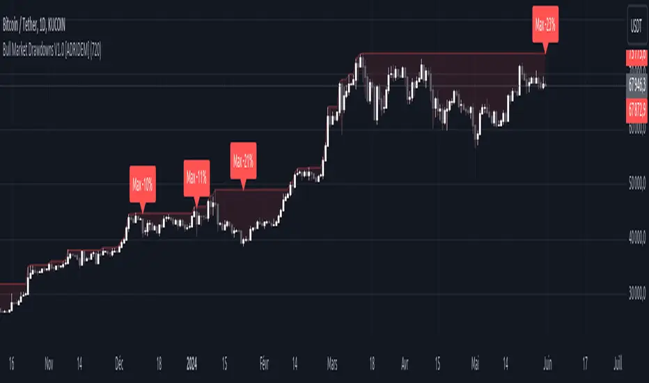
Bull Market Drawdowns V1.0 [ADRIDEM]Bull Market Drawdowns V1.0
Overview
The Bull Market Drawdowns V1.0 script is designed to help visualize and analyze drawdowns during a bull market. This script calculates the highest high price from a specified start date, identifies drawdown periods, and plots the drawdown areas on the chart. It also highlights the maximum drawdowns and marks the start of the bull market, providing a clear visual representation of market performance and potential risk periods.
Unique Features of the New Script
Default Timeframe Configuration: Allows users to set a default timeframe for analysis, providing flexibility in adapting the script to different trading strategies and market conditions.
Customizable Bull Market Start Date: Users can define the start date of the bull market, ensuring the script calculates drawdowns from a specific point in time that aligns with their analysis.
Drawdown Calculation and Visualization: Calculates drawdowns from the highest high since the bull market start date and plots the drawdown areas on the chart with distinct color fills for easy identification.
Maximum Drawdown Tracking and Labeling: Tracks the maximum drawdown for each period and places labels on the chart to indicate significant drawdowns, helping traders identify and assess periods of higher risk.
Bull Market Start Marker: Marks the start of the bull market on the chart with a label, providing a clear reference point for the beginning of the analysis period.
Originality and Usefulness
This script provides a unique and valuable tool by combining drawdown analysis with visual markers and customizable settings. By calculating and plotting drawdowns from a user-defined start date, traders can better understand the performance and risks associated with a bull market. The script’s ability to track and label maximum drawdowns adds further depth to the analysis, making it easier to identify critical periods of market retracement.
Signal Description
The script includes several key visual elements that enhance its usefulness for traders:
Drawdown Area : Plots the upper and lower boundaries of the drawdown area, filling the space between with a semi-transparent color. This helps traders easily identify periods of market retracement.
Maximum Drawdown Labels : Labels are placed on the chart to indicate the maximum drawdown for each period, providing clear markers for significant drawdowns.
Bull Market Start Marker : A label is placed at the start of the bull market, marking the beginning of the analysis period and helping traders contextualize the drawdown data.
These visual elements help quickly assess the extent and impact of drawdowns within a bull market, aiding in risk management and decision-making.
Detailed Description
Input Variables
Default Timeframe (`default_timeframe`) : Defines the timeframe for the analysis. Default is 720 minutes
Bull Market Start Date (`start_date_input`) : The starting date for the bull market analysis. Default is January 1, 2023
Functionality
Highest High Calculation : The script calculates the highest high price on the specified timeframe from the user-defined start date.
```pine
var float highest_high = na
if (time >= start_date)
highest_high := na(highest_high ) ? high : math.max(highest_high , high)
```
Drawdown Calculation : Determines the drawdown starting point and calculates the drawdown percentage from the highest high.
```pine
var float drawdown_start = na
if (time >= start_date)
drawdown_start := na(drawdown_start ) or high >= highest_high ? high : drawdown_start
drawdown = (drawdown_start - low) / drawdown_start * 100
```
Maximum Drawdown Tracking : Tracks the maximum drawdown for each period and places labels above the highest high when a new high is reached.
```pine
var float max_drawdown = na
var int max_drawdown_bar_index = na
if (time >= start_date)
if na(max_drawdown ) or high >= highest_high
if not na(max_drawdown ) and not na(max_drawdown_bar_index) and max_drawdown > 10
label.new(x=max_drawdown_bar_index, y=drawdown_start , text="Max -" + str.tostring(max_drawdown , "#") + "%",
color=color.red, style=label.style_label_down, textcolor=color.white, size=size.normal)
max_drawdown := 0
max_drawdown_bar_index := na
else
if na(max_drawdown ) or drawdown > max_drawdown
max_drawdown := drawdown
max_drawdown_bar_index := bar_index
```
Drawdown Area Plotting : Plots the drawdown area with upper and lower boundaries and fills the area with a semi-transparent color.
```pine
drawdown_area_upper = time >= start_date ? drawdown_start : na
drawdown_area_lower = time >= start_date ? low : na
p1 = plot(drawdown_area_upper, title="Drawdown Area Upper", color=color.rgb(255, 82, 82, 60), linewidth=1)
p2 = plot(drawdown_area_lower, title="Drawdown Area Lower", color=color.rgb(255, 82, 82, 100), linewidth=1)
fill(p1, p2, color=color.new(color.red, 90), title="Drawdown Fill")
```
Current Maximum Drawdown Label : Places a label on the chart to indicate the current maximum drawdown if it exceeds 10%.
```pine
var label current_max_drawdown_label = na
if (not na(max_drawdown) and max_drawdown > 10)
current_max_drawdown_label := label.new(x=bar_index, y=drawdown_start, text="Max -" + str.tostring(max_drawdown, "#") + "%",
color=color.red, style=label.style_label_down, textcolor=color.white, size=size.normal)
if (not na(current_max_drawdown_label))
label.delete(current_max_drawdown_label )
```
Bull Market Start Marker : Places a label at the start of the bull market to mark the beginning of the analysis period.
```pine
var label bull_market_start_label = na
if (time >= start_date and na(bull_market_start_label))
bull_market_start_label := label.new(x=bar_index, y=high, text="Bull Market Start", color=color.blue, style=label.style_label_up, textcolor=color.white, size=size.normal)
```
How to Use
Configuring Inputs : Adjust the default timeframe and start date for the bull market as needed. This allows the script to be tailored to different market conditions and trading strategies.
Interpreting the Indicator : Use the drawdown areas and labels to identify periods of significant market retracement. Pay attention to the maximum drawdown labels to assess the risk during these periods.
Signal Confirmation : Use the bull market start marker to contextualize drawdown data within the overall market trend. The combination of drawdown visualization and maximum drawdown labels helps in making informed trading decisions.
This script provides a detailed view of drawdowns during a bull market, helping traders make more informed decisions by understanding the extent and impact of market retracements. By combining customizable settings with visual markers and drawdown analysis, traders can better align their strategies with the underlying market conditions, thus improving their risk management and decision-making processes.
Max Drawdown Calculating Functions (Optimized)Maximum Drawdown and Maximum Relative Drawdown% calculating functions.
I needed a way to calculate the maxDD% of a serie of datas from an array (the different values of my balance account). I didn't find any builtin pinescript way to do it, so here it is.
There are 2 algorithms to calculate maxDD and relative maxDD%, one non optimized needs n*(n - 1)/2 comparisons for a collection of n datas, the other one only needs n-1 comparisons.
In the example we calculate the maxDDs of the last 10 close values.
There a 2 functions : "maximum_relative_drawdown" and "maximum_dradown" (and "optimized_maximum_relative_drawdown" and "optimized_maximum_drawdown") with names speaking for themselves.
Input : an array of floats of arbitrary size (the values we want the DD of)
Output : an array of 4 values
I added the iteration number just for fun.
Basically my script is the implementation of these 2 algos I found on the net :
var peak = 0;
var n = prices.length
for (var i = 1; i < n; i++){
dif = prices - prices ;
peak = dif < 0 ? i : peak;
maxDrawdown = maxDrawdown > dif ? maxDrawdown : dif;
}
var n = prices.length
for (var i = 0; i < n; i++){
for (var j = i + 1; j < n; j++){
dif = prices - prices ;
maxDrawdown = maxDrawdown > dif ? maxDrawdown : dif;
}
}
Feel free to use it.
@version=4

BE-Indicator Aggregator toolkit█ Overview:
BE-Indicator Aggregator toolkit is a toolkit which is built for those we rely on taking multi-confirmation from different indicators available with the traders. This Toolkit aid's traders in understanding their custom logic for their trade setups and provides the summarized results on how it performed over the past.
█ How It Works:
Load the external indicator plots in the indicator input setting
Provide your custom logic for the trade setup
Set your expected SL & TP values
█ Legends, Definitions & Logic Building Rules:
Building the logic for your trade setup plays a pivotal role in the toolkit, it shall be broken into parts and toolkit aims to understand each of the logical parts of your setup and interpret the outcome as trade accuracy.
Toolkit broadly aims to understand 4 types of inputs in "Condition Builder"
Comments : Line which starts with single quotation ( ' ) shall be ignored by toolkit while understanding the logic.
Note: Blank line space or less than 3 characters are treated equally to comments.
Long Condition: Line which starts with " L- " shall be considered for identifying Long setups.
Short Condition: Line which starts with " S- " shall be considered for identifying Short setups.
Variables: Line which starts with " VAR- " shall be considered as variables. Variables can be one such criteria for Long or short condition.
Building Rules: Define all variables first then specify the condition. The usual declare and assign concept of programming. :p)
Criteria Rules: Criteria are individual logic for your one parent condition. multiple criteria can be present in one condition. Each parameter should be delimited with ' | ' key and each criteria should be delimited with ' , ' (Comma with a space - IMPORTANT!!!)
█ Sample Codes for Conditional Builder:
For Trading Long when Open = Low
For Trading Short when Open = High with a Red candle
'Long Setup <---- Comment
L-O|E|L
' E <- in the above line refers to Equals ' = '
'Short Setup
S-AND:O|E|H, O|G|C
' 2 Criteria for used building one condition. Since, both have to satisfied used "AND:" logic.
Understanding of Operator Legends:
"E" => Refers to Equals
"NE" => Refers to Not Equals
"NEOR" => Logical value is Either Comparing value 1 or Comparing value 2
"NEAND" => Logical value is Comparing value 1 And Comparing value 2
"G" => Logical value Greater than Comparing value 1
"GE" => Logical value Greater than and equal to Comparing value 1
"L" => Logical value Lesser than Comparing value 1
"LE" => Logical value Lesser than and equal to Comparing value 1
"B" => Logical value is Between Comparing value 1 & Comparing value 2
"BE" => Logical value is Between or Equal to Comparing value 1 & Comparing value 2
"OSE" => Logical value is Outside of Comparing value 1 & Comparing value 2
"OSI" => Logical value is Outside or Equal to Comparing value 1 & Comparing value 2
"ERR" => Logical value is 'na'
"NERR" => Logical value is not 'na'
"CO" => Logical value Crossed Over Comparing value 1
"CU" => Logical value Crossed Under Comparing value 1
Understanding of Condition Legends:
AND: -> All criteria's to be satisfied for the condition to be True.
NAND: -> Output of AND condition shall be Inversed for the condition to be True.
OR: -> One of criteria to be satisfied for the condition to be True.
NOR: -> Output of OR condition shall be Inversed for the condition to be True.
ATLEAST:X: -> At-least X no of criteria to be satisfied for the condition to be True.
Note: "X" can be any number
NATLEAST:X: -> Output of ATLEAST condition shall be Inversed for the condition to be True
WASTRUE:X: -> Single criteria WAS TRUE within X bar in past for the condition to be True.
Note: "X" can be any number.
ISTRUE:X: -> Single criteria is TRUE since X bar in past for the condition to be True.
Note: "X" can be any number.
Understanding of Variable Legends:
While Condition Supports 8 Types, Variable supports only 6 Types listed below
AND: -> All criteria's to be satisfied for the Variable to be True.
NAND: -> Output of AND condition shall be Inversed for the Variable to be True.
OR: -> One of criteria to be satisfied for the Variable to be True.
NOR: -> Output of OR condition shall be Inversed for the Variable to be True.
ATLEAST:X: -> At-least X no of criteria to be satisfied for the Variable to be True.
Note: "X" can be any number
NATLEAST:X: -> Output of ATLEAST condition shall be Inversed for the Variable to be True
█ Sample Outputs with Logics:
1. RSI Indicator + Technical Indicator: StopLoss: 2.25 against Reward ratio of 1.75 (3.94 value)
Plots Used in Indicator Settings:
Source 1:- RSI
Source 2:- RSI Based MA
Source 3:- Strong Buy
Source 4:- Strong Sell
Logic Used:
For Long Setup : RSI Should be above RSI Based MA, RSI has been Rising when compared to 3 candles ago, Technical Indicator signaled for a Strong Buy on the current candle, however in last 6 candles Technical indicator signaled for Strong Sell.
Similarly Inverse for Short Setup.
L-AND:ES1|GE|ES2, ES1|G|ES1
L-ES3|E|1
L-OR:ES4 |E|1, ES4 |E|1, ES4 |E|1, ES4 |E|1, ES4 |E|1, ES4 |E|1
S-AND:ES1|LE|ES2, ES1|L|ES1
S-ES4|E|1
S-OR:ES3 |E|1, ES3 |E|1, ES3 |E|1, ES3 |E|1, ES3 |E|1, ES3 |E|1
'Note: Last OR condition can also be written by using WASTRUE definition like below
'L-WASTRUE:6:ES4|E|1
'S-WASTRUE:6:ES3|E|1
Output:
2. Volumatic Support / Resistance Levels :
Plots Used in Indicator Settings:
Source 1:- Resistance
Source 2:- Support
Logic Used:
For Long Setup : Long Trade on Liquidity Support.
For Short Setup : Short Trade on Liquidity Resistance.
'Variable Named "ChkLowTradingAbvSupport" is declared to check if last 3 candles is trading above support line of liquidity.
VAR-ChkLowTradingAbvSupport:AND:L|G|ES2, L |G|ES2, L |G|ES2
'Variable Named "ChkCurBarClsdAbv4thBarHigh" is declared to check if current bar closed above the high of previous candle where the Liquidity support is taken (4th Bar).
VAR-ChkCurBarClsdAbv4thBarHigh:OR:C|GE|H , L|G|H
'Combining Condition and Variable to Initiate Long Trade Logic
L-L |LE|ES2
L-AND:ChkLowTradingAbvSupport, ChkCurBarClsdAbv4thBarHigh
VAR-ChkHghTradingBlwRes:AND:H|L|ES1, H |L|ES1, H |L|ES1
VAR-ChkCurBarClsdBlw4thBarLow:OR:C|LE|L , H|L|L
S-H |GE|ES1
S-AND:ChkHghTradingBlwRes, ChkCurBarClsdBlw4thBarLow
Output 1: Day Trading Version
Output 2: Scalper Version
Output 3: Position Version

PIP Algorithm
# **Script Overview (For Non-Coders)**
1. **Purpose**
- The script tries to capture the essential “shape” of price movement by selecting a limited number of “key points” (anchors) from the latest bars.
- After selecting these anchors, it draws straight lines between them, effectively simplifying the price chart into a smaller set of points without losing major swings.
2. **How It Works, Step by Step**
1. We look back a certain number of bars (e.g., 50).
2. We start by drawing a straight line from the **oldest** bar in that range to the **newest** bar—just two points.
3. Next, we find the bar whose price is *farthest away* from that straight line. That becomes a new anchor point.
4. We “snap” (pin) the line to go exactly through that new anchor. Then we re-draw (re-interpolate) the entire line from the first anchor to the last, in segments.
5. We repeat the process (adding more anchors) until we reach the desired number of points. Each time, we choose the biggest gap between our line and the actual price, then re-draw the entire shape.
6. Finally, we connect these anchors on the chart with red lines, visually simplifying the price curve.
3. **Why It’s Useful**
- It highlights the most *important* bends or swings in the price over the chosen window.
- Instead of plotting every single bar, it condenses the information down to the “key turning points.”
4. **Key Takeaway**
- You’ll see a small number of red line segments connecting the **most significant** points in the price data.
- This is especially helpful if you want a simplified view of recent price action without minor fluctuations.
## **Detailed Logic Explanation**
# **Script Breakdown (For Coders)**
//@version=5
indicator(title="PIP Algorithm", overlay=true)
// 1. Inputs
length = input.int(50, title="Lookback Length")
num_points = input.int(5, title="Number of PIP Points (≥ 3)")
// 2. Helper Functions
// ---------------------------------------------------------------------
// reInterpSubrange(...):
// Given two “anchor” indices in `linesArr`, linearly interpolate
// the array values in between so that the subrange forms a straight line
// from linesArr to linesArr .
reInterpSubrange(linesArr, segmentLeft, segmentRight) =>
float leftVal = array.get(linesArr, segmentLeft)
float rightVal = array.get(linesArr, segmentRight)
int segmentLen = segmentRight - segmentLeft
if segmentLen > 1
for i = segmentLeft + 1 to segmentRight - 1
float ratio = (i - segmentLeft) / segmentLen
float interpVal = leftVal + (rightVal - leftVal) * ratio
array.set(linesArr, i, interpVal)
// reInterpolateAllSegments(...):
// For the entire “linesArr,” re-interpolate each subrange between
// consecutive breakpoints in `lineBreaksArr`.
// This ensures the line is globally correct after each new anchor insertion.
reInterpolateAllSegments(linesArr, lineBreaksArr) =>
array.sort(lineBreaksArr, order.asc)
for i = 0 to array.size(lineBreaksArr) - 2
int leftEdge = array.get(lineBreaksArr, i)
int rightEdge = array.get(lineBreaksArr, i + 1)
reInterpSubrange(linesArr, leftEdge, rightEdge)
// getMaxDistanceIndex(...):
// Return the index (bar) that is farthest from the current “linesArr.”
// We skip any indices already in `lineBreaksArr`.
getMaxDistanceIndex(linesArr, closeArr, lineBreaksArr) =>
float maxDist = -1.0
int maxIdx = -1
int sizeData = array.size(linesArr)
for i = 1 to sizeData - 2
bool isBreak = false
for b = 0 to array.size(lineBreaksArr) - 1
if i == array.get(lineBreaksArr, b)
isBreak := true
break
if not isBreak
float dist = math.abs(array.get(linesArr, i) - array.get(closeArr, i))
if dist > maxDist
maxDist := dist
maxIdx := i
maxIdx
// snapAndReinterpolate(...):
// "Snap" a chosen index to its actual close price, then re-interpolate the entire line again.
snapAndReinterpolate(linesArr, closeArr, lineBreaksArr, idxToSnap) =>
if idxToSnap >= 0
float snapVal = array.get(closeArr, idxToSnap)
array.set(linesArr, idxToSnap, snapVal)
reInterpolateAllSegments(linesArr, lineBreaksArr)
// 3. Global Arrays and Flags
// ---------------------------------------------------------------------
// We store final data globally, then use them outside the barstate.islast scope to draw lines.
var float finalCloseData = array.new_float()
var float finalLines = array.new_float()
var int finalLineBreaks = array.new_int()
var bool didCompute = false
var line pipLines = array.new_line()
// 4. Main Logic (Runs Once at the End of the Current Bar)
// ---------------------------------------------------------------------
if barstate.islast
// A) Prepare closeData in forward order (index 0 = oldest bar, index length-1 = newest)
float closeData = array.new_float()
for i = 0 to length - 1
array.push(closeData, close )
// B) Initialize linesArr with a simple linear interpolation from the first to the last point
float linesArr = array.new_float()
float firstClose = array.get(closeData, 0)
float lastClose = array.get(closeData, length - 1)
for i = 0 to length - 1
float ratio = (length > 1) ? (i / float(length - 1)) : 0.0
float val = firstClose + (lastClose - firstClose) * ratio
array.push(linesArr, val)
// C) Initialize lineBreaks with two anchors: 0 (oldest) and length-1 (newest)
int lineBreaks = array.new_int()
array.push(lineBreaks, 0)
array.push(lineBreaks, length - 1)
// D) Iteratively insert new breakpoints, always re-interpolating globally
int iterationsNeeded = math.max(num_points - 2, 0)
for _iteration = 1 to iterationsNeeded
// 1) Re-interpolate entire shape, so it's globally up to date
reInterpolateAllSegments(linesArr, lineBreaks)
// 2) Find the bar with the largest vertical distance to this line
int maxDistIdx = getMaxDistanceIndex(linesArr, closeData, lineBreaks)
if maxDistIdx == -1
break
// 3) Insert that bar index into lineBreaks and snap it
array.push(lineBreaks, maxDistIdx)
array.sort(lineBreaks, order.asc)
snapAndReinterpolate(linesArr, closeData, lineBreaks, maxDistIdx)
// E) Save results into global arrays for line drawing outside barstate.islast
array.clear(finalCloseData)
array.clear(finalLines)
array.clear(finalLineBreaks)
for i = 0 to array.size(closeData) - 1
array.push(finalCloseData, array.get(closeData, i))
array.push(finalLines, array.get(linesArr, i))
for b = 0 to array.size(lineBreaks) - 1
array.push(finalLineBreaks, array.get(lineBreaks, b))
didCompute := true
// 5. Drawing the Lines in Global Scope
// ---------------------------------------------------------------------
// We cannot create lines inside barstate.islast, so we do it outside.
array.clear(pipLines)
if didCompute
// Connect each pair of anchors with red lines
if array.size(finalLineBreaks) > 1
for i = 0 to array.size(finalLineBreaks) - 2
int idxLeft = array.get(finalLineBreaks, i)
int idxRight = array.get(finalLineBreaks, i + 1)
float x1 = bar_index - (length - 1) + idxLeft
float x2 = bar_index - (length - 1) + idxRight
float y1 = array.get(finalCloseData, idxLeft)
float y2 = array.get(finalCloseData, idxRight)
line ln = line.new(x1, y1, x2, y2, extend=extend.none)
line.set_color(ln, color.red)
line.set_width(ln, 2)
array.push(pipLines, ln)
1. **Data Collection**
- We collect the **most recent** `length` bars in `closeData`. Index 0 is the oldest bar in that window, index `length-1` is the newest bar.
2. **Initial Straight Line**
- We create an array called `linesArr` that starts as a simple linear interpolation from `closeData ` (the oldest bar’s close) to `closeData ` (the newest bar’s close).
3. **Line Breaks**
- We store “anchor points” in `lineBreaks`, initially ` `. These are the start and end of our segment.
4. **Global Re-Interpolation**
- Each time we want to add a new anchor, we **re-draw** (linear interpolation) for *every* subrange ` [lineBreaks , lineBreaks ]`, ensuring we have a globally consistent line.
- This avoids the “local subrange only” approach, which can cause clustering near existing anchors.
5. **Finding the Largest Distance**
- After re-drawing, we compute the vertical distance for each bar `i` that isn’t already a line break. The bar with the biggest distance from the line is chosen as the next anchor (`maxDistIdx`).
6. **Snapping and Re-Interpolate**
- We “snap” that bar’s line value to the actual close, i.e. `linesArr = closeData `. Then we globally re-draw all segments again.
7. **Repeat**
- We repeat these insertions until we have the desired number of points (`num_points`).
8. **Drawing**
- Finally, we connect each consecutive pair of anchor points (`lineBreaks`) with a `line.new(...)` call, coloring them red.
- We offset the line’s `x` coordinate so that the anchor at index 0 lines up with `bar_index - (length - 1)`, and the anchor at index `length-1` lines up with `bar_index` (the current bar).
**Result**:
You get a simplified representation of the price with a small set of line segments capturing the largest “jumps” or swings. By re-drawing the entire line after each insertion, the anchors tend to distribute more *evenly* across the data, mitigating the issue where anchors bunch up near each other.
Enjoy experimenting with different `length` and `num_points` to see how the simplified lines change!
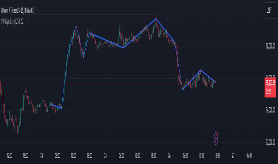
Prometheus StochasticThe Stochastic indicator is a popular indicator developed in the 1950s. It is designed to identify overbought and oversold scenarios on different assets. A value above 80 is considered overbought and a value below 20 is considered oversold.
The formula is as follows:
%k = ((Close - Low_i) / (High_i / Low_i)) * 100
Low_i and High_i represent the lowest low and highest high of the selected period.
The Prometheus version takes a slightly different approach:
%k = ((High - Lowest_Close_i) / (High_i / Low_i)) * 100
Using the Current High minus the Lowest Close provides us with a more robust range that can be slightly more sensitive to moves and provide a different perspective.
Code:
stoch_func(src_close, src_high, src_low, length) =>
100 * (src_high - ta.lowest(src_close, length)) / (ta.highest(src_high, length) - ta.lowest(src_low, length))
This is the function that returns our Stochastic indicator.
What period do we use for the calculation? Let Prometheus handle that, we utilize a Sum of Squared Error calculation to find what lookback values can be most useful for a trader. How we do it is we calculate a Simple Moving Average or SMA and the indicator using a lot of different bars back values. Then if there is an event, characterized by the indicator crossing above 80 or below 20, we subtract the close by the SMA and square it. If there is no event we return a big value, we want the error to be as small as possible. Because we loop over every value for bars back, we get the value with the smallest error. We also do this for the smoothing values.
// Function to calculate SSE for a given combination of N, K, and D
sse_calc(_N, _K, _D) =>
SMA = ta.sma(close, _N)
sf = stoch_func(close, high, low, _N)
k = ta.sma(sf, _K)
d = ta.sma(k, _D)
var float error = na
if ta.crossover(d, 80) or ta.crossunder(d, 20)
error := math.pow(close - SMA, 2)
else
error := 999999999999999999999999999999999999999
error
var int best_N = na
var int best_K = na
var int best_D = na
var float min_SSE = na
// Loop through all combinations of N, K, and D
for N in N_range
for K in K_range
for D in D_range
sse = sse_calc(N, K, D)
if (na(min_SSE) or sse < min_SSE)
min_SSE := sse
best_N := N
best_K := K
best_D := D
int N_opt = na
int K_opt = na
int D_opt = na
if c_lkb_bool == false
N_opt := best_N
K_opt := best_K
D_opt := best_D
This is the section where the best lookback values are calculated.
We provide the option to use this self optimizer or to use your own lookback values.
Here is an example on the daily AMEX:SPY chart. The top Stochastic is the value with the SSE calculation, the bottom is with a fixed 14, 1, 3 input values. We see in the candles with boxes where some potential differences and trades may be.
This is another comparison of the SSE functionality and the fixed lookbacks on the NYSE:PLTR 1 day chart.
Differences may be more apparent on lower time frame charts.
We encourage traders to not follow indicators blindly, none are 100% accurate. SSE does not guarantee that the values generated will be the best for a given moment in time. Please comment on any desired updates, all criticism is welcome!
Adaptive MFT Extremum Pivots [Elysian_Mind]Adaptive MFT Extremum Pivots
Overview:
The Adaptive MFT Extremum Pivots indicator, developed by Elysian_Mind, is a powerful Pine Script tool that dynamically displays key market levels, including Monthly Highs/Lows, Weekly Extremums, Pivot Points, and dynamic Resistances/Supports. The term "dynamic" emphasizes the adaptive nature of the calculated levels, ensuring they reflect real-time market conditions. I thank Zandalin for the excellent table design.
---
Chart Explanation:
The table, a visual output of the script, is conveniently positioned in the bottom right corner of the screen, showcasing the indicator's dynamic results. The configuration block, elucidated in the documentation, empowers users to customize the display position. The default placement is at the bottom right, exemplified in the accompanying chart.
The deliberate design ensures that the table does not obscure the candlesticks, with traders commonly situating it outside the candle area. However, the flexibility exists to overlay the table onto the candles. Thanks to transparent cells, the underlying chart remains visible even with the table displayed atop.
In the initial column of the table, users will find labels for the monthly high and low, accompanied by their respective numerical values. The default precision for these values is set at #.###, yet this can be adjusted within the configuration block to suit markets with varying degrees of volatility.
Mirroring this layout, the last column of the table presents the weekly high and low data. This arrangement is part of the upper half of the table. Transitioning to the lower half, users encounter the resistance levels in the first column and the support levels in the last column.
At the center of the table, prominently displayed, is the monthly pivot point. For a comprehensive understanding of the calculations governing these values, users can refer to the documentation. Importantly, users retain the freedom to modify these mathematical calculations, with the table seamlessly updating to reflect any adjustments made.
Noteworthy is the table's persistence; it continues to display reliably even if users choose to customize the mathematical calculations, providing a consistent and adaptable tool for informed decision-making in trading.
This detailed breakdown offers traders a clear guide to interpreting the information presented by the table, ensuring optimal use and understanding of the Adaptive MFT Extremum Pivots indicator.
---
Usage:
Table Layout:
The table is a crucial component of this indicator, providing a structured representation of various market levels. Color-coded cells enhance readability, with blue indicating key levels and a semi-transparent background to maintain chart visibility.
1. Utilizing a Table for Enhanced Visibility:
In presenting this wealth of information, the indicator employs a table format beneath the chart. The use of a table is deliberate and offers several advantages:
2. Structured Organization:
The table organizes the diverse data into a structured format, enhancing clarity and making it easier for traders to locate specific information.
3. Concise Presentation:
A table allows for the concise presentation of multiple data points without cluttering the main chart. Traders can quickly reference key levels without distraction.
4. Dynamic Visibility:
As the market dynamically evolves, the table seamlessly updates in real-time, ensuring that the most relevant information is readily visible without obstructing the candlestick chart.
5. Color Coding for Readability:
Color-coded cells in the table not only add visual appeal but also serve a functional purpose by improving readability. Key levels are easily distinguishable, contributing to efficient analysis.
Data Values:
Numerical values for each level are displayed in their respective cells, with precision defined by the iPrecision configuration parameter.
Configuration:
// User configuration: You can modify this part without code understanding
// Table location configuration
// Position: Table
const string iPosition = position.bottom_right
// Width: Table borders
const int iBorderWidth = 1
// Color configuration
// Color: Borders
const color iBorderColor = color.new(color.white, 75)
// Color: Table background
const color iTableColor = color.new(#2B2A29, 25)
// Color: Title cell background
const color iTitleCellColor = color.new(#171F54, 0)
// Color: Characters
const color iCharColor = color.white
// Color: Data cell background
const color iDataCellColor = color.new(#25456E, 0)
// Precision: Numerical data
const int iPrecision = 3
// End of configuration
The code includes a configuration block where users can customize the following parameters:
Precision of Numerical Table Data (iPrecision):
// Precision: Numerical data
const int iPrecision = 3
This parameter (iPrecision) sets the precision of the numerical values displayed in the table. The default value is 3, displaying numbers in #.### format.
Position of the Table (iPosition):
// Position: Table
const string iPosition = position.bottom_right
This parameter (iPosition) sets the position of the table on the chart. The default is position.bottom_right.
Color preferences
Table borders (iBorderColor):
// Color: Borders
const color iBorderColor = color.new(color.white, 75)
This parameters (iBorderColor) sets the color of the borders everywhere within the window.
Table Background (iTableColor):
// Color: Table background
const color iTableColor = color.new(#2B2A29, 25)
This is the background color of the table. If you've got cells without custom background color, this color will be their background.
Title Cell Background (iTitleCellColor):
// Color: Title cell background
const color iTitleCellColor = color.new(#171F54, 0)
This is the background color the title cells. You can set the background of data cells and text color elsewhere.
Text (iCharColor):
// Color: Characters
const color iCharColor = color.white
This is the color of the text - titles and data - within the table window. If you change any of the background colors, you might want to change this parameter to ensure visibility.
Data Cell Background: (iDataCellColor):
// Color: Data cell background
const color iDataCellColor = color.new(#25456E, 0)
The data cells have a background color to differ from title cells. You can configure this is a different parameter (iDataColor). You might even set the same color for data as for the titles if you will.
---
Mathematical Background:
Monthly and Weekly Extremums:
The indicator calculates the High (H) and Low (L) of the previous month and week, ensuring accurate representation of these key levels.
Standard Monthly Pivot Point:
The standard pivot point is determined based on the previous month's data using the formula:
PivotPoint = (PrevMonthHigh + PrevMonthLow + Close ) / 3
Monthly Pivot Points (R1, R2, R3, S1, S2, S3):
Additional pivot points are calculated for Resistances (R) and Supports (S) using the monthly data:
R1 = 2 * PivotPoint - PrevMonthLow
S1 = 2 * PivotPoint - PrevMonthHigh
R2 = PivotPoint + (PrevMonthHigh - PrevMonthLow)
S2 = PivotPoint - (PrevMonthHigh - PrevMonthLow)
R3 = PrevMonthHigh + 2 * (PivotPoint - PrevMonthLow)
S3 = PrevMonthLow - 2 * (PrevMonthHigh - PivotPoint)
---
Code Explanation and Interpretation:
The table displayed beneath the chart provides the following information:
Monthly Extremums:
(H) High of the previous month
(L) Low of the previous month
// Function to get the high and low of the previous month
getPrevMonthHighLow() =>
var float prevMonthHigh = na
var float prevMonthLow = na
monthChanged = month(time) != month(time )
if (monthChanged)
prevMonthHigh := high
prevMonthLow := low
Weekly Extremums:
(H) High of the previous week
(L) Low of the previous week
// Function to get the high and low of the previous week
getPrevWeekHighLow() =>
var float prevWeekHigh = na
var float prevWeekLow = na
weekChanged = weekofyear(time) != weekofyear(time )
if (weekChanged)
prevWeekHigh := high
prevWeekLow := low
Monthly Pivots:
Pivot: Standard pivot point based on the previous month's data
// Function to calculate the standard pivot point based on the previous month's data
getStandardPivotPoint() =>
= getPrevMonthHighLow()
pivotPoint = (prevMonthHigh + prevMonthLow + close ) / 3
Resistances:
R3, R2, R1: Monthly resistance levels
// Function to calculate additional pivot points based on the monthly data
getMonthlyPivotPoints() =>
= getPrevMonthHighLow()
pivotPoint = (prevMonthHigh + prevMonthLow + close ) / 3
r1 = (2 * pivotPoint) - prevMonthLow
s1 = (2 * pivotPoint) - prevMonthHigh
r2 = pivotPoint + (prevMonthHigh - prevMonthLow)
s2 = pivotPoint - (prevMonthHigh - prevMonthLow)
r3 = prevMonthHigh + 2 * (pivotPoint - prevMonthLow)
s3 = prevMonthLow - 2 * (prevMonthHigh - pivotPoint)
Initializing and Populating the Table:
The myTable variable initializes the table with a blue background, and subsequent table.cell functions populate the table with headers and data.
// Initialize the table with adjusted bgcolor
var myTable = table.new(position = iPosition, columns = 5, rows = 10, bgcolor = color.new(color.blue, 90), border_width = 1, border_color = color.new(color.blue, 70))
Dynamic Data Population:
Data is dynamically populated in the table using the calculated values for Monthly Extremums, Weekly Extremums, Monthly Pivot Points, Resistances, and Supports.
// Add rows dynamically with data
= getPrevMonthHighLow()
= getPrevWeekHighLow()
= getMonthlyPivotPoints()
---
Conclusion:
The Adaptive MFT Extremum Pivots indicator offers traders a detailed and clear representation of critical market levels, empowering them to make informed decisions. However, users should carefully analyze the market and consider their individual risk tolerance before making any trading decisions. The indicator's disclaimer emphasizes that it is not investment advice, and the author and script provider are not responsible for any financial losses incurred.
---
Disclaimer:
This indicator is not investment advice. Trading decisions should be made based on a careful analysis of the market and individual risk tolerance. The author and script provider are not responsible for any financial losses incurred.
Kind regards,
Ely

Console📕 Console Library
🔷 Introduction
This script is an adaptation of the classic JavaScript console script. It provides a simple way to display data in a console-like table format for debugging purposes.
While there are many nice console/logger scripts out there, my personal goal was to achieve inline functionality and visual object (label, lines) logging .
🔷 How to Use
◼ 1. Import the Console library into your script:
import cryptolinx/Console/1
- or -
Instead of the library namespace, you can define a custom namespace as alias.
import cryptolinx/Console/1 as c
◼ 2. Create and init a new `` object.
The `init()` method is used to initialize the console object with default settings. It can be used to customize it.
// When using the `var` keyword in a declaration, the logs will act as ever-forwarding.
// Without `var`, the `console` variable will be redeclared every time `bar` is called.
// var console = Console.terminal.new(log_position=position.bottom_left, prefix = '> ', show_no = true)
- or -
If you has set up an alias before.
var console = c.terminal.new().init()
◼ 3. Logging
// inline ✨
array testArray = array.new(3, .0).log(console)
// basic
console.log(testArray)
// inline ✨
var testLabel = label.new(bar_index, close, 'Label Text').log(console)
// basic
console.log(testLabel)
// It is also possible to use `().` for literals ✨.
int a = 100
testCalc = (5 * 100).log(console) + a.log(console) // SUM: 600
console.
.empty()
.log('SUM' + WS + testCalc.tostring())
◼ 4. Visibility
Finally, we need to call the `show()` method to display the logged messages in the console.
console.show(true) // True by default. Simply turn it on or off
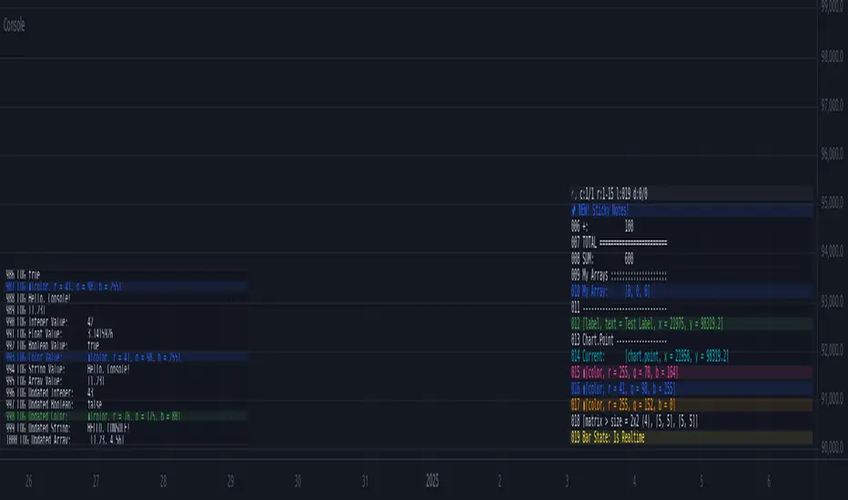
Performance Metrics With Bracketed Rebalacing [BackQuant]Performance Metrics With Bracketed Rebalancing
The Performance Metrics With Bracketed Rebalancing script offers a robust method for assessing portfolio performance, integrating advanced portfolio metrics with different rebalancing strategies. With a focus on adaptability, the script allows traders to monitor and adjust portfolio weights, equity, and other key financial metrics dynamically. This script provides a versatile approach for evaluating different trading strategies, considering factors like risk-adjusted returns, volatility, and the impact of portfolio rebalancing.
Please take the time to read the following:
Key Features and Benefits of Portfolio Methods
Bracketed Rebalancing:
Bracketed Rebalancing is an advanced strategy designed to trigger portfolio adjustments when an asset's weight surpasses a predefined threshold. This approach minimizes overexposure to any single asset while maintaining flexibility in response to market changes. The strategy is particularly beneficial for mitigating risks that arise from significant asset weight fluctuations. The following image illustrates how this method reacts when asset weights cross the threshold:
Daily Rebalancing:
Unlike the bracketed method, Daily Rebalancing adjusts portfolio weights every trading day, ensuring consistent asset allocation. This method aims for a more even distribution of portfolio weights, making it a suitable option for traders who prefer less sensitivity to individual asset volatility. Here's an example of Daily Rebalancing in action:
No Rebalancing:
For traders who prefer a passive approach, the "No Rebalancing" option allows the portfolio to remain static, without any adjustments to asset weights. This method may appeal to long-term investors or those who believe in the inherent stability of their selected assets. Here’s how the portfolio looks when no rebalancing is applied:
Portfolio Weights Visualization:
One of the standout features of this script is the visual representation of portfolio weights. With adjustable settings, users can track the current allocation of assets in real-time, making it easier to analyze shifts and trends. The following image shows the real-time weight distribution across three assets:
Rolling Drawdown Plot:
Managing drawdown risk is a critical aspect of portfolio management. The Rolling Drawdown Plot visually tracks the drawdown over time, helping traders monitor the risk exposure and performance relative to the peak equity levels. This feature is essential for assessing the portfolio's resilience during market downturns:
Daily Portfolio Returns:
Tracking daily returns is crucial for evaluating the short-term performance of the portfolio. The script allows users to plot daily portfolio returns to gain insights into daily profit or loss, helping traders stay updated on their portfolio’s progress:
Performance Metrics
Net Profit (%):
This metric represents the total return on investment as a percentage of the initial capital. A positive net profit indicates that the portfolio has gained value over the evaluation period, while a negative value suggests a loss. It's a fundamental indicator of overall portfolio performance.
Maximum Drawdown (Max DD):
Maximum Drawdown measures the largest peak-to-trough decline in portfolio value during a specified period. It quantifies the most significant loss an investor would have experienced if they had invested at the highest point and sold at the lowest point within the timeframe. A smaller Max DD indicates better risk management and less exposure to significant losses.
Annual Mean Returns (% p/y):
This metric calculates the average annual return of the portfolio over the evaluation period. It provides insight into the portfolio's ability to generate returns on an annual basis, aiding in performance comparison with other investment opportunities.
Annual Standard Deviation of Returns (% p/y):
This measure indicates the volatility of the portfolio's returns on an annual basis. A higher standard deviation signifies greater variability in returns, implying higher risk, while a lower value suggests more stable returns.
Variance:
Variance is the square of the standard deviation and provides a measure of the dispersion of returns. It helps in understanding the degree of risk associated with the portfolio's returns.
Sortino Ratio:
The Sortino Ratio is a variation of the Sharpe Ratio that only considers downside risk, focusing on negative volatility. It is calculated as the difference between the portfolio's return and the minimum acceptable return (MAR), divided by the downside deviation. A higher Sortino Ratio indicates better risk-adjusted performance, emphasizing the importance of avoiding negative returns.
Sharpe Ratio:
The Sharpe Ratio measures the portfolio's excess return per unit of total risk, as represented by standard deviation. It is calculated by subtracting the risk-free rate from the portfolio's return and dividing by the standard deviation of the portfolio's excess return. A higher Sharpe Ratio indicates more favorable risk-adjusted returns.
Omega Ratio:
The Omega Ratio evaluates the probability of achieving returns above a certain threshold relative to the probability of experiencing returns below that threshold. It is calculated by dividing the cumulative probability of positive returns by the cumulative probability of negative returns. An Omega Ratio greater than 1 indicates a higher likelihood of achieving favorable returns.
Gain-to-Pain Ratio:
The Gain-to-Pain Ratio measures the return per unit of risk, focusing on the magnitude of gains relative to the severity of losses. It is calculated by dividing the total gains by the total losses experienced during the evaluation period. A higher ratio suggests a more favorable balance between reward and risk.
www.linkedin.com
Compound Annual Growth Rate (CAGR) (% p/y):
CAGR represents the mean annual growth rate of the portfolio over a specified period, assuming the investment has been compounding over that time. It provides a smoothed annual rate of growth, eliminating the effects of volatility and offering a clearer picture of long-term performance.
Portfolio Alpha (% p/y):
Portfolio Alpha measures the portfolio's performance relative to a benchmark index, adjusting for risk. It is calculated using the Capital Asset Pricing Model (CAPM) and represents the excess return of the portfolio over the expected return based on its beta and the benchmark's performance. A positive alpha indicates outperformance, while a negative alpha suggests underperformance.
Portfolio Beta:
Portfolio Beta assesses the portfolio's sensitivity to market movements, indicating its exposure to systematic risk. A beta greater than 1 suggests the portfolio is more volatile than the market, while a beta less than 1 indicates lower volatility. Beta is used to understand the portfolio's potential for gains or losses in relation to market fluctuations.
Skewness of Returns:
Skewness measures the asymmetry of the return distribution. A positive skew indicates a distribution with a long right tail, suggesting more frequent small losses and fewer large gains. A negative skew indicates a long left tail, implying more frequent small gains and fewer large losses. Understanding skewness helps in assessing the likelihood of extreme outcomes.
Value at Risk (VaR) 95th Percentile:
VaR at the 95th percentile estimates the maximum potential loss over a specified period, given a 95% confidence level. It provides a threshold value such that there is a 95% probability that the portfolio will not experience a loss greater than this amount.
Conditional Value at Risk (CVaR):
CVaR, also known as Expected Shortfall, measures the average loss exceeding the VaR threshold. It provides insight into the tail risk of the portfolio, indicating the expected loss in the worst-case scenarios beyond the VaR level.
These metrics collectively offer a comprehensive view of the portfolio's performance, risk exposure, and efficiency. By analyzing these indicators, investors can make informed decisions, balancing potential returns with acceptable levels of risk.
Conclusion
The Performance Metrics With Bracketed Rebalancing script provides a comprehensive framework for evaluating and optimizing portfolio performance. By integrating advanced metrics, adaptive rebalancing strategies, and visual analytics, it empowers traders to make informed decisions in managing their investment portfolios. However, it's crucial to consider the implications of rebalancing strategies, as academic research indicates that predictable rebalancing can lead to market impact costs. Therefore, adopting flexible and less predictable rebalancing approaches may enhance portfolio performance and reduce associated costs.
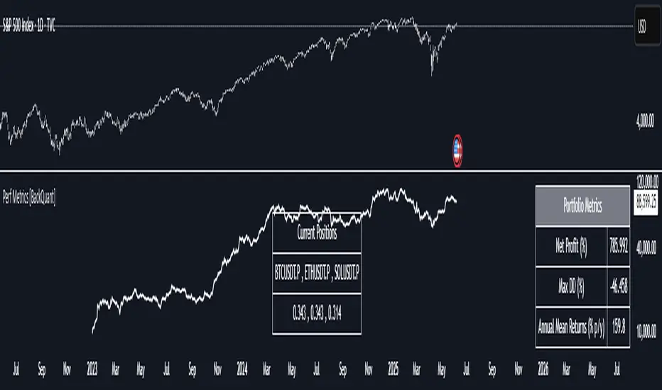
OHLCVRangeXThe OHLCVRange library provides modular range-building utilities for Pine Script v6 based on custom conditions like time, price, volatility, volume, and pattern detection. Each function updates a persistent range (OHLCVRange) passed in from the calling script, based on live streaming candles.
This library is designed to support dynamic windowing over incoming OHLCV bars, with all persistent state handled externally (in the indicator or strategy). The library merely acts as a filter and updater, appending or clearing candles according to custom logic.
📦
export type OHLCVRange
OHLCV.OHLCV candles // Sliding window of candles
The OHLCVRange is a simple container holding an array of OHLCV.OHLCV structures.
This structure should be declared in the indicator using var to ensure persistence across candles.
🧩 Range Updater Functions
Each function follows this pattern:
export updateXxxRange(OHLCVRange r, OHLCV.OHLCV current, ...)
r is the range to update.
current is the latest OHLCV candle (typically from your indicator).
Additional parameters control the behavior of the range filter.
🔁 Function List
1. Fixed Lookback Range
export updateFixedRange(OHLCVRange r, OHLCV.OHLCV current, int barsBack)
Keeps only the last barsBack candles.
Sliding window based purely on number of bars.
2. Session Time Range
export updateSessionRange(OHLCVRange r, OHLCV.OHLCV current, int minuteStart, int minuteEnd)
Keeps candles within the [minuteStart, minuteEnd) intraday session.
Clears the range once out of session bounds.
3. Price Zone Range
export updatePriceZoneRange(OHLCVRange r, OHLCV.OHLCV current, float minP, float maxP)
Retains candles within the vertical price zone .
Clears when a candle exits the zone.
4. Consolidation Range
export updateConsolidationRange(OHLCVRange r, OHLCV.OHLCV current, float thresh)
Stores candles as long as the candle range (high - low) is less than or equal to thresh.
Clears on volatility breakout.
5. Volume Spike Range
export updateVolumeSpikeRange(OHLCVRange r, OHLCV.OHLCV current, float avgVol, float mult, int surround)
Triggers a new range when a volume spike ≥ avgVol * mult occurs.
Adds candles around the spike (total surround * 2 + 1).
Can be used to zoom in around anomalies.
6. Engulfing Pattern Range
export updateEngulfingRange(OHLCVRange r, OHLCV.OHLCV current, int windowAround)
Detects bullish or bearish engulfing candles.
Stores 2 * windowAround + 1 candles centered around the pattern.
Clears if no valid engulfing pattern is found.
7. HTF-Aligned Range
export updateHTFAlignedRange(OHLCVRange r, OHLCV.OHLCV current, OHLCV.OHLCV prevHtf)
Used when aligning lower timeframe candles to higher timeframe bars.
Clears and restarts the range on HTF bar transition (compare prevHtf.bar_index with current).
Requires external management of HTF candle state.
💡 Usage Notes
All OHLCVRange instances should be declared as var in the indicator to preserve state:
var OHLCVRange sessionRange = OHLCVRange.new()
sessionRange := OHLCVRange.updateSessionRange(sessionRange, current, 540, 900)
All OHLCV data should come from the OHLCVData library (v15 or later):
import userId/OHLCVData/15 as OHLCV
OHLCV.OHLCV current = OHLCV.getCurrentChartOHLCV()
This library does not use var internally to enforce clean separation of logic and persistence.
📅 Planned Enhancements
Fib zone ranges: capture candles within custom Fibonacci levels.
Custom event ranges: combine multiple filters (e.g., pattern + volume spike).
Trend-based ranges: windowing based on moving average or trend breaks.

Why EMA Isn't What You Think It IsMany new traders adopt the Exponential Moving Average (EMA) believing it's simply a "better Simple Moving Average (SMA)". This common misconception leads to fundamental misunderstandings about how EMA works and when to use it.
EMA and SMA differ at their core. SMA use a window of finite number of data points, giving equal weight to each data point in the calculation period. This makes SMA a Finite Impulse Response (FIR) filter in signal processing terms. Remember that FIR means that "all that we need is the 'period' number of data points" to calculate the filter value. Anything beyond the given period is not relevant to FIR filters – much like how a security camera with 14-day storage automatically overwrites older footage, making last month's activity completely invisible regardless of how important it might have been.
EMA, however, is an Infinite Impulse Response (IIR) filter. It uses ALL historical data, with each past price having a diminishing - but never zero - influence on the calculated value. This creates an EMA response that extends infinitely into the past—not just for the last N periods. IIR filters cannot be precise if we give them only a 'period' number of data to work on - they will be off-target significantly due to lack of context, like trying to understand Game of Thrones by watching only the final season and wondering why everyone's so upset about that dragon lady going full pyromaniac.
If we only consider a number of data points equal to the EMA's period, we are capturing no more than 86.5% of the total weight of the EMA calculation. Relying on he period window alone (the warm-up period) will provide only 1 - (1 / e^2) weights, which is approximately 1−0.1353 = 0.8647 = 86.5%. That's like claiming you've read a book when you've skipped the first few chapters – technically, you got most of it, but you probably miss some crucial early context.
▶️ What is period in EMA used for?
What does a period parameter really mean for EMA? When we select a 15-period EMA, we're not selecting a window of 15 data points as with an SMA. Instead, we are using that number to calculate a decay factor (α) that determines how quickly older data loses influence in EMA result. Every trader knows EMA calculation: α = 1 / (1+period) – or at least every trader claims to know this while secretly checking the formula when they need it.
Thinking in terms of "period" seriously restricts EMA. The α parameter can be - should be! - any value between 0.0 and 1.0, offering infinite tuning possibilities of the indicator. When we limit ourselves to whole-number periods that we use in FIR indicators, we can only access a small subset of possible IIR calculations – it's like having access to the entire RGB color spectrum with 16.7 million possible colors but stubbornly sticking to the 8 basic crayons in a child's first art set because the coloring book only mentioned those by name.
For example:
Period 10 → alpha = 0.1818
Period 11 → alpha = 0.1667
What about wanting an alpha of 0.17, which might yield superior returns in your strategy that uses EMA? No whole-number period can provide this! Direct α parameterization offers more precision, much like how an analog tuner lets you find the perfect radio frequency while digital presets force you to choose only from predetermined stations, potentially missing the clearest signal sitting right between channels.
Sidenote: the choice of α = 1 / (1+period) is just a convention from 1970s, probably started by J. Welles Wilder, who popularized the use of the 14-day EMA. It was designed to create an approximate equivalence between EMA and SMA over the same number of periods, even thought SMA needs a period window (as it is FIR filter) and EMA doesn't. In reality, the decay factor α in EMA should be allowed any valye between 0.0 and 1.0, not just some discrete values derived from an integer-based period! Algorithmic systems should find the best α decay for EMA directly, allowing the system to fine-tune at will and not through conversion of integer period to float α decay – though this might put a few traditionalist traders into early retirement. Well, to prevent that, most traditionalist implementations of EMA only use period and no alpha at all. Heaven forbid we disturb people who print their charts on paper, draw trendlines with rulers, and insist the market "feels different" since computers do algotrading!
▶️ Calculating EMAs Efficiently
The standard textbook formula for EMA is:
EMA = CurrentPrice × alpha + PreviousEMA × (1 - alpha)
But did you know that a more efficient version exists, once you apply a tiny bit of high school algebra:
EMA = alpha × (CurrentPrice - PreviousEMA) + PreviousEMA
The first one requires three operations: 2 multiplications + 1 addition. The second one also requires three ops: 1 multiplication + 1 addition + 1 subtraction.
That's pathetic, you say? Not worth implementing? In most computational models, multiplications cost much more than additions/subtractions – much like how ordering dessert costs more than asking for a water refill at restaurants.
Relative CPU cost of float operations :
Addition/Subtraction: ~1 cycle
Multiplication: ~5 cycles (depending on precision and architecture)
Now you see the difference? 2 * 5 + 1 = 11 against 5 + 1 + 1 = 7. That is ≈ 36.36% efficiency gain just by swapping formulas around! And making your high school math teacher proud enough to finally put your test on the refrigerator.
▶️ The Warmup Problem: how to start the EMA sequence right
How do we calculate the first EMA value when there's no previous EMA available? Let's see some possible options used throughout the history:
Start with zero : EMA(0) = 0. This creates stupidly large distortion until enough bars pass for the horrible effect to diminish – like starting a trading account with zero balance but backdating a year of missed trades, then watching your balance struggle to climb out of a phantom debt for months.
Start with first price : EMA(0) = first price. This is better than starting with zero, but still causes initial distortion that will be extra-bad if the first price is an outlier – like forming your entire opinion of a stock based solely on its IPO day price, then wondering why your model is tanking for weeks afterward.
Use SMA for warmup : This is the tradition from the pencil-and-paper era of technical analysis – when calculators were luxury items and "algorithmic trading" meant your broker had neat handwriting. We first calculate an SMA over the initial period, then kickstart the EMA with this average value. It's widely used due to tradition, not merit, creating a mathematical Frankenstein that uses an FIR filter (SMA) during the initial period before abruptly switching to an IIR filter (EMA). This methodology is so aesthetically offensive (abrupt kink on the transition from SMA to EMA) that charting platforms hide these early values entirely, pretending EMA simply doesn't exist until the warmup period passes – the technical analysis equivalent of sweeping dust under the rug.
Use WMA for warmup : This one was never popular because it is harder to calculate with a pencil - compared to using simple SMA for warmup. Weighted Moving Average provides a much better approximation of a starting value as its linear descending profile is much closer to the EMA's decay profile.
These methods all share one problem: they produce inaccurate initial values that traders often hide or discard, much like how hedge funds conveniently report awesome performance "since strategy inception" only after their disastrous first quarter has been surgically removed from the track record.
▶️ A Better Way to start EMA: Decaying compensation
Think of it this way: An ideal EMA uses an infinite history of prices, but we only have data starting from a specific point. This creates a problem - our EMA starts with an incorrect assumption that all previous prices were all zero, all close, or all average – like trying to write someone's biography but only having information about their life since last Tuesday.
But there is a better way. It requires more than high school math comprehension and is more computationally intensive, but is mathematically correct and numerically stable. This approach involves compensating calculated EMA values for the "phantom data" that would have existed before our first price point.
Here's how phantom data compensation works:
We start our normal EMA calculation:
EMA_today = EMA_yesterday + α × (Price_today - EMA_yesterday)
But we add a correction factor that adjusts for the missing history:
Correction = 1 at the start
Correction = Correction × (1-α) after each calculation
We then apply this correction:
True_EMA = Raw_EMA / (1-Correction)
This correction factor starts at 1 (full compensation effect) and gets exponentially smaller with each new price bar. After enough data points, the correction becomes so small (i.e., below 0.0000000001) that we can stop applying it as it is no longer relevant.
Let's see how this works in practice:
For the first price bar:
Raw_EMA = 0
Correction = 1
True_EMA = Price (since 0 ÷ (1-1) is undefined, we use the first price)
For the second price bar:
Raw_EMA = α × (Price_2 - 0) + 0 = α × Price_2
Correction = 1 × (1-α) = (1-α)
True_EMA = α × Price_2 ÷ (1-(1-α)) = Price_2
For the third price bar:
Raw_EMA updates using the standard formula
Correction = (1-α) × (1-α) = (1-α)²
True_EMA = Raw_EMA ÷ (1-(1-α)²)
With each new price, the correction factor shrinks exponentially. After about -log₁₀(1e-10)/log₁₀(1-α) bars, the correction becomes negligible, and our EMA calculation matches what we would get if we had infinite historical data.
This approach provides accurate EMA values from the very first calculation. There's no need to use SMA for warmup or discard early values before output converges - EMA is mathematically correct from first value, ready to party without the awkward warmup phase.
Here is Pine Script 6 implementation of EMA that can take alpha parameter directly (or period if desired), returns valid values from the start, is resilient to dirty input values, uses decaying compensator instead of SMA, and uses the least amount of computational cycles possible.
// Enhanced EMA function with proper initialization and efficient calculation
ema(series float source, simple int period=0, simple float alpha=0)=>
// Input validation - one of alpha or period must be provided
if alpha<=0 and period<=0
runtime.error("Alpha or period must be provided")
// Calculate alpha from period if alpha not directly specified
float a = alpha > 0 ? alpha : 2.0 / math.max(period, 1)
// Initialize variables for EMA calculation
var float ema = na // Stores raw EMA value
var float result = na // Stores final corrected EMA
var float e = 1.0 // Decay compensation factor
var bool warmup = true // Flag for warmup phase
if not na(source)
if na(ema)
// First value case - initialize EMA to zero
// (we'll correct this immediately with the compensation)
ema := 0
result := source
else
// Standard EMA calculation (optimized formula)
ema := a * (source - ema) + ema
if warmup
// During warmup phase, apply decay compensation
e *= (1-a) // Update decay factor
float c = 1.0 / (1.0 - e) // Calculate correction multiplier
result := c * ema // Apply correction
// Stop warmup phase when correction becomes negligible
if e <= 1e-10
warmup := false
else
// After warmup, EMA operates without correction
result := ema
result // Return the properly compensated EMA value
▶️ CONCLUSION
EMA isn't just a "better SMA"—it is a fundamentally different tool, like how a submarine differs from a sailboat – both float, but the similarities end there. EMA responds to inputs differently, weighs historical data differently, and requires different initialization techniques.
By understanding these differences, traders can make more informed decisions about when and how to use EMA in trading strategies. And as EMA is embedded in so many other complex and compound indicators and strategies, if system uses tainted and inferior EMA calculatiomn, it is doing a disservice to all derivative indicators too – like building a skyscraper on a foundation of Jell-O.
The next time you add an EMA to your chart, remember: you're not just looking at a "faster moving average." You're using an INFINITE IMPULSE RESPONSE filter that carries the echo of all previous price actions, properly weighted to help make better trading decisions.
EMA done right might significantly improve the quality of all signals, strategies, and trades that rely on EMA somewhere deep in its algorithmic bowels – proving once again that math skills are indeed useful after high school, no matter what your guidance counselor told you.
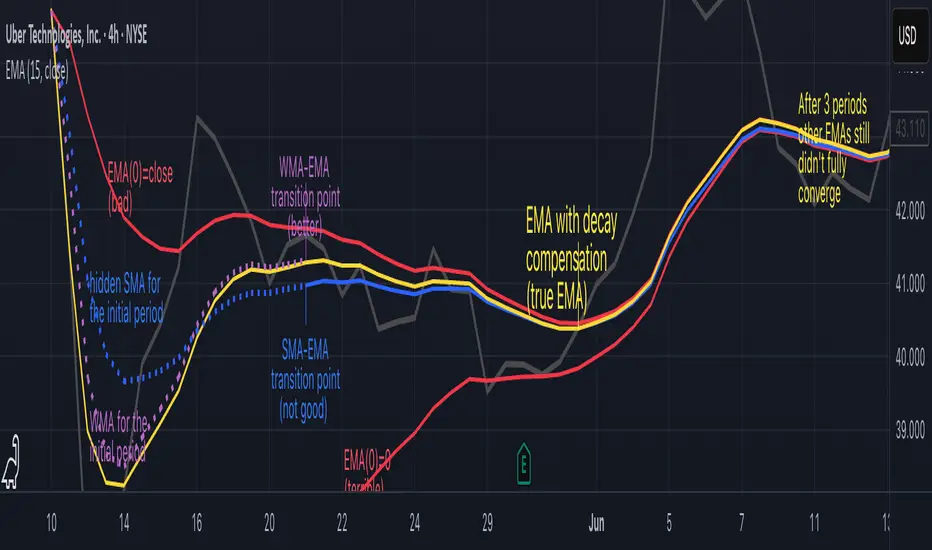
Test OHLCV LibraryThis indicator, "Test OHLCV Library," serves as a practical example of how to use the OHLCVData library to fetch historical candle data from a specific timeframe (like 4H) in a way that is largely impervious to the chart's currently selected time frame.
Here's a breakdown of its purpose and how it addresses request.security limitations:
Indicator Purpose:
The main goal of this indicator is to demonstrate and verify that the OHLCVData library can reliably provide confirmed historical OHLCV data for a user-specified timeframe (e.g., 4H), and that a collection of these data points (the last 10 completed candles) remains consistent even when the user switches the chart's time frame (e.g., from 5-second to Daily).
It does this by:
Importing the OHLCVData library.
Using the library's getTimeframeData function on every bar of the chart.
Checking the isTargetBarClosed flag returned by the library to identify the exact moment a candle in the target timeframe (e.g., 4H) has closed.
When isTargetBarClosed is true, it captures the confirmed OHLCV data provided by the library for that moment and stores it in a persistent var array.
It maintains a list of the last 10 captured historical 4H candle opens in this array.
It displays these last 10 confirmed opens in a table.
It uses the isAdjustedToChartTF flag from the library to show a warning if the chart's time frame is higher than the target timeframe, indicating that the data fetched by request.security is being aligned to that higher resolution.
Circumventing request.security Limitations:
The primary limitation of request.security that this setup addresses is the challenge of getting a consistent, non-repainting collection of historical data points from a different timeframe when the chart's time frame is changed.
The Problem: Standard request.security calls, while capable of fetching data from other timeframes, align that data to the bars of the current chart. When you switch the chart's time frame, the set of chart bars changes, and the way the requested data aligns to these new bars changes. If you simply collected data on every chart bar where request.security returned a non-na value, the resulting collection would differ depending on the chart's resolution. Furthermore, using request.security without lookahead=barmerge.lookahead_off or an offset ( ) can lead to repainting on historical bars, where values change as the script recalculates.
How the Library/Indicator Setup Helps:
Confirmed Data: The OHLCVData library uses lookahead=barmerge.lookahead_off and, more importantly, provides the isTargetBarClosed flag. This flag is calculated using a reliable method (checking for a change in the target timeframe's time series) that accurately identifies the precise chart bar corresponding to the completion of a candle in the target timeframe (e.g., a 4H candle), regardless of the chart's time frame.
Precise Capture: The indicator only captures and stores the OHLCV data into its var array when this isTargetBarClosed flag is true. This means it's capturing the confirmed, finalized data for the target timeframe candle at the exact moment it closes.
Persistent Storage: The var array in the indicator persists its contents across the bars of the chart's history. As the script runs through the historical bars, it selectively adds confirmed 4H candle data points to this array only when the trigger is met.
Impervious Collection: Because the array is populated based on the completion of the target timeframe candles (detected reliably by the library) rather than simply collecting data on every chart bar, the final contents of the array (the list of the last 10 confirmed 4H opens) will be the same regardless of the chart's time frame. The table then displays this static collection.
In essence, this setup doesn't change how request.security fundamentally works or aligns data to the chart's bars. Instead, it uses the capabilities of request.security (fetching data from another timeframe) and Pine Script's execution model (bar-by-bar processing, var persistence) in a specific way, guided by the library's logic, to build a historical collection of data points that represent the target timeframe's candles and are independent of the chart's display resolution.

ZigZag█ Overview
This Pine Script™ library provides a comprehensive implementation of the ZigZag indicator using advanced object-oriented programming techniques. It serves as a developer resource rather than a standalone indicator, enabling Pine Script™ programmers to incorporate sophisticated ZigZag calculations into their own scripts.
Pine Script™ libraries contain reusable code that can be imported into indicators, strategies, and other libraries. For more information, consult the Libraries section of the Pine Script™ User Manual.
█ About the Original
This library is based on TradingView's official ZigZag implementation .
The original code provides a solid foundation with user-defined types and methods for calculating ZigZag pivot points.
█ What is ZigZag?
The ZigZag indicator filters out minor price movements to highlight significant market trends.
It works by:
1. Identifying significant pivot points (local highs and lows)
2. Connecting these points with straight lines
3. Ignoring smaller price movements that fall below a specified threshold
Traders typically use ZigZag for:
- Trend confirmation
- Identifying support and resistance levels
- Pattern recognition (such as Elliott Waves)
- Filtering out market noise
The algorithm identifies pivot points by analyzing price action over a specified number of bars, then only changes direction when price movement exceeds a user-defined percentage threshold.
█ My Enhancements
This modified version extends the original library with several key improvements:
1. Support and Resistance Visualization
- Adds horizontal lines at pivot points
- Customizable line length (offset from pivot)
- Adjustable line width and color
- Option to extend lines to the right edge of the chart
2. Support and Resistance Zones
- Creates semi-transparent zone areas around pivot points
- Customizable width for better visibility of important price levels
- Separate colors for support (lows) and resistance (highs)
- Visual representation of price areas rather than just single lines
3. Zig Zag Lines
- Separate colors for upward and downward ZigZag movements
- Visually distinguishes between bullish and bearish price swings
- Customizable colors for text
- Width customization
4. Enhanced Settings Structure
- Added new fields to the Settings type to support the additional features
- Extended Pivot type with supportResistance and supportResistanceZone fields
- Comprehensive configuration options for visual elements
These enhancements make the ZigZag more useful for technical analysis by clearly highlighting support/resistance levels and zones, and providing clearer visual cues about market direction.
█ Technical Implementation
This library leverages Pine Script™'s user-defined types (UDTs) to create a robust object-oriented architecture:
- Settings : Stores configuration parameters for calculation and display
- Pivot : Represents pivot points with their visual elements and properties
- ZigZag : Manages the overall state and behavior of the indicator
The implementation follows best practices from the Pine Script™ User Manual's Style Guide and uses advanced language features like methods and object references. These UDTs represent Pine Script™'s most advanced feature set, enabling sophisticated data structures and improved code organization.
For newcomers to Pine Script™, it's recommended to understand the language fundamentals before working with the UDT implementation in this library.
█ Usage Example
//@version=6
indicator("ZigZag Example", overlay = true, shorttitle = 'ZZA', max_bars_back = 5000, max_lines_count = 500, max_labels_count = 500, max_boxes_count = 500)
import andre_007/ZigZag/1 as ZIG
var group_1 = "ZigZag Settings"
//@variable Draw Zig Zag on the chart.
bool showZigZag = input.bool(true, "Show Zig-Zag Lines", group = group_1, tooltip = "If checked, the Zig Zag will be drawn on the chart.", inline = "1")
// @variable The deviation percentage from the last local high or low required to form a new Zig Zag point.
float deviationInput = input.float(5.0, "Deviation (%)", minval = 0.00001, maxval = 100.0,
tooltip = "The minimum percentage deviation from a previous pivot point required to change the Zig Zag's direction.", group = group_1, inline = "2")
// @variable The number of bars required for pivot detection.
int depthInput = input.int(10, "Depth", minval = 1, tooltip = "The number of bars required for pivot point detection.", group = group_1, inline = "3")
// @variable registerPivot (series bool) Optional. If `true`, the function compares a detected pivot
// point's coordinates to the latest `Pivot` object's `end` chart point, then
// updates the latest `Pivot` instance or adds a new instance to the `ZigZag`
// object's `pivots` array. If `false`, it does not modify the `ZigZag` object's
// data. The default is `true`.
bool allowZigZagOnOneBarInput = input.bool(true, "Allow Zig Zag on One Bar", tooltip = "If checked, the Zig Zag calculation can register a pivot high and pivot low on the same bar.",
group = group_1, inline = "allowZigZagOnOneBar")
var group_2 = "Display Settings"
// @variable The color of the Zig Zag's lines (up).
color lineColorUpInput = input.color(color.green, "Line Colors for Up/Down", group = group_2, inline = "4")
// @variable The color of the Zig Zag's lines (down).
color lineColorDownInput = input.color(color.red, "", group = group_2, inline = "4",
tooltip = "The color of the Zig Zag's lines")
// @variable The width of the Zig Zag's lines.
int lineWidthInput = input.int(1, "Line Width", minval = 1, tooltip = "The width of the Zig Zag's lines.", group = group_2, inline = "w")
// @variable If `true`, the Zig Zag will also display a line connecting the last known pivot to the current `close`.
bool extendInput = input.bool(true, "Extend to Last Bar", tooltip = "If checked, the last pivot will be connected to the current close.",
group = group_1, inline = "5")
// @variable If `true`, the pivot labels will display their price values.
bool showPriceInput = input.bool(true, "Display Reversal Price",
tooltip = "If checked, the pivot labels will display their price values.", group = group_2, inline = "6")
// @variable If `true`, each pivot label will display the volume accumulated since the previous pivot.
bool showVolInput = input.bool(true, "Display Cumulative Volume",
tooltip = "If checked, the pivot labels will display the volume accumulated since the previous pivot.", group = group_2, inline = "7")
// @variable If `true`, each pivot label will display the change in price from the previous pivot.
bool showChgInput = input.bool(true, "Display Reversal Price Change",
tooltip = "If checked, the pivot labels will display the change in price from the previous pivot.", group = group_2, inline = "8")
// @variable Controls whether the labels show price changes as raw values or percentages when `showChgInput` is `true`.
string priceDiffInput = input.string("Absolute", "", options = ,
tooltip = "Controls whether the labels show price changes as raw values or percentages when 'Display Reversal Price Change' is checked.",
group = group_2, inline = "8")
// @variable If `true`, the Zig Zag will display support and resistance lines.
bool showSupportResistanceInput = input.bool(true, "Show Support/Resistance Lines",
tooltip = "If checked, the Zig Zag will display support and resistance lines.", group = group_2, inline = "9")
// @variable The number of bars to extend the support and resistance lines from the last pivot point.
int supportResistanceOffsetInput = input.int(50, "Support/Resistance Offset", minval = 0,
tooltip = "The number of bars to extend the support and resistance lines from the last pivot point.", group = group_2, inline = "10")
// @variable The width of the support and resistance lines.
int supportResistanceWidthInput = input.int(1, "Support/Resistance Width", minval = 1,
tooltip = "The width of the support and resistance lines.", group = group_2, inline = "11")
// @variable The color of the support lines.
color supportColorInput = input.color(color.red, "Support/Resistance Color", group = group_2, inline = "12")
// @variable The color of the resistance lines.
color resistanceColorInput = input.color(color.green, "", group = group_2, inline = "12",
tooltip = "The color of the support/resistance lines.")
// @variable If `true`, the support and resistance lines will be drawn as zones.
bool showSupportResistanceZoneInput = input.bool(true, "Show Support/Resistance Zones",
tooltip = "If checked, the support and resistance lines will be drawn as zones.", group = group_2, inline = "12-1")
// @variable The color of the support zones.
color supportZoneColorInput = input.color(color.new(color.red, 70), "Support Zone Color", group = group_2, inline = "12-2")
// @variable The color of the resistance zones.
color resistanceZoneColorInput = input.color(color.new(color.green, 70), "", group = group_2, inline = "12-2",
tooltip = "The color of the support/resistance zones.")
// @variable The width of the support and resistance zones.
int supportResistanceZoneWidthInput = input.int(10, "Support/Resistance Zone Width", minval = 1,
tooltip = "The width of the support and resistance zones.", group = group_2, inline = "12-3")
// @variable If `true`, the support and resistance lines will extend to the right of the chart.
bool supportResistanceExtendInput = input.bool(false, "Extend to Right",
tooltip = "If checked, the lines will extend to the right of the chart.", group = group_2, inline = "13")
// @variable References a `Settings` instance that defines the `ZigZag` object's calculation and display properties.
var ZIG.Settings settings =
ZIG.Settings.new(
devThreshold = deviationInput,
depth = depthInput,
lineColorUp = lineColorUpInput,
lineColorDown = lineColorDownInput,
textUpColor = lineColorUpInput,
textDownColor = lineColorDownInput,
lineWidth = lineWidthInput,
extendLast = extendInput,
displayReversalPrice = showPriceInput,
displayCumulativeVolume = showVolInput,
displayReversalPriceChange = showChgInput,
differencePriceMode = priceDiffInput,
draw = showZigZag,
allowZigZagOnOneBar = allowZigZagOnOneBarInput,
drawSupportResistance = showSupportResistanceInput,
supportResistanceOffset = supportResistanceOffsetInput,
supportResistanceWidth = supportResistanceWidthInput,
supportColor = supportColorInput,
resistanceColor = resistanceColorInput,
supportResistanceExtend = supportResistanceExtendInput,
supportResistanceZoneWidth = supportResistanceZoneWidthInput,
drawSupportResistanceZone = showSupportResistanceZoneInput,
supportZoneColor = supportZoneColorInput,
resistanceZoneColor = resistanceZoneColorInput
)
// @variable References a `ZigZag` object created using the `settings`.
var ZIG.ZigZag zigZag = ZIG.newInstance(settings)
// Update the `zigZag` on every bar.
zigZag.update()
//#endregion
The example code demonstrates how to create a ZigZag indicator with customizable settings. It:
1. Creates a Settings object with user-defined parameters
2. Instantiates a ZigZag object using these settings
3. Updates the ZigZag on each bar to detect new pivot points
4. Automatically draws lines and labels when pivots are detected
This approach provides maximum flexibility while maintaining readability and ease of use.

Hyperbolic Tangent Volatility Stop [InvestorUnknown]The Hyperbolic Tangent Volatility Stop (HTVS) is an advanced technical analysis tool that combines the smoothing capabilities of the Hyperbolic Tangent Moving Average (HTMA) with a volatility-based stop mechanism. This indicator is designed to identify trends and reversals while accounting for market volatility.
Hyperbolic Tangent Moving Average (HTMA):
The HTMA is at the heart of the HTVS. This custom moving average uses a hyperbolic tangent transformation to smooth out price fluctuations, focusing on significant trends while ignoring minor noise. The transformation reduces the sensitivity to sharp price movements, providing a clearer view of the underlying market direction.
The hyperbolic tangent function (tanh) is commonly used in mathematical fields like calculus, machine learning and signal processing due to its properties of “squashing” inputs into a range between -1 and 1. The function provides a non-linear transformation that can reduce the impact of extreme values while retaining a certain level of smoothness.
tanh(x) =>
e_x = math.exp(x)
e_neg_x = math.exp(-x)
(e_x - e_neg_x) / (e_x + e_neg_x)
The HTMA is calculated by applying a non-linear transformation to the difference between the source price and its simple moving average, then adjusting it using the standard deviation of the price data. The result is a moving average that better tracks the real market direction.
htma(src, len, mul) =>
tanh_src = tanh((src - ta.sma(src, len)) * mul) * ta.stdev(src, len) + ta.sma(src, len)
htma = ta.sma(tanh_src, len)
Important Note: The Hyperbolic Tangent function becomes less accurate with very high prices. For assets priced above 100,000, the results may deteriorate, and for prices exceeding 1 million, the function may stop functioning properly. Therefore, this indicator is better suited for assets with lower prices or lower price ratios.
Volatility Stop (VolStop):
HTVS employs a Volatility Stop mechanism based on the Average True Range (ATR). This stop dynamically adjusts based on market volatility, ensuring that the indicator adapts to changing conditions and avoids false signals in choppy markets.
The VolStop follows the price, with a higher ATR pushing the stop farther away to avoid premature exits during volatile periods. Conversely, when volatility is low, the stop tightens to lock in profits as the trend progresses.
The ATR Length and ATR Multiplier are customizable, allowing traders to control how tightly or loosely the stop follows the price.
pine_volStop(src, atrlen, atrfactor) =>
if not na(src)
var max = src
var min = src
var uptrend = true
var float stop = na
atrM = nz(ta.atr(atrlen) * atrfactor, ta.tr)
max := math.max(max, src)
min := math.min(min, src)
stop := nz(uptrend ? math.max(stop, max - atrM) : math.min(stop, min + atrM), src)
uptrend := src - stop >= 0.0
if uptrend != nz(uptrend , true)
max := src
min := src
stop := uptrend ? max - atrM : min + atrM
Backtest Mode:
HTVS includes a built-in backtest mode, allowing traders to evaluate the indicator's performance on historical data. In backtest mode, it calculates the cumulative equity curve and compares it to a simple buy and hold strategy.
Backtesting features can be adjusted to focus on specific signal types, such as Long Only, Short Only, or Long & Short.
An optional Buy and Hold Equity plot provides insight into how the indicator performs relative to simply holding the asset over time.
The indicator includes a Hints Table, which provides useful recommendations on how to best display the indicator for different use cases. For example, when using the overlay mode, it suggests displaying the indicator in the same pane as price action, while backtest mode is recommended to be used in a separate pane for better clarity.
The Hyperbolic Tangent Volatility Stop offers traders a balanced approach to trend-following, using the robustness of the HTMA for smoothing and the adaptability of the Volatility Stop to avoid whipsaw trades during volatile periods. With its backtesting features and alert system, this indicator provides a comprehensive toolkit for active traders.