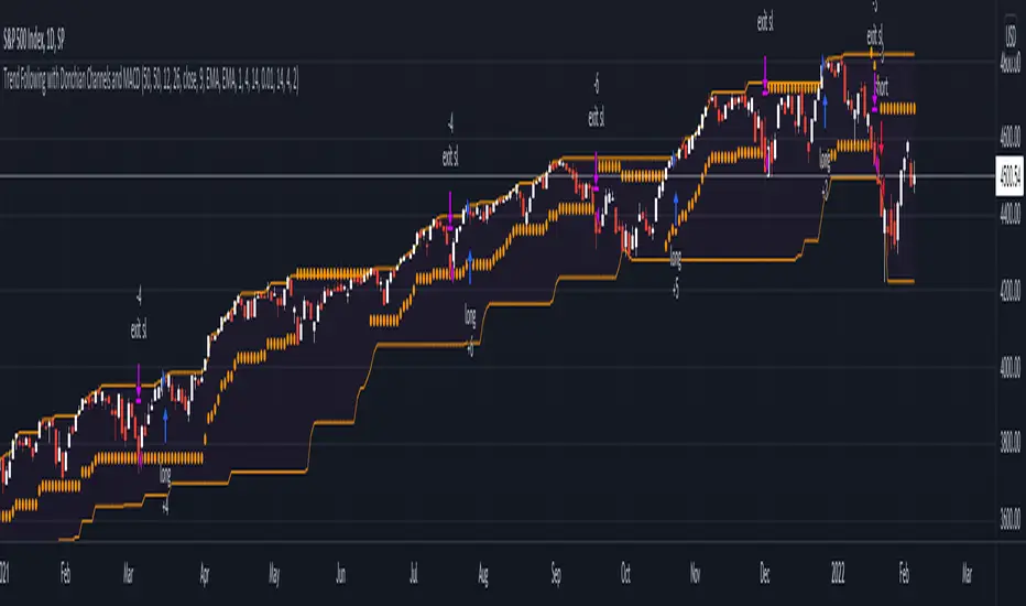
Trend Following with Donchian Channels and MACDThis is a trend following system based on the Donchian Channels. Instead of using a simple moving average crossover, this system uses the MACD as the trendfilter:
Long positions:
* Price makes a new 50 day high,
* The MACD-line crosses above or is above the Signal-line.
* Both the MACD and the Signal-lines are above the zero-line.
Short positions:
* Price makes a new 50 day low,
* The MACD-line crosses below or is below the Signal-line.
* Both the MACD and the Signal-lines are below the zero-line.
Stoploss:
The initial and the trailing stoploss are 4 ATRs away from the price.
"Trailing stop" için komut dosyalarını ara
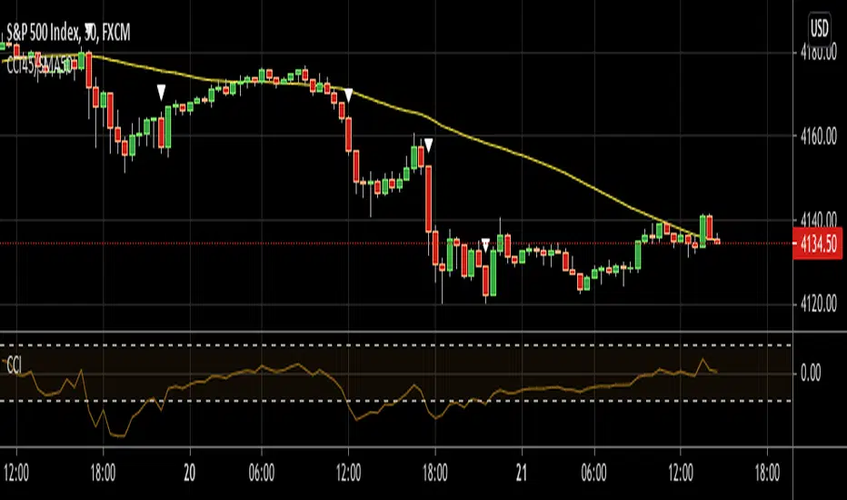
CCI45/SMA50 indy for 30 min SP500SPCFD:SPX
The script determines entry points using 45 period CCI and 50 period SMA.
Long condition: When CCI crosses up 150 treshold while price above 50 period SMA
Short condition: When CCI crosses down -150 treshold while price below 50 period SMA
Trades are executed above/below 1 point of high/low for long/short positions. Stops are just 1 point below/above of SMA. After 4 points of profit stops should be tightened. If you do not plan to hold the position for a long time, it can produce quick profit within 5-6 bars namely 2.5-3 hour. Otherwise you can manage the trade using SMA as trailing stop. This can be treated as a strategy of scalping which turns out a trend trading eventually if conditions good.
Have a nice trading
[fareid] Quick Backtest Framework█ OVERVIEW
This Framework allows Pine Coders to quickly code Study() based signal/strategy and validate its viability before proceed to code with more advance/complex customized rules for entry, exit, trailstop, risk management etc..
This is somewhat an upgraded version of my earlier personal template with different strategy used, cleaner code
and additional features.
█ USE CASES
- You have an idea for trade signal and need a quick way to verify its potential before writing lengthy/complicated code
- You found a study script for trading signal in public library and want to validate it profitability with minimum effort before including it in your trading playbook
█ FEATURES
- Alert: Ready to use alert function based on signals from your custom indicator.
- Visual Backtest: Auto-plot entry, stop-loss and take profit for simple strategy performance analysis
- Backtest Statistic: Provide basic key metrics based on backtest strategy
- BTE External Signal Protocol: Ready to use code that will supply required state to PineCoders Backtesting & Trading Engine if you wish to have more advance and sophisticated backtesting engine
Notes: All of the above features have On/Off toggle
█ Description & How To Use
This Framework consist of 5 Modules but you only need to edit the first 2 Modules:
Module1: Indicator
Module2: Framework Input Protocol
Module3: Alert
Module4: Backtest
Module5: Backtest & Trading Engine
Tips: The source-code includes collapsible block by module for easy navigating
Module1: Indicator:
-----------------------------------------------------------------------------------
Main Module. Place custom indicator input parameter/calculation/indicator plotting here
Sample Strategy: Double MACD Crossover
MACD Signal: 1st MACD Cross above signal line indicate Buy Signal
1st MACD Cross below signal line indicate Sell Signal
MACD Filter: 2nd MACD is above 0 line indicate Uptrend
2nd MACD is below 0 line indicate Downtrend
Module2: Framework Input Protocol:
-----------------------------------------------------------------------------------
Use this module to connect main indicator/signal calculated in Module1 to the rest of the framework's module
4 variables needed to be defined here:
1. Uptrend
2. Dntrend
3. BuySignal
4. SellSignal
i'm not sure how to place a code snippet here to show you example so in the source code i already put a comment in Module2 on which part u need to edit. I hope its pretty simple to use.
Module3: Alert Module Description:
-----------------------------------------------------------------------------------
As long as the variables in Module2 properly defined, the alert module is ready to use without any further modification.
Input:
Enable Alert --> Enable TV's alert and plot signal to chart
Alert Type --> Set to take Buy only, Sell only or Both alert
Module4: Backtest Module Description:
-----------------------------------------------------------------------------------
As long as the variables in Module2 properly defined, the backtest module is ready to use without any further modification.
Input:
Backtest Stat --> Enable Backtest Statistic Label
Backtest Visual --> Enable Backtest visual simulation
Backtest Type --> Set to take Buy only or Sell only or both
SL Type -->
ATR : Set SL in ATR times Multiplier below entry price
Fixed : Set SL in fixed point below entry point (in 'Dollar'). e.g. for Stocks -> 0.5 equals to 50cent while for EURUSD currency -> 0.005 equal to 50 pips
HiLo Bar: Set SL at highest/lowest wick of previous bar plus/minus Fixed point. e.g. EURUSD HiLo=3 and Fixed Point = 0.0005, buy trade will place SL 5 Pips below lowest of previous 3 bar
SL ATR Multi --> Set Lookback Period used for SL's ATR calculation
SL ATR Multi --> Set ATR Multiplier for SL
SL Fixed --> Set Fixed Level for SL
SL Bar --> Set Number of previous bar to check for SL placement
TP RR Ratio --> Set TP based on RR multiplier. e.g. 2 means TP level will be twice further from entry point compared to Entry-SL distance.
Notes: The point is for preliminary testing, so it only supports 1 trade at a time and no Trailing Stop
Module5: Backtest & Trading Engine Description:
-----------------------------------------------------------------------------------
As long as the variables in Module2 properly defined, the Pinecoders BTE module is ready to use without any further modification.
Input:
External Signal Protocol --> Set ESP State to send to "Backtesting & Trading Engine "
Signal With Filter --> Use this to send entry signal that already filtered by this study indicator (without stoploss level)
Signal Without Filter --> Use this to send raw entry signal that are NOT YET FILTERED by this study indicator (without stoploss level)
Signal and Stop With Filter --> Use this to send entry signal WITH StopLoss that already filtered by this study indicator (with stoploss level)
Signal and Stop Without Filter --> Use this to send raw entry signal WITH StopLoss that are NOT YET FILTERED by this study indicator (with stoploss level)
Notes: Backtesting & Trading Engine already have built-in Filter, Entries and Stop Level. e.g. Unselect all their filter state if only want to use custom filter and make sure send Signal with Filter (with or without SL level)
█ DISCLAIMER:
This framework main objective is to create my personal indicator template so that i just have to modify the indicator module for preliminary testing in future.
The sample strategy included are for educational purpose only. Use at your own risk
credit: LucF/PineCoders for a lot of his scripts that i use as a guide to complete this

Anti-Volume Stop LossFINALLY!
As everyone who tried to create, understand, or even find the Buff Pelz Dormeier Anti-volume stop-loss indicator knows that - it's not easy. Personally, I have partially, or perhaps completely figured out, the tips Buff had given in Investing with Volume Analysis book.
AVSL now is ready.
Please do some test and give me a feedback how it works in your trade strategy.
Anti-Volume stop loss - AVSL
from Investing with Volume Analysis book CHAPTER 20 • RISKY BUSINESS 253-256:
"It is important in any risk-management process to predetermine an objective decision point level (a stop loss) to exit, thereby protecting principal in case you are wrong. My objective sell point is determined by using a quantitative formula I refer to as Anti-Volume Stop Loss (AVSL). Having a quantitative, yet intelligent sell point eliminates the emotional struggles involved in deciding when to exit a position.
AVSL is a technical methodology that incorporates the concepts of support, volatility, and, most importantly, the inverse relationship between price and volume. The AVSL combines the concepts of the VPCI (Volume Price Confirmation Indicator) and John Bollinger’s Bollinger Bands to create a trailing stop loss.
AVSL = Lower Bollinger Band – (Price, Length, Standard Deviation)
Where:
Length = Round (3 + VPCI)
Price = Average (Lows × 1 / VPC × 1 / VPR, Length)
Standard Deviation = 2 × (VPCI × VM)
One of the most difficult decisions is determining what one’s maximum loss threshold should be. Some say 2 percent; others say 20 percent. I believe the more volatile a security, the looser the stop should be. A nonvolatile security, such as Coca-Cola, might move 7 percent a year, while a volatile security such as Google might move 7 percent in a day. If you use a 7 percent stop for Coca-Cola, it might take a year to be stopped out while the security underperforms.
However, if you use 7 percent for Google, you can be stopped out intraday, not allowing the investment an opportunity to develop. By using the lower Bollinger Band of the securities lows, the AVSL considers each individual security’s own volatility. Thus, a volatile security would be granted more room of the stocks low while a stable security would have a tighter leash (see Figure 20.7).
The next important step is employing the price-volume relationship into the calculation. Volume gauges the power behind price moves. In accounting for this, when a security is in an uptrend and has positive volume characteristics, it is given more room. However, if the security exhibits contracting volume characteristics, then the stop is tightened. In this way, if a negative news event affects an unhealthy security, the stop is tighter, thus preserving more of your profits.
However, if the negative news event affects a security whose price-volume relationship is healthy, the stop has been loosened, avoiding the temporary whipsaw of an otherwise strong position. In these ways, AVSL lets the market decide when to exit your position.
AVSL tailors each security for support, volatility, and the pricevolume relationship based on an investor’s time frame as calculated from the chart data. For example, my portfolio positions are continually re-evaluated with this AVSL methodology, which yields the possibility of raising the decision point threshold periodically based on the time frame of my investment objective. With my short-term Giddy-up portfolios, I use daily chart data and seek to raise my maximum loss stop on a daily basis.
My intermediate ETF and stock positions are calculated off of weekly data and then re-evaluated weekly. With my longer term stock portfolios, the decision point is calculated off data revised monthly. This analytical approach that uses measurable facts over emotion or gut instincts allows me to maintain my objectivity. Thus objectivity, not emotion, informs my investment decisions."
How look mine AVSL:
Price component = low × 1/VPC × 1/VPR : for VPC > 1 and VPC < -1 | low × 1 × 1/VPR : for 1 > VPC > 0 | low × -1 × 1/VPR : for 0 > VPC > -1
AVSL Price = sma((low × 1/VPC × 1/VPR) , length) / 100
length = round : for VPCI > 0 | round [ absolute ] : for VPCI < 0 | 3 : for VPCI=0
Standard Deviation = mult × VPCI × VM)
AVSL = sma(Actual low price - AWSL Price + Standard Deviation, 26)
It's hard to say is it the same as in Buff Pelz Dormeier book, but I encourage you to modify the script for better results.

Percent Drop from Highest HighBuy and hold investors may decide to use trailing stops to protect profits and capital from market crashes, especially during bull markets.
The purpose of this indicator is to hep investors to identify a location to place them. The indicator plots the highest high from 'x' bars ago. It then plots a trailing stop loss 'y' percent below that line.
The indicator enables its users to input different 'x' and 'y' values to observe what they think works best for them in different markets.
Users might choose to pair the indicator with trend confirming indicators, such as moving average cross overs, to determine that the market is trending and not ranging.
There is no magic in this indicator, only maths. Like every indicator, it has no ability to predict anything. Just because the market is doing one thing now, it might do something different later. The past does not equal the present nor the future. Make your own decisions and be responsible for them.
All the best to you and your family.

Breakout Trend Trading Strategy - V1Strategy in nutshell:
This strategy is made to be used in daily time-frames. Works better on trending instruments where volume is available. Hence, this is more suitable for trending shares rather than currencies, commodities and indexes where volume data is either not present or not reliable.
Breakout signifies the continuation of trend. Hence, trade in the direction of breakouts. Breakouts are calculated based on high volume and price movement in a day. This will be combined with few other conditions to generate buy and sell signals along with stop and compound targets. Supertrend is used for trend bias. Our buy and sell targets do not directly depend on the bias. But, entry criteria in opposite trend is made much difficult than that of trend direction. Further explanation of method and input parameters are explained below.
Backtesting parameters :
Capital and position sizing : Capital and position sizing parameters are set to test investing 2000 wholly on certain stock without compounding.
Initial Capital : 2000
Order Size : 100% of equity
Pyramiding : 1
ExitOnSignal : If unchecked exit is triggered solely on trailing stop
Trade Direction : Long, Short or All. Short condition is riskier than long conditions and often results in losses as per my observation. On most of the stocks trending up, strategy will not generate any short signals. This is achieved by comparing yearly high lows to previous two years to decide whether to allow short or long entries.
allowImmediateCompound : Applicable only if compounding/pyramiding is enabled in trade. If checked allows to place compounding orders immediately. If unchecked, it waits for stopline to cross order price before placing next compound.
Display Mode :
Targets : Whenever breakout happens, show marker for upTarget and downTarget
TargetChannel : Show up target and downtarget as a channel
Target With Stop : Along with targets, show also stop levels for breakouts
Up Channel : Channel created from UpTarget and respective stops
Down Channel : Channel created from DownTarget and respective stops
ShowTrailingStop : Shows trailing stop and compound lines when there is a trading position.
ShowTargetLevels : Shows Buy Sell target levels along with stop and compound lines. Trades are done as market orders. Hence, target levels are displayed after strategy makes the trade. Since only one order allowed per side without compounding, target, stop and compound levels are shown sometimes even without trade being made. These can be considered as entry levels if there is no existing position.
ShowPreviousLevels : Shows previous buy/sell target levels. When enabled, layout can look messy.
StopMultiplyer: To Set trailing stop loss.
BacktestYears: Number of years to include in backtest
So far my test cases are:
Positive : AAPL, AMZN, TSLA, RUN, VRT, ASX:APT
Negative Test Cases: WPL, WHC, NHC, WOW, COL, NAB (All ASX stocks)
Special test case: WDI
Negative test cases still show losses in backtesting. I have attempted including many conditions to eliminate or reduce the loss. But, further efforts has resulted in reduction in profits in positive cases as well. Still experimenting. Will update whenever I find improvements. Comments and suggestions welcome :)


Candle Type w/2Up + 2Dn v2.0This script builds on Candle Type w/2Up + 2Dn by incorporating signals for inside + up, outside + up, + rev strat set-ups. All of these can be turned off if they compete w/ other indicators or just clutter up the chart.
Briefly, the script works based on #thestrat developed by Rob Smith and the 1-2-3 bar script coded by @Crinklebine. Candle Type w/2Up + 2Dn is a "fork" of @Crinklebine's excellent indicator. I find the visualization of U-D-I-O (up/dn/inside/outside candles) easier to scan through 100's of charts than 1-2-3's. This is just personal preference, but they work based on the exact same principles. Performance is enhanced with a trend filter like @boardriderb's "TC" script or similar timeframe continuity filters based on the #thestrat developed by Rob Smith. I also prefer an ATR-based trailing stop; Rob recommends pSAR for trailing stops.
Together these indicators form a power system, but users are still responsible for their own trade management, entries & exits, risk profiles, stop loss, etc.

Volatility StopThis is a new version of the classic Volatility Stop originally published in 2014 by admin and written in Pine v1. While the code has evolved, its logic is identical. It is an ATR-based trend detector that can also be used as a stop. It belongs to the same family of indicators as:
• Charles Le Beau's Chandelier Exit ,
• Olivier Seban's Super Trend , and
• Sylvain Vervoort's Average True Range Trailing Stop .
Unlike the Chandelier Exit , Volatility Stop will not move against the trend.
This new version is written in Pine v4. The indicator can be used as a chart overlay, like the original. The calculations have been functionalized for easier reuse, so it is now easier to lift the logic out of the script and use it in others.
Features
• Choice of 2 color themes.
• Choice of display as a line, circles, diamonds or arrows. The line can be used with the other shapes. If no line is required, set its thickness to zero.
• Same default of length=20 and ATR factor=2 used in the original Volatility Stop.
• 3 alerts: on any trend change, or on changes into up or downtrends only. Alerts should be configured to trigger Once Per Bar Close .
Original version:
Look first. Then leap.

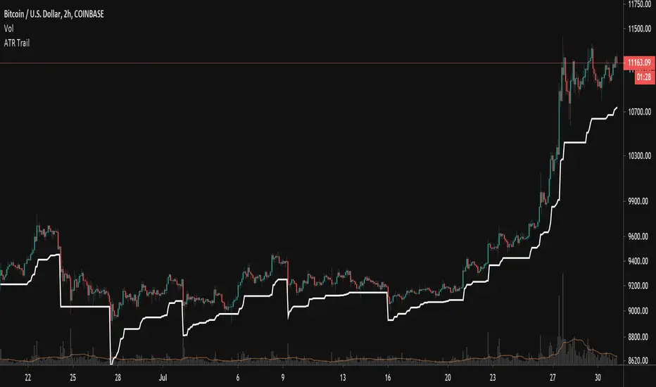
Trailing ATR StopsThis script plots a trailing stop of the ATR multiplied by a user-defined number. Since it is meant to be used as a trailing stop, the value doesn't fluctuate with the price as a normal ATR indicator does, but stays fixed unless price moves away from it. In that case it follows the price. If price crosses the stop level, it resets itself based on current price and starts trailing all over again.
User Settings:
Support - Use for a trailing stop while long
Resistance - Use for a trailing stop while short
Both - Acts like a channel and can spot periods of lower volatility
SAR Trend Trader w/ Alerts By: jhanson107This strategy utilizes Parabolic SAR (Stop and Reverse) along with EMA filtering to improve accuracy. Use the strategy to find optimal settings for the pair your are trading.
Long:
1. SAR below price action
2. Above slow EMA (Default 100 EMA)
3. Update trailing stop daily and exit trade once stopped out.
Short
1. SAR above price action
2. Below slow EMA (Default 100 EMA)
3. Update trailing stop daily and exit trade once stopped out.
White Bars = No trade zone which helps filter out bad trades compared to only using Parabolic SAR.

SAR Trend Trader Strategy By: jhanson107This strategy utilizes Parabolic SAR (Stop and Reverse) along with EMA filtering to improve accuracy. Use the strategy to find optimal settings for the pair your are trading.
Long:
1. SAR below price action
2. Above slow EMA (Default 100 EMA)
3. Update trailing stop daily and exit trade once stopped out.
Short
1. SAR above price action
2. Below slow EMA (Default 100 EMA)
3. Update trailing stop daily and exit trade once stopped out.
White Bars = No trade zone which helps filter out bad trades compared to only using Parabolic SAR.

Breakout Reversal Entry on WMA - NG1! Overnight ver 1This script is for learning purposes only
This strategy will plot arrows when price breaks so far above/below WMA. The strategy will enter when the price breaks away from WMA. All entries are reversals. Users can set WMA length and source; also the distance of the price away from WMA to enter. Adjustable bracket orders are placed for exit, with trailing stop or market stop choice. Last, users can set the time of day they want to enter a trade.
My Preference: I am testing this strategy on NG1! over night on 1 minute candle. with .003 on price drop/climb, I get entries almost every night. Also 10 tick stop and 5 tick profit seems backward to most, but with a high win/loss ratio, it performs quite well. Trailing stops generally help out as well.
INPUTS:
Length - The is the WMA length
Source - WMA source (High, Low, Open, Close...)
When Price Drops - This is the distance in ticks when the price drops away from WMA, an arrow is plotted, and reversal entry order is placed
When Price Climbs - Same as price drop, just in the opposite direction
Trailing Stop check box - Check if you want to place a trailing stop so many tick away from entry. Unchecked is Market (hard) stop so many ticks from entry.
Stop - Number of ticks away from entry a the stop or trailing stop is set (for NG 1 tick = $0.001)
Limit Out - Number of ticks away from entry a limit order is placed to take profits
Limit Time of day check box - check to use the time of day to limit what time of day order entry will occur.
Start/Stop Trades (Est Time) - First box is when the strategy will be allowed to start buying and stop is when the strategy will stop being allowed to buy. Sell orders continue until a stop or limit triggers an exit. These times are Eastern time zone
PROPERTIES:
Pyramiding - This feature will allow multiple entries to occur. If set to 1, the strategy should only trade 1 contract at a time. If set to 2, the strategy will enter a second order if entry requirements are met. This allows you to be holding 2 contracts. Basically on a good day, it will multiply your earnings, on a bad day, you'll just lose more. For testing, I keep this on 1.
TIPS:
- If you want to go long only, set "When Price Climbs" to an impossible number, like 10,000. It's not possible for NG to move $10 is a matter of minutes so it will not enter the market with a short order. Also keep in mind you can set different requirements for going long vs going short. If you think there is more pull on the market in a particular direction.

Trade Manager (Open Source Version)Hello my young padawans looking for the FORCE to get richer on your next trade
I got pinged at least three times today asking where the hell is the indicator of the day. You asked, I delivered :)
Here's your free open-source Trade Manager Version. My associates might kill me for sharing that one... anyway this is a real GIFT.
I won't share such quality indicators too often for FREE so hope you'll appreciate its value. It can really help with your day to day trading (on top of making your charts looking more awesome)
This is an even better version compared to my previous Trade Manager Trade-Manager . It's basically a standalone version, meaning you'll have to update with 2 lines your own indicator and follow my educational post from yesterday (pasted it below also) to learn how to do it
Please read this educational post I published for you before proceeding further : How-to-connect-your-indicator-with-the-Trade-Manager
From here you normally connected the data source of your own indicator to the Trade Manager. If not, here's a reminder of the article mentionned above
Step 1 - Update your indicator
For the screenshot you see above, I used this indicator : Two-MM-Cross-MACD/ . "But sir are you really advertising your other indicators here ??" ... hmmm.... YES but I gave them for free so ... stop complaining my friend :)
Somewhere in the code you'll have a LONG and a SHORT condition. If not, please go back to study trading for noobs (I'm kidding !!!)
So it should look to something similar
nUP = ma_crossover and macd_crossover
nDN = ma_crossunder and macd_crossunder
What you will need to add at the very end of your script is a Signal plot that will be captured by the Trade Manager. This will give us :
// Signal plot to be used as external
// if crossover, sends 1, otherwise sends -1
Signal = (nUP) ? 1 : (nDN) ? -1 : na
plot(Signal, title="Signal")
The Trade Manager engines expects to receive 1 for a bullishg signal and -1 for bearish .
Step 2 - Add the Trade Manager to your chart and select the right Data Source
I feel the questions coming so I prefer to anticipate :) When you add the Trade Manager to your chart, nothing will be displayed. THIS IS NORMAL because you'll have to select the Data Source to be "Signal"
Remember our Signal variable from the Two MM Cross from before, now we'll capture it and.....drumb rolll...... that's from that moment that your life became even more AWESOME
The Engine will capture the last signal from the MM cross or any indicator actually and will update the Stop Loss, Take Profit levels based on the parameters you set on the Trade Manager
It should work with any indicator as long as you're providing a plot Signal with values 1 and -1 . In any case, you can change the Trade Manager you'll find a better logic for your trading
Now let's cover the different parameters of the tool
It should be straightforward but better to explain everything here
+Label lines : if unchecked, no SL/TPs/... will be displayed
+Show Stop Loss Signal : Will display the stop loss label. You have the choice between three options :
By default, the Stop Loss is set to NONE. You'll have to select a different option to enable the Stop Loss for real
++Percentage : Will set the SL at a percent distance from the price
++Fixed : SL fixed at a static price
++Trailing % : Trailing stop loss based on percentage level
The following is a KEY feature and I got asked for it many times those past two days. I got annoyed of getting the same request so I just did it
++Trailing TP: Will move the Stop Loss if the take profit levels are hit
Example: if TP1 is hit, SL will be moved to breakeven. If TP2 is hit, SL will be moved from TP1 to TP2
+Take Profit 1,2,3 : Visually define the three Take Profit levels. Those are percentage levels .
Meaning if you set TP1 = 2, it will set the TP1 level 2% away from the entry signal
Please note that once a Take profit level is reached, it will magically disappear. This is to be expected
I'll share in the future a way more complete version with invalidation, stop loss/take profits based on indicator, take profit based on supports/resistances, ...
I believe is such a great tool because can be connected to any indicator. I confess that I tried it only with a few... if you find any that's not working with the Trade manager, please let me know and I'll have a look
PS
I want to give a HUUUUUUUGE shoutout to the PineCoders community who helped me finishing it
Wishing you all the best and a pleasant experience with my work
David

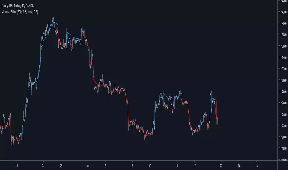
Modular Filter - Spot Trends And Smooth PriceIntroduction
This indicator can have a wide variety of usages, and since it is based on exponential averaging then the whole indicator can be made adaptive, thus ending up with a really promising tool. This indicator who can both smooth price and act as a trailing stop depending on user preferences, i tried to make it as reactive, stable and efficient as possible in order to both smooth and spot trends, lets view it more in depth.
The Indicator
line 8 and 9 create two bands, one upper and one lower, then based on certain conditions the indicator will only return a certain band or an average of both with different weights, this weight is controlled by the beta parameter, values of 1 will return a simple filter while values of 0 will return a classical trailing stop.
beta = 0
The indicator can use output values as input, thus using smoother values as input, in order to do so just check "Feedback", this help the overall output to be smoother as well as giving more long terms signals
The amount of feedback is controlled by the feedback weighting parameter, lower values will weight more the output values thus creating smoother results.
Feedback weighting of 0.2
Using beta = 0 thus having the indicator act as a trailing stop while having the feedback option activated return more long terms signals. Notes that the colors are based on the initial conditions of the indicator.
Conclusion
You can replace length and change alpha for any smoothing variable such as the efficiency ratio or anything with scale (1,0), same goes for beta and the feedback weighting parameter, this is why the indicator is "Modular" in addition of providing different usages. This indicator can look like cluster filters (smooth price monarch, forexguru) , filters with the ability to follow the price quite fine while being stables. I really hope you find an use to it.
Thanks for reading !
A.I.Driven TradersAI Model Trades for 20190612The entry and exit levels here are NOT derived from any specific indicator but are coming from our A.I. driven proprietary models.
This is an attempt at exploring the trading community here at TradingView and sharing our daily trading plans published at our site with the community here in the form a Pine Script - just starting and learning this platform. Please help point out any obvious errors or gotchas committed in the scripts. Thanks and have a great trading day!
**** The Trading Plan Published for today ****
>>>> Medium-Frequency Models: <<<<< For today, Wednesday 06/12, our medium-frequency models indicate using the 2895 as a pivot point - opening a long on a break above 2895, and opening a short on a break below 2895 (wait for a close on at least a five minute chart to determine the break), both sides with a 9-point trailing stop.
Note: For the trades to trigger, the breaks should occur during the regular session hours starting at 9:30am ET. By design, these models do NOT open any new positions after 3:45pm. Only one open position at any given time.
>>>>> Aggressive Intraday Models: <<<<< For today, Wednesday 06/12, our aggressive intraday models indicate going long on a break above 2892 or 2875 with an 6-point trailing stop, and going short on a break below 2887 or 2878 with an 8-point trailing stop.
Note: For the trades to trigger, the breaks should occur during regular session hours starting at 9:30am ET. Due to the intraday nature of these aggressive models, they indicate closing any open trades at 3:55pm and remaining flat into the session close. No opening of new positions after 3:45pm. Only one open position at any given time.

Flagging BandsIntroduction
A pun between the word flag and the adjective flagging (less dynamic) , this indicator have two bands who react faster when in contact to the price. Imagine you are under sheets, if you abruptly rise, the sheets will instantaneously go up, then if you abruptly get down, the sheets will fall slowly until being in contact with a surface, this is because of a type of friction called drag or air resistance , this force is described in fluid dynamics and i inspired myself from that for the creation of the indicator.
The indicator
The indicator is made of two bands, one upper band and one lower band, then a weighted average of each bands, this average is weighted depending on which band the price is closer. The length control the period of the indicator, in general higher lengths will create wider bands, you must consider that this parameter behave differently than other ones and may create slower results in comparison with other bands indicators while having the same length period.
The indicator can use a simple breakout methodology (see trailing stop part) but can sometime provide support and resistance points, in fact i believe that when the average variability/volatility of band A is higher than the average variability/volatility of band B and that the price cross band B then price will reverse its direction, this claim is not justified, research is needed.
Trailing Stop Mod
It is possible to make the indicator act as a trailing stop, in order to do so just tick the trailing stop mod box.
The average/bands will automatically disappear being replaced by the trailing stop.
Conclusion
I was just playing around when making the skeleton of the indicator, i hope the code is easy to understand, if you need some kind of explanation just pm me, i'm always open to help people/receive suggestions.
Best Regards

[Autoview][BackTest]Dual MA Ribbons R0.12 by JustUncleLThis is an implementation of a strategy based on two MA Ribbons, a Fast Ribbon and a Slow Ribbon. This strategy can be used on Normal candlestick charts or Renko charts (if you are familiar with them).
The strategy revolves around a pair of scripts: One to generate alerts signals for Autoview and one for Backtesting, to tune your settings.
The risk management options are performed within the script to set SL(StopLoss), TP(TargetProfit), TSL(Trailing Stop Loss) and TTP (Trailing Target Profit). The only requirement for Autoview is to Buy and Sell as directed by this script, no complicated syntax is required.
The Dual Ribbons are designed to capture the inferred behavior of traders and investors by using two groups of averages:
> Traders MA Ribbon: Lower MA and Upper MA (Aqua=Uptrend, Blue=downtrend, Gray=Neutral), with center line Avg MA (Orange dotted line).
> Investors MAs Ribbon: Lower MA and Upper MA (Green=Uptrend, Red=downtrend, Gray=Neutral), with center line Avg MA (Fuchsia dotted line).
> Anchor time frame (0=current). This is the time frame that the MAs are calculated for. This way 60m MA Ribbons can be viewed on a 15 min chart to establish tighter Stop Loss conditions.
Trade Management options:
Option to specify Backtest start and end time.
Trailing Stop, with Activate Level (as % of price) and Trailing Stop (as % of price)
Target Profit Level, (as % of price)
Stop Loss Level, (as % of price)
BUY green triangles and SELL dark red triangles
Trade Order closed colour coded Label:
>> Dark Red = Stop Loss Hit
>> Green = Target Profit Hit
>> Purple = Trailing Stop Hit
>> Orange = Opposite (Sell) Order Close
Trade Management Indication:
Trailing Stop Activate Price = Blue dotted line
Trailing Stop Price = Fuschia solid stepping line
Target Profit Price = Lime '+' line
Stop Loss Price = Red '+' line
Dealing With Renko Charts:
If you choose to use Renko charts, make sure you have enabled the "IS This a RENKO Chart" option, (I have not so far found a way to Detect the type of chart that is running).
If you want non-repainting Renko charts you MUST use TRADITIONAL Renko Bricks. This type of brick is fixed and will not change size.
Also use Renko bricks with WICKS DISABLED. Wicks are not part of Renko, the whole idea of using Renko bricks is not to see the wick noise.
Set you chart Time Frame to the lowest possible one that will build enough bricks to give a reasonable history, start at 1min TimeFrame. Renko bricks are not dependent on time, they represent a movement in price. But the chart candlestick data is used to create the bricks, so lower TF gives more accurate Brick creation.
You want to size your bricks to 2/1000 of the pair price, so for ETHBTC the price is say 0.0805 then your Renko Brick size should be about 2*0.0805/1000 = 0.0002 (round up).
You may find there is some slippage in value, but this can be accounted for in the Backtest by setting your commission a bit higher, for Binance for example I use 0.2%
Special thanks goes to @CryptoRox for providing the initial Risk management Framework in his "How to automate this strategy for free using a chrome extension" example.

EMA StrategyThis strategy is in testing and development.
**USE AT YOUR OWN RISK. **
This defaults to a 13/48 EMA using the closing price. When the fast EMA crosses above the slow it triggers a buy. When it crosses below the slow EMA it triggers a sell and potentially a short, but that is not implemented. Stops, trailing stops, and pyramiding to be added. The purpose of this strategy is to signal recommended entry and exit point and back test whether the strategy works. It is not intended to be an automated buy/sell script.
* stop loss added. Not yet configurable from the settings panel. Defaults to 8% from the entry price.
TODO:
Add the ability to configure the stop-loss level in the settings panel
Add trailing stop functionality
Add profit taking, likely configurable sell targets (2:1 risk to reward gain for example)
Add another signal or two to help improve odds of making a winning trade.

VWAP Long Entry PROVWAP Long Entry PRO - Instruction Manual
Overview
VWAP Long Entry PRO is a Pine Script v6 indicator designed for day traders following Andrew Aziz's VWAP trading methodology from "How to Day Trade for a Living." The indicator identifies high-probability long entry opportunities when stocks bounce off VWAP with proper trend, volume, and timing confirmation.
What This Indicator Does
The indicator monitors multiple conditions simultaneously and alerts you only when ALL criteria are met for a valid VWAP long entry:
1. ✅ Price is near VWAP (within customizable proximity)
2. ✅ Price crosses above VWAP (bullish candle confirmation)
3. ✅ Uptrend confirmed (EMA 20 > EMA 50)
4. ✅ Volume spike present (volume > 1.5x average)
5. ✅ Within optimal trading hours (default: first 2 hours after market open)
Visual Elements on the Chart
1. VWAP Line (Yellow)
* Shows the Volume Weighted Average Price for the current session
* Acts as dynamic support/resistance
2. EMA Lines
* Blue Line: 20-period Exponential Moving Average
* Red Line: 50-period Exponential Moving Average
* Trend is bullish when blue is above red
3. Green Triangle Markers
* Appear below candles when ALL entry conditions are met
* These are your entry signals
4. Background Colors
* Light Yellow Background: Price is within proximity zone of VWAP
* Light Red Background: Price crossed VWAP but filters failed (helps identify missed opportunities)
5. Filter Status Table (Top Right)
Real-time dashboard showing current status of all filters:
Filter Status
Trend ✓ (green) or ✗ (red)
Volume ✓ (green) or ✗ (red)
Time ✓ (green) or ✗ (red)
Near VWAP ✓ (green) or ✗ (red)
Entry OK ✓ GO (lime) or ✗ (orange)
How to Use the Indicator
Step 1: Apply to Your Watchlist
1. Add VWAP Long Entry PRO to charts of stocks on your morning gappers watchlist
2. Use 1-minute, 2-minute, or 5-minute timeframes
3. Monitor multiple stocks simultaneously
Step 2: Wait for Setup
Watch the Filter Status Table in the top right corner. A valid entry requires:
* All filters showing green ✓
* "Entry OK" showing ✓ GO in lime/green
Step 3: Execute the Trade
When a green triangle appears below a candle:
* Entry: Enter long at or near the close of that candle
* Stop Loss: Place stop just below VWAP (typically 2-5 cents below)
* Profit Target: Use resistance levels, previous highs, or VWAP + ATR
Step 4: Manage the Trade
* Hold as long as price stays above VWAP
* Exit if price closes back below VWAP
* Scale out at resistance levels
Customizable Settings
Access settings by clicking the gear icon next to the indicator name.
VWAP Proximity
* Default: 0.002 (0.2%)
* Purpose: Defines how close price must be to VWAP
* Adjust If:
* Too many signals → increase (e.g., 0.001 = 0.1%)
* Too few signals → decrease (e.g., 0.003 = 0.3%)
Filters Group
Trend Filter
* Use Trend Filter: Toggle on/off
* EMA 20 Length: Default 20
* EMA 50 Length: Default 50
* Purpose: Ensures you're trading with the trend
* Disable If: Trading reversals or range-bound stocks
Volume Filter
* Use Volume Filter: Toggle on/off
* Volume Multiplier: Default 1.5 (volume must be 1.5x average)
* Volume Average Period: Default 20 bars
* Purpose: Confirms institutional participation
* Adjust If:
* Too restrictive → lower to 1.2x
* Need stronger confirmation → increase to 2.0x
Time Filter
* Use Time Filter: Toggle on/off
* Start Hour (EST): Default 9
* Start Minute: Default 30
* Hours to Trade: Default 2
* Purpose: Focus on highest probability time window (9:30-11:30 AM EST)
* Adjust If:
* Trading afternoon momentum → extend hours to 4-6
* Power hour trading → change start to 15:00, 1 hour
Alert Setup
Creating an Alert
1. Click the Alert Icon (clock) in top toolbar
2. Condition: Select "VWAP Long Entry PRO"
3. Alert Trigger: Choose "VWAP Long Entry PRO"
4. Options: Select "Once Per Bar Close"
5. Expiration: Set to desired timeframe (default: 60 days)
6. Alert Actions: Enable:
* ✓ Notify on App
* ✓ Show Popup
* ✓ Send Email (optional)
* ✓ Play Sound
7. Message: The default message includes:
* Ticker symbol
* Close price
* VWAP value
* Confirmation that all filters passed
Multi-Symbol Alert
To monitor multiple stocks with one alert:
1. In the alert creation dialog, use the Symbol dropdown
2. Select multiple tickers from your watchlist
3. The alert will fire when ANY of those stocks meet the criteria
Trading Strategy
Based on Andrew Aziz's VWAP Methodology
Setup Requirements:
* Stock must be "in play" (gap, news, high relative volume from morning scanner)
* Price pulls back to VWAP during the trading day
* VWAP acts as support for longs (or resistance for shorts)
Entry Rules:
1. Wait for price to approach VWAP
2. Confirm VWAP as support with a bullish candle closing above it
3. Enter long on confirmation candle close or next candle open
4. All filters (trend, volume, time) must be green
Stop Loss:
* Place stop 2-5 cents below VWAP
* Adjust based on stock volatility and your risk tolerance
Profit Targets:
* First target: Previous resistance or swing high
* Second target: Daily pivot or Fibonacci extension
* Trailing stop: Move stop to breakeven once up 1:1 risk/reward
Risk Management:
* Risk 1-2% of account per trade
* Position size based on distance from stop loss
* Aim for 2:1 or 3:1 reward-to-risk ratio
Common Scenarios
Scenario 1: Clean VWAP Bounce
* All filters green ✓
* Price pulls back to VWAP
* Green triangle appears
* Action: Enter long immediately
Scenario 2: Failed Volume
* Trend ✓, Time ✓, Near VWAP ✓
* Volume ✗ (red X)
* Action: Wait for volume increase or skip trade
Scenario 3: Wrong Time Window
* All filters green except Time ✗
* Action: If you trade mid-day, consider extending time window in settings
Scenario 4: Downtrend
* Trend ✗ (EMA 20 < EMA 50)
* Action: Skip long entry; consider short setup instead
Scenario 5: False Breakout
* Light red background appears (filters failed)
* Price crossed VWAP but no confirmation
* Action: No entry; indicator correctly filtered out weak signal
Best Practices
1. Pre-Market Preparation
* Run your gappers scanner at 9:00 AM EST
* Identify 3-5 stocks "in play"
* Add VWAP Long Entry PRO to each chart
* Set up alerts for your watchlist
2. Chart Timeframe Selection
* 1-minute: Scalping, high-frequency entries (more signals, more noise)
* 2-minute: Balanced (recommended for beginners)
* 5-minute: Swing entries, fewer but higher-quality signals
3. Combine with Price Action
The indicator is a filter and alert system, not a complete strategy. Also consider:
* Support/resistance levels
* Candlestick patterns (hammer, engulfing)
* Overall market trend (SPY, QQQ)
* Stock-specific news and catalysts
4. Backtesting
* Use TradingView's Bar Replay feature
* Review past signals on your favorite stocks
* Adjust filter settings based on your results
* Document win rate and average R:R
5. Paper Trading First
* Test the indicator with paper trading for 1-2 weeks
* Track all signals and outcomes
* Refine settings before risking real capital
Troubleshooting
Problem: No Signals Appearing
Solutions:
* Check if all filters are enabled (they may be too restrictive)
* Verify stock has sufficient volume and volatility
* Try increasing VWAP proximity from 0.2% to 0.3%
* Disable time filter if trading mid-day
* Check if stock is actually near VWAP on chart
Problem: Too Many Signals
Solutions:
* Decrease VWAP proximity from 0.2% to 0.1%
* Increase volume multiplier from 1.5x to 2.0x
* Enable all filters (trend, volume, time)
* Use 5-minute chart instead of 1-minute
Problem: Filter Status Table Not Visible
Solutions:
* Scroll chart to right (table is in top right corner)
* Check if indicator is loaded (should appear in indicator list on left)
* Refresh chart and re-add indicator
* Close other overlapping indicators
Problem: Alert Not Firing
Solutions:
* Verify alert is set to "Once Per Bar Close" (not "Only Once")
* Check alert hasn't expired
* Ensure correct symbols are selected in alert
* Confirm indicator is applied to chart with alert
Limitations
What This Indicator Does NOT Do:
* ❌ Automatically enter/exit trades
* ❌ Calculate position size
* ❌ Account for fundamental news or earnings
* ❌ Work on stocks without sufficient liquidity
* ❌ Guarantee profitable trades
When NOT to Use:
* Pre-market or after-hours (VWAP resets at market open)
* Low-volume penny stocks (< 100K daily volume)
* Stocks without clear trend or catalyst
* During major news events or FOMC meetings
* First 5 minutes after market open (price discovery phase)
Example Trade Walkthrough
Stock: XYZ (from morning gappers, +5% gap on earnings)
Time: 10:15 AM EST
Timeframe: 2-minute chart
Filter Status Table Shows:
* Trend: ✓ (EMA 20 > EMA 50)
* Volume: ✓ (2.3x average)
* Time: ✓ (within 9:30-11:30 window)
* Near VWAP: ✓ (price at $50.05, VWAP at $50.00)
* Entry OK: ✗ (waiting for bullish close)
Next Candle:
* Opens at $50.02
* Drops to $49.98 (testing VWAP)
* Closes at $50.08 (bullish candle, above VWAP)
* Green triangle appears!
* Entry OK: ✓ GO
Trade Execution:
* Entry: $50.10 (next candle open)
* Stop Loss: $49.95 (5 cents below VWAP)
* Risk: $0.15 per share
* Target 1: $50.40 (previous resistance) = 2:1 R:R
* Target 2: $50.70 (daily high) = 4:1 R:R
Outcome:
* Price rallies to $50.45
* Scale out 50% at Target 1
* Move stop to breakeven ($50.10)
* Exit remaining 50% at $50.65
* Result: Profitable trade with 3:1 average R:R
Frequently Asked Questions
Q: Can I use this for short entries?
A: The current version is for long entries only. For shorts, you'd need to reverse the logic (price rejecting VWAP as resistance, downtrend, etc.).
Q: What stocks work best with this indicator?
A: Mid-cap momentum stocks ($1B-$10B market cap), price $10-$100, daily volume > 1M, with a clear catalyst (earnings, news, sector move).
Q: Can I trade this on daily or weekly charts?
A: No. VWAP is an intraday indicator that resets each trading day. Use only on intraday timeframes (1m, 2m, 5m, 15m, 30m).
Q: Should I take every signal?
A: No. Use the indicator as a filter, not a mechanical system. Consider overall market conditions, stock-specific catalysts, and your own price action analysis.
Q: How accurate is this indicator?
A: Accuracy depends on market conditions, stock selection, and your execution. Expect 50-65% win rate with proper 2:1+ risk/reward, similar to Aziz's methodology.
Resources
* Book: "How to Day Trade for a Living" by Andrew Aziz
* VWAP Strategy: Focus on Chapters 7.6 (VWAP Strategy) and supporting examples
* Community: Bear Bull Traders (www.bearbulltraders.com)
* Practice: Use TradingView's Bar Replay and Paper Trading features
Support & Updates
For questions, issues, or feature requests, refer to the TradingView script comments or the Bear Bull Traders community.
Version: 1.0
Pine Script Version: v6
Last Updated: December 30, 2025
Disclaimer: This indicator is for educational purposes only. Trading involves substantial risk. Past performance does not guarantee future results. Always practice proper risk management and never risk more than you can afford to lose.
1. www.tradingview.com

PA SystemPA System
短简介 Short Description(放在最上面)
中文:
PA System 是一套以 AL Brooks 价格行为为核心的策略(Strategy),将 结构(HH/HL/LH/LL)→ 回调(H1/L1)→ 二次入场(H2/L2 微平台突破) 串成完整可回测流程,并可选叠加 BoS/CHoCH 结构突破过滤 与 Liquidity Sweep(扫流动性)确认。内置风险管理:定风险仓位、部分止盈、保本、移动止损、时间止损、冷却期。
English:
PA System is an AL Brooks–inspired Price Action strategy that chains Market Structure (HH/HL/LH/LL) → Pullback (H1/L1) → Second Entry (H2/L2 via Micro Range Breakout) into a complete backtestable workflow, with optional BoS/CHoCH structure-break filtering and Liquidity Sweep confirmation. Built-in risk management includes risk-based sizing, partial exits, breakeven, trailing stops, time stop, and cooldown.
⸻
1) 核心理念 Core Idea
中文:
这不是“指标堆叠”,而是一条清晰的价格行为决策链:
结构确认 → 回调出现 → 小平台突破(二次入场)→ 风控出场。
策略把 Brooks 常见的“二次入场”思路程序化,同时用可选的结构突破与扫流动性模块提升信号质量、减少震荡误入。
English:
This is not an “indicator soup.” It’s a clear price-action decision chain:
Confirmed structure → Pullback → Micro-range breakout (second entry) → Risk-managed exits.
The system programmatically implements the Brooks-style “second entry” concept, and optionally adds structure-break and liquidity-sweep context to reduce chop and improve trade quality.
⸻
2) 主要模块 Main Modules
A. 结构识别 Market Structure (HH/HL/LH/LL)
中文:
使用 pivot 摆动点确认结构,标记 HH/HL/LH/LL,并可显示最近一组摆动水平线,方便对照结构位置。
English:
Uses confirmed pivot swings to label HH/HL/LH/LL and optionally plots the most recent swing levels for clean structure context.
B. 状态机 Market Regime (State Machine + “Always In”)
中文:
基于趋势K强度、EMA关系与波动范围,识别市场环境(Breakout/Channel/Range)以及 Always-In 方向,用于过滤不合适的交易环境。
English:
A lightweight regime engine detects Breakout/Channel/Range and an “Always In” directional bias using momentum and EMA/range context to avoid low-quality conditions.
C. 二次入场 Second Entry Engine (H1→H2 / L1→L2)
中文:
• H1/L1:回调到结构附近并出现反转迹象
• H2/L2:在 H1/L1 后等待最小 bars,然后触发 Micro Range Breakout(小平台突破)并要求信号K收盘强度达标
这一段是策略的“主发动机”。
English:
• H1/L1: Pullback into structure with reversal intent
• H2/L2: After a minimum wait, triggers on Micro Range Breakout plus a configurable close-strength filter
This is the main “entry engine.”
D. 可选过滤器 Optional Filters (Quality Boost)
BoS/CHoCH(结构突破过滤)
中文: 可识别 BoS / CHoCH,并可要求“入场前最近 N bars 必须有同向 break”。
English: Detects BoS/CHoCH and can require a recent same-direction break within N bars.
Liquidity Sweeps(扫流动性确认)
中文: 画出 pivot 高/低的流动性水平线,检测“刺破后收回”的 sweep,并可要求入场前出现同向 sweep。
English: Tracks pivot-based liquidity levels, confirms sweeps (pierce-and-reclaim), and can require a recent sweep before entry.
E. FVG 可视化 FVG Visualization
中文: 提供 FVG 区域盒子与管理模式(仅保留未回补 / 仅保留最近N),主要用于区域理解与复盘,不作为强制入场条件(可自行扩展)。
English: Displays FVG boxes with retention modes (unfilled-only or last-N). Primarily for context/analysis; not required for entries (you can extend it as a filter/target).
⸻
3) 风险管理 Risk Management (Built-In)
中文:
• 定风险仓位:按账户权益百分比计算仓位
• SL/TP:基于结构 + ATR 缓冲,且限制最大止损 ATR 倍
• 部分止盈:到达指定 R 后减仓
• 保本:到达指定 R 后推到 BE
• 移动止损:到达指定 R 后开始跟随
• 时间止损:持仓太久不动则退出
• 冷却期:出场后等待 N bars 再允许新单
English:
• Risk-based sizing: position size from equity risk %
• SL/TP: structure + ATR buffer with max ATR risk cap
• Partial exits at an R threshold
• Breakeven at an R threshold
• Trailing stop activation at an R threshold
• Time stop to reduce chop damage
• Cooldown after exit to avoid rapid re-entries
⸻
4) 推荐使用方式 Recommended Usage
中文:
• 推荐从 5m / 15m / 1H 开始测试
• 想更稳:开启 EMA Filter + Break Filter + Sweep Filter,并提高 Close Strength
• 想更多信号:关闭 Break/Sweep 过滤或降低 Swing Length / Close Strength
• 回测时务必设置合理的手续费与滑点,尤其是期货/指数
English:
• Start testing on 5m / 15m / 1H
• For higher quality: enable EMA Filter + Break Filter + Sweep Filter and increase Close Strength
• For more signals: disable Break/Sweep filters or reduce Swing Length / Close Strength
• Use realistic commissions/slippage in backtests (especially for futures/indices)
⸻
5) 重要说明 Notes
中文:
结构 pivot 需要右侧确认 bars,因此结构点存在天然滞后(确认后不会再变)。策略逻辑尽量避免不必要的对象堆叠,并对数组/对象做了稳定管理,适合长期运行与复盘。
English:
Pivot-based structure requires right-side confirmation (inherent lag; once confirmed it won’t change). The script is designed for stability and resource-safe object management, suitable for long sessions and review.
⸻
免责声明 Disclaimer(建议原样保留)
中文:
本脚本仅用于教育与研究目的,不构成任何投资建议。策略回测结果受市场条件、手续费、滑点、交易时段、数据质量等影响显著。使用者需自行验证并承担全部风险。过往表现不代表未来结果。
English:
This script is for educational and research purposes only and does not constitute financial advice. Backtest results are highly sensitive to market conditions, fees, slippage, session settings, and data quality. Use at your own risk. Past performance is not indicative of future results.

Rate Trail IndicatorRate Trail Indicator Precision Trailing Stop & Multi-Timeframe Highs
Description The Rate Trail Indicator V2 is a professional-grade risk management tool designed to declutter your charts while providing precise, dynamic stop-loss levels. Unlike traditional indicators that paint a continuous "trail" or history across the chart, this script utilizes a Single Line visual approach. It draws only the currently active stop-loss level as a distinct horizontal line, keeping your workspace clean and focused on current price action.
This updated version now includes extensive Multi-Timeframe (MTF) Support, allowing you to overlay key Intraday and Higher Timeframe (HTF) highs directly on your chart.
Key Features Clean "Single Line" Visuals: Removes historical noise by plotting only the active stop-loss level and a dedicated price label. Dual Logic Modes: Percentage Mode: Classic trailing stop based on a percentage drop from the high. Renko Mode: Volatility-based stop that counts exact "Bricks" (supports decimals like 1.5 bricks). Dynamic Reset: The stop trails the "Lifetime High" of the current trend. If the stop is breached, it automatically resets to the current price to begin a new trail immediately. MTF High Breakout Levels: Optional toggles to display previous Intraday Highs (2H, 4H, 6H, 12H) and Historical Highs (1W, 2W, 1M, 3M). Rolling 3-Month Logic: The 3M level now uses a "Rolling" lookback (Highest of the last 3 monthly candles) rather than a fixed calendar quarter, ensuring the data is always recent and relevant. Full Customization: Control line styles (Solid, Dashed, Dotted), colors, and widths for every level independently via the inputs.
How to Use & Settings
1. Main Trailing Stop Setup Configure your primary risk line (Red Line) in the "Main Trailing Stop" group. Stop-Loss Mode: Select Percentage for standard equity/crypto trading (e.g., 2% trail) or Renko Boxes for Renko charts. Renko Boxes Down: Enter the number of bricks to trail. You can use decimals (e.g., 1.5) for fine-tuning. Use Fixed Lookback?: Unchecked (Default): The script tracks the "Infinite High" since the last reset. This is ideal for catching long trends. Checked: The script only looks at the highest price of the last X bars. This creates a more "rolling" stop-loss.
2. Intraday & Historical Highs (Resistance/Breakout) Enable up to eight additional lines to see where the price peaked on other timeframes. These act as strong breakout or resistance levels. Intraday Highs: Show the high of the previous 2H, 4H, 6H, or 12H session. 1W / 1M Highs: The highest price of the previous Week or Month. 2W High: The highest price of the last 2 Weeks . 3M High (Updated): The highest price of the last 3 Months (Rolling). This updates monthly, ensuring you aren't looking at data that is 6 months old.
3. Alerts You can set specific alerts to automate your trading or get notified instantly. Main Stop Breached: Fires when price closes below your trailing stop line. MTF High Cross: Fires when price crosses under any of the enabled Intraday or HTF High levels (2H, 4H, 1W, 3M, etc.).

A-Share Broad-Based ETF Dual-Core Timing System1. Strategy Overview
The "A-Share Broad-Based ETF Dual-Core Timing System" is a quantitative trading strategy tailored for the Chinese A-share market (specifically for broad-based ETFs like CSI 300, CSI 500, STAR 50). Recognizing the market's characteristic of "short bulls, long bears, and sharp bottoms," this strategy employs a "Left-Side Latency + Right-Side Full Position" dual-core driver. It aims to safely bottom-fish during the late stages of a bear market and maximize profits during the main ascending waves of a bull market.
2. Core Logic
A. Left-Side Latency (Rebound/Bottom Fishing)
Capital Allocation: Defaults to 50% position.
Philosophy: "Buy when others fear." Seeks opportunities in extreme panic or momentum divergence.
Entry Signals (Triggered by any of the following):
Extreme Panic: RSI Oversold (<30) + Price below Bollinger Lower Band + Bullish Candle Close (Avoid catching falling knives).
Oversold Bias: Price deviates more than 15% from the 60-day MA (Life Line), betting on mean reversion.
MACD Bullish Divergence: Price makes a new low while MACD histogram does not, accompanied by strengthening momentum.
B. Right-Side Full Position (Trend Following)
Capital Allocation: Aggressively scales up to Full Position (~99%) upon signal trigger.
Philosophy: "Follow the trend." Strike heavily once the trend is confirmed.
Entry Signals (All must be met):
Upward Trend: MACD Golden Cross + Price above 20-day MA.
Breakout Confirmation: CCI indicator breaks above 100, confirming a main ascending wave.
Volume Support: Volume MACD Golden Cross, ensuring price increase is backed by volume.
C. Smart Risk Control
Bear Market Exhaustion Exit: In a bearish trend (MA20 < MA60), the strategy does not "hold and hope." It immediately liquidates left-side positions upon signs of rebound exhaustion (breaking below MA20, touching MA60 resistance, or RSI failure).
ATR Trailing Stop: Uses Average True Range (ATR) to calculate a dynamic stop-profit line that rises with the price to lock in profits.
Hard Stop Loss: Forces a stop-loss if the left-side bottom fishing fails and losses exceed a set ATR multiple, preventing deep drawdowns.
3. Recommendations
Target Assets: High liquidity broad-based ETFs such as CSI 300 ETF (510300), CSI 500 ETF (510500), ChiNext ETF (159915), STAR 50 ETF (588000).
Timeframe: Daily Chart.
