ULTIMATE ICHIMOKU TRADING SUITEThis is an update of "Uncle Mo's Ultimate Ichimoku V1"
Main features:
2 x Ichimoku Cloud
5 x EMA
2 x MA
1 x HullMA
Williams Fractal
Bollinger Bands - ***NEW***
ATR - ***NEW***
PSAR - ***NEW***
Candlestick Patterns - ***NEW***
Price Action Bars- ***NEW***
List of credits:
@br0qn for the Ichimoku
@RicardoSantos for the Bill Williams Fractal
@EmilianoMesa for the EMAs/MAs
@mohamed982 for the HullMA
@ymaheshreddy4u for the Bollinger Bands
@ChrisMoody for the Price Action Bars and PSAR
@HPotter for the ATR
@repo32 for the Candlestick Patterns
The script is open source and free to use. Feel free to change it around to suit your needs.
***If you copy & paste code from other traders to make your own script, please do remember to give them credit for their amazing work.***
Happy trading!
"N+credit最新动态" için komut dosyalarını ara

Small Business Economic Conditions - Statistical Analysis ModelThe Small Business Economic Conditions Statistical Analysis Model (SBO-SAM) represents an econometric approach to measuring and analyzing the economic health of small business enterprises through multi-dimensional factor analysis and statistical methodologies. This indicator synthesizes eight fundamental economic components into a composite index that provides real-time assessment of small business operating conditions with statistical rigor. The model employs Z-score standardization, variance-weighted aggregation, higher-order moment analysis, and regime-switching detection to deliver comprehensive insights into small business economic conditions with statistical confidence intervals and multi-language accessibility.
1. Introduction and Theoretical Foundation
The development of quantitative models for assessing small business economic conditions has gained significant importance in contemporary financial analysis, particularly given the critical role small enterprises play in economic development and employment generation. Small businesses, typically defined as enterprises with fewer than 500 employees according to the U.S. Small Business Administration, constitute approximately 99.9% of all businesses in the United States and employ nearly half of the private workforce (U.S. Small Business Administration, 2024).
The theoretical framework underlying the SBO-SAM model draws extensively from established academic research in small business economics and quantitative finance. The foundational understanding of key drivers affecting small business performance builds upon the seminal work of Dunkelberg and Wade (2023) in their analysis of small business economic trends through the National Federation of Independent Business (NFIB) Small Business Economic Trends survey. Their research established the critical importance of optimism, hiring plans, capital expenditure intentions, and credit availability as primary determinants of small business performance.
The model incorporates insights from Federal Reserve Board research, particularly the Senior Loan Officer Opinion Survey (Federal Reserve Board, 2024), which demonstrates the critical importance of credit market conditions in small business operations. This research consistently shows that small businesses face disproportionate challenges during periods of credit tightening, as they typically lack access to capital markets and rely heavily on bank financing.
The statistical methodology employed in this model follows the econometric principles established by Hamilton (1989) in his work on regime-switching models and time series analysis. Hamilton's framework provides the theoretical foundation for identifying different economic regimes and understanding how economic relationships may vary across different market conditions. The variance-weighted aggregation technique draws from modern portfolio theory as developed by Markowitz (1952) and later refined by Sharpe (1964), applying these concepts to economic indicator construction rather than traditional asset allocation.
Additional theoretical support comes from the work of Engle and Granger (1987) on cointegration analysis, which provides the statistical framework for combining multiple time series while maintaining long-term equilibrium relationships. The model also incorporates insights from behavioral economics research by Kahneman and Tversky (1979) on prospect theory, recognizing that small business decision-making may exhibit systematic biases that affect economic outcomes.
2. Model Architecture and Component Structure
The SBO-SAM model employs eight orthogonalized economic factors that collectively capture the multifaceted nature of small business operating conditions. Each component is normalized using Z-score standardization with a rolling 252-day window, representing approximately one business year of trading data. This approach ensures statistical consistency across different market regimes and economic cycles, following the methodology established by Tsay (2010) in his treatment of financial time series analysis.
2.1 Small Cap Relative Performance Component
The first component measures the performance of the Russell 2000 index relative to the S&P 500, capturing the market-based assessment of small business equity valuations. This component reflects investor sentiment toward smaller enterprises and provides a forward-looking perspective on small business prospects. The theoretical justification for this component stems from the efficient market hypothesis as formulated by Fama (1970), which suggests that stock prices incorporate all available information about future prospects.
The calculation employs a 20-day rate of change with exponential smoothing to reduce noise while preserving signal integrity. The mathematical formulation is:
Small_Cap_Performance = (Russell_2000_t / S&P_500_t) / (Russell_2000_{t-20} / S&P_500_{t-20}) - 1
This relative performance measure eliminates market-wide effects and isolates the specific performance differential between small and large capitalization stocks, providing a pure measure of small business market sentiment.
2.2 Credit Market Conditions Component
Credit Market Conditions constitute the second component, incorporating commercial lending volumes and credit spread dynamics. This factor recognizes that small businesses are particularly sensitive to credit availability and borrowing costs, as established in numerous Federal Reserve studies (Bernanke and Gertler, 1995). Small businesses typically face higher borrowing costs and more stringent lending standards compared to larger enterprises, making credit conditions a critical determinant of their operating environment.
The model calculates credit spreads using high-yield bond ETFs relative to Treasury securities, providing a market-based measure of credit risk premiums that directly affect small business borrowing costs. The component also incorporates commercial and industrial loan growth data from the Federal Reserve's H.8 statistical release, which provides direct evidence of lending activity to businesses.
The mathematical specification combines these elements as:
Credit_Conditions = α₁ × (HYG_t / TLT_t) + α₂ × C&I_Loan_Growth_t
where HYG represents high-yield corporate bond ETF prices, TLT represents long-term Treasury ETF prices, and C&I_Loan_Growth represents the rate of change in commercial and industrial loans outstanding.
2.3 Labor Market Dynamics Component
The Labor Market Dynamics component captures employment cost pressures and labor availability metrics through the relationship between job openings and unemployment claims. This factor acknowledges that labor market tightness significantly impacts small business operations, as these enterprises typically have less flexibility in wage negotiations and face greater challenges in attracting and retaining talent during periods of low unemployment.
The theoretical foundation for this component draws from search and matching theory as developed by Mortensen and Pissarides (1994), which explains how labor market frictions affect employment dynamics. Small businesses often face higher search costs and longer hiring processes, making them particularly sensitive to labor market conditions.
The component is calculated as:
Labor_Tightness = Job_Openings_t / (Unemployment_Claims_t × 52)
This ratio provides a measure of labor market tightness, with higher values indicating greater difficulty in finding workers and potential wage pressures.
2.4 Consumer Demand Strength Component
Consumer Demand Strength represents the fourth component, combining consumer sentiment data with retail sales growth rates. Small businesses are disproportionately affected by consumer spending patterns, making this component crucial for assessing their operating environment. The theoretical justification comes from the permanent income hypothesis developed by Friedman (1957), which explains how consumer spending responds to both current conditions and future expectations.
The model weights consumer confidence and actual spending data to provide both forward-looking sentiment and contemporaneous demand indicators. The specification is:
Demand_Strength = β₁ × Consumer_Sentiment_t + β₂ × Retail_Sales_Growth_t
where β₁ and β₂ are determined through principal component analysis to maximize the explanatory power of the combined measure.
2.5 Input Cost Pressures Component
Input Cost Pressures form the fifth component, utilizing producer price index data to capture inflationary pressures on small business operations. This component is inversely weighted, recognizing that rising input costs negatively impact small business profitability and operating conditions. Small businesses typically have limited pricing power and face challenges in passing through cost increases to customers, making them particularly vulnerable to input cost inflation.
The theoretical foundation draws from cost-push inflation theory as described by Gordon (1988), which explains how supply-side price pressures affect business operations. The model employs a 90-day rate of change to capture medium-term cost trends while filtering out short-term volatility:
Cost_Pressure = -1 × (PPI_t / PPI_{t-90} - 1)
The negative weighting reflects the inverse relationship between input costs and business conditions.
2.6 Monetary Policy Impact Component
Monetary Policy Impact represents the sixth component, incorporating federal funds rates and yield curve dynamics. Small businesses are particularly sensitive to interest rate changes due to their higher reliance on variable-rate financing and limited access to capital markets. The theoretical foundation comes from monetary transmission mechanism theory as developed by Bernanke and Blinder (1992), which explains how monetary policy affects different segments of the economy.
The model calculates the absolute deviation of federal funds rates from a neutral 2% level, recognizing that both extremely low and high rates can create operational challenges for small enterprises. The yield curve component captures the shape of the term structure, which affects both borrowing costs and economic expectations:
Monetary_Impact = γ₁ × |Fed_Funds_Rate_t - 2.0| + γ₂ × (10Y_Yield_t - 2Y_Yield_t)
2.7 Currency Valuation Effects Component
Currency Valuation Effects constitute the seventh component, measuring the impact of US Dollar strength on small business competitiveness. A stronger dollar can benefit businesses with significant import components while disadvantaging exporters. The model employs Dollar Index volatility as a proxy for currency-related uncertainty that affects small business planning and operations.
The theoretical foundation draws from international trade theory and the work of Krugman (1987) on exchange rate effects on different business segments. Small businesses often lack hedging capabilities, making them more vulnerable to currency fluctuations:
Currency_Impact = -1 × DXY_Volatility_t
2.8 Regional Banking Health Component
The eighth and final component, Regional Banking Health, assesses the relative performance of regional banks compared to large financial institutions. Regional banks traditionally serve as primary lenders to small businesses, making their health a critical factor in small business credit availability and overall operating conditions.
This component draws from the literature on relationship banking as developed by Boot (2000), which demonstrates the importance of bank-borrower relationships, particularly for small enterprises. The calculation compares regional bank performance to large financial institutions:
Banking_Health = (Regional_Banks_Index_t / Large_Banks_Index_t) - 1
3. Statistical Methodology and Advanced Analytics
The model employs statistical techniques to ensure robustness and reliability. Z-score normalization is applied to each component using rolling 252-day windows, providing standardized measures that remain consistent across different time periods and market conditions. This approach follows the methodology established by Engle and Granger (1987) in their cointegration analysis framework.
3.1 Variance-Weighted Aggregation
The composite index calculation utilizes variance-weighted aggregation, where component weights are determined by the inverse of their historical variance. This approach, derived from modern portfolio theory, ensures that more stable components receive higher weights while reducing the impact of highly volatile factors. The mathematical formulation follows the principle that optimal weights are inversely proportional to variance, maximizing the signal-to-noise ratio of the composite indicator.
The weight for component i is calculated as:
w_i = (1/σᵢ²) / Σⱼ(1/σⱼ²)
where σᵢ² represents the variance of component i over the lookback period.
3.2 Higher-Order Moment Analysis
Higher-order moment analysis extends beyond traditional mean and variance calculations to include skewness and kurtosis measurements. Skewness provides insight into the asymmetry of the sentiment distribution, while kurtosis measures the tail behavior and potential for extreme events. These metrics offer valuable information about the underlying distribution characteristics and potential regime changes.
Skewness is calculated as:
Skewness = E / σ³
Kurtosis is calculated as:
Kurtosis = E / σ⁴ - 3
where μ represents the mean and σ represents the standard deviation of the distribution.
3.3 Regime-Switching Detection
The model incorporates regime-switching detection capabilities based on the Hamilton (1989) framework. This allows for identification of different economic regimes characterized by distinct statistical properties. The regime classification employs percentile-based thresholds:
- Regime 3 (Very High): Percentile rank > 80
- Regime 2 (High): Percentile rank 60-80
- Regime 1 (Moderate High): Percentile rank 50-60
- Regime 0 (Neutral): Percentile rank 40-50
- Regime -1 (Moderate Low): Percentile rank 30-40
- Regime -2 (Low): Percentile rank 20-30
- Regime -3 (Very Low): Percentile rank < 20
3.4 Information Theory Applications
The model incorporates information theory concepts, specifically Shannon entropy measurement, to assess the information content of the sentiment distribution. Shannon entropy, as developed by Shannon (1948), provides a measure of the uncertainty or information content in a probability distribution:
H(X) = -Σᵢ p(xᵢ) log₂ p(xᵢ)
Higher entropy values indicate greater unpredictability and information content in the sentiment series.
3.5 Long-Term Memory Analysis
The Hurst exponent calculation provides insight into the long-term memory characteristics of the sentiment series. Originally developed by Hurst (1951) for analyzing Nile River flow patterns, this measure has found extensive application in financial time series analysis. The Hurst exponent H is calculated using the rescaled range statistic:
H = log(R/S) / log(T)
where R/S represents the rescaled range and T represents the time period. Values of H > 0.5 indicate long-term positive autocorrelation (persistence), while H < 0.5 indicates mean-reverting behavior.
3.6 Structural Break Detection
The model employs Chow test approximation for structural break detection, based on the methodology developed by Chow (1960). This technique identifies potential structural changes in the underlying relationships by comparing the stability of regression parameters across different time periods:
Chow_Statistic = (RSS_restricted - RSS_unrestricted) / RSS_unrestricted × (n-2k)/k
where RSS represents residual sum of squares, n represents sample size, and k represents the number of parameters.
4. Implementation Parameters and Configuration
4.1 Language Selection Parameters
The model provides comprehensive multi-language support across five languages: English, German (Deutsch), Spanish (Español), French (Français), and Japanese (日本語). This feature enhances accessibility for international users and ensures cultural appropriateness in terminology usage. The language selection affects all internal displays, statistical classifications, and alert messages while maintaining consistency in underlying calculations.
4.2 Model Configuration Parameters
Calculation Method: Users can select from four aggregation methodologies:
- Equal-Weighted: All components receive identical weights
- Variance-Weighted: Components weighted inversely to their historical variance
- Principal Component: Weights determined through principal component analysis
- Dynamic: Adaptive weighting based on recent performance
Sector Specification: The model allows for sector-specific calibration:
- General: Broad-based small business assessment
- Retail: Emphasis on consumer demand and seasonal factors
- Manufacturing: Enhanced weighting of input costs and currency effects
- Services: Focus on labor market dynamics and consumer demand
- Construction: Emphasis on credit conditions and monetary policy
Lookback Period: Statistical analysis window ranging from 126 to 504 trading days, with 252 days (one business year) as the optimal default based on academic research.
Smoothing Period: Exponential moving average period from 1 to 21 days, with 5 days providing optimal noise reduction while preserving signal integrity.
4.3 Statistical Threshold Parameters
Upper Statistical Boundary: Configurable threshold between 60-80 (default 70) representing the upper significance level for regime classification.
Lower Statistical Boundary: Configurable threshold between 20-40 (default 30) representing the lower significance level for regime classification.
Statistical Significance Level (α): Alpha level for statistical tests, configurable between 0.01-0.10 with 0.05 as the standard academic default.
4.4 Display and Visualization Parameters
Color Theme Selection: Eight professional color schemes optimized for different user preferences and accessibility requirements:
- Gold: Traditional financial industry colors
- EdgeTools: Professional blue-gray scheme
- Behavioral: Psychology-based color mapping
- Quant: Value-based quantitative color scheme
- Ocean: Blue-green maritime theme
- Fire: Warm red-orange theme
- Matrix: Green-black technology theme
- Arctic: Cool blue-white theme
Dark Mode Optimization: Automatic color adjustment for dark chart backgrounds, ensuring optimal readability across different viewing conditions.
Line Width Configuration: Main index line thickness adjustable from 1-5 pixels for optimal visibility.
Background Intensity: Transparency control for statistical regime backgrounds, adjustable from 90-99% for subtle visual enhancement without distraction.
4.5 Alert System Configuration
Alert Frequency Options: Three frequency settings to match different trading styles:
- Once Per Bar: Single alert per bar formation
- Once Per Bar Close: Alert only on confirmed bar close
- All: Continuous alerts for real-time monitoring
Statistical Extreme Alerts: Notifications when the index reaches 99% confidence levels (Z-score > 2.576 or < -2.576).
Regime Transition Alerts: Notifications when statistical boundaries are crossed, indicating potential regime changes.
5. Practical Application and Interpretation Guidelines
5.1 Index Interpretation Framework
The SBO-SAM index operates on a 0-100 scale with statistical normalization ensuring consistent interpretation across different time periods and market conditions. Values above 70 indicate statistically elevated small business conditions, suggesting favorable operating environment with potential for expansion and growth. Values below 30 indicate statistically reduced conditions, suggesting challenging operating environment with potential constraints on business activity.
The median reference line at 50 represents the long-term equilibrium level, with deviations providing insight into cyclical conditions relative to historical norms. The statistical confidence bands at 95% levels (approximately ±2 standard deviations) help identify when conditions reach statistically significant extremes.
5.2 Regime Classification System
The model employs a seven-level regime classification system based on percentile rankings:
Very High Regime (P80+): Exceptional small business conditions, typically associated with strong economic growth, easy credit availability, and favorable regulatory environment. Historical analysis suggests these periods often precede economic peaks and may warrant caution regarding sustainability.
High Regime (P60-80): Above-average conditions supporting business expansion and investment. These periods typically feature moderate growth, stable credit conditions, and positive consumer sentiment.
Moderate High Regime (P50-60): Slightly above-normal conditions with mixed signals. Careful monitoring of individual components helps identify emerging trends.
Neutral Regime (P40-50): Balanced conditions near long-term equilibrium. These periods often represent transition phases between different economic cycles.
Moderate Low Regime (P30-40): Slightly below-normal conditions with emerging headwinds. Early warning signals may appear in credit conditions or consumer demand.
Low Regime (P20-30): Below-average conditions suggesting challenging operating environment. Businesses may face constraints on growth and expansion.
Very Low Regime (P0-20): Severely constrained conditions, typically associated with economic recessions or financial crises. These periods often present opportunities for contrarian positioning.
5.3 Component Analysis and Diagnostics
Individual component analysis provides valuable diagnostic information about the underlying drivers of overall conditions. Divergences between components can signal emerging trends or structural changes in the economy.
Credit-Labor Divergence: When credit conditions improve while labor markets tighten, this may indicate early-stage economic acceleration with potential wage pressures.
Demand-Cost Divergence: Strong consumer demand coupled with rising input costs suggests inflationary pressures that may constrain small business margins.
Market-Fundamental Divergence: Disconnection between small-cap equity performance and fundamental conditions may indicate market inefficiencies or changing investor sentiment.
5.4 Temporal Analysis and Trend Identification
The model provides multiple temporal perspectives through momentum analysis, rate of change calculations, and trend decomposition. The 20-day momentum indicator helps identify short-term directional changes, while the Hodrick-Prescott filter approximation separates cyclical components from long-term trends.
Acceleration analysis through second-order momentum calculations provides early warning signals for potential trend reversals. Positive acceleration during declining conditions may indicate approaching inflection points, while negative acceleration during improving conditions may suggest momentum loss.
5.5 Statistical Confidence and Uncertainty Quantification
The model provides comprehensive uncertainty quantification through confidence intervals, volatility measures, and regime stability analysis. The 95% confidence bands help users understand the statistical significance of current readings and identify when conditions reach historically extreme levels.
Volatility analysis provides insight into the stability of current conditions, with higher volatility indicating greater uncertainty and potential for rapid changes. The regime stability measure, calculated as the inverse of volatility, helps assess the sustainability of current conditions.
6. Risk Management and Limitations
6.1 Model Limitations and Assumptions
The SBO-SAM model operates under several important assumptions that users must understand for proper interpretation. The model assumes that historical relationships between economic variables remain stable over time, though the regime-switching framework helps accommodate some structural changes. The 252-day lookback period provides reasonable statistical power while maintaining sensitivity to changing conditions, but may not capture longer-term structural shifts.
The model's reliance on publicly available economic data introduces inherent lags in some components, particularly those based on government statistics. Users should consider these timing differences when interpreting real-time conditions. Additionally, the model's focus on quantitative factors may not fully capture qualitative factors such as regulatory changes, geopolitical events, or technological disruptions that could significantly impact small business conditions.
The model's timeframe restrictions ensure statistical validity by preventing application to intraday periods where the underlying economic relationships may be distorted by market microstructure effects, trading noise, and temporal misalignment with the fundamental data sources. Users must utilize daily or longer timeframes to ensure the model's statistical foundations remain valid and interpretable.
6.2 Data Quality and Reliability Considerations
The model's accuracy depends heavily on the quality and availability of underlying economic data. Market-based components such as equity indices and bond prices provide real-time information but may be subject to short-term volatility unrelated to fundamental conditions. Economic statistics provide more stable fundamental information but may be subject to revisions and reporting delays.
Users should be aware that extreme market conditions may temporarily distort some components, particularly those based on financial market data. The model's statistical normalization helps mitigate these effects, but users should exercise additional caution during periods of market stress or unusual volatility.
6.3 Interpretation Caveats and Best Practices
The SBO-SAM model provides statistical analysis and should not be interpreted as investment advice or predictive forecasting. The model's output represents an assessment of current conditions based on historical relationships and may not accurately predict future outcomes. Users should combine the model's insights with other analytical tools and fundamental analysis for comprehensive decision-making.
The model's regime classifications are based on historical percentile rankings and may not fully capture the unique characteristics of current economic conditions. Users should consider the broader economic context and potential structural changes when interpreting regime classifications.
7. Academic References and Bibliography
Bernanke, B. S., & Blinder, A. S. (1992). The Federal Funds Rate and the Channels of Monetary Transmission. American Economic Review, 82(4), 901-921.
Bernanke, B. S., & Gertler, M. (1995). Inside the Black Box: The Credit Channel of Monetary Policy Transmission. Journal of Economic Perspectives, 9(4), 27-48.
Boot, A. W. A. (2000). Relationship Banking: What Do We Know? Journal of Financial Intermediation, 9(1), 7-25.
Chow, G. C. (1960). Tests of Equality Between Sets of Coefficients in Two Linear Regressions. Econometrica, 28(3), 591-605.
Dunkelberg, W. C., & Wade, H. (2023). NFIB Small Business Economic Trends. National Federation of Independent Business Research Foundation, Washington, D.C.
Engle, R. F., & Granger, C. W. J. (1987). Co-integration and Error Correction: Representation, Estimation, and Testing. Econometrica, 55(2), 251-276.
Fama, E. F. (1970). Efficient Capital Markets: A Review of Theory and Empirical Work. Journal of Finance, 25(2), 383-417.
Federal Reserve Board. (2024). Senior Loan Officer Opinion Survey on Bank Lending Practices. Board of Governors of the Federal Reserve System, Washington, D.C.
Friedman, M. (1957). A Theory of the Consumption Function. Princeton University Press, Princeton, NJ.
Gordon, R. J. (1988). The Role of Wages in the Inflation Process. American Economic Review, 78(2), 276-283.
Hamilton, J. D. (1989). A New Approach to the Economic Analysis of Nonstationary Time Series and the Business Cycle. Econometrica, 57(2), 357-384.
Hurst, H. E. (1951). Long-term Storage Capacity of Reservoirs. Transactions of the American Society of Civil Engineers, 116(1), 770-799.
Kahneman, D., & Tversky, A. (1979). Prospect Theory: An Analysis of Decision under Risk. Econometrica, 47(2), 263-291.
Krugman, P. (1987). Pricing to Market When the Exchange Rate Changes. In S. W. Arndt & J. D. Richardson (Eds.), Real-Financial Linkages among Open Economies (pp. 49-70). MIT Press, Cambridge, MA.
Markowitz, H. (1952). Portfolio Selection. Journal of Finance, 7(1), 77-91.
Mortensen, D. T., & Pissarides, C. A. (1994). Job Creation and Job Destruction in the Theory of Unemployment. Review of Economic Studies, 61(3), 397-415.
Shannon, C. E. (1948). A Mathematical Theory of Communication. Bell System Technical Journal, 27(3), 379-423.
Sharpe, W. F. (1964). Capital Asset Prices: A Theory of Market Equilibrium under Conditions of Risk. Journal of Finance, 19(3), 425-442.
Tsay, R. S. (2010). Analysis of Financial Time Series (3rd ed.). John Wiley & Sons, Hoboken, NJ.
U.S. Small Business Administration. (2024). Small Business Profile. Office of Advocacy, Washington, D.C.
8. Technical Implementation Notes
The SBO-SAM model is implemented in Pine Script version 6 for the TradingView platform, ensuring compatibility with modern charting and analysis tools. The implementation follows best practices for financial indicator development, including proper error handling, data validation, and performance optimization.
The model includes comprehensive timeframe validation to ensure statistical accuracy and reliability. The indicator operates exclusively on daily (1D) timeframes or higher, including weekly (1W), monthly (1M), and longer periods. This restriction ensures that the statistical analysis maintains appropriate temporal resolution for the underlying economic data sources, which are primarily reported on daily or longer intervals.
When users attempt to apply the model to intraday timeframes (such as 1-minute, 5-minute, 15-minute, 30-minute, 1-hour, 2-hour, 4-hour, 6-hour, 8-hour, or 12-hour charts), the system displays a comprehensive error message in the user's selected language and prevents execution. This safeguard protects users from potentially misleading results that could occur when applying daily-based economic analysis to shorter timeframes where the underlying data relationships may not hold.
The model's statistical calculations are performed using vectorized operations where possible to ensure computational efficiency. The multi-language support system employs Unicode character encoding to ensure proper display of international characters across different platforms and devices.
The alert system utilizes TradingView's native alert functionality, providing users with flexible notification options including email, SMS, and webhook integrations. The alert messages include comprehensive statistical information to support informed decision-making.
The model's visualization system employs professional color schemes designed for optimal readability across different chart backgrounds and display devices. The system includes dynamic color transitions based on momentum and volatility, professional glow effects for enhanced line visibility, and transparency controls that allow users to customize the visual intensity to match their preferences and analytical requirements. The clean confidence band implementation provides clear statistical boundaries without visual distractions, maintaining focus on the analytical content.

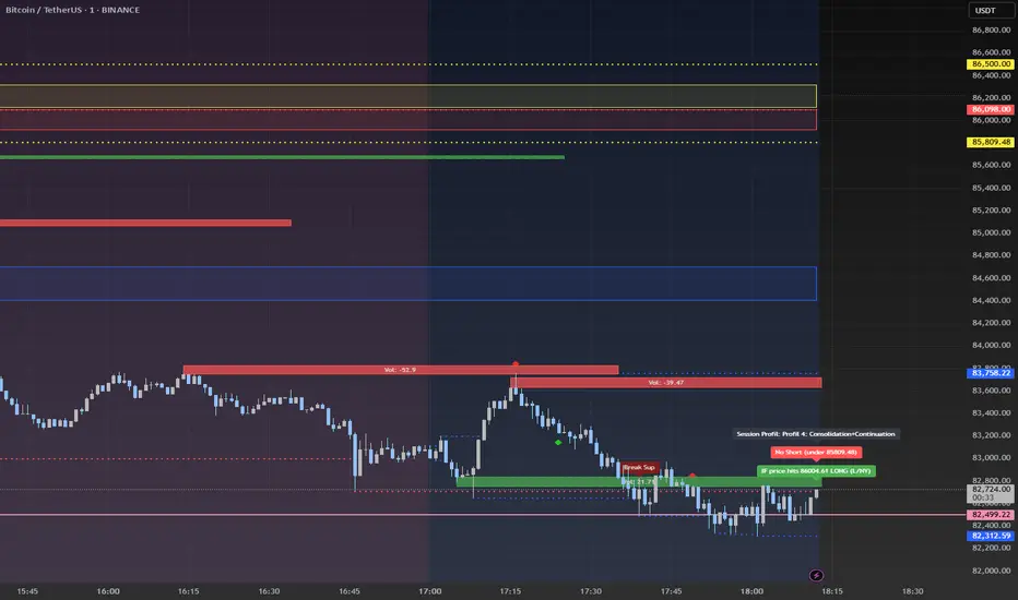
Advanced Session Profile Predictor with SR Boxes & ORAdvanced Session Profile Predictor with Momentum Arrows
Designed for intraday traders, this indicator analyzes price action across Asia, London, and New York sessions to predict market profiles and highlight key trading opportunities. By combining session-based profiling, Opening Range (OR) visualization, and momentum signals from Traders Dynamic Index (TDI), it offers a unique tool for anticipating trends, reversals, and breakouts. Ideal for forex, indices, and crypto on 15M–1H charts.
What Makes This Indicator Unique?
Unlike typical session indicators that only mark time zones or standard TDI scripts that focus on momentum, this tool:
Predicts market profiles (e.g., "Trend Continuation," "NY Manipulation") by analyzing session ranges and directional moves, offering actionable insights into how sessions interact.
Visualizes Opening Range (OR) boxes for the first 15 minutes of each session, helping traders spot early breakout levels.
Integrates TDI with momentum to generate precise bullish/bearish arrows, filtered by session context for improved reliability.
Simplifies decision-making with dynamic profile labels showing real-time long/short conditions based on price levels.
How Does It Work?
Session Tracking:
Asia (00:00–08:00 UTC, yellow), London (08:00–16:00 UTC, red), and New York (13:00–21:00 UTC, blue) sessions are highlighted with background colors and high/low lines (crosses).
OR boxes (first 15 minutes) are drawn for each session: yellow for Asia, red for London, blue for NY.
Profile Prediction:
Compares Asia and London session ranges and directions (e.g., trending if range > 1.5x 5-period SMA).
Examples:
Trend Continuation: Asia and London trend in the same direction—long above Asia high (uptrend) or short below Asia low (downtrend).
NY Manipulation: Asia trends, London consolidates—watch for NY breakouts at London high/low.
Displays the predicted profile and entry conditions in labels (e.g., "IF price hits 1.2000 LONG").
Momentum Arrows:
Uses TDI (RSI period 21, bands 34, fast MA 2) and 12-period momentum.
Green up arrow: Fast MA > upper band (>68) and momentum rising (bullish).
Red down arrow: Fast MA < lower band (<32) and momentum falling (bearish).
Support/Resistance (SR):
Plots dynamic SR boxes based on pivot highs/lows, filtered by volume (inspired by ChartPrime’s methodology, credited below).
How to Use It
Setup: Apply to a 15M–1H chart. Adjust time zone (default: UTC) and session times if needed. Customize TDI/momentum settings for sensitivity.
Trading:
Check the top-right labels for the current profile and entry conditions (e.g., "IF price hits LONG/SHORT").
Confirm entries with green up arrows (bullish) or red down arrows (bearish).
Use OR boxes and session high/low lines to identify breakout or reversal levels.
Example: In "NY Manipulation," wait for price to hit London high (long) or low (short) during NY session, confirmed by an arrow.
Best Markets: Forex (EUR/USD), indices (SPX500), crypto (BTC/USD) with sufficient intraday volatility.
Underlying Concepts
Session Profiling: Detects trends (range > SMA * threshold) and manipulation (e.g., London breaking Asia’s high/low) to predict NY behavior.
OR Boxes: Marks the first 15 minutes’ high/low as a breakout zone (time-based, 900,000 ms).
TDI + Momentum: Combines RSI-based bands with price change (close – close ) for momentum signals.
SR Boxes: Identifies pivots over a lookback period (default 20), scaled by ATR and filtered by volume thresholds.
Credits
The SR box logic is inspired by ChartPrime’s volume-filtered support/resistance methodology, adapted with custom breakout/hold detection. Original authors are credited for their foundational work.
Chart Setup
Displays session backgrounds, OR boxes, high/low lines, TDI arrows, and profile labels. Keep other indicators off for clarity.
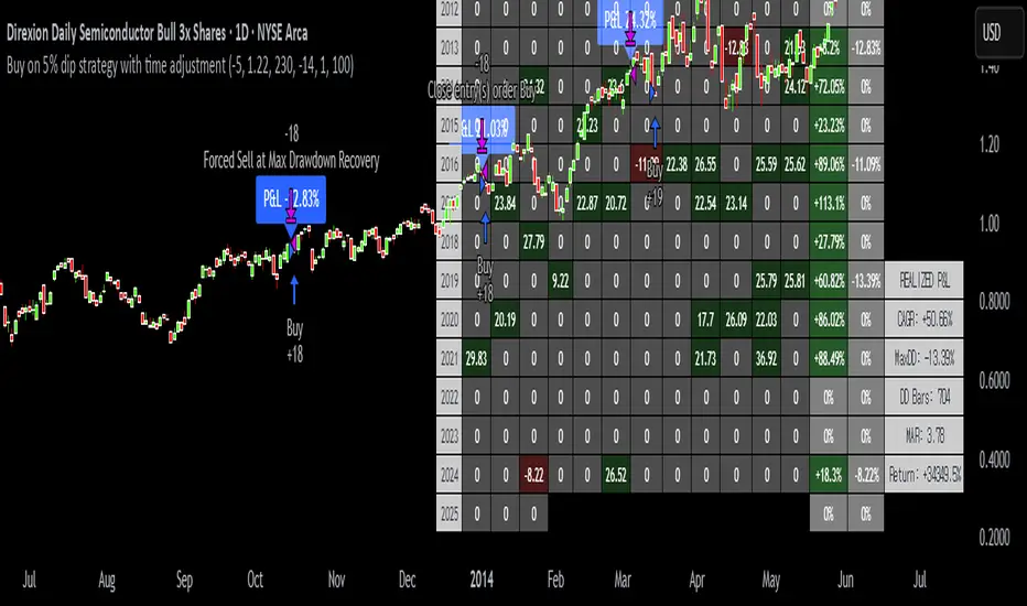
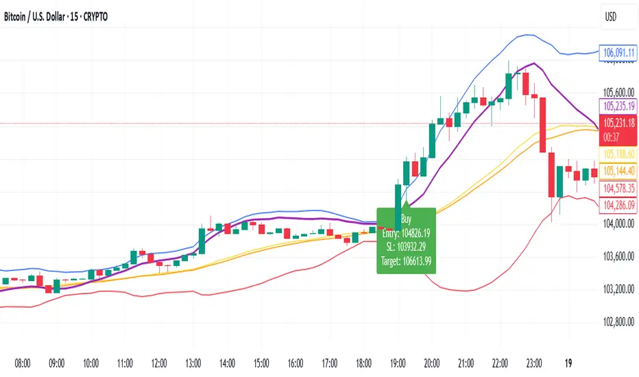
Buy on 5% dip strategy with time adjustment
This script is a strategy called "Buy on 5% Dip Strategy with Time Adjustment 📉💡," which detects a 5% drop in price and triggers a buy signal 🔔. It also automatically closes the position once the set profit target is reached 💰, and it has additional logic to close the position if the loss exceeds 14% after holding for 230 days ⏳.
Strategy Explanation
Buy Condition: A buy signal is triggered when the price drops 5% from the highest price reached 🔻.
Take Profit: The position is closed when the price hits a 1.22x target from the average entry price 📈.
Forced Sell Condition: If the position is held for more than 230 days and the loss exceeds 14%, the position is automatically closed 🚫.
Leverage & Capital Allocation: Leverage is adjustable ⚖️, and you can set the percentage of capital allocated to each trade 💸.
Time Limits: The strategy allows you to set a start and end time ⏰ for trading, making the strategy active only within that specific period.
Code Credits and References
Credits: This script utilizes ideas and code from @QuantNomad and jangdokang for the profit table and algorithm concepts 🔧.
Sources:
Monthly Performance Table Script by QuantNomad:
ZenAndTheArtOfTrading's Script:
Strategy Performance
This strategy provides risk management through take profit and forced sell conditions and includes a performance table 📊 to track monthly and yearly results. You can compare backtest results with real-time performance to evaluate the strategy's effectiveness.
The performance numbers shown in the backtest reflect what would have happened if you had used this strategy since the launch date of the SOXL (the Direxion Daily Semiconductor Bull 3x Shares ETF) 📅. These results are not hypothetical but based on actual performance from the day of the ETF’s launch 📈.
Caution ⚠️
No Guarantee of Future Results: The results are based on historical performance from the launch of the SOXL ETF, but past performance does not guarantee future results. It’s important to approach with caution when applying it to live trading 🔍.
Risk Management: Leverage and capital allocation settings are crucial for managing risk ⚠️. Make sure to adjust these according to your risk tolerance ⚖️.
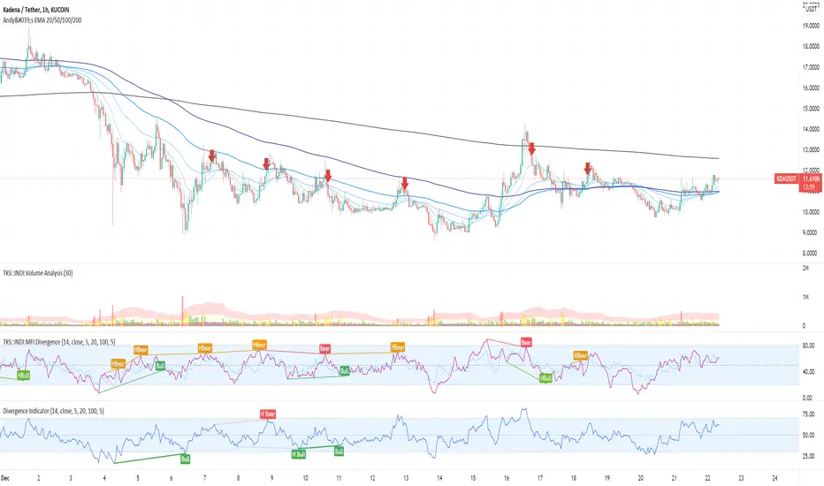
MFI Divergence Indicator Our Developer Malin converted the built-in RSI divergence indicator to MFI (Money Flow Index).
How to apply?
Notice 1: MFI, unlike the RSI, incorporates volume. It thus is an indicator of a higher precision when it comes to finding the the moment to sell - or - the moment to enter.
Notice 2: In Ranging Markets MFI (and RSI) is a solid momentum indicator to buy or sell. The asset displayed shows a slight markdown. Thus, we are looking primarily for short positions. Once can tell by us omitting the first 2 hidden bearish divergence signals and then entering the market.
Notice 3: Divergences depend on pivot points. The drawback with pivot points is that it is a lagging indication of a potential reversal. The more time (bars) one takes to confirm a reversal the less profitable is the trade - but less risky. In the charts one can tell that we enter the market 5 bars later. Usually that is not the tip of the reversal.
Notice 4: One must adapt the left and right periods of the indicator to risk/reward ratio, length of swing / frequency modulation and volatility of the price action.
Credits: Credits go to the Tradingview Team for delivering the original code. And Malin for the conversion. Please keep the copy right as a courtesy.
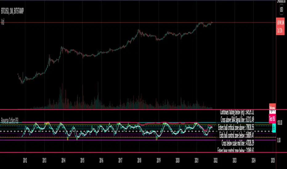
Reverse Cutlers Relative Strength Index On ChartIntroduction
The Reverse Cutlers Relative Strength Index (RCRSI) OC is an indicator which tells the user what price is required to give a particular Cutlers Relative Strength Index ( RSI ) value, or cross its Moving Average (MA) signal line.
Overview
Background & Credits:
The relative strength index ( RSI ) is a momentum indicator used in technical analysis that was originally developed by J. Welles Wilder Jr. and introduced in his seminal 1978 book, “New Concepts in Technical Trading Systems.”.
Cutler created a variation of the RSI known as “Cutlers RSI” using a different formulation to avoid an inherent accuracy problem which arises when using Wilders method of smoothing.
Further developments in the use, and more nuanced interpretations of the RSI have been developed by Cardwell, and also by well-known chartered market technician, Constance Brown C.M.T., in her acclaimed book "Technical Analysis for the Trading Professional” 1999 where she described the idea of bull and bear market ranges for RSI , and while she did not actually reveal the formulas, she introduced the concept of “reverse engineering” the RSI to give price level outputs.
Renowned financial software developer, co-author of academic books on finance, and scientific fellow to the Department of Finance and Insurance at the Technological Educational Institute of Crete, Giorgos Siligardos PHD . brought a new perspective to Wilder’s RSI when he published his excellent and well-received articles "Reverse Engineering RSI " and "Reverse Engineering RSI II " in the June 2003, and August 2003 issues of Stocks & Commodities magazine, where he described his methods of reverse engineering Wilders RSI .
Several excellent Implementations of the Reverse Wilders Relative Strength Index have been published here on Tradingview and elsewhere.
My utmost respect, and all due credits to authors of related prior works.
Introduction
It is worth noting that while the general RSI formula, and the logic dictating the UpMove and DownMove data series has remained the same as the Wilders original formulation, it has been interpreted in a different way by using a different method of averaging the upward, and downward moves.
Cutler recognized the issue of data length dependency when using wilders smoothing method of calculating RSI which means that wilders standard RSI will have a potential initialization error which reduces with every new data point calculated meaning early results should be regarded as unreliable until enough calculation iterations have occurred for convergence.
Hence Cutler proposed using Simple Moving Averaging for gain and loss data which this Indicator is based on.
Having "Reverse engineered" prices for any oscillator makes the planning, and execution of strategies around that oscillator far simpler, more timely and effective.
Introducing the Reverse Cutlers RSI which consists of plotted lines on a scale of 0 to 100, and an optional infobox.
The RSI scale is divided into zones:
• Scale high (100)
• Bull critical zone (80 - 100)
• Bull control zone (62 - 80)
• Scale midline (50)
• Bear control zone (20 - 38)
• Bear critical zone (0 - 20)
• Scale low (0)
The RSI plots which graphically display output closing price levels where Cutlers RSI value will crossover:
• RSI (eq) (previous RSI value)
• RSI MA signal line
• RSI Test price
• Alert level high
• Alert level low
The info box displays output closing price levels where Cutlers RSI value will crossover:
• Its previous value. ( RSI )
• Bull critical zone.
• Bull control zone.
• Mid-Line.
• Bear control zone.
• Bear critical zone.
• RSI MA signal line
• Alert level High
• Alert level low
And also displays the resultant RSI for a user defined closing price:
• Test price RSI
The infobox outputs can be shown for the current bar close, or the next bar close.
The user can easily select which information they want in the infobox from the setttings
Importantly:
All info box price levels for the current bar are calculated immediately upon the current bar closing and a new bar opening, they will not change until the current bar closes.
All info box price levels for the next bar are projections which are continually recalculated as the current price changes, and therefore fluctuate as the current price changes.
Understanding the Relative Strength Index
At its simplest the RSI is a measure of how quickly traders are bidding the price of an asset up or down.
It does this by calculating the difference in magnitude of price gains and losses over a specific lookback period to evaluate market conditions.
The RSI is displayed as an oscillator (a line graph that can move between two extremes) and outputs a value limited between 0 and 100.
It is typically accompanied by a moving average signal line.
Traditional interpretations
Overbought and oversold:
An RSI value of 70 or above indicates that an asset is becoming overbought (overvalued condition), and may be may be ready for a trend reversal or corrective pullback in price.
An RSI value of 30 or below indicates that an asset is becoming oversold (undervalued condition), and may be may be primed for a trend reversal or corrective pullback in price.
Midline Crossovers:
When the RSI crosses above its midline ( RSI > 50%) a bullish bias signal is generated. (only take long trades)
When the RSI crosses below its midline ( RSI < 50%) a bearish bias signal is generated. (only take short trades)
Bullish and bearish moving average signal Line crossovers:
When the RSI line crosses above its signal line, a bullish buy signal is generated
When the RSI line crosses below its signal line, a bearish sell signal is generated.
Swing Failures and classic rejection patterns:
If the RSI makes a lower high, and then follows with a downside move below the previous low, a Top Swing Failure has occurred.
If the RSI makes a higher low, and then follows with an upside move above the previous high, a Bottom Swing Failure has occurred.
Examples of classic swing rejection patterns
Bullish swing rejection pattern:
The RSI moves into oversold zone (below 30%).
The RSI rejects back out of the oversold zone (above 30%)
The RSI forms another dip without crossing back into oversold zone.
The RSI then continues the bounce to break up above the previous high.
Bearish swing rejection pattern:
The RSI moves into overbought zone (above 70%).
The RSI rejects back out of the overbought zone (below 70%)
The RSI forms another peak without crossing back into overbought zone.
The RSI then continues to break down below the previous low.
Divergences:
A regular bullish RSI divergence is when the price makes lower lows in a downtrend and the RSI indicator makes higher lows.
A regular bearish RSI divergence is when the price makes higher highs in an uptrend and the RSI indicator makes lower highs.
A hidden bullish RSI divergence is when the price makes higher lows in an uptrend and the RSI indicator makes lower lows.
A hidden bearish RSI divergence is when the price makes lower highs in a downtrend and the RSI indicator makes higher highs.
Regular divergences can signal a reversal of the trending direction.
Hidden divergences can signal a continuation in the direction of the trend.
Chart Patterns:
RSI regularly forms classic chart patterns that may not show on the underlying price chart, such as ascending and descending triangles & wedges , double tops, bottoms and trend lines etc.
Support and Resistance:
It is very often easier to define support or resistance levels on the RSI itself rather than the price chart.
Modern interpretations in trending markets:
Modern interpretations of the RSI stress the context of the greater trend when using RSI signals such as crossovers, overbought/oversold conditions, divergences and patterns.
Constance Brown, CMT , was one of the first who promoted the idea that an oversold reading on the RSI in an uptrend is likely much higher than 30%, and that an overbought reading on the RSI during a downtrend is much lower than the 70% level.
In an uptrend or bull market, the RSI tends to remain in the 40 to 90 range, with the 40-50 zone acting as support.
During a downtrend or bear market, the RSI tends to stay between the 10 to 60 range, with the 50-60 zone acting as resistance.
For ease of executing more modern and nuanced interpretations of RSI it is very useful to break the RSI scale into bull and bear control and critical zones.
These ranges will vary depending on the RSI settings and the strength of the specific market’s underlying trend.
Limitations of the RSI
Like most technical indicators, its signals are most reliable when they conform to the long-term trend.
True trend reversal signals are rare, and can be difficult to separate from false signals.
False signals or “fake-outs”, e.g. a bullish crossover, followed by a sudden decline in price, are common.
Since the indicator displays momentum, it can stay overbought or oversold for a long time when an asset has significant sustained momentum in either direction.
Data Length Dependency when using wilders smoothing method of calculating RSI means that wilders standard RSI will have a potential initialization error which reduces with every new data point calculated meaning early results should be regarded as unreliable until calculation iterations have occurred for convergence.

Reverse Cutlers Relative Strength IndexIntroduction
The Reverse Cutlers Relative Strength Index (RCRSI) is an indicator which tells the user what price is required to give a particular Cutlers Relative Strength Index (RSI) value, or cross its Moving Average (MA) signal line.
Overview
Background & Credits:
The relative strength index (RSI) is a momentum indicator used in technical analysis that was originally developed by J. Welles Wilder Jr. and introduced in his seminal 1978 book, “New Concepts in Technical Trading Systems.”.
Cutler created a variation of the RSI known as “Cutlers RSI” using a different formulation to avoid an inherent accuracy problem which arises when using Wilders method of smoothing.
Further developments in the use, and more nuanced interpretations of the RSI have been developed by Cardwell, and also by well-known chartered market technician, Constance Brown C.M.T., in her acclaimed book "Technical Analysis for the Trading Professional” 1999 where she described the idea of bull and bear market ranges for RSI, and while she did not actually reveal the formulas, she introduced the concept of “reverse engineering” the RSI to give price level outputs.
Renowned financial software developer, co-author of academic books on finance, and scientific fellow to the Department of Finance and Insurance at the Technological Educational Institute of Crete, Giorgos Siligardos PHD. brought a new perspective to Wilder’s RSI when he published his excellent and well-received articles "Reverse Engineering RSI " and "Reverse Engineering RSI II " in the June 2003, and August 2003 issues of Stocks & Commodities magazine, where he described his methods of reverse engineering Wilders RSI.
Several excellent Implementations of the Reverse Wilders Relative Strength Index have been published here on Tradingview and elsewhere.
My utmost respect, and all due credits to authors of related prior works.
Introduction
It is worth noting that while the general RSI formula, and the logic dictating the UpMove and DownMove data series as described above has remained the same as the Wilders original formulation, it has been interpreted in a different way by using a different method of averaging the upward, and downward moves.
Cutler recognized the issue of data length dependency when using wilders smoothing method of calculating RSI which means that wilders standard RSI will have a potential initialization error which reduces with every new data point calculated meaning early results should be regarded as unreliable until enough calculation iterations have occurred for convergence.
Hence Cutler proposed using Simple Moving Averaging for gain and loss data which this Indicator is based on.
Having "Reverse engineered" prices for any oscillator makes the planning, and execution of strategies around that oscillator far simpler, more timely and effective.
Introducing the Reverse Cutlers RSI which consists of plotted lines on a scale of 0 to 100, and an optional infobox.
The RSI scale is divided into zones:
• Scale high (100)
• Bull critical zone (80 - 100)
• Bull control zone (62 - 80)
• Scale midline (50)
• Bear critical zone (20 - 38)
• Bear control zone (0 - 20)
• Scale low (0)
The RSI plots are:
• Cutlers RSI
• RSI MA signal line
• Test price RSI
• Alert level high
• Alert level low
The info box displays output closing price levels where Cutlers RSI value will crossover:
• Its previous value. (RSI )
• Bull critical zone.
• Bull control zone.
• Mid-Line.
• Bear control zone.
• Bear critical zone.
• RSI MA signal line
• Alert level High
• Alert level low
And also displays the resultant RSI for a user defined closing price:
• Test price RSI
The infobox outputs can be shown for the current bar close, or the next bar close.
The user can easily select which information they want in the infobox from the setttings
Importantly:
All info box price levels for the current bar are calculated immediately upon the current bar closing and a new bar opening, they will not change until the current bar closes.
All info box price levels for the next bar are projections which are continually recalculated as the current price changes, and therefore fluctuate as the current price changes.
Understanding the Relative Strength Index
At its simplest the RSI is a measure of how quickly traders are bidding the price of an asset up or down.
It does this by calculating the difference in magnitude of price gains and losses over a specific lookback period to evaluate market conditions.
The RSI is displayed as an oscillator (a line graph that can move between two extremes) and outputs a value limited between 0 and 100.
It is typically accompanied by a moving average signal line.
Traditional interpretations
Overbought and oversold:
An RSI value of 70 or above indicates that an asset is becoming overbought (overvalued condition), and may be may be ready for a trend reversal or corrective pullback in price.
An RSI value of 30 or below indicates that an asset is becoming oversold (undervalued condition), and may be may be primed for a trend reversal or corrective pullback in price.
Midline Crossovers:
When the RSI crosses above its midline (RSI > 50%) a bullish bias signal is generated. (only take long trades)
When the RSI crosses below its midline (RSI < 50%) a bearish bias signal is generated. (only take short trades)
Bullish and bearish moving average signal Line crossovers:
When the RSI line crosses above its signal line, a bullish buy signal is generated
When the RSI line crosses below its signal line, a bearish sell signal is generated.
Swing Failures and classic rejection patterns:
If the RSI makes a lower high, and then follows with a downside move below the previous low, a Top Swing Failure has occurred.
If the RSI makes a higher low, and then follows with an upside move above the previous high, a Bottom Swing Failure has occurred.
Examples of classic swing rejection patterns
Bullish swing rejection pattern:
The RSI moves into oversold zone (below 30%).
The RSI rejects back out of the oversold zone (above 30%)
The RSI forms another dip without crossing back into oversold zone.
The RSI then continues the bounce to break up above the previous high.
Bearish swing rejection pattern:
The RSI moves into overbought zone (above 70%).
The RSI rejects back out of the overbought zone (below 70%)
The RSI forms another peak without crossing back into overbought zone.
The RSI then continues to break down below the previous low.
Divergences:
A regular bullish RSI divergence is when the price makes lower lows in a downtrend and the RSI indicator makes higher lows.
A regular bearish RSI divergence is when the price makes higher highs in an uptrend and the RSI indicator makes lower highs.
A hidden bullish RSI divergence is when the price makes higher lows in an uptrend and the RSI indicator makes lower lows.
A hidden bearish RSI divergence is when the price makes lower highs in a downtrend and the RSI indicator makes higher highs.
Regular divergences can signal a reversal of the trending direction.
Hidden divergences can signal a continuation in the direction of the trend.
Chart Patterns:
RSI regularly forms classic chart patterns that may not show on the underlying price chart, such as ascending and descending triangles & wedges, double tops, bottoms and trend lines etc.
Support and Resistance:
It is very often easier to define support or resistance levels on the RSI itself rather than the price chart.
Modern interpretations in trending markets:
Modern interpretations of the RSI stress the context of the greater trend when using RSI signals such as crossovers, overbought/oversold conditions, divergences and patterns.
Constance Brown, CMT, was one of the first who promoted the idea that an oversold reading on the RSI in an uptrend is likely much higher than 30%, and that an overbought reading on the RSI during a downtrend is much lower than the 70% level.
In an uptrend or bull market, the RSI tends to remain in the 40 to 90 range, with the 40-50 zone acting as support.
During a downtrend or bear market, the RSI tends to stay between the 10 to 60 range, with the 50-60 zone acting as resistance.
For ease of executing more modern and nuanced interpretations of RSI it is very useful to break the RSI scale into bull and bear control and critical zones.
These ranges will vary depending on the RSI settings and the strength of the specific market’s underlying trend.
Limitations of the RSI
Like most technical indicators, its signals are most reliable when they conform to the long-term trend.
True trend reversal signals are rare, and can be difficult to separate from false signals.
False signals or “fake-outs”, e.g. a bullish crossover, followed by a sudden decline in price, are common.
Since the indicator displays momentum, it can stay overbought or oversold for a long time when an asset has significant sustained momentum in either direction.
Data Length Dependency when using wilders smoothing method of calculating RSI means that wilders standard RSI will have a potential initialization error which reduces with every new data point calculated meaning early results should be regarded as unreliable until calculation iterations have occurred for convergence.
ATR Start & Stop BotThis script is using Average True Range (ATR) and works very well on the Bitcoin 4 hour timeframe to determine when to stop and start your bots.
It has a very similar visual to the EMA RSI Indicator found here:
This 'ATR Start & Stop Bot' is better because it has less confusion during sideways market movement.
As an example - You are using 3commas and have a Composite bot setup with several alt coins, you can use this indicator with the ' Stop bot ' alert to disable your composite bot from taking trades at times when the market is on a trend that looks in the red.
Alternatively you can use the ' Start bot ' alert to turn your bot back on during the green uptrends.
Using this indicator with these alerts on the Bitcoin 4-Hour chart add a great layer of automation to your already existing bots.
Credits:
Original 'ATR Stops' indicator belong to the user failathon and that script is found here:
Also credits to Dradian for the alert additions.

Bollinger Band StrategyDescription of the Bollinger Band Breakout Strategy
This trading strategy, credited to Siddhart Bhanushali, is a momentum-based approach that uses Bollinger Bands and a 22-period Simple Moving Average (SMA) to identify high-probability breakout trades. It focuses on detecting periods of low volatility (contraction) followed by high volatility (expansion) to enter trades with a favorable risk-reward ratio. The strategy is designed to capture significant price movements in trending markets, with clear rules for entry, stop loss, and profit targets.
Strategy Overview
The strategy generates buy and sell signals based on specific conditions involving the 22-period SMA and Bollinger Bands. It aims to enter trades when the price breaks out of a consolidation phase, confirmed by the direction of the SMA and the behavior of a green or red candle relative to the Bollinger Bands. The minimum target for each trade is a 1:2 risk-reward ratio.
Credit
This strategy is credited to Siddhart Bhanushali, who designed it to leverage Bollinger Band breakouts in trending markets, providing a clear and systematic approach to trading with defined risk-reward parameters.
7 EMA CloudThe "7 EMA Cloud" script was likely flagged because it reuses the core concept of EMA clouds (shading areas between multiple EMAs to visualize trends, support/resistance, and momentum) without crediting the original inventor, Ripster (author ripster47 on TradingView). This concept is prominently associated with Ripster's "EMA Clouds" indicator, which popularized filling spaces between EMA pairs for trading signals. TradingView's house rules require crediting authors when reusing open-source ideas or code, even if not a direct copy-paste, and mandate significant improvements where the original forms a small proportion of the script. Your version adds features like multiple color modes (Classic rainbow, Monochrome, Heatmap), customizable signal sizes, and crossover alerts between the first and last EMA, which are enhancements, but the foundational EMA ribbon/cloud idea needs explicit attribution in the description and ideally code comments to comply.
Additionally, the description might be seen as not fully self-contained (e.g., it uses promotional language like "Advanced" and "Adaptive Trend & Signal Suite" without deeply explaining calculations or use cases), potentially violating rules against relying on code or external references for clarity.
To fix this, republish a new version with proper credits, ensure the description is detailed and standalone, and emphasize your improvements (e.g., the 7 Fibonacci-based EMAs, color modes, and signals). Do not reuse the flagged script—create a fresh one. Here's a compliant description you can use:
7 EMA Cloud Indicator
Overview
The 7 EMA Cloud overlays seven exponential moving averages (EMAs) with Fibonacci-inspired periods and fills the spaces between them with customizable "clouds" to visually represent trend strength, direction, and convergence/divergence. It includes crossover signals between the shortest and longest EMAs for potential entry/exit points, with adjustable visual modes for different trading styles. This helps traders identify bullish/bearish momentum, support/resistance zones, and overextensions in trending or ranging markets.
This script builds on the EMA cloud concept popularized by Ripster (ripster47) in their "EMA Clouds" indicatortradingview.com, where areas between EMA pairs are shaded for trend analysis. Improvements include a fixed set of 7 Fibonacci EMAs, multiple color schemes (Classic rainbow, Monochrome grayscale, Heatmap for intensity), user-selectable signal sizes, and transparency controls. Released under the Mozilla Public License 2.0.
Key Features
7 EMAs with Clouds: EMAs at periods 8, 13, 21, 34, 55, 89, and 144; clouds filled between consecutive pairs to show alignment (tight clouds for consolidation, wide for trends).
Color Modes:
Classic: Rainbow gradients (blue to purple) for vibrant distinction.
Monochrome: Grayscale shades for minimalistic charts.
Heatmap: Red-to-blue spectrum to highlight "hot" (volatile) vs. "cool" (stable) areas.
Crossover Signals: Triangle markers (up for bullish, down for bearish) when the shortest EMA crosses the longest; sizes from Tiny to Huge.
Display Options: Toggle EMA lines on/off, adjust cloud transparency (0-100%), and enable alerts for crossovers.
Alerts: Notifications for "Bullish EMA Crossover" (EMA1 > EMA7) and "Bearish EMA Crossover" (EMA1 < EMA7).
How It Works
EMA Calculations: Each EMA is computed using ta.ema(close, period), with periods based on Fibonacci sequences for natural market rhythm alignment.
Clouds: Filled via fill() between plot pairs, with colors derived from the selected mode and transparency applied.
Signals: Detected with ta.crossover(ema1, ema7) and ta.crossunder(ema1, ema7), plotted as shapes with mode-specific colors (e.g., green/lime for bull, red for bear).
Customization: Inputs grouped into EMA Settings (periods), Display Settings (visibility, colors, transparency), and Signal Settings (size).
Customization Options
EMA Periods: Individually adjustable (defaults: 8, 13, 21, 34, 55, 89, 144).
Show EMAs: Toggle to hide lines and focus on clouds.
Cloud Transparency: 0% for solid fills, 100% for invisible (default 80%).
Color Mode: Switch between Classic, Monochrome, or Heatmap.
Signal Size: Tiny, Small, Normal, Large, or Huge for crossover markers.
Ideal Use Case
Suited for swing or trend-following on any timeframe (e.g., 15m-1h for intraday, daily for swings) and assets (stocks, forex, crypto, futures). Enter long on bullish crossovers above aligned clouds; exit on bearish signals or cloud widenings. Use Monochrome for clean charts or Heatmap for volatility emphasis. Combine with volume or RSI for confirmation.
Why It's Valuable
By expanding Ripster's EMA cloud idea with multi-mode visuals and integrated signals, this indicator provides a versatile, at-a-glance tool for trend assessment—reducing noise while highlighting key shifts. It's more adaptive than basic MA ribbons, with Fibonacci periods adding a layer of harmonic analysis.
Note: Test on historical data or demo accounts. Not financial advice—incorporate risk management. Optimized for Pine Script v5; some features may vary on non-overlay charts.

Candlestick Patterns Backtester [Optimized]Candlestick Patterns Backtester
What this is: This indicator is based on a really cool candlestick pattern backtester that I found (I'll update this later when I remember where I got it from or find the actual author). The original had this massive table showing win/loss ratios for a bunch of candlestick patterns, and according to the built-in backtester, it was actually profitable - which was pretty impressive.
The Problem: I played around with the original for a while but honestly wasn't really able to get it to work well at all for actual trading. It was still pretty cool to look at though! The main issues were:
It was just a big static table - hard to do anything useful with it
Couldn't send signals out to other strategies
The code was a monster - like 2,000+ lines of repetitive mess
What I Did: I completely refactored this thing and got it down from 2,000+ lines to just a few hundred lines. Much cleaner now! Here's what it does:
45+ Candlestick Patterns - All the classics are in there
Dynamic Filtering - Set your own requirements (minimum win rate, profit factor, total trades, etc.)
Flexible Logic - Choose AND/OR logic for your filters
Signal Generation - Creates actual buy/sell signals you can use with other strategies
Visual Badges - Shows pattern badges on chart when they meet your criteria
Active Patterns Table - Only shows patterns that are currently profitable based on your settings
Settings You Can Adjust:
Minimum win rate threshold
Minimum profit factor
Minimum number of trades required
Whether to use AND or OR logic for filtering
Colors, badge display, debug options
Reality Check: Trading these patterns really wasn't for me, but it was still a great learning experience. The backtesting results look good on paper, but as always, past performance doesn't guarantee future results. Use this as a research tool and educational resource more than anything else.
Credit: This is based on someone else's original work that I heavily modified and optimized. I'll update this description once I track down the original author to give proper credit where it's due.
This introduction captures your casual, honest tone while explaining the technical improvements you made and setting realistic expectations about the indicator's practical use.
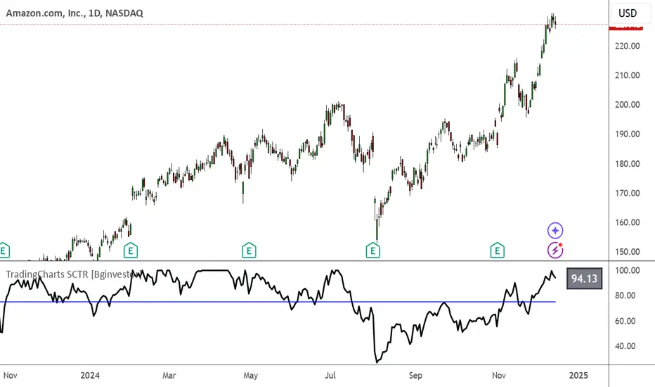
TradingCharts SCTR [Bginvestor]This indicator is replicating Tradingcharts, SCTR plot. If you know, you know.
Brief description: The StockCharts Technical Rank (SCTR), conceived by technical analyst John Murphy, emerges as a pivotal tool in evaluating a stock’s technical prowess. This numerical system, colloquially known as “scooter,” gauges a stock’s strength within various groups, employing six key technical indicators across different time frames.
How to use it:
Long-term indicators (30% weight each)
-Percent above/below the 200-day exponential moving average (EMA)
-125-day rate-of-change (ROC)
Medium-term indicators (15% weight each)
-percent above/below 50-day EMA
-20-day rate-of-change
Short-term indicators (5% weight each)
-Three-day slope of percentage price oscillator histogram divided by three
-Relative strength index
How to use SCTR:
Investors select a specific group for analysis, and the SCTR assigns rankings within that group. A score of 99.99 denotes robust technical performance, while zero signals pronounced underperformance. Traders leverage this data for strategic decision-making, identifying stocks with increasing SCTR for potential buying or spotting weak stocks for potential shorting.
Credit: I've made some modifications, but credit goes to GodziBear for back engineering the averaging / scaling of the equations.
Note: Not a perfect match to TradingCharts, but very, very close.
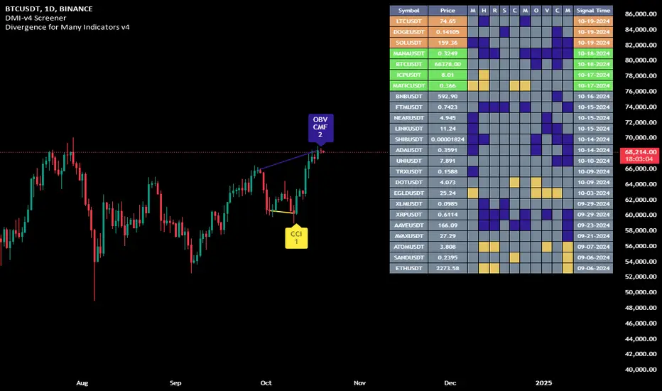
Divergence for Many Indicators v4 Screener▋ INTRODUCTION:
The “Divergence for Many Indicators v4 Screener” is developed to provide an advanced monitoring solution for up to 24 symbols simultaneously. It efficiently collects signals from multiple symbols based on the “ Divergence for Many Indicators v4 ” and presents the output in an organized table. The table includes essential details starting with the symbol name, signal price, corresponding divergence indicator, and signal time.
_______________________
▋ CREDIT:
The divergence formula adapted from the “ Divergence for Many Indicators v4 ” script, originally created by @LonesomeTheBlue . Full credit to his work.
_______________________
▋ OVERVIEW:
The chart image can be considered an example of a recorded divergence signal that occurred in $BTCUSDT.
_______________________
▋ APPEARANCE:
The table can be displayed in three formats:
1. Full indicator name.
2. First letter of the indicator name.
3. Total number of divergences.
_______________________
▋ SIGNAL CONFIRMATION:
The table distinguishes signal confirmation by using three different colors:
1. Not-Confirmed (Orange): The signal is not confirmed yet, as the bar is still open.
2. Freshly Confirmed (Green): The signal was confirmed 1 or 2 bars ago.
3. Confirmed (Gray): The signal was confirmed 3 or more bars ago.
_______________________
▋ INDICATOR SETTINGS:
Section(1): Table Settings
(1) Table location on the chart.
(2) Table’s cells size.
(3) Chart’s timezone.
(4) Sorting table.
- Signal: Sorts the table by the latest signals.
- None: Sorts the table based on the input order.
(5) Table’s colors.
(6) Signal Confirmation type color. Explained above in the SIGNAL CONFIRMATION section
Section(2): Divergence for Many Indicators v4 Settings
As seen on the Divergence for Many Indicators v4
* Explained above in the APPEARANCE section
Section(3): Symbols
(1) Enable/disable symbol in the screener.
(2) Entering a symbol.
_______________________
▋ FINAL COMMENTS:
For best performance, add the Screener indicator to an active symbol chart, such as QQQ, SPY, AAPL, BTCUSDT, ES, EURUSD, etc., and avoid mixing symbols from different market allocations.
The Divergence for Many Indicators v4 Screener indicator is not a primary tool for making trading decisions.
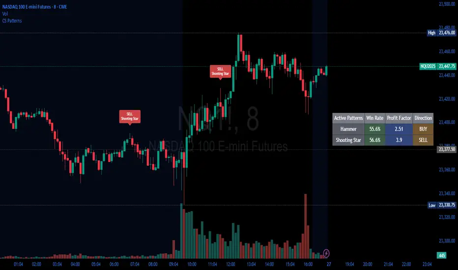
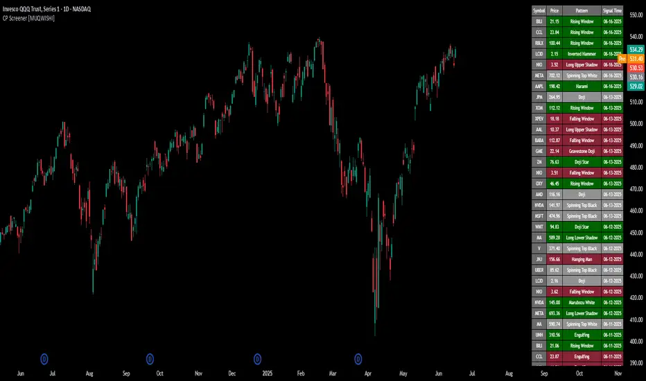
All Candlestick Patterns on Backtest [By MUQWISHI]▋ INTRODUCTION :
The “All Candlestick Patterns on Backtest” indicator generates a table that offers a clear visualization of the historical return percentages for each candlestick pattern strategy over a specified time period. This table serves as an organized resource, serving as a launching point for in-depth research into candle formations. It may help to rectify any misconceptions surrounding candlestick patterns, refine trading approaches, and it could be foundation to make informed decisions in trading journey.
_______________________
▋ OVERVIEW:
_______________________
▋ CREDIT:
Credit to public technical “*All Candlestick Patterns*” indicator.
_______________________
▋ TABLE:
_______________________
▋ CHART:
_______________________
▋ INDICATOR SETTINGS:
#Section One: Table Setting
#Section Two: Backtest Setting
(1) Backtest Starting Period.
Note: If the datetime of the first candle on the chart is after the entreated datetime, the calculation will start from the first candle on the chart.
(2) Initial Equity ($).
(3) Leverage: Current Equity x Leverage Value.
(4) Entry Mode:
- “At Close”: Execute entry order as soon as the candle confirmed.
- “Breakout High (Low for Short)”: Stop limit buy order, entry order will be executed as soon as the next candle breakout the high of last pattern’s candle (low for short)
(5) Cancel Entry Within Bars: This option is applicable with {Entry Mode = Breakout High (Low for Short)}, to cancel the Entry Order if it's not executed within certain selected number of bars.
(6) Stoploss Range: the range refers to high of pattern - low of pattern.
(7) Risk:Reward: the calculation of risk:reward range start from entry price level. For example: A pattern triggered with range 10 points, and entry price is 100.
- For 1:1~risk:reward would the stoploss at 90 and takeprofit at 110.
- For 1:3~risk:reward would the stoploss at 90 and takeprofit at 130.
#Section Three: Technical & Candle Patterns
_______________________
▋ Comments:
This table was developed for research and educational purposes.
Candlestick patterns are almost similar as seen in “*All Candlestick Patterns*” indicator.
The table results should not be taken as a major concept to build a trading decision.
Personally, I see candlestick patterns as a means to comprehend the psychology of the market, and help to follow the price action.
Please let me know if you have any questions.
Thank you.

All Candlestick Patterns Screener [By MUQWISHI]▋ INTRODUCTION :
The Candlestick Patterns Screener has been designed to offer an advanced monitoring solution for up to 40 symbols. Utilizing a log screener style, it efficiently gathers information on confirmed candlestick pattern occurrences and presents it in an organized table. This table includes essential details such as the symbol name, signal price, and the corresponding candlestick pattern name.
_______________________
▋ OVERVIEW:
_______________________
▋ CREDIT:
Credit to public technical “*All Candlestick Patterns*” indicator.
_______________________
▋ USAGE:
_______________________
▋ Final Comments:
For best performance, add the Candlestick Patterns Screener on active symbol chart like QQQ, SPY, AAPL, BTCUSDT, ES, EURUSD or …etc.
Candlestick patterns are not a major concept to build a trading decision.
Personally, I see candlestick patterns as a means to comprehend the psychology of the market, and help to follow the price action.
Please let me know if you have any questions.
Thank you.
Funding Rate for FTX:BTCPERP (estimated) v0.1 Original credits goes to @Hayemaker, and @NeoButane for the TWAP portions of this script
By @davewhiiite, 2021-03-27
Version 0.1
Summary: The funding rate is the interest charged / credited to a perpetual futures trader for taking a long or short position. The direction of the funding rate is used as an indicator of trader sentiment (+ve = bullish; -ve = bearish), and therefore useful to plot in real time.
The FTX exchange has published the calculation of their funding rate as follows:
TWAP((future - index) / index) / 24
The formula here is the same, but expresses it in the more common % per 8hr duration:
funding = TWAP((future / index) - 1) * (8 / 24) * 100
For reference: future refers to the FTX bitcoin futures contract price (FTX:BTCPERP) and index is the spot price of bitcoin on the exchange (FTX:BTCUSD)
Additional notes:
Probably best to add to the indicator to a new pane, or as secondary axis
Plot this in combination with FTX:BTCPERP or FTX:BTCUSD, or chart of your choice to complement your bitcoin dashboard
Compare to funding rates published on ViewBase
questions? Ask me!
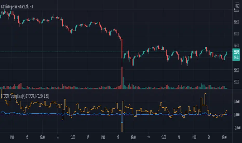
Price Persistence ScreenerPrice Persistence Screener
Pine Script v6 | Inspired by @pradeepbonde on X
This indicator, inspired by the insights of @pradeepbonde , is designed to identify stocks with high price persistence—stocks that consistently close higher than the previous day's close over various lookback periods. As described by Pradeep Bonde, stocks with high persistence are strong candidates for trading pullbacks or consolidations, as they often resume their upward trend due to aggressive buying and low selling pressure. This tool helps traders screen for such stocks and visualize their persistence across multiple timeframes.
Features:
Measures price persistence by counting bars where the closing price exceeds the previous bar’s close for fixed periods: 499, 252, 126, 60, 40, 20, 15, 10, and 5 bars.
Includes a customizable lookback period (1 to 499 bars) for flexible analysis.
Allows users to set a custom persistence threshold (0% to 100%) to highlight strong bullish trends.
How It Works:
For each lookback period, the indicator calculates how many times the closing price is higher than the previous bar’s close.
A higher count indicates stronger bullish persistence, signaling stocks with sustained upward momentum.
Usage:
This screener is aimed to be used on pine screener to see data in columns. Add this indicator to you favorites and in pine screener scan on your watchlist of up to 1000 stocks
Adjust the custom lookback period and threshold via input settings.
Sort columns to compare persistence across timeframes and identify stocks with high persistence for swing trading or long-term holding.
Settings:
Custom Lookback Period (Bars): Set the number of bars for the custom persistence calculation (default: 100).
Custom Persistence Threshold (%): Define the percentage threshold for highlighting high persistence in the custom period (default: 70%).
Credits:
This indicator is based on the price persistence concept shared by @pradeepbonde
in his YouTube video (www.youtube.com). He explains that stocks with high persistence—those consistently closing higher day after day—are strong candidates for trading pullbacks, as they tend to resume their upward trend. This screener automates and visualizes that concept, making it easier for traders to identify such stocks.
Note:
Ensure sufficient historical data is available for accurate calculations, especially for longer periods like 499 bars. if stock is less than 499 bars.
High persistence stocks may eventually lose momentum, signaling potential reversals or shorting opportunities, as noted by @pradeepbonde
.
Use this indicator as part of a broader trading strategy to screen strong trends with custom lookback scan, combining it with other technical or fundamental analysis.

Grand Master's Candlestick Dominance (ATR Enhanced)### Grand Master's Candlestick Dominance (ATR Enhanced)
**Overview**
Unleash the ancient wisdom of Japanese candlestick charting with a modern twist! This comprehensive Pine Script v5 strategy and indicator scans for over 75 classic and advanced candlestick patterns (bullish, bearish, and neutral), assigning dynamic strength scores (1-10) to each for precise signal filtering. Enhanced with Average True Range (ATR) for volatility-aware body size validation, it dominates the markets by combining timeless pattern recognition with robust confirmation layers. Whether used as a backtestable strategy or visual indicator, it empowers traders to spot high-probability reversals, continuations, and indecision setups with surgical accuracy.
Inspired by Steve Nison's *Japanese Candlestick Charting Techniques*, this tool elevates pattern analysis beyond basics—think Hammers, Engulfing patterns, Morning Stars, and rare gems like Abandoned Baby or Concealing Baby Swallow—all consolidated into intelligent arrays for real-time averaging and prioritization.
**Key Features**
- **Extensive Pattern Library**:
- **Bullish (25+ patterns)**: Hammer (8.0), Bullish Engulfing (10.0), Morning Star (7.0), Three White Soldiers (9.0), Dragonfly Doji (8.0), and more (e.g., Rising Three, Unique Three River Bottom).
- **Bearish (25+ patterns)**: Hanging Man (8.0), Bearish Engulfing (10.0), Evening Star (7.0), Three Black Crows (9.0), Gravestone Doji (8.0), and exotics like Upside Gap Two Crows or Stalled Pattern.
- **Neutral/Indecision (34+ patterns)**: Doji variants (Long-Legged, Four Price), Spinning Tops, Harami Crosses, and multi-bar setups like Upside Tasuki Gap or Advancing Block.
Each pattern includes duration tracking (1-5 bars) and ATR-adjusted body/shadow criteria for relevance in volatile conditions.
- **Smart Confirmation Filters** (All Toggleable):
- **Trend Alignment**: 20-period SMA (customizable) ensures entries align with the prevailing trend; optional higher timeframe (e.g., Daily) MA crossover for multi-timeframe confluence.
- **Support/Resistance (S/R)**: Pivot-based levels with 0.01% tolerance to confirm bounces or breaks.
- **Volume Surge**: 20-period volume MA with 1.5x spike multiplier to validate momentum.
- **ATR Body Sizing**: Filters small bodies (<0.3x ATR) and long bodies (>0.8x ATR) for context-aware pattern reliability.
- **Follow-Through**: Ensures post-pattern confirmation via bullish/bearish closes or closes beyond prior bars.
Minimum average strength (default 7.0) and individual pattern thresholds (5.0) prevent weak signals.
- **Entry & Exit Logic**:
- **Long Entry**: Bullish average strength ≥7.0 (outweighing bearish), uptrend, volume spike, near support, follow-through, and HTF alignment.
- **Short Entry**: Mirror for bearish dominance in downtrends near resistance.
- **Exits**: Bearish/neutral shift, or fixed TP (5%) / SL (2%)—pyramiding disabled, 10% equity sizing.
- Backtest range: Jan 1, 2020 – Dec 31, 2025 (editable). Initial capital: $10,000.
- **Interactive Dashboard** (Top-Right Panel):
Real-time insights including:
- Market phase (e.g., "Bullish Phase (Avg Str: 8.2)"), active pattern (e.g., "BULLISH: Bullish Engulfing (Str: 10.0, Bars: 2)"), and trend status.
- Strength breakdowns (Bull/Bear/Neutral counts & averages).
- Filter status (e.g., "Volume: ✔ Spike", "ATR: Enabled (L:0.8, S:0.3)").
- Backtest stats: Total trades, win rate, streak, and last entry/exit details (price & timestamp).
Toggle mode: Strategy (live trades) or Indicator (signals only).
- **Advanced Alerts** (15+ Toggleable Types):
Set up via TradingView's "Any alert() function call" for bar-close triggers:
- Entry/Exit signals with strength & pattern details.
- Strong patterns (≥2 bullish/bearish), neutral indecision, volume spikes.
- S/R breakouts, HTF reversals, high-confidence singles (≥8.0 strength).
- Conflicting signals, MA crossovers, ATR volatility bursts, multi-bar completions.
Example: "STRONG BULLISH PATTERN detected! Strength: 9.5 | Top Pattern: Three White Soldiers | Trend: Up".
**Customization & Usage Tips**
- **Inputs Groups**: Strategy toggles, confirmations, exits, backtest dates, and 15+ alert switches—all intuitively grouped.
- **Optimization**: Tune min strengths for aggressive (lower) or conservative (higher) trading; enable/disable filters to suit your style (e.g., disable S/R for scalping).
- **Best For**: Forex, stocks, crypto on 1H–Daily charts. Test on historical data to refine TP/SL.
- **Limitations**: No external data installs; relies on built-in TA functions. Patterns are probabilistic—combine with your risk management.
Master the candles like a grandmaster. Deploy on TradingView, backtest relentlessly, and let dominance begin! Questions? Drop a comment.
*Version: 1.0 | Updated: September 2025 | Credits: Built on Pine Script v5 with nods to Nison's timeless techniques.*
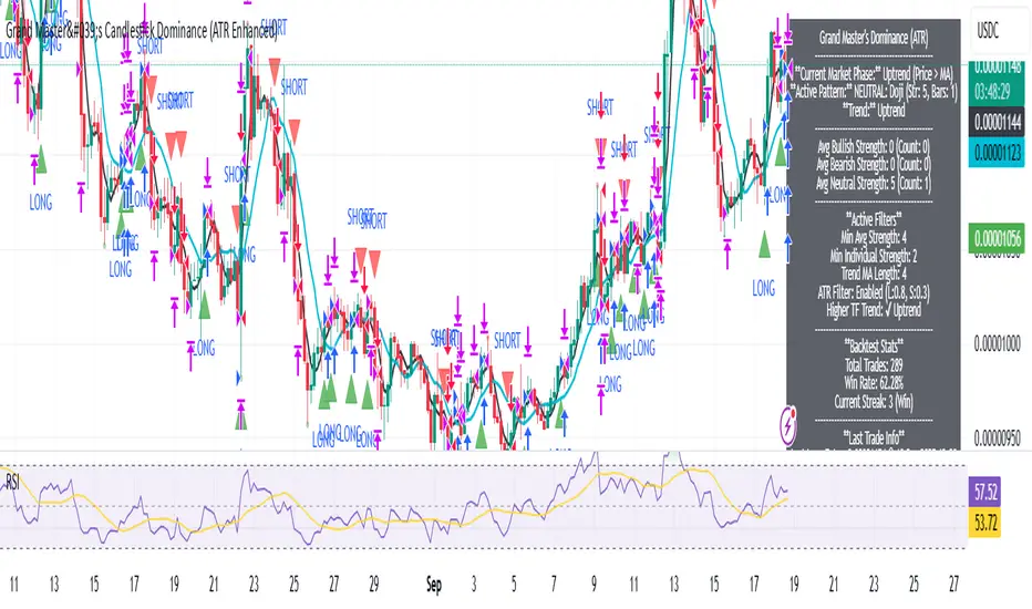
BPS Multi-MA 5 — 22/30, SMA/WMA/EMA# Multi-MA 5 — 22/30 base, SMA/WMA/EMA
**What it is**
A lightweight 5-line moving-average ribbon for fast visual bias and trend/mean-reversion reads. You can switch the MA type (SMA/WMA/EMA) and choose between two ways of setting lengths: by monthly “session-based” base (22 or 30) with multipliers, or by entering exact lengths manually. An optional info table shows the effective settings in real time.
---
## How it works
* Calculates five moving averages from the selected price source.
* Lengths are either:
* **Multipliers mode:** `Base × Multiplier` (e.g., base 22 → 22/44/66/88/110), or
* **Manual mode:** any five exact lengths (e.g., 10/22/50/100/200).
* Plots five lines with fixed legend titles (MA1…MA5); the **info table** displays the actual type and lengths.
---
## Inputs
**Length Mode**
* **Multipliers** — choose a **Base** of **22** (≈ trading sessions per month) or **30** (calendar-style, smoother) and set **×1…×5** multipliers.
* **Manual** — enter **Len1…Len5** directly.
**MA Settings**
* **MA Type:** SMA / WMA / EMA
* **Source:** any series (e.g., `close`, `hlc3`, etc.)
* **Use true close (ignore Heikin Ashi):** when enabled, the MA is computed from the underlying instrument’s real `close`, not HA candles.
* **Show info table:** toggles the on-chart table with the current mode, type, base, and lengths.
---
## Quick start
1. Add the indicator to your chart.
2. Pick **MA Type** (e.g., **WMA** for faster response, **SMA** for smoother).
3. Choose **Length Mode**:
* **Multipliers:** set **Base = 22** for session-based monthly lengths (stocks/FX), or **30** for heavier smoothing.
* **Manual:** enter your exact lengths (e.g., 10/22/50/100/200).
4. (Optional) On **Heikin Ashi** charts, enable **Use true close** if you want the lines based on the instrument’s real close.
---
## Tips & notes
* **1 month ≈ 21–22 sessions.** Using 30 as “monthly” yields a smoother, more delayed curve.
* **WMA** reacts faster than **SMA** at the same length; expect earlier signals but more whipsaws in chop.
* **Len = 1** makes the MA track the chosen source (e.g., `close`) almost exactly.
* If changing lengths doesn’t move the lines, ensure you’re editing fields for the **active Length Mode** (Multipliers vs Manual).
* For clean comparisons, use the **same timeframe**. If you later wrap this in MTF logic, keep `lookahead_off` and handle gaps appropriately.
---
## Use cases
* Trend ribbon and dynamic bias zones
* Pullback entries to the mid/slow lines
* Crossovers (fast vs slow) for confirmation
* Volatility filtering by spreading lengths (e.g., 22/44/88/132/176)
---
**Credits:** Built for clarity and speed; designed around session-based “monthly” lengths (22) or smoother calendar-style (30).

Markov Chain [3D] | FractalystWhat exactly is a Markov Chain?
This indicator uses a Markov Chain model to analyze, quantify, and visualize the transitions between market regimes (Bull, Bear, Neutral) on your chart. It dynamically detects these regimes in real-time, calculates transition probabilities, and displays them as animated 3D spheres and arrows, giving traders intuitive insight into current and future market conditions.
How does a Markov Chain work, and how should I read this spheres-and-arrows diagram?
Think of three weather modes: Sunny, Rainy, Cloudy.
Each sphere is one mode. The loop on a sphere means “stay the same next step” (e.g., Sunny again tomorrow).
The arrows leaving a sphere show where things usually go next if they change (e.g., Sunny moving to Cloudy).
Some paths matter more than others. A more prominent loop means the current mode tends to persist. A more prominent outgoing arrow means a change to that destination is the usual next step.
Direction isn’t symmetric: moving Sunny→Cloudy can behave differently than Cloudy→Sunny.
Now relabel the spheres to markets: Bull, Bear, Neutral.
Spheres: market regimes (uptrend, downtrend, range).
Self‑loop: tendency for the current regime to continue on the next bar.
Arrows: the most common next regime if a switch happens.
How to read: Start at the sphere that matches current bar state. If the loop stands out, expect continuation. If one outgoing path stands out, that switch is the typical next step. Opposite directions can differ (Bear→Neutral doesn’t have to match Neutral→Bear).
What states and transitions are shown?
The three market states visualized are:
Bullish (Bull): Upward or strong-market regime.
Bearish (Bear): Downward or weak-market regime.
Neutral: Sideways or range-bound regime.
Bidirectional animated arrows and probability labels show how likely the market is to move from one regime to another (e.g., Bull → Bear or Neutral → Bull).
How does the regime detection system work?
You can use either built-in price returns (based on adaptive Z-score normalization) or supply three custom indicators (such as volume, oscillators, etc.).
Values are statistically normalized (Z-scored) over a configurable lookback period.
The normalized outputs are classified into Bull, Bear, or Neutral zones.
If using three indicators, their regime signals are averaged and smoothed for robustness.
How are transition probabilities calculated?
On every confirmed bar, the algorithm tracks the sequence of detected market states, then builds a rolling window of transitions.
The code maintains a transition count matrix for all regime pairs (e.g., Bull → Bear).
Transition probabilities are extracted for each possible state change using Laplace smoothing for numerical stability, and frequently updated in real-time.
What is unique about the visualization?
3D animated spheres represent each regime and change visually when active.
Animated, bidirectional arrows reveal transition probabilities and allow you to see both dominant and less likely regime flows.
Particles (moving dots) animate along the arrows, enhancing the perception of regime flow direction and speed.
All elements dynamically update with each new price bar, providing a live market map in an intuitive, engaging format.
Can I use custom indicators for regime classification?
Yes! Enable the "Custom Indicators" switch and select any three chart series as inputs. These will be normalized and combined (each with equal weight), broadening the regime classification beyond just price-based movement.
What does the “Lookback Period” control?
Lookback Period (default: 100) sets how much historical data builds the probability matrix. Shorter periods adapt faster to regime changes but may be noisier. Longer periods are more stable but slower to adapt.
How is this different from a Hidden Markov Model (HMM)?
It sets the window for both regime detection and probability calculations. Lower values make the system more reactive, but potentially noisier. Higher values smooth estimates and make the system more robust.
How is this Markov Chain different from a Hidden Markov Model (HMM)?
Markov Chain (as here): All market regimes (Bull, Bear, Neutral) are directly observable on the chart. The transition matrix is built from actual detected regimes, keeping the model simple and interpretable.
Hidden Markov Model: The actual regimes are unobservable ("hidden") and must be inferred from market output or indicator "emissions" using statistical learning algorithms. HMMs are more complex, can capture more subtle structure, but are harder to visualize and require additional machine learning steps for training.
A standard Markov Chain models transitions between observable states using a simple transition matrix, while a Hidden Markov Model assumes the true states are hidden (latent) and must be inferred from observable “emissions” like price or volume data. In practical terms, a Markov Chain is transparent and easier to implement and interpret; an HMM is more expressive but requires statistical inference to estimate hidden states from data.
Markov Chain: states are observable; you directly count or estimate transition probabilities between visible states. This makes it simpler, faster, and easier to validate and tune.
HMM: states are hidden; you only observe emissions generated by those latent states. Learning involves machine learning/statistical algorithms (commonly Baum–Welch/EM for training and Viterbi for decoding) to infer both the transition dynamics and the most likely hidden state sequence from data.
How does the indicator avoid “repainting” or look-ahead bias?
All regime changes and matrix updates happen only on confirmed (closed) bars, so no future data is leaked, ensuring reliable real-time operation.
Are there practical tuning tips?
Tune the Lookback Period for your asset/timeframe: shorter for fast markets, longer for stability.
Use custom indicators if your asset has unique regime drivers.
Watch for rapid changes in transition probabilities as early warning of a possible regime shift.
Who is this indicator for?
Quants and quantitative researchers exploring probabilistic market modeling, especially those interested in regime-switching dynamics and Markov models.
Programmers and system developers who need a probabilistic regime filter for systematic and algorithmic backtesting:
The Markov Chain indicator is ideally suited for programmatic integration via its bias output (1 = Bull, 0 = Neutral, -1 = Bear).
Although the visualization is engaging, the core output is designed for automated, rules-based workflows—not for discretionary/manual trading decisions.
Developers can connect the indicator’s output directly to their Pine Script logic (using input.source()), allowing rapid and robust backtesting of regime-based strategies.
It acts as a plug-and-play regime filter: simply plug the bias output into your entry/exit logic, and you have a scientifically robust, probabilistically-derived signal for filtering, timing, position sizing, or risk regimes.
The MC's output is intentionally "trinary" (1/0/-1), focusing on clear regime states for unambiguous decision-making in code. If you require nuanced, multi-probability or soft-label state vectors, consider expanding the indicator or stacking it with a probability-weighted logic layer in your scripting.
Because it avoids subjectivity, this approach is optimal for systematic quants, algo developers building backtested, repeatable strategies based on probabilistic regime analysis.
What's the mathematical foundation behind this?
The mathematical foundation behind this Markov Chain indicator—and probabilistic regime detection in finance—draws from two principal models: the (standard) Markov Chain and the Hidden Markov Model (HMM).
How to use this indicator programmatically?
The Markov Chain indicator automatically exports a bias value (+1 for Bullish, -1 for Bearish, 0 for Neutral) as a plot visible in the Data Window. This allows you to integrate its regime signal into your own scripts and strategies for backtesting, automation, or live trading.
Step-by-Step Integration with Pine Script (input.source)
Add the Markov Chain indicator to your chart.
This must be done first, since your custom script will "pull" the bias signal from the indicator's plot.
In your strategy, create an input using input.source()
Example:
//@version=5
strategy("MC Bias Strategy Example")
mcBias = input.source(close, "MC Bias Source")
After saving, go to your script’s settings. For the “MC Bias Source” input, select the plot/output of the Markov Chain indicator (typically its bias plot).
Use the bias in your trading logic
Example (long only on Bull, flat otherwise):
if mcBias == 1
strategy.entry("Long", strategy.long)
else
strategy.close("Long")
For more advanced workflows, combine mcBias with additional filters or trailing stops.
How does this work behind-the-scenes?
TradingView’s input.source() lets you use any plot from another indicator as a real-time, “live” data feed in your own script (source).
The selected bias signal is available to your Pine code as a variable, enabling logical decisions based on regime (trend-following, mean-reversion, etc.).
This enables powerful strategy modularity : decouple regime detection from entry/exit logic, allowing fast experimentation without rewriting core signal code.
Integrating 45+ Indicators with Your Markov Chain — How & Why
The Enhanced Custom Indicators Export script exports a massive suite of over 45 technical indicators—ranging from classic momentum (RSI, MACD, Stochastic, etc.) to trend, volume, volatility, and oscillator tools—all pre-calculated, centered/scaled, and available as plots.
// Enhanced Custom Indicators Export - 45 Technical Indicators
// Comprehensive technical analysis suite for advanced market regime detection
//@version=6
indicator('Enhanced Custom Indicators Export | Fractalyst', shorttitle='Enhanced CI Export', overlay=false, scale=scale.right, max_labels_count=500, max_lines_count=500)
// |----- Input Parameters -----| //
momentum_group = "Momentum Indicators"
trend_group = "Trend Indicators"
volume_group = "Volume Indicators"
volatility_group = "Volatility Indicators"
oscillator_group = "Oscillator Indicators"
display_group = "Display Settings"
// Common lengths
length_14 = input.int(14, "Standard Length (14)", minval=1, maxval=100, group=momentum_group)
length_20 = input.int(20, "Medium Length (20)", minval=1, maxval=200, group=trend_group)
length_50 = input.int(50, "Long Length (50)", minval=1, maxval=200, group=trend_group)
// Display options
show_table = input.bool(true, "Show Values Table", group=display_group)
table_size = input.string("Small", "Table Size", options= , group=display_group)
// |----- MOMENTUM INDICATORS (15 indicators) -----| //
// 1. RSI (Relative Strength Index)
rsi_14 = ta.rsi(close, length_14)
rsi_centered = rsi_14 - 50
// 2. Stochastic Oscillator
stoch_k = ta.stoch(close, high, low, length_14)
stoch_d = ta.sma(stoch_k, 3)
stoch_centered = stoch_k - 50
// 3. Williams %R
williams_r = ta.stoch(close, high, low, length_14) - 100
// 4. MACD (Moving Average Convergence Divergence)
= ta.macd(close, 12, 26, 9)
// 5. Momentum (Rate of Change)
momentum = ta.mom(close, length_14)
momentum_pct = (momentum / close ) * 100
// 6. Rate of Change (ROC)
roc = ta.roc(close, length_14)
// 7. Commodity Channel Index (CCI)
cci = ta.cci(close, length_20)
// 8. Money Flow Index (MFI)
mfi = ta.mfi(close, length_14)
mfi_centered = mfi - 50
// 9. Awesome Oscillator (AO)
ao = ta.sma(hl2, 5) - ta.sma(hl2, 34)
// 10. Accelerator Oscillator (AC)
ac = ao - ta.sma(ao, 5)
// 11. Chande Momentum Oscillator (CMO)
cmo = ta.cmo(close, length_14)
// 12. Detrended Price Oscillator (DPO)
dpo = close - ta.sma(close, length_20)
// 13. Price Oscillator (PPO)
ppo = ta.sma(close, 12) - ta.sma(close, 26)
ppo_pct = (ppo / ta.sma(close, 26)) * 100
// 14. TRIX
trix_ema1 = ta.ema(close, length_14)
trix_ema2 = ta.ema(trix_ema1, length_14)
trix_ema3 = ta.ema(trix_ema2, length_14)
trix = ta.roc(trix_ema3, 1) * 10000
// 15. Klinger Oscillator
klinger = ta.ema(volume * (high + low + close) / 3, 34) - ta.ema(volume * (high + low + close) / 3, 55)
// 16. Fisher Transform
fisher_hl2 = 0.5 * (hl2 - ta.lowest(hl2, 10)) / (ta.highest(hl2, 10) - ta.lowest(hl2, 10)) - 0.25
fisher = 0.5 * math.log((1 + fisher_hl2) / (1 - fisher_hl2))
// 17. Stochastic RSI
stoch_rsi = ta.stoch(rsi_14, rsi_14, rsi_14, length_14)
stoch_rsi_centered = stoch_rsi - 50
// 18. Relative Vigor Index (RVI)
rvi_num = ta.swma(close - open)
rvi_den = ta.swma(high - low)
rvi = rvi_den != 0 ? rvi_num / rvi_den : 0
// 19. Balance of Power (BOP)
bop = (close - open) / (high - low)
// |----- TREND INDICATORS (10 indicators) -----| //
// 20. Simple Moving Average Momentum
sma_20 = ta.sma(close, length_20)
sma_momentum = ((close - sma_20) / sma_20) * 100
// 21. Exponential Moving Average Momentum
ema_20 = ta.ema(close, length_20)
ema_momentum = ((close - ema_20) / ema_20) * 100
// 22. Parabolic SAR
sar = ta.sar(0.02, 0.02, 0.2)
sar_trend = close > sar ? 1 : -1
// 23. Linear Regression Slope
lr_slope = ta.linreg(close, length_20, 0) - ta.linreg(close, length_20, 1)
// 24. Moving Average Convergence (MAC)
mac = ta.sma(close, 10) - ta.sma(close, 30)
// 25. Trend Intensity Index (TII)
tii_sum = 0.0
for i = 1 to length_20
tii_sum += close > close ? 1 : 0
tii = (tii_sum / length_20) * 100
// 26. Ichimoku Cloud Components
ichimoku_tenkan = (ta.highest(high, 9) + ta.lowest(low, 9)) / 2
ichimoku_kijun = (ta.highest(high, 26) + ta.lowest(low, 26)) / 2
ichimoku_signal = ichimoku_tenkan > ichimoku_kijun ? 1 : -1
// 27. MESA Adaptive Moving Average (MAMA)
mama_alpha = 2.0 / (length_20 + 1)
mama = ta.ema(close, length_20)
mama_momentum = ((close - mama) / mama) * 100
// 28. Zero Lag Exponential Moving Average (ZLEMA)
zlema_lag = math.round((length_20 - 1) / 2)
zlema_data = close + (close - close )
zlema = ta.ema(zlema_data, length_20)
zlema_momentum = ((close - zlema) / zlema) * 100
// |----- VOLUME INDICATORS (6 indicators) -----| //
// 29. On-Balance Volume (OBV)
obv = ta.obv
// 30. Volume Rate of Change (VROC)
vroc = ta.roc(volume, length_14)
// 31. Price Volume Trend (PVT)
pvt = ta.pvt
// 32. Negative Volume Index (NVI)
nvi = 0.0
nvi := volume < volume ? nvi + ((close - close ) / close ) * nvi : nvi
// 33. Positive Volume Index (PVI)
pvi = 0.0
pvi := volume > volume ? pvi + ((close - close ) / close ) * pvi : pvi
// 34. Volume Oscillator
vol_osc = ta.sma(volume, 5) - ta.sma(volume, 10)
// 35. Ease of Movement (EOM)
eom_distance = high - low
eom_box_height = volume / 1000000
eom = eom_box_height != 0 ? eom_distance / eom_box_height : 0
eom_sma = ta.sma(eom, length_14)
// 36. Force Index
force_index = volume * (close - close )
force_index_sma = ta.sma(force_index, length_14)
// |----- VOLATILITY INDICATORS (10 indicators) -----| //
// 37. Average True Range (ATR)
atr = ta.atr(length_14)
atr_pct = (atr / close) * 100
// 38. Bollinger Bands Position
bb_basis = ta.sma(close, length_20)
bb_dev = 2.0 * ta.stdev(close, length_20)
bb_upper = bb_basis + bb_dev
bb_lower = bb_basis - bb_dev
bb_position = bb_dev != 0 ? (close - bb_basis) / bb_dev : 0
bb_width = bb_dev != 0 ? (bb_upper - bb_lower) / bb_basis * 100 : 0
// 39. Keltner Channels Position
kc_basis = ta.ema(close, length_20)
kc_range = ta.ema(ta.tr, length_20)
kc_upper = kc_basis + (2.0 * kc_range)
kc_lower = kc_basis - (2.0 * kc_range)
kc_position = kc_range != 0 ? (close - kc_basis) / kc_range : 0
// 40. Donchian Channels Position
dc_upper = ta.highest(high, length_20)
dc_lower = ta.lowest(low, length_20)
dc_basis = (dc_upper + dc_lower) / 2
dc_position = (dc_upper - dc_lower) != 0 ? (close - dc_basis) / (dc_upper - dc_lower) : 0
// 41. Standard Deviation
std_dev = ta.stdev(close, length_20)
std_dev_pct = (std_dev / close) * 100
// 42. Relative Volatility Index (RVI)
rvi_up = ta.stdev(close > close ? close : 0, length_14)
rvi_down = ta.stdev(close < close ? close : 0, length_14)
rvi_total = rvi_up + rvi_down
rvi_volatility = rvi_total != 0 ? (rvi_up / rvi_total) * 100 : 50
// 43. Historical Volatility
hv_returns = math.log(close / close )
hv = ta.stdev(hv_returns, length_20) * math.sqrt(252) * 100
// 44. Garman-Klass Volatility
gk_vol = math.log(high/low) * math.log(high/low) - (2*math.log(2)-1) * math.log(close/open) * math.log(close/open)
gk_volatility = math.sqrt(ta.sma(gk_vol, length_20)) * 100
// 45. Parkinson Volatility
park_vol = math.log(high/low) * math.log(high/low)
parkinson = math.sqrt(ta.sma(park_vol, length_20) / (4 * math.log(2))) * 100
// 46. Rogers-Satchell Volatility
rs_vol = math.log(high/close) * math.log(high/open) + math.log(low/close) * math.log(low/open)
rogers_satchell = math.sqrt(ta.sma(rs_vol, length_20)) * 100
// |----- OSCILLATOR INDICATORS (5 indicators) -----| //
// 47. Elder Ray Index
elder_bull = high - ta.ema(close, 13)
elder_bear = low - ta.ema(close, 13)
elder_power = elder_bull + elder_bear
// 48. Schaff Trend Cycle (STC)
stc_macd = ta.ema(close, 23) - ta.ema(close, 50)
stc_k = ta.stoch(stc_macd, stc_macd, stc_macd, 10)
stc_d = ta.ema(stc_k, 3)
stc = ta.stoch(stc_d, stc_d, stc_d, 10)
// 49. Coppock Curve
coppock_roc1 = ta.roc(close, 14)
coppock_roc2 = ta.roc(close, 11)
coppock = ta.wma(coppock_roc1 + coppock_roc2, 10)
// 50. Know Sure Thing (KST)
kst_roc1 = ta.roc(close, 10)
kst_roc2 = ta.roc(close, 15)
kst_roc3 = ta.roc(close, 20)
kst_roc4 = ta.roc(close, 30)
kst = ta.sma(kst_roc1, 10) + 2*ta.sma(kst_roc2, 10) + 3*ta.sma(kst_roc3, 10) + 4*ta.sma(kst_roc4, 15)
// 51. Percentage Price Oscillator (PPO)
ppo_line = ((ta.ema(close, 12) - ta.ema(close, 26)) / ta.ema(close, 26)) * 100
ppo_signal = ta.ema(ppo_line, 9)
ppo_histogram = ppo_line - ppo_signal
// |----- PLOT MAIN INDICATORS -----| //
// Plot key momentum indicators
plot(rsi_centered, title="01_RSI_Centered", color=color.purple, linewidth=1)
plot(stoch_centered, title="02_Stoch_Centered", color=color.blue, linewidth=1)
plot(williams_r, title="03_Williams_R", color=color.red, linewidth=1)
plot(macd_histogram, title="04_MACD_Histogram", color=color.orange, linewidth=1)
plot(cci, title="05_CCI", color=color.green, linewidth=1)
// Plot trend indicators
plot(sma_momentum, title="06_SMA_Momentum", color=color.navy, linewidth=1)
plot(ema_momentum, title="07_EMA_Momentum", color=color.maroon, linewidth=1)
plot(sar_trend, title="08_SAR_Trend", color=color.teal, linewidth=1)
plot(lr_slope, title="09_LR_Slope", color=color.lime, linewidth=1)
plot(mac, title="10_MAC", color=color.fuchsia, linewidth=1)
// Plot volatility indicators
plot(atr_pct, title="11_ATR_Pct", color=color.yellow, linewidth=1)
plot(bb_position, title="12_BB_Position", color=color.aqua, linewidth=1)
plot(kc_position, title="13_KC_Position", color=color.olive, linewidth=1)
plot(std_dev_pct, title="14_StdDev_Pct", color=color.silver, linewidth=1)
plot(bb_width, title="15_BB_Width", color=color.gray, linewidth=1)
// Plot volume indicators
plot(vroc, title="16_VROC", color=color.blue, linewidth=1)
plot(eom_sma, title="17_EOM", color=color.red, linewidth=1)
plot(vol_osc, title="18_Vol_Osc", color=color.green, linewidth=1)
plot(force_index_sma, title="19_Force_Index", color=color.orange, linewidth=1)
plot(obv, title="20_OBV", color=color.purple, linewidth=1)
// Plot additional oscillators
plot(ao, title="21_Awesome_Osc", color=color.navy, linewidth=1)
plot(cmo, title="22_CMO", color=color.maroon, linewidth=1)
plot(dpo, title="23_DPO", color=color.teal, linewidth=1)
plot(trix, title="24_TRIX", color=color.lime, linewidth=1)
plot(fisher, title="25_Fisher", color=color.fuchsia, linewidth=1)
// Plot more momentum indicators
plot(mfi_centered, title="26_MFI_Centered", color=color.yellow, linewidth=1)
plot(ac, title="27_AC", color=color.aqua, linewidth=1)
plot(ppo_pct, title="28_PPO_Pct", color=color.olive, linewidth=1)
plot(stoch_rsi_centered, title="29_StochRSI_Centered", color=color.silver, linewidth=1)
plot(klinger, title="30_Klinger", color=color.gray, linewidth=1)
// Plot trend continuation
plot(tii, title="31_TII", color=color.blue, linewidth=1)
plot(ichimoku_signal, title="32_Ichimoku_Signal", color=color.red, linewidth=1)
plot(mama_momentum, title="33_MAMA_Momentum", color=color.green, linewidth=1)
plot(zlema_momentum, title="34_ZLEMA_Momentum", color=color.orange, linewidth=1)
plot(bop, title="35_BOP", color=color.purple, linewidth=1)
// Plot volume continuation
plot(nvi, title="36_NVI", color=color.navy, linewidth=1)
plot(pvi, title="37_PVI", color=color.maroon, linewidth=1)
plot(momentum_pct, title="38_Momentum_Pct", color=color.teal, linewidth=1)
plot(roc, title="39_ROC", color=color.lime, linewidth=1)
plot(rvi, title="40_RVI", color=color.fuchsia, linewidth=1)
// Plot volatility continuation
plot(dc_position, title="41_DC_Position", color=color.yellow, linewidth=1)
plot(rvi_volatility, title="42_RVI_Volatility", color=color.aqua, linewidth=1)
plot(hv, title="43_Historical_Vol", color=color.olive, linewidth=1)
plot(gk_volatility, title="44_GK_Volatility", color=color.silver, linewidth=1)
plot(parkinson, title="45_Parkinson_Vol", color=color.gray, linewidth=1)
// Plot final oscillators
plot(rogers_satchell, title="46_RS_Volatility", color=color.blue, linewidth=1)
plot(elder_power, title="47_Elder_Power", color=color.red, linewidth=1)
plot(stc, title="48_STC", color=color.green, linewidth=1)
plot(coppock, title="49_Coppock", color=color.orange, linewidth=1)
plot(kst, title="50_KST", color=color.purple, linewidth=1)
// Plot final indicators
plot(ppo_histogram, title="51_PPO_Histogram", color=color.navy, linewidth=1)
plot(pvt, title="52_PVT", color=color.maroon, linewidth=1)
// |----- Reference Lines -----| //
hline(0, "Zero Line", color=color.gray, linestyle=hline.style_dashed, linewidth=1)
hline(50, "Midline", color=color.gray, linestyle=hline.style_dotted, linewidth=1)
hline(-50, "Lower Midline", color=color.gray, linestyle=hline.style_dotted, linewidth=1)
hline(25, "Upper Threshold", color=color.gray, linestyle=hline.style_dotted, linewidth=1)
hline(-25, "Lower Threshold", color=color.gray, linestyle=hline.style_dotted, linewidth=1)
// |----- Enhanced Information Table -----| //
if show_table and barstate.islast
table_position = position.top_right
table_text_size = table_size == "Tiny" ? size.tiny : table_size == "Small" ? size.small : size.normal
var table info_table = table.new(table_position, 3, 18, bgcolor=color.new(color.white, 85), border_width=1, border_color=color.gray)
// Headers
table.cell(info_table, 0, 0, 'Category', text_color=color.black, text_size=table_text_size, bgcolor=color.new(color.blue, 70))
table.cell(info_table, 1, 0, 'Indicator', text_color=color.black, text_size=table_text_size, bgcolor=color.new(color.blue, 70))
table.cell(info_table, 2, 0, 'Value', text_color=color.black, text_size=table_text_size, bgcolor=color.new(color.blue, 70))
// Key Momentum Indicators
table.cell(info_table, 0, 1, 'MOMENTUM', text_color=color.purple, text_size=table_text_size, bgcolor=color.new(color.purple, 90))
table.cell(info_table, 1, 1, 'RSI Centered', text_color=color.purple, text_size=table_text_size)
table.cell(info_table, 2, 1, str.tostring(rsi_centered, '0.00'), text_color=color.purple, text_size=table_text_size)
table.cell(info_table, 0, 2, '', text_color=color.blue, text_size=table_text_size)
table.cell(info_table, 1, 2, 'Stoch Centered', text_color=color.blue, text_size=table_text_size)
table.cell(info_table, 2, 2, str.tostring(stoch_centered, '0.00'), text_color=color.blue, text_size=table_text_size)
table.cell(info_table, 0, 3, '', text_color=color.red, text_size=table_text_size)
table.cell(info_table, 1, 3, 'Williams %R', text_color=color.red, text_size=table_text_size)
table.cell(info_table, 2, 3, str.tostring(williams_r, '0.00'), text_color=color.red, text_size=table_text_size)
table.cell(info_table, 0, 4, '', text_color=color.orange, text_size=table_text_size)
table.cell(info_table, 1, 4, 'MACD Histogram', text_color=color.orange, text_size=table_text_size)
table.cell(info_table, 2, 4, str.tostring(macd_histogram, '0.000'), text_color=color.orange, text_size=table_text_size)
table.cell(info_table, 0, 5, '', text_color=color.green, text_size=table_text_size)
table.cell(info_table, 1, 5, 'CCI', text_color=color.green, text_size=table_text_size)
table.cell(info_table, 2, 5, str.tostring(cci, '0.00'), text_color=color.green, text_size=table_text_size)
// Key Trend Indicators
table.cell(info_table, 0, 6, 'TREND', text_color=color.navy, text_size=table_text_size, bgcolor=color.new(color.navy, 90))
table.cell(info_table, 1, 6, 'SMA Momentum %', text_color=color.navy, text_size=table_text_size)
table.cell(info_table, 2, 6, str.tostring(sma_momentum, '0.00'), text_color=color.navy, text_size=table_text_size)
table.cell(info_table, 0, 7, '', text_color=color.maroon, text_size=table_text_size)
table.cell(info_table, 1, 7, 'EMA Momentum %', text_color=color.maroon, text_size=table_text_size)
table.cell(info_table, 2, 7, str.tostring(ema_momentum, '0.00'), text_color=color.maroon, text_size=table_text_size)
table.cell(info_table, 0, 8, '', text_color=color.teal, text_size=table_text_size)
table.cell(info_table, 1, 8, 'SAR Trend', text_color=color.teal, text_size=table_text_size)
table.cell(info_table, 2, 8, str.tostring(sar_trend, '0'), text_color=color.teal, text_size=table_text_size)
table.cell(info_table, 0, 9, '', text_color=color.lime, text_size=table_text_size)
table.cell(info_table, 1, 9, 'Linear Regression', text_color=color.lime, text_size=table_text_size)
table.cell(info_table, 2, 9, str.tostring(lr_slope, '0.000'), text_color=color.lime, text_size=table_text_size)
// Key Volatility Indicators
table.cell(info_table, 0, 10, 'VOLATILITY', text_color=color.yellow, text_size=table_text_size, bgcolor=color.new(color.yellow, 90))
table.cell(info_table, 1, 10, 'ATR %', text_color=color.yellow, text_size=table_text_size)
table.cell(info_table, 2, 10, str.tostring(atr_pct, '0.00'), text_color=color.yellow, text_size=table_text_size)
table.cell(info_table, 0, 11, '', text_color=color.aqua, text_size=table_text_size)
table.cell(info_table, 1, 11, 'BB Position', text_color=color.aqua, text_size=table_text_size)
table.cell(info_table, 2, 11, str.tostring(bb_position, '0.00'), text_color=color.aqua, text_size=table_text_size)
table.cell(info_table, 0, 12, '', text_color=color.olive, text_size=table_text_size)
table.cell(info_table, 1, 12, 'KC Position', text_color=color.olive, text_size=table_text_size)
table.cell(info_table, 2, 12, str.tostring(kc_position, '0.00'), text_color=color.olive, text_size=table_text_size)
// Key Volume Indicators
table.cell(info_table, 0, 13, 'VOLUME', text_color=color.blue, text_size=table_text_size, bgcolor=color.new(color.blue, 90))
table.cell(info_table, 1, 13, 'Volume ROC', text_color=color.blue, text_size=table_text_size)
table.cell(info_table, 2, 13, str.tostring(vroc, '0.00'), text_color=color.blue, text_size=table_text_size)
table.cell(info_table, 0, 14, '', text_color=color.red, text_size=table_text_size)
table.cell(info_table, 1, 14, 'EOM', text_color=color.red, text_size=table_text_size)
table.cell(info_table, 2, 14, str.tostring(eom_sma, '0.000'), text_color=color.red, text_size=table_text_size)
// Key Oscillators
table.cell(info_table, 0, 15, 'OSCILLATORS', text_color=color.purple, text_size=table_text_size, bgcolor=color.new(color.purple, 90))
table.cell(info_table, 1, 15, 'Awesome Osc', text_color=color.blue, text_size=table_text_size)
table.cell(info_table, 2, 15, str.tostring(ao, '0.000'), text_color=color.blue, text_size=table_text_size)
table.cell(info_table, 0, 16, '', text_color=color.red, text_size=table_text_size)
table.cell(info_table, 1, 16, 'Fisher Transform', text_color=color.red, text_size=table_text_size)
table.cell(info_table, 2, 16, str.tostring(fisher, '0.000'), text_color=color.red, text_size=table_text_size)
// Summary Statistics
table.cell(info_table, 0, 17, 'SUMMARY', text_color=color.black, text_size=table_text_size, bgcolor=color.new(color.gray, 70))
table.cell(info_table, 1, 17, 'Total Indicators: 52', text_color=color.black, text_size=table_text_size)
regime_color = rsi_centered > 10 ? color.green : rsi_centered < -10 ? color.red : color.gray
regime_text = rsi_centered > 10 ? "BULLISH" : rsi_centered < -10 ? "BEARISH" : "NEUTRAL"
table.cell(info_table, 2, 17, regime_text, text_color=regime_color, text_size=table_text_size)
This makes it the perfect “indicator backbone” for quantitative and systematic traders who want to prototype, combine, and test new regime detection models—especially in combination with the Markov Chain indicator.
How to use this script with the Markov Chain for research and backtesting:
Add the Enhanced Indicator Export to your chart.
Every calculated indicator is available as an individual data stream.
Connect the indicator(s) you want as custom input(s) to the Markov Chain’s “Custom Indicators” option.
In the Markov Chain indicator’s settings, turn ON the custom indicator mode.
For each of the three custom indicator inputs, select the exported plot from the Enhanced Export script—the menu lists all 45+ signals by name.
This creates a powerful, modular regime-detection engine where you can mix-and-match momentum, trend, volume, or custom combinations for advanced filtering.
Backtest regime logic directly.
Once you’ve connected your chosen indicators, the Markov Chain script performs regime detection (Bull/Neutral/Bear) based on your selected features—not just price returns.
The regime detection is robust, automatically normalized (using Z-score), and outputs bias (1, -1, 0) for plug-and-play integration.
Export the regime bias for programmatic use.
As described above, use input.source() in your Pine Script strategy or system and link the bias output.
You can now filter signals, control trade direction/size, or design pairs-trading that respect true, indicator-driven market regimes.
With this framework, you’re not limited to static or simplistic regime filters. You can rigorously define, test, and refine what “market regime” means for your strategies—using the technical features that matter most to you.
Optimize your signal generation by backtesting across a universe of meaningful indicator blends.
Enhance risk management with objective, real-time regime boundaries.
Accelerate your research: iterate quickly, swap indicator components, and see results with minimal code changes.
Automate multi-asset or pairs-trading by integrating regime context directly into strategy logic.
Add both scripts to your chart, connect your preferred features, and start investigating your best regime-based trades—entirely within the TradingView ecosystem.
References & Further Reading
Ang, A., & Bekaert, G. (2002). “Regime Switches in Interest Rates.” Journal of Business & Economic Statistics, 20(2), 163–182.
Hamilton, J. D. (1989). “A New Approach to the Economic Analysis of Nonstationary Time Series and the Business Cycle.” Econometrica, 57(2), 357–384.
Markov, A. A. (1906). "Extension of the Limit Theorems of Probability Theory to a Sum of Variables Connected in a Chain." The Notes of the Imperial Academy of Sciences of St. Petersburg.
Guidolin, M., & Timmermann, A. (2007). “Asset Allocation under Multivariate Regime Switching.” Journal of Economic Dynamics and Control, 31(11), 3503–3544.
Murphy, J. J. (1999). Technical Analysis of the Financial Markets. New York Institute of Finance.
Brock, W., Lakonishok, J., & LeBaron, B. (1992). “Simple Technical Trading Rules and the Stochastic Properties of Stock Returns.” Journal of Finance, 47(5), 1731–1764.
Zucchini, W., MacDonald, I. L., & Langrock, R. (2017). Hidden Markov Models for Time Series: An Introduction Using R (2nd ed.). Chapman and Hall/CRC.
On Quantitative Finance and Markov Models:
Lo, A. W., & Hasanhodzic, J. (2009). The Heretics of Finance: Conversations with Leading Practitioners of Technical Analysis. Bloomberg Press.
Patterson, S. (2016). The Man Who Solved the Market: How Jim Simons Launched the Quant Revolution. Penguin Press.
TradingView Pine Script Documentation: www.tradingview.com
TradingView Blog: “Use an Input From Another Indicator With Your Strategy” www.tradingview.com
GeeksforGeeks: “What is the Difference Between Markov Chains and Hidden Markov Models?” www.geeksforgeeks.org
What makes this indicator original and unique?
- On‑chart, real‑time Markov. The chain is drawn directly on your chart. You see the current regime, its tendency to stay (self‑loop), and the usual next step (arrows) as bars confirm.
- Source‑agnostic by design. The engine runs on any series you select via input.source() — price, your own oscillator, a composite score, anything you compute in the script.
- Automatic normalization + regime mapping. Different inputs live on different scales. The script standardizes your chosen source and maps it into clear regimes (e.g., Bull / Bear / Neutral) without you micromanaging thresholds each time.
- Rolling, bar‑by‑bar learning. Transition tendencies are computed from a rolling window of confirmed bars. What you see is exactly what the market did in that window.
- Fast experimentation. Switch the source, adjust the window, and the Markov view updates instantly. It’s a rapid way to test ideas and feel regime persistence/switch behavior.
Integrate your own signals (using input.source())
- In settings, choose the Source . This is powered by input.source() .
- Feed it price, an indicator you compute inside the script, or a custom composite series.
- The script will automatically normalize that series and process it through the Markov engine, mapping it to regimes and updating the on‑chart spheres/arrows in real time.
Credits:
Deep gratitude to @RicardoSantos for both the foundational Markov chain processing engine and inspiring open-source contributions, which made advanced probabilistic market modeling accessible to the TradingView community.
Special thanks to @Alien_Algorithms for the innovative and visually stunning 3D sphere logic that powers the indicator’s animated, regime-based visualization.
Disclaimer
This tool summarizes recent behavior. It is not financial advice and not a guarantee of future results.

LANZ Strategy 6.0🔷 LANZ Strategy 6.0 — NY Session Entry Tool & Multi-Account Risk Manager
LANZ Strategy 6.0 - Is a trading tool designed to help traders plan, execute, and manage operations with a focus on risk management, multi-account handling, and visual clarity.
It works exclusively on the 1-hour timeframe ⏳ and is optimized for the New York market opening dynamics.
🧠 Core Concept
The strategy identifies bullish trading opportunities based on the 09:00 NY candle. Once detected, it automatically calculates and draws:
EP (Entry Price) — The exact level where the trade setup triggers.
SL (Stop Loss) — Based on a customizable percentage of the candle's high–low range or wick extremes.
TP (Take Profit) — Calculated using your chosen Risk–Reward Ratio (e.g., 1:5, 1:3, etc.).
⚙️ Main Features
⏳ Time-Specific Execution
Operates only when the 09:00 NY candle closes bullish.
Ideal for traders who align with the New York Session market structure.
💰 Multi-Account Lot Size Management
Up to 5 independent accounts can be configured with their own capital and risk %, showing the exact lot size to use for each.
📏 Adaptive Risk Control
Supports both Forex and non-Forex assets (indices, gold, oil).
For non-Forex, you can manually define the pip value according to your broker’s specs.
🎨 Visual Trade Map
Automatically plots clean and easy-to-read EP, SL, and TP lines with customizable colors, styles, and thickness.
A floating information panel displays levels, pip distances, and lot sizes.
🔔 Real-Time Alerts
Alerts for:
Entry signal detection.
Stop Loss hit.
Take Profit hit.
Manual close at the defined session end.
📊 Example
If you trade GBPUSD with Account #1 set to $10,000 and 2% risk,
and the 09:00 NY candle closes bullish with SL = 30 pips and RR = 5:1:
EP, SL, and TP levels are drawn instantly.
Risk = $200 (2% of $10,000).
Lot size is calculated automatically.
All details are shown in the on-chart panel.
🛠️ How to Use
Load the indicator on a 1-hour chart.
Configure risk settings and account data.
Wait for the 09:00 NY candle to close bullish.
Use the displayed lot size and levels to execute your trade.
Let the tool alert you for SL, TP, or manual close.
⚠️ Disclaimer:
This script is for educational purposes only. It does not guarantee profits and past performance does not represent future results. Always manage your risk responsibly.
👨💻 Credits:
💡 Developed by: LANZ
🧠 Execution Model & Logic Design: LANZ
📅 Designed for: 1H timeframe and NY-based entries

LANZ Strategy 7.0🔷 LANZ Strategy 7.0 — Multi-Session Breakout Logic with Midnight-Cross Support, Dynamic SL/TP, Multi-Account Lot Sizing & Real-Time Visual Tracking
LANZ Strategy 7.0 is a robust, visually-driven trading indicator designed to capture high-probability breakouts from a customizable market session.
It includes full support for sessions that cross midnight, dynamic calculation of Entry Price (EP), Stop Loss (SL) and Take Profit (TP) levels, and a multi-account lot sizing panel for precise risk management.
The system is built to only trigger one trade per day and manages the full trade lifecycle with automated visual cleanup and detailed alerts.
📌 This is an indicator, not a strategy — it does not place trades automatically, but provides exact entry setups, SL/TP levels, risk-based lot size guidance, and real-time alerts for execution.
🧠 Core Logic & Features
🚀 Entry Signal (BUY/SELL)
The trading day begins with a Decision Session (yellow box) where the high/low range is recorded.
Once the Operative Session starts (blue zone), the first touch of the session’s high triggers a BUY setup, and the first touch of the session’s low triggers a SELL setup.
Only one valid trade can be triggered per day — the system locks after the first signal.
⚙️ Dynamic Stop Loss & Take Profit
SL levels are derived from the Decision Session high/low using customizable Fibonacci multipliers (independent for BUY and SELL).
TP is dynamically calculated from the EP–SL distance using a user-defined Risk:Reward ratio (R:R).
All EP, SL, and TP levels are drawn as independent lines with customizable colors, label text size, and style.
⏳ Session & Midnight-Cross Support
Works with any custom Decision/Operative session hours, including sessions that start one day and end the next.
Properly tracks time zones using New York session time for consistency.
Includes Cutoff Time: after this limit, no new entries are allowed, and all visuals are auto-cleared if no trade was triggered.
💰 Multi-Account Risk-Based Lot Sizing
Supports up to 5 independent accounts.
Each account can have:
Own capital
Own risk percentage per trade
Lot size is auto-calculated based on:
SL distance (in pips or points)
Pip value (auto-detected for Forex or manually set for indices/commodities)
Results are displayed in a clean lot size info panel.
🖼️ Real-Time Visual Tracking
Dynamic updates to all levels during the Decision Session.
EP, SL, TP lines update if the session high/low changes before the Operative Session starts.
Trade result labels:
SL hit → “–1.00%” in red
TP hit → “+X.XX%” in green
Manual close at Operative End → shows actual % result in blue or purple.
🔔 Alerts for Every Key Event
Session start notification
EP entry triggered
SL or TP hit
Manual close at session end
Missed entry due to cutoff
🧭 Execution Flow
Decision Session (Yellow) — Capture high/low range.
Operative Session (Blue) — First touch of high = BUY setup; first touch of low = SELL setup.
Plot EP, SL, TP lines + calculate lot sizes for all active accounts.
Track trade until SL, TP, or Operative End.
If no entry triggered by Cutoff Time → clean all visuals and notify.
💡 Ideal For:
Traders who operate breakout logic on specific sessions (NY, London, Asian, or custom).
Those managing multiple accounts with strict risk per trade.
Anyone trading assets with sessions crossing midnight.
👨💻 Credits:
Developer: LANZ
Logic Design: LANZ
Built For: Multi-timeframe session breakouts with high precision.
Purpose: One-shot trade per day, risk consistency, and total visual clarity.
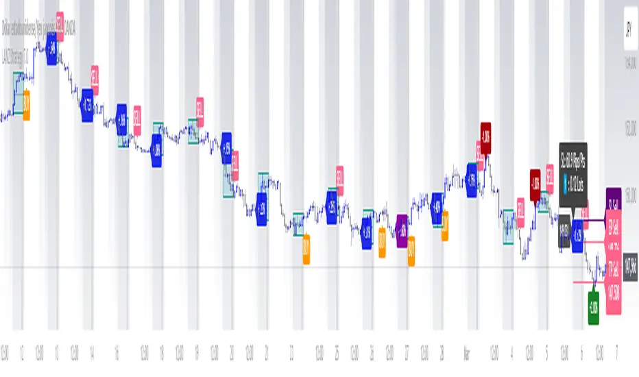
StratNinjaTableAuthor’s Instructions for StratNinjaTable
Purpose:
This indicator is designed to provide traders with a clear and dynamic table displaying The Strat candle patterns across multiple timeframes of your choice.
Usage:
Use the input panel to select which timeframes you want to monitor in the table.
Choose the table position on the chart (top left, center, right, or bottom).
The table will update each bar, showing the candle type, direction arrow, and remaining time until the candle closes for each selected timeframe.
Hover over or inspect the table to understand current market structure per timeframe using The Strat methodology.
Notes:
The Strat pattern is displayed as "1", "2U", "2D", or "3" based on the relationship of current and previous candle highs and lows.
The timer updates in real-time and adapts to daily, weekly, monthly, and extended timeframes.
This script requires Pine Script version 6. Please use it on supported platforms.
MFI or other indicators are not included in this base version but can be integrated separately if desired.
Credits:
Developed and inspired by shayy110 — thanks for your foundational work on The Strat in Pine Script.
Disclaimer:
This script is for educational and informational purposes only. Always verify signals and manage risk accordingly.
