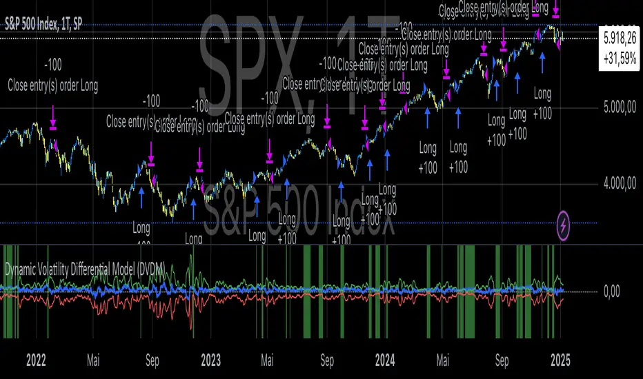
Dynamic Volatility Differential Model (DVDM)The Dynamic Volatility Differential Model (DVDM) is a quantitative trading strategy designed to exploit the spread between implied volatility (IV) and historical (realized) volatility (HV). This strategy identifies trading opportunities by dynamically adjusting thresholds based on the standard deviation of the volatility spread. The DVDM is versatile and applicable across various markets, including equity indices, commodities, and derivatives such as the FDAX (DAX Futures).
Key Components of the DVDM:
1. Implied Volatility (IV):
The IV is derived from options markets and reflects the market’s expectation of future price volatility. For instance, the strategy uses volatility indices such as the VIX (S&P 500), VXN (Nasdaq 100), or RVX (Russell 2000), depending on the target market. These indices serve as proxies for market sentiment and risk perception (Whaley, 2000).
2. Historical Volatility (HV):
The HV is computed from the log returns of the underlying asset’s price. It represents the actual volatility observed in the market over a defined lookback period, adjusted to annualized levels using a multiplier of \sqrt{252} for daily data (Hull, 2012).
3. Volatility Spread:
The difference between IV and HV forms the volatility spread, which is a measure of divergence between market expectations and actual market behavior.
4. Dynamic Thresholds:
Unlike static thresholds, the DVDM employs dynamic thresholds derived from the standard deviation of the volatility spread. The thresholds are scaled by a user-defined multiplier, ensuring adaptability to market conditions and volatility regimes (Christoffersen & Jacobs, 2004).
Trading Logic:
1. Long Entry:
A long position is initiated when the volatility spread exceeds the upper dynamic threshold, signaling that implied volatility is significantly higher than realized volatility. This condition suggests potential mean reversion, as markets may correct inflated risk premiums.
2. Short Entry:
A short position is initiated when the volatility spread falls below the lower dynamic threshold, indicating that implied volatility is significantly undervalued relative to realized volatility. This signals the possibility of increased market uncertainty.
3. Exit Conditions:
Positions are closed when the volatility spread crosses the zero line, signifying a normalization of the divergence.
Advantages of the DVDM:
1. Adaptability:
Dynamic thresholds allow the strategy to adjust to changing market conditions, making it suitable for both low-volatility and high-volatility environments.
2. Quantitative Precision:
The use of standard deviation-based thresholds enhances statistical reliability and reduces subjectivity in decision-making.
3. Market Versatility:
The strategy’s reliance on volatility metrics makes it universally applicable across asset classes and markets, ensuring robust performance.
Scientific Relevance:
The strategy builds on empirical research into the predictive power of implied volatility over realized volatility (Poon & Granger, 2003). By leveraging the divergence between these measures, the DVDM aligns with findings that IV often overestimates future volatility, creating opportunities for mean-reversion trades. Furthermore, the inclusion of dynamic thresholds aligns with risk management best practices by adapting to volatility clustering, a well-documented phenomenon in financial markets (Engle, 1982).
References:
1. Christoffersen, P., & Jacobs, K. (2004). The importance of the volatility risk premium for volatility forecasting. Journal of Financial and Quantitative Analysis, 39(2), 375-397.
2. Engle, R. F. (1982). Autoregressive conditional heteroskedasticity with estimates of the variance of United Kingdom inflation. Econometrica, 50(4), 987-1007.
3. Hull, J. C. (2012). Options, Futures, and Other Derivatives. Pearson Education.
4. Poon, S. H., & Granger, C. W. J. (2003). Forecasting volatility in financial markets: A review. Journal of Economic Literature, 41(2), 478-539.
5. Whaley, R. E. (2000). The investor fear gauge. Journal of Portfolio Management, 26(3), 12-17.
This strategy leverages quantitative techniques and statistical rigor to provide a systematic approach to volatility trading, making it a valuable tool for professional traders and quantitative analysts.
"Futures" için komut dosyalarını ara
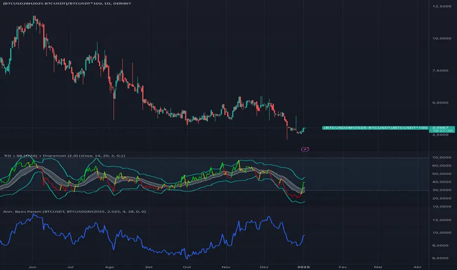
Cash and Carry: Annualized BTC Basis (Parametric)This indicator calculates the annualized BTC basis (premium or discount) between a specified futures contract and a given spot symbol. You can customize the spot ticker, the futures ticker, and the exact expiration date/time. As time moves toward expiration, the annualized yield (basis) will adjust accordingly. Ideal for monitoring potential arbitrage or cash-and-carry opportunities!
Correlated Imbalance Detector# Correlated Imbalance Detector
This indicator helps traders identify strong market movements while avoiding fakeouts by detecting correlated imbalances across two trading instruments. By requiring confirmation from correlated markets like major indices (ES, NQ) or related forex pairs, it filters out potential false signals.
## What it Does
The indicator analyzes price action patterns known as 'imbalances' on two correlated instruments simultaneously. An imbalance occurs when there's a significant gap between price levels that hasn't been filled, indicating strong buying or selling pressure. By requiring both instruments to show the same pattern, it helps eliminate false breakouts and fakeouts.
### Key Features:
- Detects bullish and bearish imbalances across two correlated instruments
- Filters out fakeouts through correlation confirmation
- Uses candlestick direction for additional validation
- Simple visual signals with customizable colors
### Signals:
- Green square: Bullish imbalance detected on both instruments
- Red square: Bearish imbalance detected on both instruments
## Avoiding Fakeouts
The indicator's core strength lies in its correlation requirement:
- A signal only appears when both instruments show the same pattern
- Reduces false signals that might appear on a single instrument
- Helps validate genuine market moves through correlation
- Particularly effective in filtering out noise in choppy markets
## Index Correlation and Bias
Major indices often show strong correlation in their movements:
- ES (S&P 500 futures) and NQ (Nasdaq futures) typically move together
- When both show the same imbalance pattern, it significantly reduces the chance of a fakeout
- Use this correlation to confirm your market bias and strengthen your trading decisions
## Settings
- Correlated Symbol: Enter the symbol you want to correlate with
- Bearish Color: Customize the color for bearish signals
- Bullish Color: Customize the color for bullish signals
## Usage Tips
1. Particularly effective with correlated indices (ES/NQ)
2. Use to confirm your existing market bias
3. Best used on higher timeframes (H1 and above)
4. Wait for confirmation from both instruments to avoid fakeouts
5. Consider overall market context when interpreting signals
6. Use the absence of correlation as a warning sign for potential fakeouts
Note: This indicator is designed to help filter out false signals through correlation. It works best as part of your broader market analysis and should align with your trading bias and strategy.

COT Report Indicator with Selectable Data TypeOverview
The COT Report Indicator with Selectable Data Types is a powerful tool for traders who want to gain deeper insights into market sentiment using the Commitment of Traders (COT) data. This indicator allows you to visualize the net positions of different participant categories—Commercial, Noncommercial, and Nonreportable—directly on your chart.
The indicator is fully customizable, allowing you to select the type of data to display, sync with your chart's timeframe, or choose a custom timeframe. Whether you're analyzing gold, crude oil, indices, or forex pairs, this indicator adapts seamlessly to your trading needs.
Features
Dynamic Data Selection:
Choose between Commercial, Noncommercial, or Nonreportable data types.
Analyze the net positions of market participants for more informed decision-making.
Flexible Timeframes:
Sync with the chart's timeframe for quick analysis.
Select a custom timeframe to view COT data at your preferred granularity.
Wide Asset Coverage:
Supports various assets, including gold, silver, crude oil, indices, and forex pairs.
Automatically adjusts to the ticker you're analyzing.
Clear Visual Representation:
Displays Net Long, Net Short, and Net Difference (Long - Short) positions with distinct colors for easy interpretation.
Error Handling:
Alerts you if the symbol is unsupported, ensuring you know when COT data isn't available for a specific asset.
How to Use
Add the Indicator:
Click "Indicators" in TradingView and search for "COT Report Indicator with Selectable Data Types."
Add it to your chart.
Customize the Settings:
Data Type: Choose between Commercial, Noncommercial, or Nonreportable positions.
Data Source: Select "Futures Only" or "Futures and Options."
Timeframe: Sync with the chart's timeframe or specify a custom one (e.g., weekly, monthly).
Interpret the Data:
Green Line: Net Long Positions.
Red Line: Net Short Positions.
Black Line: Net Difference (Long - Short).
Supported Symbols:
Gold, Silver, Crude Oil, Natural Gas, Forex Pairs, S&P 500, US30, NAS100, and more.
Who Can Benefit
Trend Followers: Identify the buying/selling trends of Commercial and Noncommercial participants.
Sentiment Analysts: Understand shifts in sentiment among major market players.
Long-Term Traders: Use COT data to confirm or contradict your fundamental analysis.
Example Use Case
For example, if you're trading gold (XAUUSD) and select Noncommercial Positions, you’ll see the long and short positions of speculators. An increase in net long positions may signal bullish sentiment, while an increase in net short positions may indicate bearish sentiment.
If you switch to Commercial Positions, you'll get insights into how hedgers and institutions are positioning themselves, helping you confirm or counterbalance your current trading strategy.
Limitations
The indicator only works with supported symbols (COT data availability is limited to specific assets).
The COT data is updated weekly, so it is not suitable for short-term intraday trading.

Low Price VolatilityI highlighted periods of low price volatility in the Nikkei 225 futures trading.
It is Japan Standard Time (JST)
This script is designed to color-code periods in the Nikkei 225 futures market according to times when prices tend to be more volatile and times when they are less volatile. The testing period is from March 11, 2024, to November 1, 2024. It identifies periods and counts where price movement exceeded half of the ATR, and colors are applied based on this data. There are no calculations involved; it simply uses the results of the analysis to apply color.

Japan Stock Market Indices Performance TableYou can display the performance of the Nikkei 225 Futures and major indices of the Japanese stock market for the day in a table format on your chart.
The 5-Minute Change Rate shows the change from the opening price of the most recent 5-minute candlestick.
The Daily Change Rate displays the change from the opening price at 09:00 GMT+9 on the current trading day.
Since the Japanese stock market opens at 09:00 GMT+9 , the values for Nikkei 225 Futures, USD/JPY, and EUR/JPY are also calculated based on their opening prices at that time. This script was created because, while brokerage apps allow you to see the comparison to the previous day's close for each index, they do not display the rate of change from the current day's opening price.
Notes:
All values are reset each trading day at 09:00 GMT+9.
If you have not purchased real-time market data from the Tokyo Stock Exchange and Osaka Exchange, data may be delayed by 20 minutes and may not display correctly.
The Tokyo Stock Exchange sector indices are distributed in real-time at 15-second intervals from the TSE, so this script aligns with that timing.
当日の日経225先物と日本株式市場の主要指数のパフォーマンスを表形式でチャート上に表示することができます。
5分変化率は直近の5分足の始値からの変化率、当日変化率は当日09:00の始値からの変化率を表示しています。
日本株式市場が開くのが GMT+9 09:00 のため、それに合わせて日経225先物、ドル円、ユーロ円も GMT+9 09:00 時点の始値を元に各値を算出しています。
各指数の前日比は証券会社のアプリで見れるものの、当日始値からの変化率が見れないため作成しました。
補足
各営業日の朝(GMT+9 09:00)に各値はリセットされます。
Tokyo Stock ExchangeとOsaka Exchangeのreal-time market dataを購入していない場合、データが20分遅れになるため正常に表示されない可能性があります。
東証業種別株価指数は東証から配信されるのが15秒間隔でのリアルタイムになるため、このスクリプトもそれに準ずる形となっています。

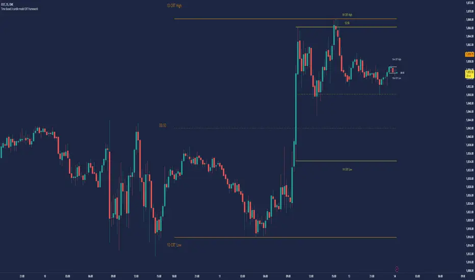
Time Based 3 Candle Model CRT FrameworkThe 3 Candle Model Overview:
The 3 Candle Model serves as a sophisticated framework for traders to navigate the complexities of financial markets, particularly within futures and forex trading. This guide not only elaborates on the model's key features but also emphasizes its originality and practical usefulness in the TradingView community. The core principle of the 3 Candle Model revolves around understanding how candle patterns can represent significant price ranges, offering valuable insights into potential market movements. By integrating the model with other critical trading concepts such as the Power of Three (PO3), Open-High-Low-Close (OHLC), and Turtle Soup setups, traders can enhance their ability to identify high-probability trades and achieve better trading outcomes.
Indicator includes:
3 Customizable Timeframe choices to fractally frame 3 candle models for precision
Live Timers for each timeframe to always be aware of the models timing
Parent Candle tracking on every preffered timeframe until new models parent candle is printed
Key Features of the 3 Candle Model
The 3 Candle Model primarily utilizes a three-candle structure, where the first candle establishes a price range, the second candle may act as a confirmation (often termed a "turtle soup"), and the third candle provides the breakout or continuation. This structure is pivotal in determining entry and exit points for trades, ensuring that each trading decision is backed by solid price action analysis.
OHLC Principle:
The Open-High-Low-Close (OHLC) concept is integral to the 3 Candle Model, allowing traders to analyze price action more effectively. Understanding the relationship between these four price points helps traders gauge market sentiment and potential reversals. By incorporating OHLC into the model, traders can develop a deeper understanding of market structure and its implications for future price movements.
Delivery States:
The 3 Candle Model emphasizes the importance of delivery states, which refer to the market's phase during specific time frames. Recognizing these states aids traders in determining the appropriate conditions for entering trades, particularly when combined with the power of three and candle range patterns. This understanding is crucial for positioning trades in alignment with market momentum.
High Probability Setups:
By aligning the 3 Candle Model with inside bar setups, traders can optimize their strategies for high-probability outcomes. This approach capitalizes on the inherent fractal nature of price movements, where previous patterns repeat at different scales. The combination of the model and inside bar setups enhances the trader's toolkit, allowing for more strategic trade placements.
Turtle Soup Formation:
The 3 Candle Model intricately connects with the Turtle Soup concept, which focuses on false breakouts. Identifying these formations at critical levels enhances the trader's ability to anticipate reversals or continuation patterns. The timing of these setups, particularly during specified times like 3:00 AM, 6:00 AM, 9:00 AM, and 1:00 PM, is crucial for maximizing trade success.
Using the 3 Candle Model in Trading
Integration with PO3:
The Power of Three (PO3) is a fundamental aspect of the 3 Candle Model that emphasizes the significance of three distinct stages of price delivery. Traders can leverage this principle by observing the initial range, confirming patterns, and executing trades during the third phase, leading to higher risk-to-reward ratios. This three-stage approach enhances a trader's ability to make informed decisions based on market behavior.
Targeting Midpoints:
Successful application of the 3 Candle Model involves targeting the midpoints of identified ranges. This practice not only provides strategic entry points but also enhances the probability of reaching desired profit levels. By targeting these midpoints, traders can refine their exit strategies and manage risk more effectively.
Aligning with Market Timing:
Timing is everything in trading. By synchronizing the 3 Candle Model setups with the aforementioned key timeframes, traders can better position themselves to exploit market dynamics. This alignment also facilitates the identification of high-quality trades that exhibit strong potential for profitability.
Prioritizing A+ Setups:
By focusing on the 3 Candle Model and its associated concepts, traders can prioritize A+ setups that exhibit a strong alignment of factors. This methodical approach enhances the quality of trades taken, leading to improved overall performance. By cultivating a strategy centered on high-probability setups, traders can maximize their return on investment.
Ensuring Originality and Usefulness
To meet the TradingView community guidelines, it is essential that this script is both original and useful. The 3 Candle Model, in its essence, is designed to provide traders with a unique perspective on market movements, free from generic or rehashed strategies. This tool integrates unique interpretations of the three-candle model and the associated strategies that are distinctly articulated and innovative.
Practical Applications: there are many practical applications of the 3 Candle Model in various trading contexts. This model in conjunction with other strategies to cultivate high-probability trade setups that can enhance performance across diverse market conditions.
Educational Value: This script is crafted with educational value in mind, providing insights that extend beyond mere trading signals. It encourages users to develop a deeper understanding of market mechanics and the interplay between price action, time, and trader psychology.
Conclusion
The 3 Candle Model provides a comprehensive framework for traders to enhance their trading strategies in the futures and forex markets. By understanding and applying the principles of this model alongside the Power of Three, OHLC concepts, and Turtle Soup formations, traders can significantly improve their ability to identify high-probability trades. The emphasis on timing, delivery states, and alignment of ranges ensures that traders are well-equipped to navigate the complexities of market movements, ultimately leading to more consistent and rewarding trading outcomes.
As trading involves risk, it is essential for traders to utilize these principles judiciously and maintain a disciplined approach to their trading strategies. By adhering to the TradingView community guidelines and emphasizing originality, usefulness, and detailed descriptions, this 3 Candle Model script stands as a valuable resource for traders seeking to refine their skills and achieve greater success in the financial markets.
Through this detailed exploration of the 3 Candle Model, traders will not only learn to recognize and exploit key patterns in price action but also appreciate the interconnectedness of various trading strategies that can significantly enhance their performance and profitability.
COT INDEX v2The **Commitment of Traders (COT)** report is a valuable tool for analyzing market sentiment, providing insight into the positions of futures traders at the close of the Tuesday trading session. Prepared by the Commodity Futures Trading Commission (CFTC), the report is published every Friday at 3:30 p.m. Eastern Time, and the data is freely available on the CFTC website.
Traders are categorized into three groups: **Commercial Traders**, **Non-Commercial Traders** (large speculators), and **Nonreportable** (small speculators). This information can be applied to charts to visualize the direction of the positions held by major market participants and to receive key COT signals.
The **COT index** ranges from 0% to 100%, reflecting market sentiment over the past 26 weeks. Extreme values, below 25% or above 75%, represent bearish or bullish sentiment, respectively. However, it is important to note that the COT index is not a timing tool but rather an indicator of the overall sentiment of major market players.
For a more tailored analysis, you can adjust the period for index calculation, customize chart styles, and highlight extreme areas.

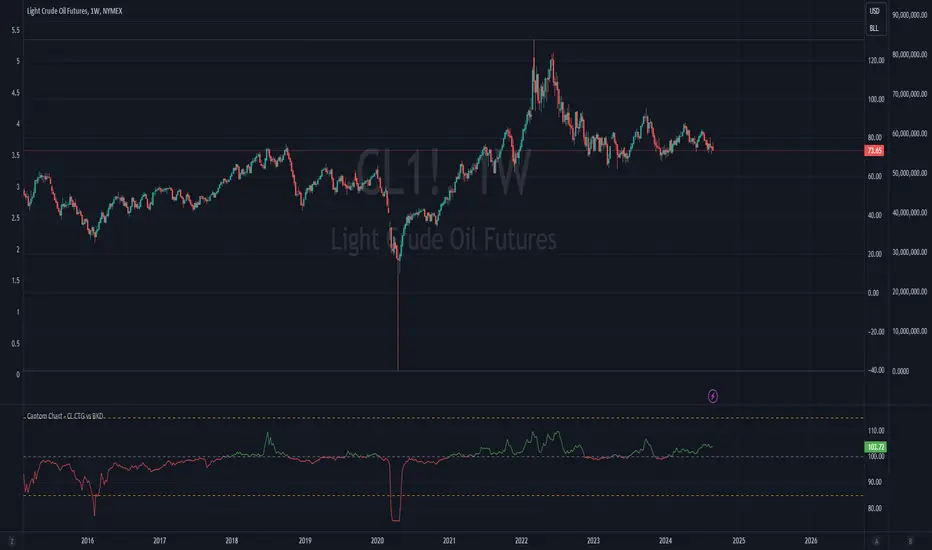
Cantom Chart - CL CTG vs BKDEnglish : This Pine Script indicator, named "Cantom Chart - CL CTG vs BKD," uniquely analyzes the immediate state of oil futures contracts to determine if they are in contango or backwardation. The script uses the price ratio between the nearest (CL1) and the next nearest (CL2) NYMEX crude oil futures contracts. It multiplies this ratio by 100 for clarity and scales fluctuations for enhanced visibility.
Key Features:
Dynamic Ratio Calculation: Computes the ratio (CL1/CL2 * 100) to determine the immediate market state.
Market State Interpretation: A ratio above 100 indicates backwardation, suggesting higher demand than supply, while a ratio below 100 indicates contango, suggesting higher supply than demand.
Volatility Adjustment: Amplifies market state changes by tripling the deviation from the baseline of 100, making it easier to observe subtle shifts.
Anomaly Detection: Caps the adjusted ratio at 125 for highs and 75 for lows, maintaining these limits until the ratio returns to normal levels.
Usage: This indicator is especially useful for traders analyzing supply-demand dynamics and inflationary pressures in the oil market. To apply it, simply add the script to your TradingView chart and adjust the 'Lower Threshold' and 'Upper Threshold' lines as needed based on your trading strategy.
-----
日本語 : この「Cantom Chart - CL CTG vs BKD」Pine Scriptインジケーターは、直近の原油先物契約がコンタンゴまたはバックワーデーションにあるかを特定するための独自の分析を提供します。最近の(CL1)と次の(CL2)NYMEX原油先物契約間の価格比を使用し、この比率に100を掛けて明確性を高め、変動の視認性を向上させます。
主要機能:
動的比率計算: 市場の即時状態を判断するために比率(CL1/CL2 * 100)を計算します。
市場状態の解釈: 比率が100を超える場合はバックワーデーション(需要が供給を上回る)、100未満の場合はコンタンゴ(供給が需要を上回る)を示します。
変動調整: 基準値100からの偏差を3倍にして、微妙な変化を容易に観察できるようにします。
異常値検出: 調整された比率を高値で125、低値で75に制限し、通常のレベルに戻るまでこれらの限界を維持します。
使用方法: このインジケーターは、原油市場における需給ダイナミクスとインフレ圧力を分析するトレーダーにとって特に有用です。使用するには、このスクリプトをTradingViewチャートに追加し、トレーディング戦略に基づいて「Lower Threshold」と「Upper Threshold」のラインを必要に応じて調整します。
Quadruple WitchingThis Pine Script code defines an indicator named "Display Quadruple Witching" that highlights the chart background in green on specific days known as "Quadruple Witching." Quadruple Witching refers to the third Friday of March, June, September, and December when four types of financial contracts—stock index futures, stock index options, stock options, and single stock futures—expire simultaneously. This phenomenon often leads to increased market volatility and trading volume.
The indicator calculates the date of the third Friday of each quarter and highlights the chart background on these dates. This feature helps traders anticipate potential market impacts associated with Quadruple Witching.
Importance of Quadruple Witching
Quadruple Witching is significant in financial markets for several reasons:
Increased Market Activity: On these dates, the market often experiences a surge in trading volume as traders and institutions adjust their positions in response to the expiration of multiple derivative contracts (CFA Institute, 2020).
Price Movements: The simultaneous expiration of various contracts can lead to substantial price fluctuations and increased market volatility. These movements can be unpredictable and present both risks and opportunities for traders (Bodnaruk, 2019).
Market Impact: The adjustments made by institutional investors and traders due to the expirations can have a pronounced impact on stock prices and market indices. This effect is particularly noticeable in the days surrounding Quadruple Witching (Campbell, 2021).
References
CFA Institute. (2020). The Impact of Quadruple Witching on Financial Markets. CFA Institute Research Foundation. Retrieved from CFA Institute.
Bodnaruk, A. (2019). The Effect of Option Expiration on Stock Prices. Journal of Financial Economics, 131(1), 45-64. doi:10.1016/j.jfineco.2018.08.004
Campbell, J. Y. (2021). The Behaviour of Stock Prices Around Expiration Dates. Journal of Financial Economics, 141(2), 577-600. doi:10.1016/j.jfineco.2021.01.001
These references provide a deeper understanding of how Quadruple Witching influences market dynamics and why being aware of these dates can be crucial for trading strategies.

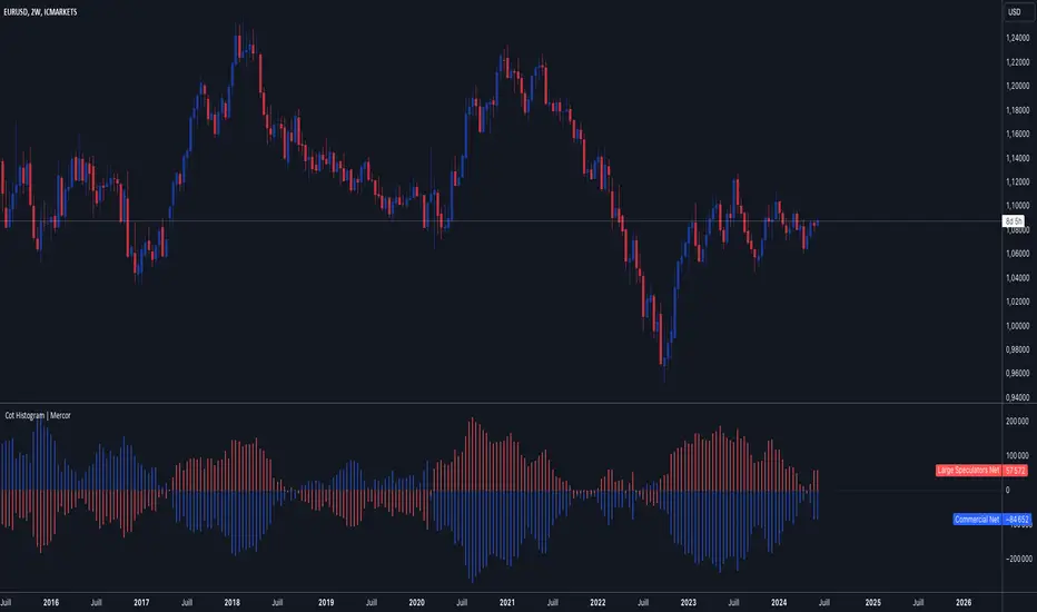
Cot Histogram | MercorCot Histogram | Mercor
Overview:
The Cot Histogram | Mercor indicator provides a comprehensive visualization of the Commitment of Traders (COT) report data using bar charts. This indicator is designed to help traders analyze the positions held by commercial traders and large speculators in various markets. By representing the data as histograms, traders can easily interpret the long and short positions, as well as the net positions of these market participants.
Originality:
What sets the Cot Histogram | Mercor indicator apart is its unique approach to visualizing COT data using bar charts instead of traditional line charts. This method offers a clearer representation of the data, making it easier for traders to spot trends and changes in market sentiment. Additionally, the indicator allows for customization of colors and bar widths, providing a tailored experience for each user.
Features:
Show Shorts as Negative Numbers: This option allows users to display short positions as negative values, providing a more intuitive visualization.
Invert Colors: Users can invert the default colors for long and short positions, enabling better contrast and visual preference.
Bar Width: Adjust the width of the histogram bars to suit personal preferences and chart aesthetics.
Concepts Underlying the Calculations:
The Commitment of Traders (COT) report is a weekly publication by the Commodity Futures Trading Commission (CFTC) that provides a breakdown of the open interest positions of market participants in futures markets. This indicator focuses on two main categories of traders:
Commercial Traders: These are entities involved in the production, processing, or merchandising of a commodity. Their positions are typically hedging-oriented.
Large Speculators: These include institutional investors, hedge funds, and other entities that take positions based on market trends and expectations, often for speculative purposes.
The indicator calculates and plots the following metrics:
Commercial Long: The number of long positions held by commercial traders.
Commercial Short: The number of short positions held by commercial traders.
Commercial Net: The difference between commercial long and short positions.
Large Speculators Long: The number of long positions held by large speculators.
Large Speculators Short: The number of short positions held by large speculators.
Large Speculators Net: The difference between long and short positions of large speculators.
How to Use:
Load the Indicator: Add the Cot Histogram | Mercor indicator to your TradingView chart.
Customize Settings: Adjust the settings according to your preferences:
Enable or disable the "Show Shorts as Negative Numbers" option.
Invert the colors if needed.
Adjust the bar width for better visual representation.
Interpret the Data: Use the histograms to analyze the market positions:
Commercial Long and Short: Observe the positions held by commercial traders. Increasing long positions may indicate hedging against potential price increases, while increasing short positions may suggest hedging against potential price decreases.
Large Speculators Long and Short: Monitor the positions of large speculators to gauge market sentiment. A rise in long positions by large speculators often indicates bullish sentiment, while a rise in short positions suggests bearish sentiment.
Net Positions: The net positions provide a clearer picture of the overall stance of commercial traders and large speculators.
Example:
If you notice that commercial traders are increasing their long positions while large speculators are increasing their short positions, it may indicate a divergence in market expectations between hedgers and speculators. This could be a signal to further investigate potential market reversals or confirm existing trends.
By leveraging the Cot Histogram | Mercor indicator, traders can gain valuable insights into market dynamics, improve their trading strategies, and make more informed decisions. Whether you are a long-term investor or a short-term trader, understanding the positions of different market participants can provide a significant edge in the markets.
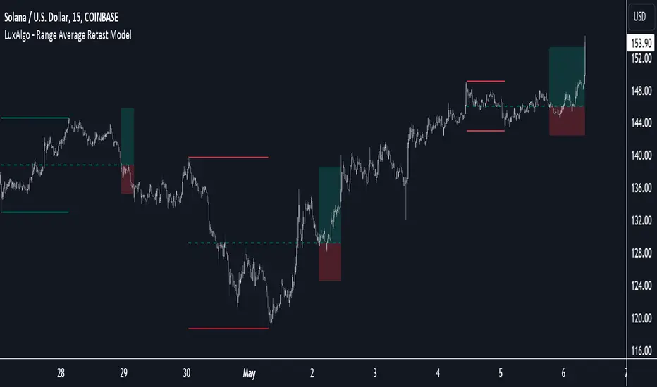
Range Average Retest Model [LuxAlgo]The Range Average Retest Model tool highlights setups from the range average retest entry model, a model using the retest of the average between two opposite swing points as an entry.
This tool uses long-term volatility coupled with user-defined multipliers to filter out swing areas and set take profit and stop loss levels for all trades.
Key features include:
Draw up to 165 swing areas and their associated trades
Filter out swing areas using Pivot Length , Selection Mode and Threshold parameters
Filter out trades with Maximum Distance and Minimum Distance parameters
Enable or disable swing areas and select default colors
Enable or disable overlapping trades and change the default colors for Take Profit and Stop Loss zones
🔶 USAGE
The "Range Average Retest Model" is an entry model that enters a position when the price retests the average made between two swing points. Users can determine the period of the detected swing points from the "Pivot Length" setting.
The conditions for long or short trades, regardless of whether the swing area is bullish or bearish, are as follows:
Long positions: the current bar close is below the swing area average and the last bar close was above it.
Short positions: the current bar close is above the swing area average price and the last bar close was below it.
Each trade is displayed on the chart with a line connecting it to its swing area highlighting the range average, a green area for the take profit, and a red area for the stop loss.
Both the Take Profit and Stop Loss levels are calculated by applying your own multiplier in the settings panel to the long-term volatility measure, in this case, the average true range over the last 200 bars.
Trades will remain open until they reach either the Stop Loss or Take Profit price levels.
🔹 Filtering Swing Areas
The daily chart of the Nasdaq-100 futures (NQ) with pivot length 2 and bullish selection mode: it only detects bullish swing areas, but they are smaller and more numerous.
Traders can manipulate the behavior of the swing areas from the settings panel.
The Selection mode will filter areas by bias: it will detect bullish areas, bearish areas, or both.
The Threshold parameter is applied to the long-term volatility to filter out areas where the average prices are too close together; the higher the value, the greater the difference between the average prices must be.
🔹 Trades
3-minute chart of the Nasdaq-100 futures (NQ) with pivot length 5, bearish selection mode maximum distance 4, and stop loss 2: many trades detected with very asymmetric risk/reward.
The behavior of the trades is also manipulated from the settings panel.
The maximum and minimum distance parameters specify the number of bars a trade must be away from a swing area.
The Take Profit and Stop Loss parameters are applied to the long-term volatility to obtain their respective price levels.
🔹 Overlapping Trades
Same chart as before, but with overlapping trades: messy, right?
By default the tool does not show overlapping trades, this allows for a cleaner chart.
In the settings panel traders can enable overlapping mode, in which case the tool will show all available trades.
Traders must be aware that the chart can be very crowded.
🔶 SETTINGS
🔹 Swings
Pivot Length: How many bars are used to confirm a swing point. The larger this parameter is, the larger and fewer swing areas will be detected.
Selection Mode: Swing area detection mode, detect only bullish swings, only bearish swings, or both.
Threshold: Swing area comparator. This threshold is multiplied by a measure of volatility (average true range over the last 200 bars), for a new swing area to be detected it must have an average level that is sufficiently distant from the average level of any untouched swing area, this parameter controls that distance.
🔹 Trades
Maximum distance: Maximum distance allowed between a swing area and a trade.
Minimum distance: Minimum distance allowed between a swing area and a trade.
Take profit: The size of the take profit - this threshold is multiplied by a measure of volatility (the average true range over the last 200 bars).
Stop loss: The size of the stop-loss: this threshold is multiplied by a measure of volatility (the average true range over the last 200 bars).
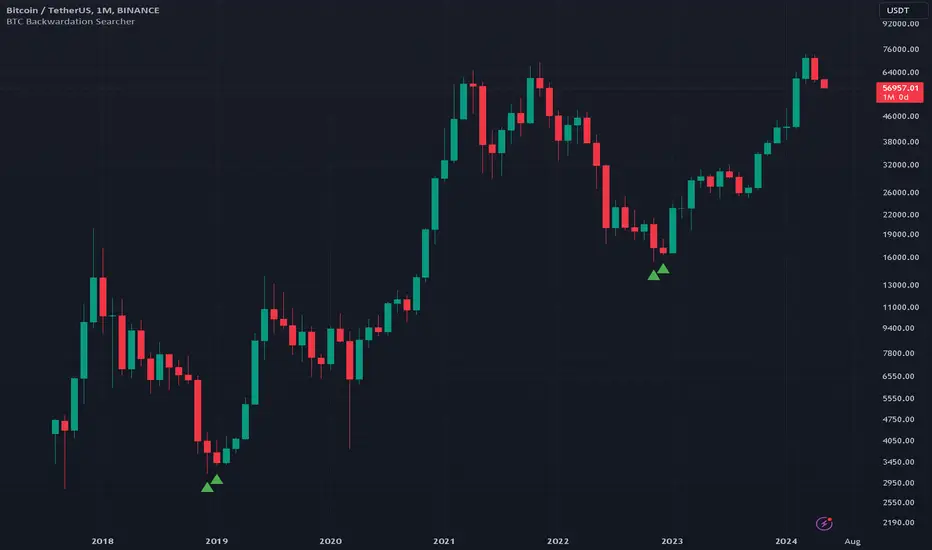
BTC Backwardation SearcherThis Pine Script code is a custom indicator named "BTC Backwardation Searcher" designed for the TradingView platform. The indicator aims to identify and visualize the price difference between two Bitcoin futures contracts: CME:BTC1! and CME:BTC2!.
Here's a breakdown of the code:
1. The script fetches the daily close prices of CME:BTC1! and CME:BTC2! using the security() function.
2. It calculates the percentage price difference between the two contracts using the formula: (btc1Price - btc2Price) / btc2Price * 100.
3. The script also calculates the price difference for the previous two days (2 days ago and 3 days ago) using the same formula.
4. Two conditions are defined:
(1) dailyGreenCondition: If the price difference is greater than or equal to 0.3% for three
consecutive days, including the current day and the previous two days.
(2) dailyRedCondition(commented): If the price difference is less than or equal to -1% for three consecutive days, including the current day and the previous two days.
(I commented it out because I don't think it's useful.)
5. The plotshape() function is used to display green triangles on the chart when the dailyGreenCondition is met, and red triangles when the dailyRedCondition is met. These triangles are displayed on the daily, weekly, and monthly timeframes.
The purpose of this indicator is to help traders identify potential trading opportunities based on the price difference between the two Bitcoin futures contracts. The green triangles suggest a bullish scenario where CME:BTC1! is significantly higher than CME:BTC2!, while the red triangles indicate a bearish scenario where CME:BTC2! is significantly lower than CME:BTC1!.
However, it's important to note that this indicator should be used in conjunction with other technical analysis tools and fundamental analysis. Traders should also consider their risk tolerance, investment goals, and market conditions before making any trading decisions based on this indicator.
Open interest buildup & Session Open high-lowThis indicator is to be used on srcipts in Futures Segment.
1. It visually displays in tabular format the change in open interest and the change in price compared to the previous day.
2. It also displays the scenario where open price of session is near high price of session or low price of session, indicating a emergence of strong sellers or strong buyers from start of session respectively.
3. A positive change in open interest and a positive change in price is denoted by a long buildup and open price near low price is an additional confirmation for a probable long scenario in the script.
4. A positive change in open interest and a negative change in price is denoted by a short buildup and open price near high price is and additional confirmation for a probable short scenario in the script.
Key features of the indicator include:
Override Symbol Input: Traders can override the default symbol and input their preferred symbol for analysis.
Open Interest Data: The indicator retrieves open interest data for the selected symbol and time frame, facilitating analysis based on changes in open interest.
Dashboard: The indicator features a customizable dashboard that displays key information such as build-up conditions, OI change, and price change.
Build-Up Conditions: The indicator identifies long build-up and short build-up scenarios based on user-defined thresholds for OI change and price change percentages.
Customization Options: Traders have the flexibility to customize various aspects of the indicator, including colors for long build-up, short build-up, positive OI change, negative OI change, positive price change, and negative price change.
Label Plots: Buy and sell labels are plotted on the chart to highlight potential trading opportunities. Traders can customize the colors and text colors of these labels based on their preferences.
Overall, the indicator offers traders a comprehensive tool for analyzing price movements and open interest changes, helping them make informed trading decisions in the futures segment.

Custom spreadThis indictor allows you to plot the spread over an arbitrary period, which can be especially useful for futures and other instruments.
Inputs:
Expression : symbols for calculation and arithmetic operation
Period: from to period and timeframe
The output will show bars for the given period
Particularly useful for comparing two selected contracts on two futures

Murrey Math
The Murrey Math indicator is a set of horizontal price levels, calculated from an algorithm developed by stock trader T.J. Murray.
The main concept behind Murrey Math is that prices tend to react and rotate at specific price levels. These levels are calculated by dividing the price range into fixed segments called "ranges", usually using a number of 8, 16, 32, 64, 128 or 256.
Murrey Math levels are calculated as follows:
1. A particular price range is taken, for example, 128.
2. Divide the current price by the range (128 in this example).
3. The result is rounded to the nearest whole number.
4. Multiply that whole number by the original range (128).
This results in the Murrey Math level closest to the current price. More Murrey levels are calculated and drawn by adding and subtracting multiples of the range to the initially calculated level.
Traders use Murrey Math levels as areas of possible support and resistance as it is believed that prices tend to react and pivot at these levels. They are also used to identify price patterns and possible entry and exit points in trading.
The Murrey Math indicator itself simply calculates and draws these horizontal levels on the price chart, allowing traders to easily visualize them and use them in their technical analysis.
HOW TO USE THIS INDICATOR?
To use the Murrey Math indicator effectively, here are some tips:
1. Choose the appropriate Murrey Math range : The Murrey Math range input (128 by default in the provided code) determines the spacing between the levels. Common ranges used are 8, 16, 32, 64, 128, and 256. A smaller range will give you more levels, while a larger range will give you fewer levels. Choose a range that suits the volatility and trading timeframe you're working with.
2. Identify potential support and resistance levels: The horizontal lines drawn by the indicator represent potential support and resistance levels based on the Murrey Math calculation. Prices often react or reverse at these levels, so they can be used to spot areas of interest for entries and exits.
3. Look for price reactions at the levels: Watch for price action like rejections, bounces, or breakouts at the Murrey Math levels. These reactions can signal potential trend continuation or reversal setups.
4. Trail stop-loss orders: You can place stop-loss orders just below/above the nearest Murrey Math level to manage risk if the price moves against your trade.
5. Set targets at future levels: Project potential profit targets by looking at upcoming Murrey Math levels in the direction of the trend.
7. Adjust range as needed: If prices are consistently breaking through levels without reacting, try adjusting the range input to a different value to see if it provides better levels.
In which asset can this indicator perform better?
The Murrey Math indicator can potentially perform well on any liquid financial asset that exhibits some degree of mean-reversion or trading range behavior. However, it may be more suitable for certain asset classes or trading timeframes than others.
Here are some assets and scenarios where the Murrey Math indicator can potentially perform better:
1. Forex Markets: The foreign exchange market is known for its ranging and mean-reverting nature, especially on higher timeframes like the daily or weekly charts. The Murrey Math levels can help identify potential support and resistance levels within these trading ranges.
2. Futures Markets: Futures contracts, such as those for commodities (e.g., crude oil, gold, etc.) or equity indices, often exhibit trading ranges and mean-reversion trends. The Murrey Math indicator can be useful in identifying potential turning points within these ranges.
3. Stocks with Range-bound Behavior: Some stocks, particularly those of large-cap companies, can trade within well-defined ranges for extended periods. The Murrey Math levels can help identify the boundaries of these ranges and potential reversal points.
4. I ntraday Trading: The Murrey Math indicator may be more effective on lower timeframes (e.g., 1-hour, 30-minute, 15-minute) for intraday trading, as prices tend to respect support and resistance levels more closely within shorter time periods.
5. Trending Markets: While the Murrey Math indicator is primarily designed for range-bound markets, it can also be used in trending markets to identify potential pullback or continuation levels.
Historical Correlation [LuxAlgo]The Historical Correlation tool aims to provide the historical correlation coefficients of up to 10 pairs of user-defined tickers starting from a user-defined point in time.
Users can choose to display the historical values as lines or the most recent correlation values as a heat map.
🔶 USAGE
This tool provides historical correlation coefficients, the correlation coefficient between two assets highlight their linear relationship and is always within the range (-1, 1).
It is a simple and easy to use statistical tool, with the following interpretation:
Positive correlation (values close to +1.0): the two assets move in sync, they rise and fall at the same time.
Negative correlation (values close to -1.0): the two assets move in opposite directions: when one goes up, the other goes down and vice versa.
No correlation (values close to 0): the two assets move independently.
The user must confirm the selection of the anchor point in order for the tool to be executed; this can be done directly on the chart by clicking on any bar, or via the date field in the settings panel.
For the parameter Anchor period , the user can choose between the following values NONE, HOURLY, DAILY, WEEKLY, MONTHLY, QUARTERLY and YEARLY. If NONE is selected, there will be no resetting of the calculations, otherwise the calculations will start from the first bar of the new period.
There is a wide range of trading strategies that make use of correlation coefficients between assets, some examples are:
Pair Trading: Traders may wish to take advantage of divergences in the price movements of highly positively correlated assets; even highly positively correlated assets do not always move in the same direction; when assets with a correlation close to +1.0 diverge in their behavior, traders may see this as an opportunity to buy one and sell the other in the expectation that the assets will return to the likely same price behavior.
Sector rotation: Traders may want to favor some sectors that are expected to perform in the next cycle, tracking the correlation between different sectors and between the sector and the overall market.
Diversification: Traders can aim to have a diversified portfolio of uncorrelated assets. From a risk management perspective, it is useful to know the correlation between the assets in your portfolio, if you hold equal positions in positively correlated assets, your risk is tilted in the same direction, so if the assets move against you, your risk is doubled. You can avoid this increased risk by choosing uncorrelated assets so that they move independently.
Hedging: Traders may want to hedge positions with correlated assets, from a hedging perspective, if you are long an asset, you can hedge going long a negative correlated asset or going short a positive correlated asset.
Traders generally need to develop awareness, a key point is to be aware of the relationships between the assets we hold or trade, the historical correlation is an invaluable tool in our arsenal which allows us to make better informed decisions.
On this chart we have an example of historical correlations for several futures markets.
We can clearly see how positively correlated the Nasdaq100 and Dow30 are with the SP500 over the whole period, or how the correlation between the Euro and the SP500 falls from almost +85% to almost -4% since 2021.
As we can see, correlations, like everything else in the market, are not static and vary over time depending on many factors, from macro to technical and everything in between.
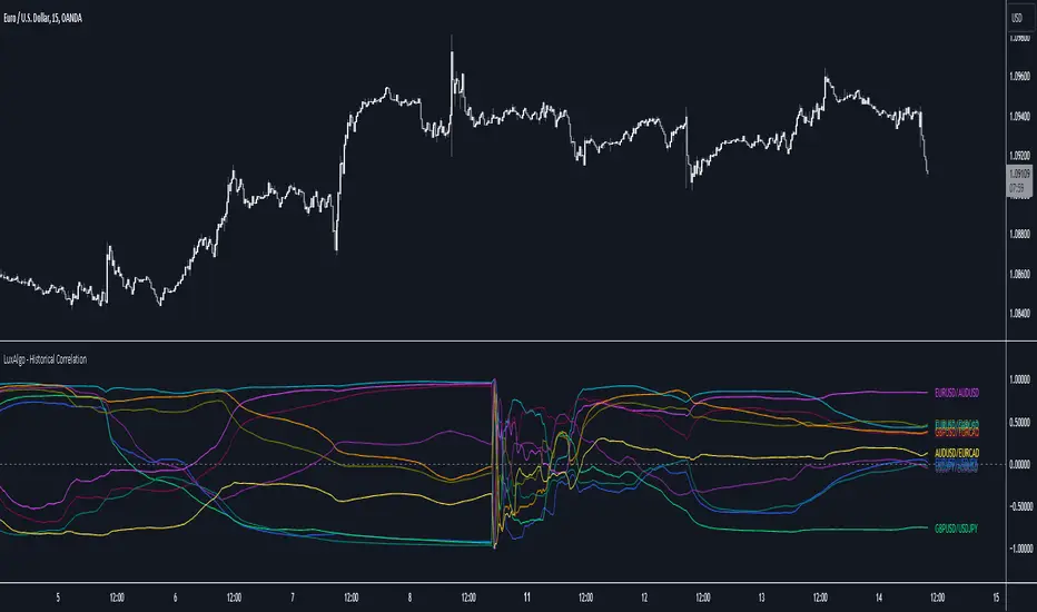
🔹 Heatmap
The chart above shows the tool with the default settings and the Drawing Mode set to 'HEATMAP'.
We can see the current correlation between the assets, in this case the FX pairs.
The highest positive correlation is +90% (+0.90) between EURUSD and GBPUSD.
The highest negative correlation is -78% (-0.78) between EURUSD and USDJPY.
The pair with no correlation is AUDUSD and EURCAD with 1% (0.01)
On the above chart we can see the current correlations for the futures markets.
Currently, the assets that are less correlated to the SP500 are NaturalGas and the Euro, the more positive correlations are Nasdaq100 and Dow20, and the more negative correlations are the Yen, Treasury Bonds and 10-Year Notes.
🔶 DETAILS
🔹 Anchor Period
This chart shows the standard FX correlations with the Anchor Period set to `MONTHLY`.
We can clearly see how the calculations restart with the new month, in this case we can clearly see the differences between the correlations from month to month.
Let us look at the correlation coefficient between GBPUSD and USDJPY
In January, their correlation started at close to -100%, rose to close to +50%, only to fall to close to 0% and remain there for the second half of the month.
In February it was -90% in the first few days of the month and is now around -57%.
And between AUDUSD and EURCAD
Last month their correlation was negative for most of the month, reaching -70% and ending around -14%.
This month their correlation has never gone below +21% and at the time of writing is close to +53%.
🔶 SETTINGS
Anchor point: Starting point from which the tool is executed
Anchor period: At the beginning of each new period, the tool will reset the calculations
Pairs from 1 to 10: For each pair of tickers, you can: enable/disable the pair, select the color and specify the two tickers from which you wish to obtain the correlation
🔹 Style
Drawing Mode: Output style, `LINES` will show the historical correlations as lines, `HEATMAP` will show the current correlations with a color gradient from green for correlations near 1 to red for correlations near -1.
Commitments of Traders Report [Advanced]This indicator displays the Commitment of Traders (COT) report data in a clear, table format similar to an Excel spreadsheet, with additional functionalities to analyze open interest and position changes. The COT report, published weekly by the Commodity Futures Trading Commission (CFTC), provides valuable insights into market sentiment by revealing the positioning of various trader categories.
Display:
Release Date: When the data was released.
Open Interest: Shows the total number of open contracts for the underlying instrument held by selected trader category.
Net Contracts: Shows the difference between long and short positions for selected trader category.
Long/Short OI: Displays the long and short positions held by selected trader category.
Change in Long/Short OI: Displays the change in long and short positions since the previous reporting period. This can highlight buying or selling pressure.
Long & Short Percentage: Displays the percentage of total long and short positions held by each category.
Trader Categories (Configurable)
Commercials: Hedgers who use futures contracts to manage risk associated with their underlying business (e.g., producers, consumers).
Non-Commercials (Large Speculators): Speculative traders with large positions who aim to profit from price movements (e.g., hedge funds, investment banks).
Non-Reportable (Small Speculators/Retail Traders): Smaller traders with positions below the CFTC reporting thresholds.
CFTC Code: If the indicator fails to retrieve data, you can manually enter the CFTC code for the specific instrument. The code for instrument can be found on CFTC's website.
Using the Indicator Effectively
Market Sentiment Gauge: Analyze the positioning of each trader category to gauge overall market sentiment.
High net longs by commercials might indicate a bullish outlook, while high net shorts could suggest bearish sentiment.
Changes in open interest and long/short positions can provide additional insights into buying and selling pressure.
Trend Confirmation: Don't rely solely on COT data for trade signals. Use it alongside price action and other technical indicators for confirmation.
Identify Potential Turning Points: Extreme readings in COT data, combined with significant changes in open interest or positioning, might precede trend reversals, but exercise caution and combine with other analysis tools.
Disclaimer
Remember, the COT report is just one piece of the puzzle. It should not be used for making isolated trading decisions. Consider incorporating it into a comprehensive trading strategy that factors in other technical and fundamental analysis.
Credit
A big shoutout to Nick from Transparent FX ! His expertise and thoughtful analysis have been a major inspiration in developing this COT Report indicator. To know more about this indicator and how to use it, be sure to check out his work.

Short Interest Tracker [SS]This is a simple indicator that is designed to provide you with a synopsis of short interest on the daily, weekly and monthly timeframes.
How it works:
It pulls FINRA ticker data on short volume for whichever ticker you are on. It works with all tickers provided they are listed on FINRA (which is all tickers).
It will not work with futures, for futures, you would want to use a COT-based indicator, but for indices and equities, this indicator will provide you with the short volume information.
What it shows:
It breaks short volume down into current short volume, the 14-period SMA of short volume over the day, week and month, it also provides you with a short volume to SMA ratio. This is Short Volume divided by the SMA. Anything below 1 is good, it means short interest is low. Anything above 1 is not good, it means that short volume is above the SMA.
It also will show you the weekly, daily and monthly short volume change.
And last but not least, it will tell you whether short interest is falling, rising or steady. How it does this is by tracking whether the SMA is increasing, decreasing or stagnant.
Customization:
You can customize the SMA length and the assessment of whether short volume is increasing or decreasing. The default SMA length is 14 and the default assessment of rising/falling short volume is 4. This means, short volume has to rise or fall over a 4-period timeframe for it to register. So on the week, if it displays short volume increasing, it means that, over the past 4 weeks, the sma has steadily risen. Inverse if it decreases. If you want it to be more sensitive, you can reduce it to 2 or 3. If you want it to be more strict, you can increase it to 5 or 6.
NOTE:
If the volume information for a ticker is not available, it will return a runtime error indicating as such.
And that's the indicator!
I wanted something similar to COT data for equities and indices, so this was my attempt to bridge that gap.
Hope you enjoy and find it useful! Leave your suggestions below.
Take care everyone!

Cross Correlation [Kioseff Trading]Hello!
This script "Cross Correlation" calculates up to ~10,000 lag-symbol pair cross correlation values simultaneously!
Cross correlation calculation for 20 symbols simultaneously
+/- Lag Range is theoretically infinite (configurable min/max)
Practically, calculate up to 10000 lag-symbol pairs
Results can be sorted by greatest absolute difference or greatest sum
Ability to "isolate" the symbol on your chart and check for cross correlation against a list of symbols
Script defaults to stock pairs when on a stock, Forex pairs when on a Forex pair, crypto when on a crypto coin, futures when on a futures contract.
A custom symbol list can be used for cross correlation checking
Can check any number of available historical data points for cross correlation
Practical Assessment
Ideally, we can calculate cross correlation to determine if, in a list of assets, any of the assets frequently lead or lag one another.
Example
Say we are comparing the log returns for the previous 10 days for SPY and XLU.
*A single time-interval corresponds to the timeframe of your chart i.e. 1-minute chart = 1-minute time interval. We're using days for this example.
(Example Results)
A lag value (k) +/-3 is used.
The cross correlation (normalized) for k = +3 is -0.787
The cross correlation (normalized) for k = -3 is 0.216
A positive "k" value indicates the correlation when Asset A (SPY) leads Asset B (XLU)
A negative "k" value indicates the correlation when Asset B (XLU) leads Asset A (SPY)
A normalized cross correlation of -0.787 for k = +3 indicates an "adequately strong" negative relationship when SPY leads XLU by 3 days.
When SPY increases or decreases - XLU frequently moves in the opposite direction 3 days later.
A cross correlation value of 0.216 at k = −3 indicates a "weak" positive correlation when XLU leads SPY by 3 days.
There's a slight tendency for SPY to move in the same direction as XLU 3 days later.
After the cross-correlation score is normalized it will fall between -1 and 1.
A cross-correlation score of 1 indicates a perfect directional relationship between asset A and asset B at the corresponding lag (k).
A cross correlation of -1 indicates a perfect inverse relationship between asset A and asset B at the corresponding lag (k).
A cross correlation of 0 indicates no correlation at the corresponding lag (k).
The image above shows the primary usage for the script!
The image above further explains the data points located in the table!
The image above shows the script "isolating" the symbol on my chart and checking the cross correlation between the symbol and a list of symbols!
Wrapping Up
With this information, hopefully you can find some meaningful lead-lag relationships amongst assets!
Thank you for checking this out (:

COT TFF Data (S&P_500_CONSOLIDATED)Commitment of Traders - Traders in Financial Futures (Futures and Options)
Custom python script is used to create the Pinescript strings from a spreadsheet containing the dates + net positions. Data is then input manually in Pinescript (can only fit 4-5 years of data).
This data set is from the: S&P_500_CONSOLIDATED
Source: cftc.gov

COT TFF Data (VIX_FUTURES)Commitment of Traders - Traders in Financial Futures (Futures and Options)
Custom python script is used to create the Pinescript strings from a spreadsheet containing the dates + net positions. Data is then input manually in Pinescript (can only fit 4-5 years of data).
This data set is from the: VIX_FUTURES
Source: cftc.gov

[blackcat] L1 Stella Osoba Donchian ChannelsLevel 1
Background
On Jul, 2023, Stella Osoba proposed a price channel idea in the article of “Using Price Channels”.
Function
In Stella Osoba's article "Using Price Channels" in the 2023 bonus issue, author Stella Osoba describes why many analysis techniques are based on the concept of price channels. In her explanation of the Donchian channels, she explains that they are used to identify the trend and that the prices for the last period are not included in the calculations. I rewrote this idea in the PINE version presented here, allowing the user to optionally include the most recent period. To not include the most recent period, set the IncludeRecentPeriod input to false.
Richard Donchian, a futures trader, created the Donchian Channel as a trend indicator. He was later dubbed the "father of trend following." Several trading methods based on Donchian channels have been established, but day traders can create their own as the indicator is versatile and can be interpreted in different ways. The renowned Turtle Traders also used a variation of the Donchian technique.
The Donchian Channel draws a line between the high and low price of an asset over a period of time, generally using candlesticks as a clock. Candlesticks are chart areas on charts that show the open, high, low, and close price and time frame of a particular stock. They owe their name to their shape. When the indicator is applied to a chart, the lines form a channel around the current price.
When day trading, Donchian channels are useful for highlighting trends and range periods. A third line can be added between the top and bottom lines if required. The upper and lower channel lines are averaged to form this center band. The indicator can be used on all timeframes, including one-minute and five-minute charts (where a bar forms every one or five minutes), and it can be used for forex, stock, futures, and options trading .
Remarks
Feedbacks are appreciated.