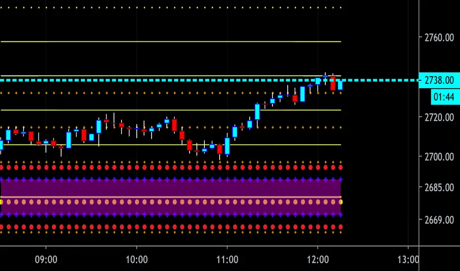
CBG Key Numbers v6Here is my opening range, key numbers indicator. It takes the Opening Range (5 minutes by default) and then plots the opening range and up to 7 extensions of that range above and below.
It's amazing how the OR is stamped up on the rest of the day's price movements.
2 strategies (at least) are to play the OR range breakout and to fade when price hits an extreme range.
You have total control over how you set up the various lines and colors.
If you start overlaying the trading day with the OR and it's extensions, you will see amazing patterns become clear. For example, the pump and reverse. This is where price pumps right out of the opening and then reverses later in the morning.
I have the opening price set to big circles as this is one of the most important reference points during the day.
Important: For some reason, the 9:30 am time Opening acts differently for equities and futures . For equities, you can set the time values to 0930. But for futures , to capture the Open at 9:30, you have to set the time values to start at 0830. I haven't been able to find a better solution but setting the times manually works. Make sure to set all the time values on the Options screen.
There is one more setting of interest. It is called IB Target Amount. This is a number above and below the opening range that I have observed price to hit whenever there's a breakout. This will allow you to predict a price target on breakouts. For SPY , I have found that price usually breaks out to at least 50 cents. On ES futures , it's 6 dollars. This can help you lock in 10% and 20% when trading options and is a great tool. That's why I have it so prominent in red. You will also see price return to this level during the day and act as support or resistance.
Please disregard the red and green shaded rectangles. They are my own support and resistance zones and TV wouldn't let me hide them from the picture. :-)
I mostly use this on a 5 minute chart but any timeframe will work.
"Futures" için komut dosyalarını ara
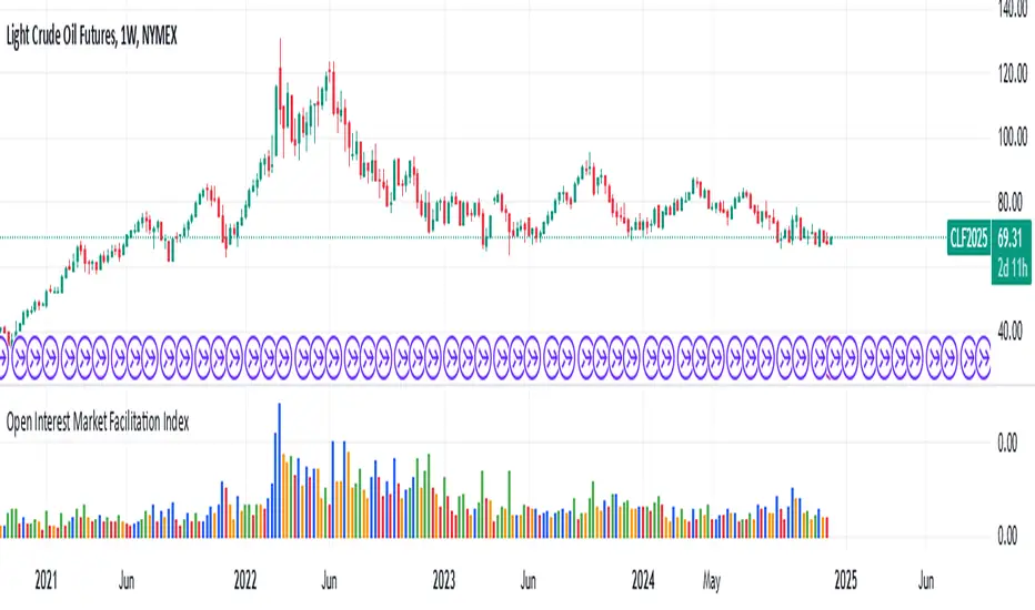
Open Interest Market Facilitation IndexOriginal script from ChartChampions :
Let's start.
This script was created by using Open Interest instead of Volume in the Market Facilitation Index.
Thus, it can make a difference in the Future and CFD Markets.
If your financial instrument is not from these markets, that is, if Open Interest is not used, you can choose Volume.
You can set "FUTURES" and "OTHERS" from the menu.
If you use the Open Interest (FUTURES) option in the menu on 1W bars and defined Future markets, it will not repaint.
This is the best use for Open Interests, as data is extracted from Quandl and CFTC COT reports are published once a week.
Color Change Rules :
In my version :
Green Bars = Green
Fade Bars = Orange
Fake Bars = Blue
Squat Bars = Red
To show the difference in the presentation, both the Futures option using Open Interest and the Others option using Volume were published to compare.
You can observe the difference.
Best regards.
plot CFTC COT disaggregated dataCFTC COT data is exported by quandl.com to tradingview
COT@quandl:
www.quandl.com
COT@tradingview
www.tradingview.com
How to use this script:
Select and load CFTC COT data for the commodity ticker in the chart
Will by default take current ticker, or allow to avvverride it with another
Traders' categories are those for commodities, not financial futs
Select And Configure :
-categories to be plotted
-Futures/Futures+Options
-by num_contracts/percent
-plot"Tot Spreads %" selection when also "Show as % of OI" selected
This script supercedes my other "MY_ CFTC GC/SI/CL (Disaggregated)" script

Delay Estimatorthis script can be used to adjust one of the free realtime tickers (such as SPX500, NAS100) to "look" like one of the delayed futures tickers (such as ES1!, NQ1!). This basically allows us to get an estimate of the realtime futures ticker price.
it uses bollinger bands to adjust the volatility and offset of the realtime ticker
it also provides a decimator to reduce the price into ticks, since futures often use 4 ticks per point

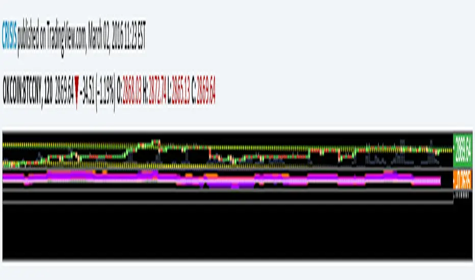
(CRISIS) BTC money flow oscilator V0.1Modified version of Ricado Santos' money flow oscilator.
now featuring 3 oscilators. Makes it easier to obseerve when dumps/pumps are targeting OKC futures contracts or just looking for divergences.
1x Aggregate of OKcoin:BTCCNY, Houbi:BTCCNY & Bitfinex:BTCUSD (Orange)
1X OKcoin 1 Week futures (pink)
1x OKcoin 3 Month futures (purple)
Herrick Payoff IndexThe Herrick Payoff Index is designed to show the amount of money flowing into or out of a futures contract. The Index uses open interest during its calculations, therefore, the security being analyzed must contain open interest.
The Herrick Payoff Index was developed by John Herrick.When the Herrick Payoff Index is above zero, it shows that money is flowing into the futures contract (which is bullish). When the Index is below zero, it shows that money is flowing out of the futures contract (which is bearish).
The interpretation of the Herrick Payoff Index involves looking for divergences between the Index and prices.

Stock ScreenerMissing great trade opportunities is annoying, and unless you have 12 screens or only trade one market, you are missing a lot of trades. To fix that, we created this stock screener so you get notified instantly of potential great trading conditions in real time, right on your chart.
You get notified of trading benchmarks being met by the value being displayed on the scanner as well as a color change so that it grabs your attention and makes you aware that you should take a look at the other market and look for a potential trade. It also has built in alerts so you can have an alert notification go off when any of your trading conditions are met instead of needing to watch the scanner for color changes.
The screener will change the ticker symbol background color to red green when price is above or below the previous daily range and above or below both VWAPs. This signals that the ticker is trending, which typically means it is a great time to trade that market and follow the trend.
This stock screener allows you to scan up to 10 different markets at the same time for various different conditions so you always know what is going on with your favorite trading symbols. If you want to scan more tickers, just add the indicator to your chart again and change the table position to the other side of the screen and update the tickers on the 2nd screener, allowing you to have 20 tickers at a time.
The scanner can be fully customized by changing the markets that it screens and turning on or off as many of them as you would like. You can also turn on or off any of the different data sets so that you only get information about trading conditions that matter to you.
The screener can provide data on any type of market, such as stocks, crypto, futures, forex and more. Each ticker can be adjusted to whatever market you would like it to scan for data in the settings panel, the only limitation is that it will not provide data for the VWAP and volume trend score if the ticker you are screening does not provide volume data.
Screener Features
The scanner will provide the following types of data for each ticker that is turned on:
Volume - Provides a volume score compared to the average volume and notifies you of higher than normal volume and volume spikes on individual bars by changing colors.
Volatility - Provides a volatility score compared to the average volatility and notifies you of higher than normal volatility by changing colors.
Oscillator - Choose between the RSI or CCI. The value of that oscillator will be displayed and will notify you when values are in extreme ranges such as overbought or oversold conditions according to the threshold values you enter in the settings panel. When those thresholds have been breached, you will be notified by it changing color.
Big Candles - Compares the current candle to average previous candle sizes, and changes color to notify you of big candles including a big top wick, big bottom wick, big candle body and big candle high to low range.
Daily Level Touches & Trends - Calculates and displays various daily candle and intraday open price levels that act as support and resistance. Notifies you when price is touching any of the daily levels that are turned on. The levels you can have on are as follows: previous day high, previous day low or previous day open. It also will notify you when price is touching the current day’s open, NY 930am open, Asia 8pm open, London 2am open and NY midnight 12am open. It will also say “Above” if price is above the previous day’s high or it will say “Below” if price is below the previous day’s low. The color of the cell will also change when a level touch is happening or price is above the previous day high or below the previous day low.
VWAP - Choose from 2 different VWAP lengths, default settings are daily and weekly VWAPs. You will get notified if price touches either of the VWAPs and they will also say “Above” or “Below” if price is currently above or below each VWAP.
How To Use The Screener To Help You Trade
The main purpose of the screener is to scan other markets and notify you of potential good trading opportunities such as price bouncing off of the daily levels or VWAPs. It can also be used to know when price is trending according to the VWAPs and daily levels. Lastly, you can use it to know how the volume and volatility trends are currently which gives you more confidence in taking a trade with this data when volume and volatility are present.
Volume Score
When volume is high, this represents a good time to trade because there are many market participants and price is likely to be volatile while there is high volume which can present a lot of good trade setups for you to take.
The volume score shown on the screener measures the current volume trend compared to previous volume trends and calculates that into a score based on 100 being the same as the previous volume trend. So any value above 100 means it is high volume and any value less than 100 means it is lower volume than normal.
In the settings panel, you can adjust the volume threshold that needs to be met for a volume notification to show up. The default setting is at 120, so you will get notified when the current volume trend score is 120 or higher or you can adjust that threshold value to whatever value you prefer.
It also will notify you when there is a volume spike on the current bar. This is determined by calculating an average of the recent volume totals and then checking to see if the current bar is greater than or equal to that average multiplied by 3. So if a single bar has volume that is greater than 3 times what the average volume is, then you will get a notification that says “Spike” to make you aware of that volume spike.
The volume trend threshold, volume spike multiplier and lookback length for the average volume used in volume spike calculations can all be adjusted in the settings panel to fit your desired preferences.
Volatility Score
High volatility can mean it is a great time to trade because the market is moving quickly and providing large enough movements that you can get in and out in a short amount of time, while still accruing decent sized trade PnL.
The volatility score will calculate the current volatility for each market compared to previous conditions and then divide the current volatility by the average volatility to give you a volatility score. Anything over 100 means the market is decently volatile and you should look at that market to find potential trade setups to execute on. Anything below 100 means the market is not very volatile and it is usually best to just wait until volatility returns before you start trading again.
The screener will notify you when the volatility score is above the threshold you set. The default value is set to 90, but can be adjusted to your preference. Pay attention to any market that shows an alert and take a look at that chart because the high volatility may present a good trade setup for you in the near future.
Oscillator Score
The oscillator data can be switched between Relative Strength Index(RSI) and Commodity Channel Index(CCI).
The RSI provides a value between 0 and 100 that indicates the momentum and strength of the recent price action. Many traders use the extremes of the 0-100 range to signal overbought or oversold conditions and use that as a sign to look for price to reverse in the near future. The typical values used for this and the default settings to provide notifications are: 70 for overbought and 30 for oversold. The scanner will notify you when the RSI value is considered overbought or oversold so you know to take a look at the chart and analyze if it is ready for a trade to be taken.
The CCI provides a value that can be used to determine the trend strength of the underlying asset when the oscillator moves above 100 or below -100. These extreme values are outside of the normal accumulation range and signify that price is moving strongly in that direction so it may be a good time to take a trade in the direction of the trend. The scanner will show you the value of the CCI for each market and notify you if that value is above 100 or below -100.
Both RSI and CCI settings can be adjusted in the settings panel to your desired settings so you have the exact oscillator settings you prefer to use as well as the exact values that you want to use for being notified.
Big Candles
Big candles can mean that many traders are buying or selling at the same time and many times indicate a good signal to trade in that same direction. That is why we included this calculation in the screener, so you are always aware when a large candle prints.
It calculates the average size of the recent candles and then uses that average as the benchmark to determine if the current candle is considered big and worthy of notifying you to take a look at that chart.
You can adjust the multiplier used for the big candle threshold to whatever you desire, but the default setting is 3 which means the candle will be considered big and notify you if it is 3 times as large as an average candle.
The big candles data will track the following candle values and notify you with these labels:
High to Low candle size = HL
Candle Body from open to close candle size = OC
Top Wick size = TW
Bottom Wick size = BW
Daily Level Touches & Trend
Daily level touches are excellent levels to watch for price to bounce because they often act as support and resistance levels for intraday trading. The scanner will track each market and notify you when the current candle is touching any of the daily levels that you have turned on in the settings panel.
The main levels that are turned on by default and are useful for all markets and how they will be labeled on the scanner are as follows:
Previous Day High = High
Previous Day Low = Low
Previous Day Open = < Open
Previous Day Close = Close
Current Day Open = Open
We also included some extra levels that are useful for futures traders. They are as follows:
NY 930am Open = 930am
NY 12am Midnight Open = 12am
Asia Open at 8pm NY time = Asia
London Open at 2am NY Time = London
Watch how price reacts to these levels and then trade the bounces off of these levels if the price action confirms that it is going to respect that level.
When price is currently above the previous day high, the scanner will say “Above” and show a green color, indicating a bullish trend and that price is above the previous daily candle’s high.
When price is currently below the previous day low, the scanner will say “Below” and show a red color, indicating a bearish trend and that price is below the previous daily candle’s low.
Pay attention to when price is trending above or below the previous daily candle as those trends can provide excellent trend trading opportunities.
The daily levels that you have turned on in the settings will also show as lines on the chart and include a label next to them, identifying each level so you know what each line represents. You can turn on or off all of the lines shown on the chart in the main settings or turn them off one by one in the style panel of the settings. Labels can also be turned on or off for all of the lines in the main settings panel. You can adjust the label positioning in the Label Offset section of the settings panel.
VWAP Touches & Trend
VWAP stands for volume weighted average price and is a very popular tool that traders use to determine trend direction based on volume as well as an excellent level to trade price bounces off of.
The typical VWAP time period used is Daily, which means the volume weighted average price will reset at the beginning of a new day. We set the first VWAP to be the daily VWAP by default and the second one to be the weekly VWAP. You can adjust both of the time periods to be any of the provided time lengths that you choose.
The screener will show “Above” with a green background color when price is above the VWAP, indicating a bullish trend. It will show “Below” with a red background color when price is below the VWAP, indicating a bearish trend. When both VWAPs are showing Above or Below, you can expect price to trend in that direction, so look for pullbacks you can trade in the direction of the trend. If the VWAPs are showing different directions, then you should expect to bounce back and forth between the VWAPs, but be careful and watch out for price to break beyond either one and start a trend.
When the current candle is touching the VWAP, the scanner will change colors and say VWAP to notify you that price is touching the VWAP and you should look at that chart and analyze the market for a potential bounce off of the VWAP to trade.
Trending Market Signals
Strong trends are excellent markets to trade and can many times provide excellent trading opportunities that don’t require expert price action reading skills to be able to take winning trades from. That is why we included a signal to notify you of a strong trending market.
The strong trending market will show up as a green or red background color for the ticker name. If the color of the ticker name is green, it is notifying you that the price is above the previous daily high, above VWAP 1 and above VWAP 2 and is a good market to look for bullish trend trades. If the color of the ticker name is red, it is notifying you that the price is below the previous daily low, below VWAP 1 and below VWAP 2 and is a good market to look for bearish trend trades.
Changing The Tickers It Scans
To change the tickers that the indicator scans, scroll near the bottom of the settings panel and select the ticker symbol you want to update and then search for the exact symbol you want to use. If you want to scan less tickers, then just turn some of the tickers off that you don’t need.
Scanning More Than 10 Tickers
If you want to scan more than 10 tickers, you can add the scanner to your chart again and then just change the table position to the other side of the screen. This will allow you to scan 10 more tickers that will show up separately. Then if you want even more, just add the indicator to your chart again and update the table position until you have as many markets as you want. The table position setting can be found at the bottom of the main settings panel.
Alerts
The screener has alerts that can be used to notify you when any of the data set thresholds have been met or if price is touching one of the levels. You can set alerts for the following events:
Bullish Trend Alert - Price is above the previous daily high and above both VWAPs.
Bearish Trend Alert - Price is below the previous daily low and below both VWAPs.
High Volume Alert - Volume is higher than the threshold or a volume spike is detected.
High Volatility Alert - Volatility is higher than the threshold.
Oscillator Is Extended Alert - Oscillator value has exceeded the upper or lower threshold.
Big Candle Alert - A big candle has been detected.
Daily Level Touch Alert - One of the daily levels that is turned on is being touched.
VWAP Touch Alert - One of the 2 VWAPs are being touched.
An alert will trigger when any one of tickers on your scanner meets the alert conditions, so when you see the alert, you will need to go to your chart and look at the scanner to see which ticker it was and then navigate to that chart to look for potential trade setups.
The alerts will use the exact same settings you have configured in the settings panel to send you alert notifications. With normal settings, this could give you a lot of alerts, so if you only want alerts to fire when abnormal conditions are being met, try setting up a second screener on your chart that has very high threshold values and only has the most important level touches on. Then turn the setting "Do Not Show The Screener On The Chart" to off so the calculations will still run and fire alerts, but won't clog up your charts. This way you can only get alert notifications when major events happen but still have your normal screener settings available on your chart.
Markets This Can Be Used On
This screener uses the price action and volume data so you can use it to scan any type of market you would like as long as the ticker you are scanning has price and volume data feeds. If a market does not have volume data, then it will just show NaN in the volume row and the VWAP rows will not show anything.

Breadth Ratio📊 Breadth Ratio (NYSE & NASDAQ)
Breadth Ratio is a market internals indicator that displays real-time Up Volume vs Down Volume ratios for both the NYSE and NASDAQ, helping traders quickly gauge institutional participation and overall market strength.
Instead of plotting noisy lines, this indicator presents the data in a clear, color-coded table, making it ideal for intraday and swing traders who want instant context without cluttering their chart.
🔍 How It Works
Uses official Up Volume (UVOL) and Down Volume (DVOL) data
Calculates a signed ratio:
Positive values = bullish volume dominance
Negative values = bearish volume dominance
Displays NYSE and NASDAQ breadth side-by-side
Automatically updates on the last bar only for optimal performance
🟢 Color Logic
Green background → Bullish volume pressure (Up Volume > Down Volume)
Red background → Bearish volume pressure (Down Volume > Up Volume)
💡 How to Use It
Trend confirmation – Strong ratios support price direction
Reversal warnings – Weak or diverging breadth can precede turns
Risk management – Avoid longs when breadth is strongly negative (and vice versa)
Market context – Excellent companion to price action, VWAP, and index futures
⚙️ Features
✔ NYSE & NASDAQ volume breadth
✔ Clean table-based display
✔ No chart clutter
✔ Works on all timeframes
✔ Ideal for futures, indices, and ETFs
⚠️ Disclaimer
This indicator is for educational and informational purposes only. It should be used as confluence, not as a standalone trading signal.

Multi-Timeframe Inside Bar Breakout (4-Symbol Simultaneous)Multi-Timeframe Inside Bar Breakout (4-Symbol Simultaneous)
Overview
Monitors 4 symbols across 4 timeframes simultaneously, displaying labeled alerts when all 4 symbols break out from inside bar compression on any tracked timeframe. See 15-minute, 30-minute, 60-minute, and daily breakouts all on one chart — complete multi-timeframe compression analysis.
When all 4 symbols compress into inside bars and then ALL break the same direction, you get clear directional confirmation across different timeframes. Perfect for Rob Smith's "The Strat" methodology and traders who use multi-timeframe analysis for entry confirmation.
🎯 Why This Matters
Multi-timeframe breakout confluence = stronger signals.
When SPY, QQQ, IWM, and DIA simultaneously:
✅ Compress into inside bars (bar )
✅ ALL break same direction (bar )
✅ Across multiple timeframes
You get layered confirmation — not just one timeframe saying "go," but multiple timeframes agreeing on direction.
Example: 15m breakout + 60m breakout + Daily breakout = alignment across timeframes.
✅ Key Features
✅ 4 Timeframes Tracked — Monitor 15m, 30m, 60m, Daily (fully customizable)
✅ 4 Symbols Per Timeframe — All must break together for signal
✅ Staggered Labels — Each timeframe displays at different distance (no overlap)
✅ Adaptive Positioning — Works on futures, stocks, forex, crypto
✅ Customizable Colors — Bullish/bearish colors with opacity control
✅ Alert-Ready — 8 alert conditions (bull/bear per timeframe)
✅ Works on Any Chart — See higher timeframe signals on lower timeframe charts
📊 How It Works
Inside Bar Check (Bar ):
All 4 symbols had inside bars (high < prior high AND low > prior low)
Breakout Check (Bar ):
Bullish: All 4 close > prior high
Bearish: All 4 close < prior low
Label Display:
📈IBSB 15 = Bullish breakout on 15-minute timeframe
📉IBSB D = Bearish breakout on daily timeframe
Each timeframe operates independently — you might see multiple timeframe labels on the same bar when breakouts align.
⚙️ Settings Guide
Symbols (Default: SPY, QQQ, IWM, DIA)
Customize to any 4 symbols
Popular: ES/NQ/YM/RTY (futures), XLF/XLK/XLE/XLV (sectors)
Timeframes (Default: 15, 30, 60, D)
Set any 4 timeframes to monitor
Examples: 5/15/60/240 (intraday stack), 60/D/W/M (swing stack)
Display Options:
Bullish/Bearish colors + opacity control
Label distance (% of bar range)
Stagger spacing (prevents overlap)
Max labels per timeframe (default: 25)
Debug Mode:
Shows which symbols are inside/breaking per timeframe
Useful for troubleshooting
🔔 Setting Up Alerts
Create alerts for any combination:
"IBSB Bull - TF1" (first timeframe bullish)
"IBSB Bear - TF4" (fourth timeframe bearish)
Set to "Once Per Bar Close" for confirmed signals
💡 Example Trading Approach
Note: Educational example, not trading advice.
Watch for compression across symbols on higher timeframes
IBSB label appears → all 4 broke same direction
Multiple timeframe labels = stronger confluence
Enter with your strategy using proper risk management
Example: Daily IBSB bullish + 60m IBSB bullish = aligned timeframes for potential long entry.
🎯 Why Multi-Timeframe Matters
Single timeframe breakout = one piece of data.
Multi-timeframe breakout = confirmation across time horizons.
When 15m, 60m, and Daily all show simultaneous 4-symbol breakouts → market structure aligning across timeframes.
🔧 Technical Details
✅ PineScript v6 (latest)
✅ Adaptive label positioning (scales with price)
✅ Smart staggering (prevents label overlap)
✅ Label management (max 500 total across timeframes)
✅ NA-safe logic (handles missing data)
✅ Works across all chart timeframes
⚠️ Important Disclaimers
Not financial advice: Educational and informational purposes only
No performance guarantees: Past breakouts don't predict future results
Risk management essential: Always use proper position sizing
Test before trading: Backtest and paper trade first
⚡ Quick Start
Add indicator to chart
Set symbols (default: SPY/QQQ/IWM/DIA)
Set 4 timeframes (default: 15/30/60/D)
Customize colors if desired
Create alerts (optional)
Watch for 📈IBSB or 📉IBSB labels with timeframe designation
📞 Support
Follow for updates and new indicators.
Questions? Leave a comment below — I respond to all feedback.
💬 Final Thoughts
Multi-timeframe compression breakouts with 4-symbol confirmation. Instead of monitoring dozens of charts manually, see all your timeframe breakouts in one place. When multiple timeframes align with simultaneous 4-symbol breakouts, you get clearer directional signals.
Use as one component of your analysis, combine with your risk management, and always trade with discipline.
Happy trading! 📈
Free and open-source for personal use. If you find this valuable:
👍 Like | 📝 Review | 🔔 Follow

Bar Count & EMABar Count & EMA Indicator
A clean and lightweight indicator designed for intraday price action traders.
Features:
1. Bar Count
Displays bar numbers only on 3-minute and 5-minute timeframes
Works during Regular Trading Hours (RTH) only
Shows bar 1 and multiples of 3 (3, 6, 9, 12, 15...)
Color-coded for key bars: Bar 18 & 48 (Red), Bar 6 (Light Green), Multiples of 12 (Sky Blue), Others (Gray)
2. EMA 20
Simple 20-period Exponential Moving Average
Customizable source, length, offset, and color
Why these specific timeframes?
5-Minute Chart (US Markets):
Bar 6, 12, 18, 24... represent 30-min, 1-hour, 1.5-hour intervals
Bar 18 and 48 often mark significant intraday turning points
Best for: ES, NQ, SPY, QQQ
3-Minute Chart (China A-Share Markets):
Bar 10, 20, 30... represent 30-min, 1-hour, 1.5-hour intervals
Designed for CSI 1000 Index Futures (IM) and other China futures
Helps track the 4-hour trading session rhythm (9:30-11:30, 13:00-15:00)
Why Bar Count Matters:
Tracking bar numbers helps traders identify market rhythm, timing cycles, and potential reversal zones throughout the trading session.

High Volume Footprint BreakoutThe High Volume Footprint Breakout indicator brings institutional-grade Order Flow analysis to your standard TradingView charts. By looking inside the candles using intrabar data, this tool identifies specific price levels where massive, aggressive buying or selling volume has occurred.
Unlike standard Volume Profiles which show volume over a long period, this indicator isolates specific moments of high-intensity participation. It draws extended support and resistance lines from these "High Volume Nodes," helping you identify where institutions have stepped in and where trapped traders might exist.
Why Use This Indicator?
Standard candlestick charts show you where price went, but they hide how it got there. A candle might look normal, but inside that candle, there could be a massive battle between buyers and sellers at a specific price level.
Reveal Hidden Liquidity : Find the exact price levels that defended a move.
Filter the Noise : Instead of showing every volume node, this script only highlights Breakout Levels —areas where the single-price volume exceeded a historical maximum (e.g., the highest volume node in the last 20 bars).
No External Tools Needed : Replicates the logic of professional Footprint/Order Flow software using native TradingView data.
How It Works (The Logic)
This script uses a strict algorithm to reconstruct a virtual "Footprint" of the market:
Intrabar Analysis : It accesses lower timeframe data (e.g., 1-minute data inside a Daily bar) to analyze price action at a granular level.
Volume Categorization : It separates volume into Buy Volume (Aggressive Buyers) and Sell Volume (Aggressive Sellers) based on price movement logic.
Volume Distribution : To ensure accuracy, it distributes the volume of intrabar candles across their High-Low range, preventing artificial volume spikes on single ticks.
Breakout Detection : It compares the highest volume node of the current bar against the highest nodes of the previous X bars. If the current volume is a new local record, a line is drawn.
How to Trade This Indicator
1. The Standard Rejection (Trend Continuation)
Green Lines (Aggressive Buyers) : These levels represent areas where buyers stepped in with massive force. In an uptrend, expect price to bounce off these lines. Treat them as Support.
Red Lines (Aggressive Sellers) : These levels represent areas where sellers unloaded heavy positions. In a downtrend, expect price to reject these lines. Treat them as Resistance.
2. The "Flip" Setup (Trapped Traders)
This is an advanced Order Flow concept. When the market disrespects a high-volume level, it creates "Trapped Traders."
Red Line Acting as Support : If price breaks above a Red (Sell) line and holds, the aggressive sellers at that level are now trapped underwater. When price returns to this line, these sellers often buy to close their positions at breakeven, fueling a bounce.
Green Line Acting as Resistance : If price breaks below a Green (Buy) line, the aggressive buyers are trapped. When price rallies back to this line, they often sell to exit, creating resistance.
Settings & Configuration
Auto-Select Intrabar Timeframe :
Enabled (Recommended) : Automatically selects the best resolution (1-min for Intraday/Daily, 60-min for Weekly/Monthly) to match the "Volume Data Source" standards.
Disabled : Allows you to manually force a specific intrabar resolution.
Breakout Lookback Period : Determines how significant a volume spike must be to trigger a line. (Default: 20). Higher values = fewer, stronger lines.
Max Visible Lines : Limits the number of lines on the chart to keep your workspace clean.
Label Offset : Adjusts how far to the right the text labels appear, allowing you to position them perfectly for your screen setup.
Who Should Use This?
Order Flow Traders : Who want footprint-style logic without complex grid charts.
Price Action Traders : Who want objective, data-driven Support & Resistance levels rather than subjective drawings.
Scalpers & Day Traders : Who need to see where the "heavy hands" are transacting in real-time.
Disclaimer & Limitations
Intrabar vs. Tick Data : This script uses TradingView's intrabar data to approximate the footprint. While highly accurate, it may differ slightly from tick-perfect software.
Volume Data Required : This indicator requires the asset to provide real volume data. It works best on Futures, Crypto, and Stocks. It may not work on FOREX pairs that do not provide tick volume.
Does it Repaint?
Short Answer:
No , it does not repaint on closed bars. Once a candle closes and a line is drawn, that line is permanent and will not move or disappear.
Long Answer (The Nuances):
There are two specific scenarios you need to be aware of regarding how TradingView handles data:
1. The "Forming Bar" (Wait for Close)
Behavior : While the current candle is still moving (open), the indicator is calculating the volume in real-time. If a massive volume spike happens right now, a line might appear. If the volume of previous bars suddenly looks smaller by comparison, the condition might change.
Solution : Like almost all indicators, you must wait for the bar to close to confirm the signal. Once the bar closes, the calculation is locked and the line is fixed forever.
2. Historical Data Limits (The "Disappearing History" Issue)
Behavior : This script relies on request.security_lower_tf (e.g., fetching 1-minute data inside a Daily bar). TradingView does not store infinite 1-minute data for every asset. They usually store a few thousand bars of lower timeframe history (more if you have a Premium account).
The Issue : If you scroll back 5 years on a Daily chart, the script will try to fetch the 1-minute data for a day in 2019. If TradingView has deleted that old 1-minute data to save space, the script will receive "empty" data.
Result : You might see lines on the recent chart (last few months/year), but if you scroll back too far, the lines will stop appearing because the underlying data doesn't exist anymore.
Is this Repainting? Technically, no. It's a Data Availability limitation. But it means that what you see on a chart from 5 years ago might look different than what you saw when you were trading it live 5 years ago.
Disclaimer
For Educational and Informational Purposes Only
This indicator is provided for educational and informational purposes only and DOES NOT constitute financial, investment, or trading advice. The "High Volume Footprint Breakout" tool is based on historical data analysis and algorithmic interpretation of market volume; it does not predict future market movements with certainty.
Risk Warning
Trading in financial markets (Stocks, Crypto, Futures, Forex, etc.) involves a high degree of risk and may not be suitable for all investors. You could lose some or all of your initial investment. Past performance of any trading system or methodology is not necessarily indicative of future results.
No Liability
The author of this script assumes no responsibility or liability for any errors or omissions in the content of this indicator, or for any trading losses or damages incurred as a result of using this tool. Users are solely responsible for their own trading decisions and should always use proper risk management. By using this script, you acknowledge and agree to these terms.

ORB + Key Session Levels (QC)Overview
A comprehensive session-based levels indicator that plots Opening Range Breakout (ORB) levels alongside key session highs and lows from Asian, London, and New York trading sessions.
Features
• Opening Range Breakout (ORB) with configurable duration (5m/15m/30m/1hr/custom)
• Previous Day High/Low with two modes: RTH Only (9:30-4:00 ET) or Full Session (6pm-5pm ET for futures)
• Asian, London, NY AM, and NY PM session levels
• Kill Zones mode (non-overlapping) vs Full Sessions mode
• Fair Value Gap detection with optional mitigation removal
• HTF Bias dashboard showing market structure
• Lines extend from the exact candle where highs/lows occurred
• Alerts for all level breaks
Kill Zone Defaults (ET)
• Asian: 8:00 PM - 12:00 AM
• London: 2:00 AM - 5:00 AM
• NY AM: 8:30 AM - 11:00 AM
• NY PM: 1:30 PM - 4:00 PM
How To Use
1. Select Session Mode (Kill Zones or Full Sessions)
2. Choose PDH/PDL Source (RTH for equities, Full Session for futures)
3. Customize session times as needed
4. Set up alerts for level breaks
All times are in Eastern Time (ET) and fully customizable.
This indicator is for educational purposes only. Not financial advice.

Reversal Detection v3.0 - Real-Time Pro (Non-Repainting)═══════════════════════════════════════════════════════
REVERSAL DETECTION PRO v3.0 - NON-REPAINTING
Adaptive Zigzag Reversal Detection for Scalpers & Day Traders
═══════════════════════════════════════════════════════
WHY I BUILT THIS
Most reversal indicators out there repaint like crazy, flipping signals after the fact and making you second-guess every trade. Plus they're too noisy in choppy markets or way too laggy in trends, so I kept missing entries or getting faked out. I wanted something solid that sticks to its guns without repainting and adapts to volatility without me tweaking it every 5 minutes.
This indicator solves those problems by using an adaptive zigzag algorithm that adjusts to market volatility automatically. Once a reversal signal appears, it's locked in place - no repainting, no disappearing signals. The ATR-based sensitivity system means it works across different market conditions without constant adjustment.
WHAT YOU'LL SEE ON YOUR CHART
When you add this indicator, here's what shows up:
- GREEN LABELS with "REVERSAL" and price level = Bullish reversal confirmed at swing low
- RED LABELS with "REVERSAL" and price level = Bearish reversal confirmed at swing high
- HORIZONTAL LINES extending from each reversal = Reference for stops and targets
- PREVIEW LABELS (lighter colors) = Potential reversals forming in real-time (optional)
- CANDLE COLORS: Green for bullish trends, red for bearish, purple for neutral
- PURPLE BOXES = Supply/demand zones marking reversal areas
- INFO TABLE (top corner) = Shows sensitivity, current ATR, threshold, and trend status
The indicator uses three EMAs (9/14/21 periods) to determine trend direction, which drives the candle coloring system. This helps you see whether you're in a bullish, bearish, or choppy market at a glance.
HOW IT WORKS
The core reversal detection uses a zigzag calculation that tracks price swings and identifies reversals when price moves by a dynamically calculated threshold. The reversal amount is determined by taking the maximum of three values:
1. Percentage-based threshold (adjusts to instrument price level)
2. Absolute price movement threshold (minimum move required)
3. ATR-based threshold (adapts to current volatility)
This multi-factor approach ensures the indicator works consistently across different assets and market conditions. The non-repainting mechanism uses confirmed bar data - once a pivot is detected at a swing high or low, the label and horizontal line are permanently locked at that exact wick price.
Five sensitivity presets automatically adjust the ATR multiplier:
- Very High (0.8x ATR) = More signals, captures small moves
- High (1.2x ATR) = Active trading
- Medium (2.0x ATR) = Balanced (default)
- Low (2.8x ATR) = Filters noise
- Very Low (3.5x ATR) = Only major reversals
Advanced users can select "Custom" to manually tune ATR multiplier, percentage threshold, and calculation method.
HOW I USE IT
I mainly trade /MNQ futures on 1-5 minute charts for scalping - that's my bread and butter. The indicator works decent on other stuff like stocks or forex too, but I dial sensitivity up for faster scalps during volatile sessions.
My typical trade setup:
1. Wait for a confirmed REVERSAL label (green for long, red for short)
2. Check that it lines up with the EMA trend color (bullish candles for longs, bearish for shorts)
3. If it's a "strong" signal where the reversal hits during a trend flip, that's my green light
4. Quick check for nearby supply/demand zones to avoid fighting them
5. Enter with a tight stop below/above the reversal line
6. Target 1:1 or 2:1 risk/reward, usually out in 5-10 minutes
The horizontal lines from each reversal give me logical stop placement levels, and the supply/demand zones help identify potential profit targets or areas to avoid.
SETTINGS & CUSTOMIZATION
Signal Modes:
- Confirmed Only = Most reliable, only shows locked-in signals (recommended)
- Confirmed + Preview = Shows both confirmed and potential signals
- Preview Only = For testing/development
Sensitivity Presets:
Start with "Medium" and adjust based on your trading style:
- Scalping volatile sessions = "High" or "Very High"
- Day trading = "Medium"
- Swing trading = "Low" or "Very Low"
Display Options:
- Choose candle display type (Solid, Trend, Bars, Volume, None)
- Show/hide supply/demand zones
- Adjust zone box extension length
- Customize info table position and size
- Control maximum lines displayed
Alert System:
- Bullish/Bearish reversal alerts
- EMA trend change alerts
- Strong signal alerts (reversal + trend alignment)
- "Any reversal" catch-all alert
IMPORTANT - READ THIS FIRST
Don't rely on this indicator alone. Always pair it with your own price action or volume confirmation, because no indicator is perfect. Avoid cranking sensitivity too high in ranging markets or you'll get whipped. Test on demo first, and remember it's non-repainting so signals are final, but preview mode can tease you into early entries if you're not patient.
Risk management is key - don't size up just because a signal looks good. This indicator helps identify potential reversals, but YOU still need to manage your trades, set proper stops, and control position size based on your account risk tolerance.
WHAT MAKES THIS DIFFERENT
Unlike simple pivot indicators or manual support/resistance drawing:
- Adapts automatically to volatility changes (ATR-based)
- Never repaints - signals lock in place permanently
- Reversal detection works with trend context (EMAs)
- Supply/demand zones mark key structural levels
- One-click sensitivity adjustment via presets
- Works across multiple timeframes and instruments
The zigzag reversal algorithm adapts to volatility using ATR, while the EMA system provides trend context so you're not trading reversals blindly against the trend. The supply/demand zones help identify key levels where price has reversed before. It's built specifically for active traders who need reliable, non-repainting signals.
BEST PRACTICES
✅ DO:
- Start with "Medium" sensitivity on demo account
- Wait for confirmed signals before entering
- Use horizontal lines for stop placement
- Check trend context (candle colors) before trading reversals
- Combine with volume analysis or price action
- Test different sensitivity settings for your instrument
❌ DON'T:
- Trade every signal blindly without context
- Use "Very High" sensitivity in choppy/ranging markets
- Ignore the trend direction (candle colors)
- Enter on preview labels (they can disappear)
- Skip proper risk management
- Overtrade just because signals appear
TECHNICAL SPECIFICATIONS
- Pine Script Version: v6
- Non-Repainting: Yes (confirmed signals only)
- Uses security(): No (no higher timeframe data)
- Uses non-standard chart types: No (all calculations on real OHLC)
- Alert Compatible: Yes (7 alert types)
- Calculations: Current timeframe only, no lookahead bias
DISCLAIMER
This indicator is for educational purposes only and does not constitute financial advice. Trading futures, stocks, and forex involves substantial risk of loss and is not suitable for all investors. Past performance is not indicative of future results. Always use proper risk management, never risk more than you can afford to lose, and test thoroughly on demo accounts before live trading.
═══════════════════════════════════════════════════════
© 2025 NPR21 - Reversal Detection Pro v3.0
Built by a trader, for traders
═══════════════════════════════════════════════════════

BTC bar volume colorThis Pine Script indicator colors BTC price bars based on aggregated real trading volume from dozens of major spot and perpetual futures exchanges.
How it works briefly:
Collects and sums spot volume from ~20 exchanges
Collects and sums perp/futures volume from many platforms (with unit adjustments)
Computes a combined volume z-score over the last 100 bars
Scales the z-score into a range and maps it to transparency (higher volume → less transparent/more opaque bars)
Colors bars lime green for up candles and red for down candles
Result: Bars appear brighter and more solid on high-volume moves, fainter and more transparent on low-volume moves
Main purpose: Visually highlight genuine high-participation price action vs. low-conviction or "fake" moves on thin volume. Optional black background setting included.

SA Range Rank JNJ.WEEK. 1.15.2026Signal Architect™ — Developer Note
Weekly
These daily posts are intentional.
They are not meant to showcase wins, targets, or outcomes.
They are designed to help viewers observe consistency in market behavior—specifically how structure, range, and reaction repeat across different products and timeframes.
The value is not in catching every move.
The value is in knowing when participation is unnecessary or unsupported.
Signal Architect™ tools are built to help traders avoid low-quality decisions, not to encourage constant activity.
________________________________________
What These Posts Are Demonstrating
Over time, if you observe these posts across equities and futures, you’ll begin to notice:
• The same structural traps repeat across different instruments
• The same reactions occur across multiple timeframes
• The same stop-run and absorption behaviors appear regardless of volatility
That repetition is not coincidence.
It reflects how markets consistently behave, even as prices change.
The goal of these posts is to make that behavior familiar—
because familiarity reduces hesitation, overtrading, and unnecessary loss.
Consistency is not the outcome.
Consistency is the environment.
________________________________________
What You’re Seeing (Public View)
These charts display a limited visual preview of tools within the Signal Architect™ framework.
Only visual context is shown.
Core logic, calculations, thresholds, and execution rules are intentionally not disclosed.
The tools emphasize:
• Market structure over prediction
• Environmental awareness over signals
• Risk framing over reward chasing
Nothing shown publicly is meant to tell you what to trade.
It is meant to help you recognize when not to trade.
________________________________________
Why This Matters
Most losses do not come from being wrong on direction.
They come from participating:
• too early
• too late
• during transitions
• inside structural traps
Signal Architect™ tools are designed to filter those moments out.
In many cases, the highest-value action is:
• standing aside
• reducing size
• waiting for clarity
Saving capital is part of execution.
Avoiding a bad trade is often more valuable than finding a good one.
________________________________________
Background & Scope (Context Only)
Over the years, I’ve developed a wide range of systems and analytical tools spanning:
• Equities
• Futures
• Options structure
• Portfolio construction and allocation logic
This includes extensive work on rule-based, tightly controlled frameworks designed to function across changing market conditions.
None of that internal logic is shared publicly.
These posts exist strictly for education, observation, and pattern recognition—not advice, not signals, and not promises.
________________________________________
🤝 For Those Who Find Value
If these daily posts help you see the market more clearly:
• Follow, boost, and share my scripts, Ideas, and MINDS posts
• Feel free to message me directly with questions or build requests
• Constructive feedback and collaboration are always welcome
For traders who want to go deeper, optional memberships may include:
• Additional signal access
• Early previews
• Occasional free tools and upgrades
🔗 Membership & Signals
trianchor.gumroad.com
________________________________________
⚠️ Final Note
Everything published publicly is educational and analytical only.
Markets carry risk.
Discipline, patience, and risk management always come first.
Watch the consistency.
Study the structure.
Let the market repeat itself.
— Signal Architect™
________________________________________
🔗 Personally Developed GPT Tools
• AuctionFlow GPT
chatgpt.com
• Signal Architect™ Gamma Desk – Market Intelligence
chatgpt.com
• Gamma Squeeze Watchtower™
chatgpt.com
Weekly (W) — Strategic Regime / “Where price is allowed to live”
Goal: Identify the dominant direction + structural permission for the entire week(s).
How to use:
• Treat weekly RECLAIM as regime confirmation, not an entry.
• If weekly prints Bull RECLAIM, favor long participation on lower timeframes until weekly invalidates.
• If weekly prints Bear RECLAIM, same idea but short-biased.
Best behavior to look for:
• 1–2 reclaim signals per month/quarter.
• Use it as a “macro gate.”
Recommended settings (starting point):
• dispMult 1.2–1.6
• reclaimWindow 20–40
• cooldown 8–20
🟣 WEEKLY — Macro Regime & Liquidity Clearing
1️⃣ Range Indicator (RI)
• <30 → long-term compression (energy building)
• >70 → macro expansion (trend regime active)
Use:
Defines whether markets are coiling or trending on a multi-month scale.
________________________________________
2️⃣ ZoneEngine (Structure)
• Identifies macro structural bias
• Explains why certain weekly moves fail or accelerate
Use:
Never fight weekly structure. This is your “market weather.”
________________________________________
3️⃣ Cloud / Reclaim (Behavior)
• Clouds classify regime state, not entries
• Reclaims are informational only on weekly
Use:
Helps label the regime: continuation vs transition.
________________________________________
4️⃣ Stop-Hunt Proxy
• Represents large-scale liquidity clearing
• Often tied to:
o fund rebalancing
o regime shifts
o macro events
Use:
Context only. Weekly stop-hunts explain why a regime changed — they are not trades.

Big Trades [Volume Anomalies] (Enhanced)The script is a **volume-anomaly “big trades” detector** for futures that tries to (1) split each candle’s volume into a **buy-pressure** and **sell-pressure** estimate, (2) flag **statistically extreme** candles (tiers), and (3) optionally label those extremes as **initiative (follow-through)** vs **absorbed (no follow-through)** using a forward-style confirmation window.
Here’s what it does, piece by piece.
---
## 1) What it’s trying to detect
It’s not true “whale prints” or real bid/ask delta. It detects:
* **unusually large participation** (volume anomaly)
* with a **directional guess** (buy-ish vs sell-ish)
* and then checks whether price **continued** after that anomaly
So it’s: **“big participation + did it work?”**
---
## 2) The “buy vs sell volume” estimate
For each candle, it builds a **weight** for buy and sell pressure:
* **close location within the candle**
* close near high → more buy weight
* close near low → more sell weight
* **body direction (close–open)**
* bullish body adds buy boost
* bearish body adds sell boost
Then it computes:
* `raw_buy = volume * buy_weight`
* `raw_sell = volume * sell_weight`
This is an **OHLC-based proxy** for pressure, not real aggressor volume.
---
## 3) Normalization (makes it behave across sessions)
If enabled, it divides by ATR:
* `norm_buy = raw_buy / ATR`
* `norm_sell = raw_sell / ATR`
This helps a lot on futures because volume/volatility regimes differ between Asia/London/NY.
---
## 4) Statistical anomaly detection (z-score logic)
It calculates “what’s normal” using the last `lookback` bars, but **uses ` `** so the current bar doesn’t contaminate the stats (reduces flicker):
* `avg_buy = sma(norm_buy, lookback) `
* `std_buy = stdev(norm_buy, lookback) `
(and same for sell)
Then it computes **z-scores**:
* `z_buy = (norm_buy - avg_buy) / std_buy`
* `z_sell = (norm_sell - avg_sell) / std_sell`
If z-score crosses thresholds, it triggers tiers:
* Tier 1: `sigma`
* Tier 2: `sigma + tier_step1`
* Tier 3: `sigma + tier_step2`
So **Tier 3 = “big bubble”**.
---
## 5) Optional VWAP bias filter
It computes VWAP correctly as:
* `vwapv = ta.vwap(hlc3)`
If enabled:
* buys only when `close >= vwap`
* sells only when `close <= vwap`
This is just a **trend/bias filter** to reduce counter-trend bubbles.
---
## 6) Plotting (how bubbles appear)
It places markers at:
* buys around `(close+low)/2` (lower-ish)
* sells around `(close+high)/2` (upper-ish)
And draws:
* small/medium/large circles (depending on tier)
* with optional INIT/ABS overlays (explained next)
---
## 7) “Initiative vs Absorbed” classification (the smart part)
Because Pine can’t see the future on the same bar, your script does a **delayed evaluation**:
* It waits `N = confirm_bars`
* Looks at what happened from the signal bar to the current bar
* Decides if price moved far enough in the intended direction
It uses:
* `hh_window = highest(high, N+1)`
* `ll_window = lowest(low, N+1)`
(these cover the last N+1 bars: from signal bar to now)
Then it measures follow-through:
* For a buy signal N bars ago:
`buy_move = hh_window - high `
* For a sell signal N bars ago:
`sell_move = low - ll_window`
It compares to an ATR-based threshold anchored to the signal bar:
* `thr_move_sig = ATR * move_mult_atr`
If move > threshold → **INIT**
Else → **ABS**
Then it **plots back onto the original signal bar** using `offset=-N` so it visually marks the candle that caused it.
To make it obvious:
* **INIT** = circle
* **ABS** = X
This part is “accurate” in the sense that it’s purely **price-outcome based**.
---
## 8) Labels (optional)
If enabled, it prints labels on those large signals with:
* INIT/ABS
* the z-score at the signal bar
* and a “delta proxy” (`norm_buy - norm_sell`), not true delta
---
## In one sentence
The script flags **statistically extreme volume-pressure candles** (buy/sell proxy), and then classifies those extremes as **worked (initiative)** or **failed (absorbed)** based on **subsequent price movement** within `confirm_bars`.

Volume Buy/Sell Pressure with Hot PercentFULL DESCRIPTION (Condensed Version)
Volume Buy/Sell Pressure with Hot Percent
Professional volume analysis indicator revealing real-time buying and selling pressure with hot volume detection and customizable alerts.
Key Features:
Three-Layer Histogram - Visual breakdown: total volume (gray), buying pressure (bright green), selling pressure (bright red)
Flexible Display - Toggle between percentage view or actual volume counts for buying/selling pressure
Real-Time Metrics - Live buying/selling data, current bar volume, daily totals, 30-bar/30-day averages with comma formatting
Hot Volume Detection - Automatic alerts with white triangle markers when volume exceeds threshold
Customizable Labels - 4 sizes (Small/Normal/Large/Huge), 9 positions (all corners/centers/middles), toggle any metric on/off
Smart Color Coding - Green (high volume/buying dominant), Red (selling dominant), Orange (equal pressure), Gray (low volume). Black text on bright backgrounds for maximum contrast.
Alert Conditions:
Hot Volume: Triggers when volume exceeds moving average by specified percentage
Unusual 30-Bar Volume: Current bar significantly above 30-bar average
Unusual 30-Day Volume: Daily volume significantly above 30-day average
Settings:
Display - Toggle metrics, choose percentage/count display, select size and position
Volume - Set unusual volume threshold (default 200%), adjust average length (default 21)
Hot Volume - Choose SMA/EMA, set lookback period (default 20), define threshold (default 100%)
Perfect For:
Day traders scalping futures (MNQ, MES, MYM, MGC, MCL)
Swing traders identifying accumulation/distribution
Breakout traders needing volume confirmation
All timeframes - tick charts to daily/weekly
Use Cases:
Confirm trend strength with pressure alignment
Spot reversals when pressure diverges from price
Validate breakouts with hot volume alerts
Identify smart money through unusual volume
Track institutional activity at key levels
What Makes This Different:
Shows buying vs selling pressure WITHIN each bar using price range methodology. Most indicators only show total volume or simple up/down. This reveals actual pressure distribution regardless of bar direction. Three-layer design makes order flow instantly visible.
Pro Tips:
Use "Large" labels at 100% zoom
Enable volume count display for position sizing
Position labels in corners to avoid price overlap
Enable alerts during pre-market and news events
Watch for divergences: price up + selling pressure up = potential reversal
Compare to both 30-bar and 30-day for full context
Technical:
Pine Script v6
All timeframes and instruments
No repainting
Efficient code, minimal CPU
Three alert conditions
Works on futures, stocks, forex, crypto
Clean, professional presentation. Essential for volume analysis and order flow tracking.

Market Structure Break + RSI ExitSignal Architect™ — Developer Note
This indicator includes a limited visual preview of a proprietary power signal I have personally developed and refined across futures, algorithmic systems, options, and equity trading.
Every tool I release is built with one principle in mind:
clarity of direction without over-promising or under-delivering.
That is why all Signal Architect™ tools emphasize:
Market structure first
High-probability directional context
Clear, visual risk framing
No predictive claims, no curve-fit illusions
What you are seeing here is only a small glimpse of a much broader internal framework I actively use in live environments.
🧠 Background & Scope
Over the years, I have personally developed 800+ programs spanning:
Equities
Futures
Options
Dividend & income systems
Portfolio construction and allocation logic
This includes 40+ Nasdaq-100 trading bots, several of which operate under extremely strict rule-sets and controlled deployment conditions.
Nothing shared publicly represents my full system—only educational and analytical previews designed to demonstrate how structure and probability can be aligned visually.
🤝 Support & Collaboration
If you find value in what I share:
Please subscribe, boost, and share my scripts, Ideas, and MINDS posts
You are always welcome to message me directly with questions or if you need something built or adapted
Constructive feedback and collaboration are encouraged
For traders looking to go deeper, I offer optional memberships that include:
Access to additional signals
Early previews
Occasional free tools and upgrades to support your trading journey
🔗 Membership & Signals:
trianchor.gumroad.com
⚠️ Final Note
Everything published publicly is for educational and analytical purposes only.
Markets carry risk. Discipline and risk management always come first.
— Signal Architect™
You can Find my personally developed GBT below
chatgpt.com
chatgpt.com
chatgpt.com
********************************************************************************************************************WHAT THIS INDICATOR DOES
This indicator is a structure-first breakout engine designed around how price actually transitions between balance and expansion.
It does not predict reversals.
It waits for confirmed market structure breaks, then:
Anchors risk using recent wave extremes
Projects deterministic TP/SL zones
Tracks outcomes visually and statistically
Optionally exits early when momentum exhausts (RSI fade)
This makes it ideal for:
Directional traders
Swing continuation setups
Expansion phases after compression
🧠 CORE SIGNAL ARCHITECT LOGIC
1️⃣ Market Structure Identification
The system uses pivot highs and pivot lows to define true structural levels:
Pivot High break → Long bias
Pivot Low break → Short bias
This avoids:
Random candle breakouts
Intrabar noise
False momentum spikes
Only confirmed structural levels are traded.
2️⃣ Entry Trigger (Structure Break)
A trade is triggered only when price closes through structure:
Direction Requirement
Long Close breaks above last confirmed pivot high
Short Close breaks below last confirmed pivot low
📌 Important:
No signal fires if you are already in a trade — one position at a time, clean sequencing.
3️⃣ Stop-Loss Logic (Wave-Anchored Risk)
Stops are not arbitrary.
They are anchored to:
Recent wave low (for longs)
Recent wave high (for shorts)
This ensures:
Stops sit beyond real market structure
Risk reflects actual auction failure, not candle noise
4️⃣ Take-Profit Logic (Risk × Reward)
Take-profit is mechanically derived:
TP = Risk × Risk:Reward Ratio
Examples:
RR = 1.0 → TP = same distance as SL
RR = 1.5 → TP = 1.5× SL distance
RR = 2.0 → TP = expansion-focused swings
This keeps results comparable, repeatable, and testable.
5️⃣ Optional RSI Exit (Momentum Fade)
RSI is not used for entries.
It is used only as an optional early-exit filter:
Trade RSI Condition
Long RSI crosses down from Overbought
Short RSI crosses up from Oversold
This is designed for:
Reducing give-back during exhaustion
Tight markets where expansion stalls
Volatility contraction environments
🔕 You can disable this entirely for pure structure trading.
📦 VISUAL OUTPUTS
🔲 Risk Boxes (Core Feature)
Every trade plots:
Green box = profit zone
Red box = loss zone
Boxes:
Extend forward bar-by-bar
Stop updating once trade resolves
Allow instant visual expectancy review
🔺 Signal Arrows
Green ▲ = Structure Break Long
Red ▼ = Structure Break Short
No repainting.
No intrabar guessing.
🧮 Performance Stats Table
Tracks:
Total trades
Wins
Losses
Win rate %
📌 This is contextual feedback, not a promise of future results.
🎯 RECOMMENDED TIMEFRAMES (VERY IMPORTANT)
This indicator performs best when structure matters.
⭐ PRIMARY TIMEFRAMES (Recommended)
Timeframe Use Case
15-Minute Intraday structure breaks, clean expansions
30-Minute Session-level continuation
1-Hour Swing structure, reduced noise
2-Hour Institutional rhythm, fewer false breaks
4-Hour Macro structure legs
✔ These timeframes allow pivots to form properly
✔ Stops remain structurally meaningful
✔ RR math stays realistic
⚠️ SECONDARY / CONDITIONAL
Timeframe Notes
5-Minute Use only during trend days
Daily Works well, but slower signal frequency
🚫 NOT RECOMMENDED
Timeframe Why
1–3 Minute Too much pivot distortion
Tick / Seconds Breaks structure logic entirely
This is not a scalping indicator.
🟩 BACKGROUND BIAS SHADING
Green tint → Active long bias
Red tint → Active short bias
No tint → Neutral / flat
This helps:
Avoid over-trading
Stay aligned with active structure
Recognize when the system is waiting
🧠 HOW TO USE THIS CORRECTLY
Best Practices
✔ Trade only in expansion environments
✔ Let pivots form before expecting signals
✔ Respect the stop — it is structurally valid
✔ Journal results per timeframe
Avoid
✘ Forcing trades in chop
✘ Using this as a reversal indicator
✘ Lowering timeframe to “get more signals”
⚠️ IMPORTANT DISCLAIMER
This indicator is for educational and analytical purposes only.
It does not:
Predict markets
Guarantee profits
Replace risk management
Trading involves substantial risk and can result in loss of capital.
Past performance does not guarantee future results.

Delta/Volume Bubble Strategy [Quant Z-Score] Maxxed VersionDelta/Volume Bubble Signals Maxxed Verison
This indicator combines advanced volume delta analysis with smart filtering to generate high-conviction intraday signals on futures like YM, ES, and NQ (5-minute charts perform particularly well in testing).
Special thanks to L&L Capital for the LNL Trend System, which provides the excellent dynamic chop detection and cloud visuals used here.
A very BIG thanks to tncylyv for the original volume delta bubble script — its Z-score normalization on extreme volume/delta is the foundation of the core detection logic.This entire system is now possible thanks to TradingView's addition of Volume Delta data in the Footprint chart, allowing accurate lower-timeframe delta aggregation without external feeds. Core Concept the indicator identifies extreme volume/delta spikes — moments when significant buying or selling pressure appears — and only signals when multiple confluence filters align. This results in lower-frequency, higher-quality trades that aim to capture institutional momentum while avoiding noise.
How It Works — Key Components Volume Delta Detection (The Heart of the System) Uses TradingView's built-in footprint delta (aggregated from lower TF, default 1-second bars).
Calculates absolute delta and applies a rolling Z-score (default lookback 60 bars) to normalize extremes across different volatility regimes and instruments.
Bubbles visualize spikes above threshold (default 1.7σ).
BUY/SELL signals require the same threshold plus additional filters.
Absorption Filter (Enabled by Default) Detects high volume/delta with minimal price movement ("effort vs result" failure = trapped traders).
Purple glow on bubbles + optional alert.
Signals are suppressed on absorption bars to avoid counter-trend traps.
Trend Filter (Nadaraya-Watson from jdehorty as default) Non-repainting kernel regression line for smooth, adaptive trend following.
Signals only fire when price is on the correct side of the trend line (above for longs, below for shorts). Can be disabled or switched to EMA/WMA/KAMA.
LNL Chop Filter (Tight Mode by Default) Dynamic ATR-based stop zones from L&L's system.
When stop levels appear on both sides of price = sideways/chop (no-go zone).
Signals completely suppressed during chop.
Usage Tips Best on intraday futures (YM 5-min has shown strong results in testing).
Defaults are tuned for balance: 1.7σ threshold, Tight LNL mode, absorption on.
Strategy version (separate script) adds LNL trailing stops for actual backtesting/exits.
Customize freely — try different LNL modes (Net for wider range), trend types, or Z-thresholds.
Also available the matching indicator by yours truly.
Important: Forward Test Thoroughly This indicator was refined on historical data, so there's always risk of over-fitting.
Always forward test on live or paper accounts for weeks/months before real capital: Validate across different market regimes (trending, ranging, high/low volatility).
Compare out-of-sample periods.
Adjust one parameter at a time and re-validate forward.
Markets change — what worked yesterday may need tweaking tomorrow.
Feel free to use, modify, and share. Good luck, and trade well! — Max

Delta/Volume Bubble Signals [Quant Z-Score] Maxxed Version Delta/Volume Bubble Signals Maxxed Verison
This indicator combines advanced volume delta analysis with smart filtering to generate high-conviction intraday signals on futures like YM, ES, and NQ (5-minute charts perform particularly well in testing).
Special thanks to L&L Capital for the LNL Trend System, which provides the excellent dynamic chop detection and cloud visuals used here.
A very BIG thanks to tncylyv for the original volume delta bubble script — its Z-score normalization on extreme volume/delta is the foundation of the core detection logic.This entire system is now possible thanks to TradingView's addition of Volume Delta data in the Footprint chart, allowing accurate lower-timeframe delta aggregation without external feeds. Core Concept the indicator identifies extreme volume/delta spikes — moments when significant buying or selling pressure appears — and only signals when multiple confluence filters align. This results in lower-frequency, higher-quality trades that aim to capture institutional momentum while avoiding noise.
How It Works — Key Components Volume Delta Detection (The Heart of the System) Uses TradingView's built-in footprint delta (aggregated from lower TF, default 1-second bars).
Calculates absolute delta and applies a rolling Z-score (default lookback 60 bars) to normalize extremes across different volatility regimes and instruments.
Bubbles visualize spikes above threshold (default 1.7σ).
BUY/SELL signals require the same threshold plus additional filters.
Absorption Filter (Enabled by Default) Detects high volume/delta with minimal price movement ("effort vs result" failure = trapped traders).
Purple glow on bubbles + optional alert.
Signals are suppressed on absorption bars to avoid counter-trend traps.
Trend Filter (Nadaraya-Watson from jdehorty as default) Non-repainting kernel regression line for smooth, adaptive trend following.
Signals only fire when price is on the correct side of the trend line (above for longs, below for shorts). Can be disabled or switched to EMA/WMA/KAMA.
LNL Chop Filter (Tight Mode by Default) Dynamic ATR-based stop zones from L&L's system.
When stop levels appear on both sides of price = sideways/chop (no-go zone).
Signals completely suppressed during chop.
Signals & Visuals
BUY: Small blue "BUY" label below bar.
SELL: Small red "SELL" label above bar.
CLOSE LONG: Tiny dark grey "CLOSE" label above bar (on opposite SELL signal or stop hit).
CLOSE SHORT: Tiny dark grey "CLOSE" label below bar (on opposite BUY signal or stop hit).
No overlap — closes only appear on actual exit/reversal bars.
Alerts (Fully Separate)Individual toggles for:
BUY Signal
SELL Signal
CLOSE LONG (opposite SELL)
CLOSE SHORT (opposite BUY)
Absorption Detected
Unusual Volume/Delta
Usage Tips Best on intraday futures (YM 5-min has shown strong results in testing).
Defaults are tuned for balance: 1.7σ threshold, Tight LNL mode, absorption on.
Strategy version (separate script) adds LNL trailing stops for actual backtesting/exits.
Customize freely — try different LNL modes (Net for wider range), trend types, or Z-thresholds.
To backtest and optimize using the matching strategy which I created as well.
Important: Forward Test Thoroughly This indicator was refined on historical data, so there's always risk of over-fitting.
Always forward test on live or paper accounts for weeks/months before real capital: Validate across different market regimes (trending, ranging, high/low volatility).
Compare out-of-sample periods.
Adjust one parameter at a time and re-validate forward.
Markets change — what worked yesterday may need tweaking tomorrow.
Feel free to use, modify, and share. Good luck, and trade well! — Max

[Greeny] RTH Only Naked VPOCWhat it does
Calculates and displays daily Volume Point of Control (VPOC) levels based on RTH (Regular Trading Hours) session only. Tracks which VPOCs remain "naked" (untouched) and which have been hit - but only counts hits during RTH hours, ignoring overnight/globex touches.
Key Features
One VPOC per trading day calculated from entire RTH session volume profile
RTH-only hit detection - levels only marked as hit when touched during RTH, not overnight
Works on all timeframes - daily, hourly, or any chart timeframe
Volume-based filtering - automatically skips low-liquidity sessions (pre-front-month contract data)
Visual markers - small dash on origin bar shows where each VPOC was, even after being hit
Visual Guide
Yellow dashed line - Naked VPOC (not yet touched during RTH)
White dashed line - Hit VPOC (was touched during RTH)
Small dash on candle - POC origin marker
Settings
Display options: Toggle to show only naked POCs, customize hit/naked colors, adjust line width and style (solid/dashed/dotted), enable/disable line extension and origin markers.
RTH Session: Configure start and end time in NY timezone. Default is 9:30-16:00 (US equity market hours), which equals 15:30-22:00 Budapest time.
Advanced: Adjust volume profile resolution (default 250 bins), data source timeframe for calculations (5min recommended for daily charts), and minimum volume threshold to filter out low-liquidity sessions like pre-rollover contract data (default 10% of average).
Best For
ES/MES, NQ/MNQ futures traders
Mean reversion strategies using VPOC as support/resistance
Auction Market Theory practitioners
Anyone wanting clean RTH-only volume profile levels
Note on Contract Rollovers
When using specific contract symbols (e.g., ESH2026 instead of ES1!), the script may show many naked VPOCs from months before the contract became active. This happens because futures contracts have very low liquidity before becoming the front-month, creating unreliable VPOCs with gaps that never get hit. The volume filter helps reduce this, but you may need to increase the "Min Volume % of Average" setting or simply ignore older levels when viewing back-month data.

Session High/Low [gdad]There are many strategies that use the 5 min, 10 min or 15 min opening candle. There are also strategies that look at the behavior of other markets such as Tokyo and London as well as the pre-market. Along with these strategies, there is one by The Rumers (@the.rumers) that also looks at the Day ATR with his Padder Scalp strategy.
I trade Futures and like to see how the market has done for varying trading sessions.
I found it was time consuming and distracting to my trading to manually mark all these different things up. This indicator takes TradingView's Trading Sessions indicator and combined ideas borrowed the idea of taking the opening range breakout and extending it to the end of the trading session from Opening Range & Prior Day High/Low along with some additional enhancements and provided information.
It comes pre-built with eight different sessions:
Session 1: Futures Session
Session 2: Tokyo
Session 3: London
Session 4: NY Pre-Market
Session 5: New York
Session 6: 5 min open
Session 7: 10 min open
Session 8: 15 min open
The names, time spans, time zones, colors, whether to show the mid-line or averages and whether and how far to extend them are all customizable once you click Show Session. You can show none, one or multiple sessions. You can also choose which text shows up in the text box (the same will show for each session).
Warning: The Extend to Time range must start during the Session Time. You cannot have a Session Time of 9:30-9:45 and an Extend Time from 10:00-4:00.
Average is calculated by the sum of the close divided by the number of bars for the session.
