BAERMThe Bitcoin Auto-correlation Exchange Rate Model: A Novel Two Step Approach
THIS IS NOT FINANCIAL ADVICE. THIS ARTICLE IS FOR EDUCATIONAL AND ENTERTAINMENT PURPOSES ONLY.
If you enjoy this software and information, please consider contributing to my lightning address
Prelude
It has been previously established that the Bitcoin daily USD exchange rate series is extremely auto-correlated
In this article, we will utilise this fact to build a model for Bitcoin/USD exchange rate. But not a model for predicting the exchange rate, but rather a model to understand the fundamental reasons for the Bitcoin to have this exchange rate to begin with.
This is a model of sound money, scarcity and subjective value.
Introduction
Bitcoin, a decentralised peer to peer digital value exchange network, has experienced significant exchange rate fluctuations since its inception in 2009. In this article, we explore a two-step model that reasonably accurately captures both the fundamental drivers of Bitcoin’s value and the cyclical patterns of bull and bear markets. This model, whilst it can produce forecasts, is meant more of a way of understanding past exchange rate changes and understanding the fundamental values driving the ever increasing exchange rate. The forecasts from the model are to be considered inconclusive and speculative only.
Data preparation
To develop the BAERM, we used historical Bitcoin data from Coin Metrics, a leading provider of Bitcoin market data. The dataset includes daily USD exchange rates, block counts, and other relevant information. We pre-processed the data by performing the following steps:
Fixing date formats and setting the dataset’s time index
Generating cumulative sums for blocks and halving periods
Calculating daily rewards and total supply
Computing the log-transformed price
Step 1: Building the Base Model
To build the base model, we analysed data from the first two epochs (time periods between Bitcoin mining reward halvings) and regressed the logarithm of Bitcoin’s exchange rate on the mining reward and epoch. This base model captures the fundamental relationship between Bitcoin’s exchange rate, mining reward, and halving epoch.
where Yt represents the exchange rate at day t, Epochk is the kth epoch (for that t), and epsilont is the error term. The coefficients beta0, beta1, and beta2 are estimated using ordinary least squares regression.
Base Model Regression
We use ordinary least squares regression to estimate the coefficients for the betas in figure 2. In order to reduce the possibility of over-fitting and ensure there is sufficient out of sample for testing accuracy, the base model is only trained on the first two epochs. You will notice in the code we calculate the beta2 variable prior and call it “phaseplus”.
The code below shows the regression for the base model coefficients:
\# Run the regression
mask = df\ < 2 # we only want to use Epoch's 0 and 1 to estimate the coefficients for the base model
reg\_X = df.loc\ [mask, \ \].shift(1).iloc\
reg\_y = df.loc\ .iloc\
reg\_X = sm.add\_constant(reg\_X)
ols = sm.OLS(reg\_y, reg\_X).fit()
coefs = ols.params.values
print(coefs)
The result of this regression gives us the coefficients for the betas of the base model:
\
or in more human readable form: 0.029, 0.996869586, -0.00043. NB that for the auto-correlation/momentum beta, we did NOT round the significant figures at all. Since the momentum is so important in this model, we must use all available significant figures.
Fundamental Insights from the Base Model
Momentum effect: The term 0.997 Y suggests that the exchange rate of Bitcoin on a given day (Yi) is heavily influenced by the exchange rate on the previous day. This indicates a momentum effect, where the price of Bitcoin tends to follow its recent trend.
Momentum effect is a phenomenon observed in various financial markets, including stocks and other commodities. It implies that an asset’s price is more likely to continue moving in its current direction, either upwards or downwards, over the short term.
The momentum effect can be driven by several factors:
Behavioural biases: Investors may exhibit herding behaviour or be subject to cognitive biases such as confirmation bias, which could lead them to buy or sell assets based on recent trends, reinforcing the momentum.
Positive feedback loops: As more investors notice a trend and act on it, the trend may gain even more traction, leading to a self-reinforcing positive feedback loop. This can cause prices to continue moving in the same direction, further amplifying the momentum effect.
Technical analysis: Many traders use technical analysis to make investment decisions, which often involves studying historical exchange rate trends and chart patterns to predict future exchange rate movements. When a large number of traders follow similar strategies, their collective actions can create and reinforce exchange rate momentum.
Impact of halving events: In the Bitcoin network, new bitcoins are created as a reward to miners for validating transactions and adding new blocks to the blockchain. This reward is called the block reward, and it is halved approximately every four years, or every 210,000 blocks. This event is known as a halving.
The primary purpose of halving events is to control the supply of new bitcoins entering the market, ultimately leading to a capped supply of 21 million bitcoins. As the block reward decreases, the rate at which new bitcoins are created slows down, and this can have significant implications for the price of Bitcoin.
The term -0.0004*(50/(2^epochk) — (epochk+1)²) accounts for the impact of the halving events on the Bitcoin exchange rate. The model seems to suggest that the exchange rate of Bitcoin is influenced by a function of the number of halving events that have occurred.
Exponential decay and the decreasing impact of the halvings: The first part of this term, 50/(2^epochk), indicates that the impact of each subsequent halving event decays exponentially, implying that the influence of halving events on the Bitcoin exchange rate diminishes over time. This might be due to the decreasing marginal effect of each halving event on the overall Bitcoin supply as the block reward gets smaller and smaller.
This is antithetical to the wrong and popular stock to flow model, which suggests the opposite. Given the accuracy of the BAERM, this is yet another reason to question the S2F model, from a fundamental perspective.
The second part of the term, (epochk+1)², introduces a non-linear relationship between the halving events and the exchange rate. This non-linear aspect could reflect that the impact of halving events is not constant over time and may be influenced by various factors such as market dynamics, speculation, and changing market conditions.
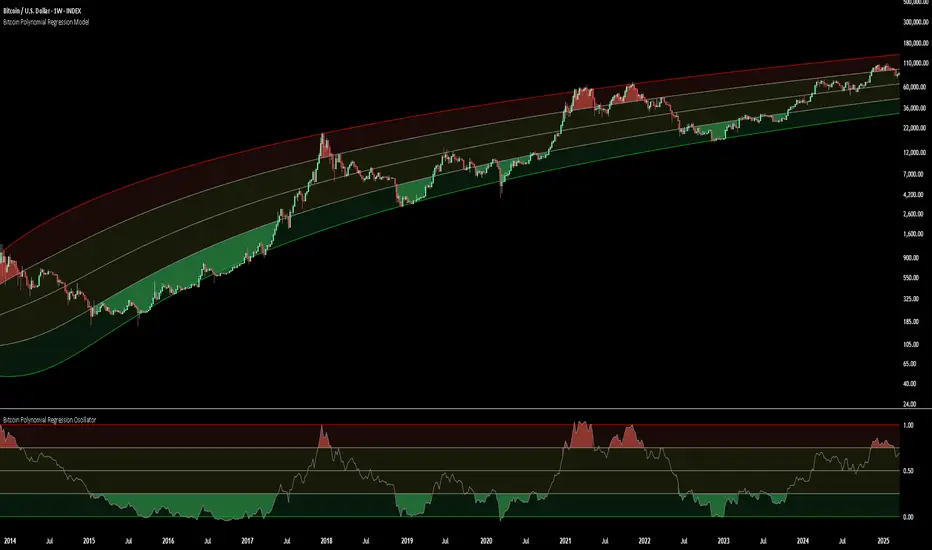
The combination of these two terms is expressed by the graph of the model line (see figure 3), where it can be seen the step from each halving is decaying, and the step up from each halving event is given by a parabolic curve.
NB - The base model has been trained on the first two halving epochs and then seeded (i.e. the first lag point) with the oldest data available.
Constant term: The constant term 0.03 in the equation represents an inherent baseline level of growth in the Bitcoin exchange rate.
In any linear or linear-like model, the constant term, also known as the intercept or bias, represents the value of the dependent variable (in this case, the log-scaled Bitcoin USD exchange rate) when all the independent variables are set to zero.
The constant term indicates that even without considering the effects of the previous day’s exchange rate or halving events, there is a baseline growth in the exchange rate of Bitcoin. This baseline growth could be due to factors such as the network’s overall growth or increasing adoption, or changes in the market structure (more exchanges, changes to the regulatory environment, improved liquidity, more fiat on-ramps etc).
Base Model Regression Diagnostics
Below is a summary of the model generated by the OLS function
OLS Regression Results
\==============================================================================
Dep. Variable: logprice R-squared: 0.999
Model: OLS Adj. R-squared: 0.999
Method: Least Squares F-statistic: 2.041e+06
Date: Fri, 28 Apr 2023 Prob (F-statistic): 0.00
Time: 11:06:58 Log-Likelihood: 3001.6
No. Observations: 2182 AIC: -5997.
Df Residuals: 2179 BIC: -5980.
Df Model: 2
Covariance Type: nonrobust
\==============================================================================
coef std err t P>|t| \
\------------------------------------------------------------------------------
const 0.0292 0.009 3.081 0.002 0.011 0.048
logprice 0.9969 0.001 1012.724 0.000 0.995 0.999
phaseplus -0.0004 0.000 -2.239 0.025 -0.001 -5.3e-05
\==============================================================================
Omnibus: 674.771 Durbin-Watson: 1.901
Prob(Omnibus): 0.000 Jarque-Bera (JB): 24937.353
Skew: -0.765 Prob(JB): 0.00
Kurtosis: 19.491 Cond. No. 255.
\==============================================================================
Below we see some regression diagnostics along with the regression itself.
Diagnostics: We can see that the residuals are looking a little skewed and there is some heteroskedasticity within the residuals. The coefficient of determination, or r2 is very high, but that is to be expected given the momentum term. A better r2 is manually calculated by the sum square of the difference of the model to the untrained data. This can be achieved by the following code:
\# Calculate the out-of-sample R-squared
oos\_mask = df\ >= 2
oos\_actual = df.loc\
oos\_predicted = df.loc\
residuals\_oos = oos\_actual - oos\_predicted
SSR = np.sum(residuals\_oos \*\* 2)
SST = np.sum((oos\_actual - oos\_actual.mean()) \*\* 2)
R2\_oos = 1 - SSR/SST
print("Out-of-sample R-squared:", R2\_oos)
The result is: 0.84, which indicates a very close fit to the out of sample data for the base model, which goes some way to proving our fundamental assumption around subjective value and sound money to be accurate.
Step 2: Adding the Damping Function
Next, we incorporated a damping function to capture the cyclical nature of bull and bear markets. The optimal parameters for the damping function were determined by regressing on the residuals from the base model. The damping function enhances the model’s ability to identify and predict bull and bear cycles in the Bitcoin market. The addition of the damping function to the base model is expressed as the full model equation.
This brings me to the question — why? Why add the damping function to the base model, which is arguably already performing extremely well out of sample and providing valuable insights into the exchange rate movements of Bitcoin.
Fundamental reasoning behind the addition of a damping function:
Subjective Theory of Value: The cyclical component of the damping function, represented by the cosine function, can be thought of as capturing the periodic fluctuations in market sentiment. These fluctuations may arise from various factors, such as changes in investor risk appetite, macroeconomic conditions, or technological advancements. Mathematically, the cyclical component represents the frequency of these fluctuations, while the phase shift (α and β) allows for adjustments in the alignment of these cycles with historical data. This flexibility enables the damping function to account for the heterogeneity in market participants’ preferences and expectations, which is a key aspect of the subjective theory of value.
Time Preference and Market Cycles: The exponential decay component of the damping function, represented by the term e^(-0.0004t), can be linked to the concept of time preference and its impact on market dynamics. In financial markets, the discounting of future cash flows is a common practice, reflecting the time value of money and the inherent uncertainty of future events. The exponential decay in the damping function serves a similar purpose, diminishing the influence of past market cycles as time progresses. This decay term introduces a time-dependent weight to the cyclical component, capturing the dynamic nature of the Bitcoin market and the changing relevance of past events.
Interactions between Cyclical and Exponential Decay Components: The interplay between the cyclical and exponential decay components in the damping function captures the complex dynamics of the Bitcoin market. The damping function effectively models the attenuation of past cycles while also accounting for their periodic nature. This allows the model to adapt to changing market conditions and to provide accurate predictions even in the face of significant volatility or structural shifts.
Now we have the fundamental reasoning for the addition of the function, we can explore the actual implementation and look to other analogies for guidance —
Financial and physical analogies to the damping function:
Mathematical Aspects: The exponential decay component, e^(-0.0004t), attenuates the amplitude of the cyclical component over time. This attenuation factor is crucial in modelling the diminishing influence of past market cycles. The cyclical component, represented by the cosine function, accounts for the periodic nature of market cycles, with α determining the frequency of these cycles and β representing the phase shift. The constant term (+3) ensures that the function remains positive, which is important for practical applications, as the damping function is added to the rest of the model to obtain the final predictions.
Analogies to Existing Damping Functions: The damping function in the BAERM is similar to damped harmonic oscillators found in physics. In a damped harmonic oscillator, an object in motion experiences a restoring force proportional to its displacement from equilibrium and a damping force proportional to its velocity. The equation of motion for a damped harmonic oscillator is:
x’’(t) + 2γx’(t) + ω₀²x(t) = 0
where x(t) is the displacement, ω₀ is the natural frequency, and γ is the damping coefficient. The damping function in the BAERM shares similarities with the solution to this equation, which is typically a product of an exponential decay term and a sinusoidal term. The exponential decay term in the BAERM captures the attenuation of past market cycles, while the cosine term represents the periodic nature of these cycles.
Comparisons with Financial Models: In finance, damped oscillatory models have been applied to model interest rates, stock prices, and exchange rates. The famous Black-Scholes option pricing model, for instance, assumes that stock prices follow a geometric Brownian motion, which can exhibit oscillatory behavior under certain conditions. In fixed income markets, the Cox-Ingersoll-Ross (CIR) model for interest rates also incorporates mean reversion and stochastic volatility, leading to damped oscillatory dynamics.
By drawing on these analogies, we can better understand the technical aspects of the damping function in the BAERM and appreciate its effectiveness in modelling the complex dynamics of the Bitcoin market. The damping function captures both the periodic nature of market cycles and the attenuation of past events’ influence.
Conclusion
In this article, we explored the Bitcoin Auto-correlation Exchange Rate Model (BAERM), a novel 2-step linear regression model for understanding the Bitcoin USD exchange rate. We discussed the model’s components, their interpretations, and the fundamental insights they provide about Bitcoin exchange rate dynamics.
The BAERM’s ability to capture the fundamental properties of Bitcoin is particularly interesting. The framework underlying the model emphasises the importance of individuals’ subjective valuations and preferences in determining prices. The momentum term, which accounts for auto-correlation, is a testament to this idea, as it shows that historical price trends influence market participants’ expectations and valuations. This observation is consistent with the notion that the price of Bitcoin is determined by individuals’ preferences based on past information.
Furthermore, the BAERM incorporates the impact of Bitcoin’s supply dynamics on its price through the halving epoch terms. By acknowledging the significance of supply-side factors, the model reflects the principles of sound money. A limited supply of money, such as that of Bitcoin, maintains its value and purchasing power over time. The halving events, which reduce the block reward, play a crucial role in making Bitcoin increasingly scarce, thus reinforcing its attractiveness as a store of value and a medium of exchange.
The constant term in the model serves as the baseline for the model’s predictions and can be interpreted as an inherent value attributed to Bitcoin. This value emphasizes the significance of the underlying technology, network effects, and Bitcoin’s role as a medium of exchange, store of value, and unit of account. These aspects are all essential for a sound form of money, and the model’s ability to account for them further showcases its strength in capturing the fundamental properties of Bitcoin.
The BAERM offers a potential robust and well-founded methodology for understanding the Bitcoin USD exchange rate, taking into account the key factors that drive it from both supply and demand perspectives.
In conclusion, the Bitcoin Auto-correlation Exchange Rate Model provides a comprehensive fundamentally grounded and hopefully useful framework for understanding the Bitcoin USD exchange rate.
Pine Script® göstergesi