BTC Cap Dominance RSI StrategyThis strategy is based on the BTC Cap Dominance RSI indicator, which is a combination of the RSI of Bitcoin Market Cap and the RSI of Bitcoin Dominance. The concept of this strategy is to get a good grasp of the bitcoin market flow by combining bitcoin dominance as well as bitcoin market cap.
BTC Cap Dominance (BCD) RSI is defined as:
BCD RSI = (BTC Cap RSI + BTC Dominance RSI) / 2
Case 1 (Bull market):
Both Cap RSI and Dominance RSI values are high
Case 2 (Neutral market):
Cap RSI is high but Dominance RSI is low
Cap RSI is low but Dominance RSI is high
Case 3 (Bear market):
Both Cap RSI and Dominance RSI values are low
When the BCD RSI value closes the candle above the Bull level, it triggers a long signal and when the value closes below the Bear level, it triggers a short signal.
(Note) Please note that TradingView's market cap symbols (CRYPTOCAP:TOTAL and CRYPTOCAP:TOTAL2) started in January 2020, so strategy backtesting is possible from this point on.
(Note) Since the real-time BCD RSI value does not come out with this strategy, it is recommended to use it together because the current value can be known and the long-short signal can be predicted in advance by using a separate BCD RSI Index together.
If "Use Combination of dominance RSI ?" is not checked in addition to the recommended default value of the strategy, the recommended values are Length (14), Bull level (74), Bear level (25).
_______________________________________________________________________
이 전략은 비트코인 시가총액의 RSI와 비트코인 도미넌스 RSI를 조합하여 만든 BTC Cap Dominance RSI 지표를 기반으로 만들어졌습니다. 이 전략의 컨셉은 비트코인 시가총액뿐만 아니라 비트코인 도미넌스를 조합함으로써 비트코인 시장 흐름을 잘 파악할 수 있도록 하는 것입니다.
BTC Cap Dominance (BCD) RSI는 다음과 같이 정의하였습니다.
BCD RSI = (BTC Cap RSI + BTC Dominance RSI) / 2
Case 1 (강세 장):
Cap RSI와 Dominance RSI 값 모두 높은 경우
Case 2 (횡보 장):
Cap RSI는 높지만 Dominance RSI는 낮은 경우
Cap RSI는 낮지만 Dominance RSI는 높은 경우
Case 3 (약세 장):
Cap RSI와 Dominance RSI 값 모두 낮은 경우
BCD RSI 값이 Bull level 위에서 캔들 마감할 경우 long 신호를 트리거하고 Bear level 아래에서 캔들 마감할 경우 short 신호를 트리거합니다.
(주의) 트레이딩뷰의 시가총액 심볼들 (CRYPTOCAP:TOTAL과 CRYPTOCAP:TOTAL2)이 2020년 1월부터 시작하였으므로 이 시점부터 전략 백테스팅이 가능한 점을 유의하십시오.
(주의) 이 전략은 실시간 BCD RSI 값이 나오지 않기 때문에 별도의 BCD RSI Index를 함께 사용하면 현재 값을 알 수 있어 롱숏 신호를 사전에 예측할 수 있으므로 함께 사용하기를 권장합니다.
전략의 추천 기본값 외에 "Use Combination of dominance RSI ?"를 체크하지 않는 경우 권장하는 값은 Length (14), Bull level (74), Bear level (25) 입니다.
"2020年3月+中证芯片产业指数+成分股调整" için komut dosyalarını ara

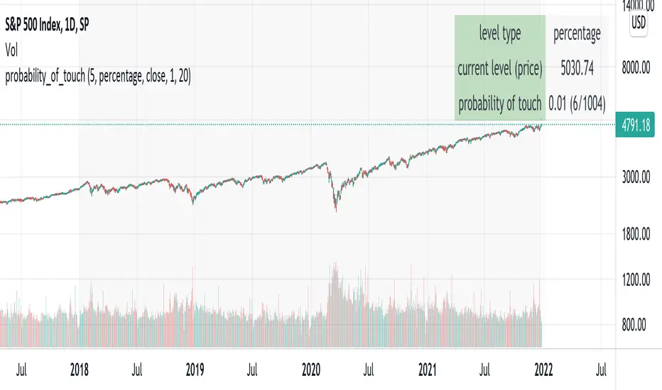
probability_of_touchBased on historical data (rather than theory), calculates the probability of a price level being "touched" within a given time frame. A "touch" means that price exceeded that level at some point. The parameters are:
- level: the "level" to be touched. it can be a number of points, percentage points, or standard deviations away from the mark price. a positive level is above the mark price, and a negative level is below the mark price.
- type: determines the meaning of the "level" parameter. "price" means price points (i.e. the numbers you see on the chart). "percentage" is expressed as a whole number, not a fraction. "stdev" means number of standard deviations, which is computed from recent realized volatlity.
- mark: the point from which the "level" is measured.
- length: the number of days within which the level must be touched.
- window: the number of days used to compute realized volatility. this parameter is only used when "type" is "stdev".
- debug: displays a fuchsia "X" over periods that touched the level. note that only a limited number of labels can be drawn.
- start: only include data after this time in the calculation.
- end: only include data before this time in the calculation.
Example: You want to know how many times Apple stock fell $1 from its closing price the next day, between 2020-02-26 and today. Use the following parameters:
level: -1
type: price
mark: close
length: 1
window:
debug:
start: 2020-02-26
end:
How does the script work? On every bar, the script looks back "length" days and sees if any day exceeded the "mark" price from "length" days ago, plus the limit. The probability is the ratio of such periods wherein price exceeded the limit to the total number of periods.
CDC ActionZone Multi-TF,Mult-Ticker with alert() [P-O-Concept]This is proof-of-concept for using single screen displaying triggering signal of multiple stock/crypto
This source code is subject to the terms of the Mozilla Public License 2.0 at mozilla.org
1. Original CDC Action Zone v3 2020 by © piriya33
Source of original indicator :
2. Table concept/part of code is pulled from Portfolio Tracker
***************************************************************************
CDC Action Zone is based on a simple EMA crossover between EMA12 and EMA26
The zones are defined by the relative position of price in relation to the two EMA lines
Different zones can be use to activate / deactivate other trading strategies
The strategy can also be used on its own with acceptable result, buy on the first green candle
and sell on the first red candle
***************************************************************************
Hint Color Meaning :
Green = FastMA > SlowMA and Price is above FastMA
Blue = FastMA < SlowMA and Price is above both MA
LightBlue = FastMA < SlowMA and Price is between both MA
Red = FastMA < SlowMA and Price is below FastMA
Orange = FastMA > SlowMA and Price is below both MA
Yellow = FastMA > SlowMA and Price is between both MA
Blue/LightBlue/Orange/Yellow should be used with another indicator (such as divergent or so)
Cautions:
- This indicator is not meant to be used as "Signal" or "Trading System"
- This indicator provide a quick-glimpse to multiple ticker in same screen. You'll still have to see indications using original CDC Action Zone (If you're using with CDC System), or combining with another indicator (For shorter tf or scalping, or short/long cover)
- Up to 10 Tickers / Timeframe + Current ticker
Alert Creation Guideline
If this indicator will be used as alert. The timeframe for ticker should be set to "same as" the chart you're using, ie, to set alert on 4h, it should be created in 4h-timeframe (Alert is fired on bar close, using 1D-TABLE in 4H-CHART may trigger alert up to 6 times. else if using in 4H-TABLE in 1D-CHART the alert may not trigger at all)
Considering using ohlc4, hlc3, hl2 for market with no session
PS. Send me a message if you see any bug. (especially if using JSON, I have no chance to test with multiple alert at same tick.)

WEEKLY BTC TRADING SCRYPTWeekly BTC Trading Scrypt(WBTS)
This script is only suggested for cryptocurrencies and weekly buying strategy which is long term.Using it in another markets(e.g forex,stock,e.t.c) is not suggested. The thing makes it different than other strategies we try to understand bull and bear seasons and buying selected crypto currency as using formula if weekly closing value crossover eight weeks simple moving avarage buy,else if selected crypto currency's weekly closing value crossunder eight weeks simple avarage sell. Eight week moving avarage is also uses weekly closing prices but for being able to use this strategy ,trading pair must have more than eight candles in weekly chart otherwise the 8 weeks simple moving avarage value cannot be calculated and script does not work.
This script has a chart called WBTS and it has following features:
Strategy group consist of 3 inputs:
1)Source: Close by default. Our whole strategy uses close values. You can change it but not suggested.
2)Loss Ratio: Because of the cases like the circumstances that manipulates market or high volatility , sometimes graphic show wrong buying signals and this ratio saves user from big money looses(Note : This ratio will always work when selling condition occurs to make user take his profit or prevent him to loss more money because of a wrong positive comes from the indicator.)
3)Reward Ratio : When selling condition happens it will exit user with more profit(if price is already higher than buying point) otherwise it will dimunish loss a bit(if user is below of buying point) or prevents looses(if user is in buying point when selling condition happened.
MA group consist of 2 inputs:
COLOR:Specifies color of the moving avarage.It is equal to #FF3232by hex color code by default.
LINE WIDTH: Specifies linewidth of the moving avarage. It is 2 by default.
GRAPHIC group consist of 2 inputs:
COLOR: It specifies the color of the line which consist of weekly closing prices. It is equal to #6666FF hex color code by default.
LINE WIDTH: Specifies linewidth of the line which consist of weekly closing prices. It is 2 by default.
STRATEGY EXECUTION YEAR: It will show the orders,profits and looses done by script after the input year giving in it.It is 2020 by default.
The last feature is strategy equity,it is not in one of these groups. User should click on settings button on the WBTS indicator than chose Style section and there is a deactivated check box near in the plot section if user activate it, the equity line will show in indicator's graph.
Logic of This Strategy:The story of this strategy began when I studied BTC's price movement from 2020 to today with 8 weeks simple moving avarage (it takes weekly closes as source) and weekly clossing values. I understood that there was a perfect interest between bull and bear market and following conditions:
buy_condition=crossover(weekly_closing_values,8_week_simple_moving_avarage)
sell_condition=crossover(weekly_closing_values,8_week_simple_moving_avarage)
and I tried same thing on the same and bigger time frames("for example i studied how the strategy works from the beginning to today with bitcoin and what is our final equity") with bitcoin and other cryptocurrencies and this made me saw better the relation between giving conditions and general market psychology, however I also witnessed some wrong positives coming by script and used a risk reward ratio to save user and set risk reward ratio 1/3 after a research.
For both conditions(buy_condition and sell_condition),when they are realised,script will alert users and an order will be triggered.
Before finishing the description,from settings/properties/ user can set initial capital,base currency,order size and type,but it is 100000 for initial_amount and 1 contract for order size by default.
In backtesting I used the options like the following example :
Initial capital=1000
Base_curreny=USD
Order size=40 USD
Properties place must set different by every single user according to his or her capital and order size must not be higher than his total money because this script is not the best or a good script for derivatives. It is only written for long term-crypto spot trading and I strongly recommend to users that margin may cause bad results and please do not use it with any margin or any market different than crypto market.
Thank you very much for reading)

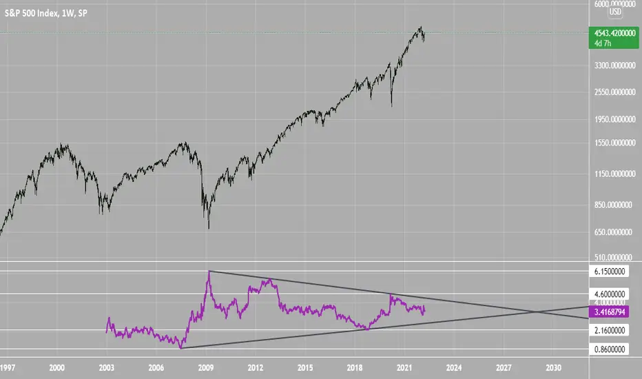
SPX Excess CAPE YieldHere we are looking at the Excess CAPE yield for the SPX500 over the last 100+ years
"A higher CAPE meant a lower subsequent 10-year return, and vice versa. The R-squared was a phenomenally high 0.9 — the CAPE on its own was enough to explain 90% of stocks’ subsequent performance over a decade. The standard deviation was 1.37% — in other words, two-thirds of the time the prediction was within 1.37 percentage points of the eventual outcome: this over a quarter-century that included an equity bubble, a credit bubble, two epic bear markets, and a decade-long bull market."
assets.bwbx.io
In December of 2020 Dr. Robert Shiller the Yale Nobel Laurate suggested that an improvement on CAPE could be made by taking its inverse (the CAPE earnings yield) and subtracting the us10 year treasury yield.
"His model plainly suggests that stocks will do badly over the next 10 years, and that bonds will do even worse. This was the way Shiller put it in a research piece for Barclays Plc in October, (which can be found on SSRN Below):
In summary, investors expect a certain return in equities as compensation for investing in a riskier asset class, and as interest rates have declined, the relative expected return for equities has increased dramatically. We believe this may quantitatively help to explain investors current preference for equities over bonds, and as such the quick recoveries we are observing (with the exception of the UK), whilst still in the midst of a pandemic. In the US in particular, we are once again observing stretched valuations and high CAPE ratios compared to history."
Sources:
papers.ssrn.com
www.bloomberg.com
The standard trading view disclaimer applies to this post -- please consult your own investment advisor before making investment decisions. This post is for observation only and has no warranty etc. www.tradingview.com
Best,
JM
TSI HMA CCIHi!
This strategy has TSI and CCI indicators with the CCI being based on a HMA instead of the Price.
There is a number of conditions that must combine to create buy or sell signals, but it is basically a couple of MA crossovers.
The strategy opens new orders on each candle if the conditions are met, Either direction, so it is hedging.
It wont open new orders if there is a floating loss, and so is constantly attempting to hold a floating profit (drawup instead of drawdown)
But It has a StopLoss (set by user) for closing of losing orders, and it closes all orders in basket style when account is in profit to users set amount target profit.
Low commission set to simulate swap but Forex pairs generally dont have commission like the crypto exchanges do. So if you use this on cryptos, remember to increase the commission to your brokers amount.
Crypto users will likely find that because this opens so many orders the commission could erase its profits.
So i recommend this for Forex only, and perhaps, only NZDUSD 4H chart. other pairs, change settings for.
The strategy has settings for testing on target time spans, so you could test it on just Jan-Feb 2020 for example, if you want, or from Jan 2020 to present day.
Have Fun! Open Script for copy/paste/edit/publish your own version :)

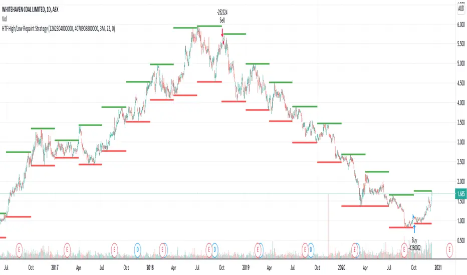
HTF High/Low Repaint StrategyHere is an another attempt to demonstrate repainting and how to avoid them. It happened few times to me that I develop a strategy which is giving immense returns - only to realize after few forward testing that it is repainting. Sometimes, it is well disguised even during forward testing.
In this simple strategy, conditions are as below:
Buy : When a 3M bar produces high and low higher than it's previous 3M bar high, low
Sell : When a 3M bar produces high and low lower than its previous 3M bar high, low.
Default setting is : lookahead = on and offset = 0
This means current 3M bar high low is plotted for all the daily bars within this month. Which means, strategy looks ahead of time to see this 3M bar high is higher than previous 3M bar high during the start of the first daily bar. Hence, this combination leads to massive repaint.
For example, trade made on October 2nd 2018 already knows well ahead of time that price is going to go down in next 3 months:
Similarly, after 2 years on October 2nd 2020 - the strategy already knows that last 3M high is going to be breached on 7th December 2020
Solution: If you are using security for higher timeframes, safer option is always to use offset 1. Further details in the trading view script:
BUT
It may still repaint if we are passing function to security.
For example:
f_secureSecurity(_symbol, _res, _src) => security(_symbol, _res, _src , lookahead = barmerge.lookahead
This function will likely avoid any repainting with Higher timeframe if we are passing in built variables such as high, low, close, open etc. But, if we try to pass supertrend, this will not produce right results. This is because supertrend calculation in turn uses high/low/close values which do not consider the offset while calculating. Hence, even with offset 1, this will still produce issues.
Hence, the call:
= f_secureSecurity(syminfo.tickerid, derivedResolution, supertrend(3,10), offset) will again lead to massive repainting. Solution to this is to implement supertrend function and use high, low, close values derived from secureSecurity.
Quick tips to identify or be suspicious about repainting
Unbelievable results on all timeframes and all instruments with both long and short trades
Lower timeframes giving significantly higher returns on backtest when compared to higher timeframe
If these things happen, be wary about repainting and do a through check of all security function usage in your strategy.
All the best :)
PS: Apply 3-5 days resolution and see the fun. Also, WHC is one hell of a Christmas tree. Could have made immense profit in the same strategy even without repainting.
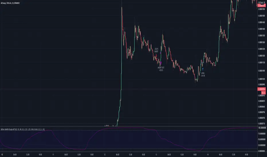
Bitlinc MARSI Study AST w/ Take Profit & Stop loss - beta 0.1This script is beta 0.1 - will update as soon as the script is tradable
This script is based on AST on a 10 minute timeframe. You can change the asset and the timeframe for any asset you want to trade, but for it to work correct ALL settings have to be testes in the Strategy section of the TradingView. Each assets and timeframe require a different mixture of settings. This is NOT a one settings fits all trading for all assets on any timeframe. Below are the settings and explanation on how it works.
How it fires a buy / sell:
The script will plot an RSI with upper and lower bands in a separate indicator window. The idea behind this script is to fire a LONG when MA crosses OVER lower band and fire a SHORT when the MA crosses under the lower band. Each order that fires is an OCO (Order Cancels Order) for pyramiding.
Settings:
You have full control of these settings as mentioned above, you must configure every part of this script for each asset and timeframe you trade.
- Length of MA
- Length
- Upper bands of RSI
- Lower bands of RSI
- Take profit percentage
- Stop loss percentage
- Month to start and end the strategy (within 2020)
- Day to start and end the strategy (within 2020)
- Quantity type
- Slippage
- Pyramiding
***Remember that after the signal to enter or exit a trade is fired, the alert will trigger AFTER the close of the candle that caused the tigger to fire
Haemil-ri Moving Average Line/Created by user dunsan2000 updated 2020/8/20
//It is a moving average that is easy to use in Haemil-ri.
//둔산2000 만듬, 2020/8/20 수정됨
//해밀리에서 사용하기에 편한 이동평균선 입니다.

LB Squeeze Momentum DivergencesThis study tries to highlight LazyBear Squeeze Momentum divergences
as they are defined by
TradingLatino TradingView user
Squeeze momentum green peaks are connected by a line
Associated prices to these green peaks are also connected
If both lines have a different slope orientation
then there is a divergence.
It only shows two last divergence lines and angles.
The original chart screenshot shows some divergence lines
on the top or main chart
these were drawn manually
because you cannot write to two different charts
from the same pine script study (Well, not in August 2020 anyways)
It's aimed at BTCUSDT pair and 4h timeframe.
HOW IT WORKS
Simple geometric mathematics are used
to calculate the two lines degrees
Then both degrees are compared
to show if both lines agree ( // or \\ )
or if they disagree ( /\ or \/ )
SETTINGS
(SQZDiver) Show degrees : Show degrees of each Squeeze Momentum Divergence
lines to the x-axis.
(SQZDiver) Show desviation labels : Whether to show
or not desviation labels for the Squeeze Momentum Divergences.
(SQZDiver) Show desviation lines : Whether to show
or not desviation lines for the Squeeze Momentum Divergences.
(ADX) Smoothing
(ADX) DI Length
(ADX) key level
(ADX) Print : Whether to show
or not scaled ADX line
(SQZMOM) BB Length
(SQZMOM) BB MultFactor
(SQZMOM) KC Length
(SQZMOM) KC MultFactor
(SQZMOM) Use TrueRange (KC)
(SQZMOM) Print : Whether to show
or not Squeeze Momentum indicator.
WARNING
Some securities and timeframes might output degrees
too next to zero.
The code might need to be tweaked to meet your needs.
USAGE
One strategy is to sell when you are in a long entry
when you find out that the price slope is upwards ( / )
while the lb smilb slope is downwards: ( \ )
E.g. You will see:
/
\
on the indicator.
Why?
Because it might signal you that the price is
going to correct downwards soon.
FEEDBACK 1
Please let me know if there is any
other strategy based on the red side of
LB Squeeze Momentum
so that I might add support for it in the future.
FEEDBACK 2
Calculating degrees in a chart
with a different x-axis scale
is a nightmare
that's why I did not a range settings
so that values next to zero are
converted into zero
and thus showing an horizontal line.
Feedback is welcome on this matter.
EXTRA 1
If you turn off showing the divergence lines
and if you turn off showing the divergence labels
you almost get what TradingLatino user uses
as its default momentum indicator.
EXTRA 2
Optionally this indicator can show you
a rescaled ADX (it only works properly on 2020 Bitcoin charts)
ABOUT COLOURS
TradingLatino user has both dark green and light green
inverted compared to this LB SQZMOM chart.
CREDITS
I have reused and adapted some code from
'Squeeze Momentum Indicator' study
which it's from TradingView LazyBear user.
I have reused and adapted some code from
'Directional Movement Index + ADX & Keylevel Support' study
which it's from TradingView console user.

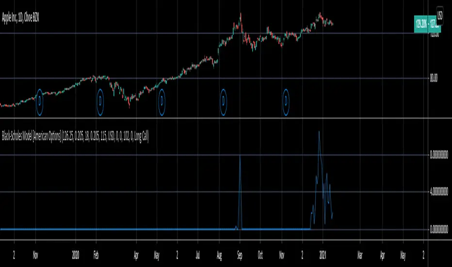
Black-Scholes Model for American OptionsThis model uses Black's Approximation to price American Options. Black's Approximation is an extension of the traditional Black-Scholes model that allows the price of American Options to be approximated within the Black-Scholes Framework. This is necessary because the traditional Black-Scholes model only works on options that are exercised at expiry, not before; like American Options can be.
Black's Approximation approximates the value of an American option by:
1st. Calculating the theoretical price of a european call or put based on the strike price (K), spot price (S), annual return (sigma), time until expiry (T), times until the next 2 ex-dividend dates (t1 & t2), and the dividend paid out at times t1 and t2 (D1 and D2).
2nd. The theoretical price of an option expiring on the second ex-dividend date (t2) is calculated. This replicates exercising the option early.
3rd. Finally, the highest price of the two theoretical prices calculated in steps 1 & 2 is chosen as the approximated price.
How to use this:
1st. Input your strike price.
2nd. Input the risk-free-rate of the currency the option is based in.
3rd. Input the dividend yield for the next ex-dividend date. For example AAPL's dividend yield is 0.82 and will be paid out on August 7,2020.
4th. Input the time until the next ex-dividend date. For example AAPL's next ex-dividend date is August 7,2020, which is 61 days away. So you'd input 61 (this includes weekends and holidays).
5th. Input the dividend yield for the ex-dividend date after the next one. For example AAPL's dividend yield after the next one is 0.82 and will be paid out on November 6, 2020.
6th. Input the time until the next furthest ex-dividend date. For example AAPL's next ex-dividend date after Aug 7th, is on November 6, 2020, which is 152 days away. So you'd input 152 (this includes weekends and holidays).
7th. Input your time until expiry. You can do so in terms of days, hours, and minutes.
8th. Input your chart time-frame in term of minutes. For example, if you're using the 1 min time-frame enter 1, 4hr time-frame enter 480, daily time-frame enter 1440.
9th. Lastly, pick what type of option you want data for: Long Call or Long Put.
*Disclaimer, because Black's Approximation is mostly geared towards stocks, this will only work for stocks. Also, the time variables: time until expiry and time until the ex-dividend dates; don't automatically update. So you will have to update them each day.
Weis Pip Wave jayyWhat you see here is the Weis pip wave. The Weis pip wave shows how far in price a Weis wave has traveled through the duration of a Weis wave. The Weis pip wave is used in combination with the Weis cumulative volume wave. The two waves must be set to the same "wave size" and using the same method as described by Weis.
Using the traditional Weis method simply enter the desired wave size in the box "Select Weis Wave Size". In the example shown, it is set to 5 points. Each wave for each security and each timeframe requires its own wave size. Although not the traditional method a more automatic way to set wave size would be to use ATR. This is not the true Weis method but it does give you similar waves and, importantly, without the hassle of selecting a wave size for every chart. Once the Weis wave size is set then the pip wave will be shown.
I have put a zigzag of a 5 point Weis wave on the above bar chart. I have added it to allow your eye to get a better appreciation for Weis wave pivot points. You will notice that the wave is not in straight lines connecting wave tops to bottoms this is a function of the limitations of Pinescript version 1. This script would need to be in version 4 to allow straight lines. I will elaborate on the Weis pip zigzag script.
What is a Weis wave? David Weis has been recognized as a Wyckoff method analyst he has written two books one of which, Trades About to Happen, describes the evolution of the now popular Weis wave. The method employed by Weis is to identify waves of price action and to compare the strength of the waves on characteristics of wave strength. Chief among the characteristics of strength is the cumulative volume of the wave. There are other markers that Weis uses as well for example how the actual price difference between the start of the Weis wave from start to finish. Weis also uses time, particularly when using a Renko chart. Weis specifically uses candle/bar closes to define all wave action.
David Weis did a futures.io video which is a popular source of information about his method.
Cheers jayy
PS This script was published a day ago, however, I had included some links to the website of a person that uses Weis pip waves and also a dropbox link that contains the Weis wave chart for May 27, 2020, published by David Weis. Providing those links is against TV policy and so the script was hidden by TV. This is the identical script with the identical settings but without the offending links. If you want to see the pip Weis method in practice then search Weis pip wave. I have absolutely no affiliation. If you want to see Weis chart in pdf then message me and I will give a link or the Weis pdf. Why would you want to see the Weis chart for May 27, 2020? Merely to confirm the veracity of my algorithm. You could compare my chart () from the same period to the Weis chart. Both waves are for the ES!1 4 hour chart and both for a wave size of 5.

ApopheniaPays Crossing detector & 2-field date/time entryYou specify a horizontal line by value, start date/time, and end date/time, and choose a data source (bar close is the default) and it will label count how many times that source crosses that line between those dates/times.
Enter the start and end dates for your horizontal line as MMDDYY and HHMM (24 hour time).
: Jan 17, 2020 would be 11720 (properly it would be 011720, but Pine inputs delete leading 0s).
: November 17, 2020 would be 110720.
: 8:30 AM would be 0830.
: 8:30 PM would be 2030.
Remember to enter the right time zone.
I believe nobody else has published a 2-input date/time picker on TV, at least the last time I checked they hadn't, they all make you input M,D,Y,H,M as separate fields. Ugh!
If you use any parts of this code, please credit me. If somehow you happen to make a lot of money using this code, please think about what a fair share would be to pay me for my help, then give that amount to a worthwhile charity.

.BXBT IndexThe current .BXBT index weighted as close as possible to BitMEX's with updates as BitMEX refreshes their index.
Difference between this and the script titled '2020 March 27 .BXBT Index': this one will receive updates because it doesn't have a date in its title.
Methodology
www.bitmex.com
"BitMEX Index Weights, assuming no constituent exchanges have been excluded due to Index Protection Rules, last updated 27 December 2019 at 12:00:05 UTC."
Binance: -
Bitstamp: 10.61%
Bittrex: 2.53%
Coinbase: 52.30%
Gemini: 6.89%
Huobi: -
Itbit: 4.21%
Kraken: 23.46%
Poloniex: -
ItBit's weight is combined with Gemini's due to ItBit not being on TradingView as of now. BITTREX:BTCUSD substituted with BITTREX:BTCUSDT*POLONIEX:USDTUSD to backfill because Bittrex only recently (late 2018) started to offer a fiat BTC/USD pair. Not that it matters since the index used in 2018 didn't include Bittrex if I remember correctly.
What is actually used for 27/12/2019 to 27/03/2020:
Binance: -
Bitstamp: 10.61%
Bittrex: 2.53%
Coinbase: 52.30%
Gemini: 11.10%
Huobi: -
Itbit: -
Kraken: 23.46%
Poloniex: -
Options:
Toggle candlesticks or close line
Change price source to be used for indicators
To be added: Change quarter to show indexes for different times, with labels that apply to the appropriate index used
Reasons to use this vs. the index itself: (not many)
It is helpful as a reference for other indicators or creation of an index.

Stochastic Pop and Drop by Jake Bernstein v1 [Bitduke]I found a simple strategy by Jake Bernstein, modified it a little and created a strategy with Risk Management System (SL+TP); After that I test it on the different cryptocurrency pairs.
About the Indicator
Basically it's the strategy of 2 indicators: Stochastic Oscillator to define the bias and Average Directional Index to confirm it.
One again, It uses Stochastic Oscillator to define the trading bias. In particular, the trading bias was deemed bullish when the weekly 14-period Stochastic Oscillator was above some default value (in him paper - 50) and rising and vice versa.
Once the trading bias is established, Steckler used the Average Directional Index (ADX) to define a slowdown in the trend. ADX measures the strength of the trend and a move below 20 signals a weak trend.
Modifications
I didn't implement Average Directional Index (ADX) and test just different sources for data, oscillator periods and different levels in relation to the crypto market.
So, it shows good results with two tight thresholds at 55 and 45 level.
The bar chart below the defining the bullish and bearish periods (green and red) and gives a signal to enter the trade (purple bars).
Backtesting
Backtested on XBTUSD , BTCPERP (FTX) pairs. You may notice it shows good results on 3h timeframe.
Relatively low drawdown
~ 10% (from 2019 to date) FTX
~ 22% (4 years from 2016) Bitmex
I backtested on the different altcoin pairs as well, but the results were just not good.
Relatively good results were shown by some index pairs from the FTX exchange ( FTX:SHITPERP ), but I think there is a few data for backtesting to be asure in them.
Bitmex 3h (2017 - 2020) :
i.imgur.com
FTX 3h (2019 - 2020):
i.imgur.com
Possible Improvements
- Regarding trading algorithm it would be good to check with strategy with ADX somehow. Maybe for the better entries
- As for Risk Management system, it can be improved by adding trailing stop to the strategy.
Link: school.stockcharts.com

Double MA CCI"What is the Commodity Channel Index (CCI)?
Developed by Donald Lambert, the Commodity Channel Index (CCI) is a momentum-based oscillator used to help determine when an investment vehicle is reaching a condition of being overbought or oversold. It is also used to assess price trend direction and strength. This information allows traders to determine if they want to enter or exit a trade, refrain from taking a trade, or add to an existing position. In this way, the indicator can be used to provide trade signals when it acts in a certain way.
KEY TAKEAWAYS
• The CCI measures the difference between the current price and the historical average price.
• When the CCI is above zero it indicates the price is above the historic average. When CCI is below zero, the price is below the hsitoric average.
• High readings of 100 or above, for example, indicate the price is well above the historic average and the trend has been strong to the upside.
• Low readings below -100, for example, indicate the price is well below the historic average and the trend has been strong to the downside.
• Going from negative or near-zero readings to +100 can be used as a signal to watch for an emerging uptrend.
• Going from positive or near-zero readings to -100 may indicate an emerging downtrend.
• CCI is an unbounded indicator meaning it can go higher or lower indefinitely. For this reason, overbought and oversold levels are typically determined for each individual asset by looking at historical extreme CCI levels where the price reversed from." ----> 1
SOURCE
1: (SINCE IM NOT A "PRO" MEMBER I C'ANT POST THE SOUCRE URL..., webpage consulted at : 8:50 GMT -5 ; the 2020-01-18)
I- Added a 2nd MA length and changed the default values of the source type and switched the SMA to a MA.
II- In process to add analytic MACD histogram correlation and if possible, ploting a relative histogram between the CCI upper and lower band.
P.S.:
Don't set your moving averages lengths to far from each other... This could result in fewer convergence and divergence, also in fewer crossing MA's.
Have a good year 2020 !!
//----CODER----//
R.V.

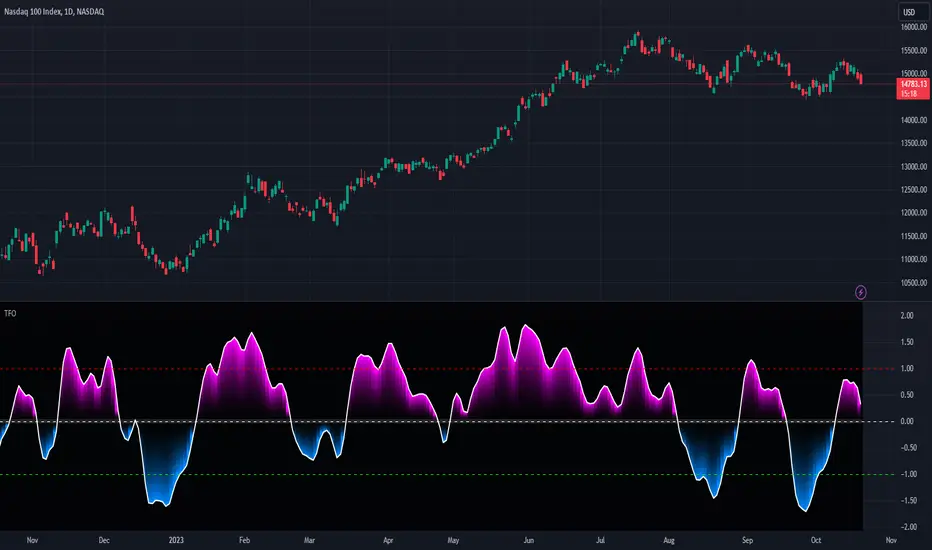
Reflex Oscillator - Dr. John EhlersHot off the press, I present this NEW "Reflex Oscillator" employing PSv4.0, originally formulated by Dr. John Ehlers for TASC - February 2020 Traders Tips. John Ehlers might describe it's novel characteristics as being a reversal sensitive near zero-lag averaging indicator retaining the CYCLE component. Also, I would add that irregardless of the sampling interval, this indicator has a bound range between +/-2.0 on "1 second" candles all the way up to "1 month" candle durations. This indicator also has a companion indicator entitled "TrendFlex Oscillator". I have published it in tandem with this one in my scripts profile.
One notable difference between this and the original formulation is that I have added an independent control for the Super Smoother. This "tweak" is enabled by applying the override and adjusting it's period. There is a "Post Smooth" input() that "tweaks" the internal Reflex EMA too. Keep in mind that my intention of adding tweaks is solely for experimentation with the original formulation.
I also added adjustable levels for those of you that may wish to employ alertcondition()s to this indicator somehow. Providing a more utilitarian approach, I created this with an easy to use reusable function named reflex(). As always, I have included advanced Pine programming techniques that conform to proper "Pine Etiquette". Being this is one of John Ehlers' first two simultaneously released indicators for 2020, I felt a few more bells and whistles were appropriate as a proper contribution to the Tradingview community.
Features List Includes:
Dark Background - Easily disabled in indicator Settings->Style for "Light" charts or with Pine commenting
AND much, much more... You have the source!
The comments section below is solely just for commenting and other remarks, ideas, compliments, etc... regarding only this indicator, not others. When available time provides itself, I will consider your inquiries, thoughts, and concepts presented below in the comments section, should you have any questions or comments regarding this indicator. When my indicators achieve more prevalent use by TV members, I may implement more ideas when they present themselves as worthy additions. As always, "Like" it if you simply just like it with a proper thumbs up, and also return to my scripts list occasionally for additional postings. Have a profitable future everyone!

TrendFlex Oscillator - Dr. John EhlersHot off the press, I present this NEW "TrendFlex Oscillator" employing PSv4.0, originally formulated by Dr. John Ehlers for TASC - February 2020 Traders Tips. John Ehlers might describe it's novel characteristics as being a reversal sensitive near zero-lag averaging indicator retaining the TREND component. Also, I would add that irregardless of the sampling interval, this indicator has a bound range between +/-2.0 on "1 second" candles all the way up to "1 month" candle durations. This indicator also has a companion indicator entitled "Reflex Oscillator". I have published it in tandem with this one in my scripts profile.
One notable difference between this and the original formulation is that I have added an independent control for the Super Smoother. This "tweak" is enabled by applying the override and adjusting it's period. There is a "Post Smooth" input() that "tweaks" the internal TrendFlex EMA too. Keep in mind that my intention of adding tweaks is solely for experimentation with the original formulation.
I also added adjustable levels for those of you that may wish to employ alertcondition()s to this indicator somehow. Providing a more utilitarian approach, I created this with an easy to use reusable function named trendflex(). As always, I have included advanced Pine programming techniques that conform to proper "Pine Ettiquette". Being this is one of John Ehlers' first two simultaneously released indicators for 2020, I felt a few more bells and whistles were appropriate as a proper contribution to the Tradingview community.
Features List Includes:
Dark Background - Easily disabled in indicator Settings->Style for "Light" charts or with Pine commenting
AND much, much more... You have the source!
The comments section below is solely just for commenting and other remarks, ideas, compliments, etc... regarding only this indicator, not others. When available time provides itself, I will consider your inquiries, thoughts, and concepts presented below in the comments section, should you have any questions or comments regarding this indicator. When my indicators achieve more prevalent use by TV members, I may implement more ideas when they present themselves as worthy additions. As always, "Like" it if you simply just like it with a proper thumbs up, and also return to my scripts list occasionally for additional postings. Have a profitable future everyone!
Ichimoku Kinkō hyō Keizen 改善
The script is not finnished yet and show's an other interpretation of how it could be scripted
Step -1 is complete... Basic Ichimoku with asjutable length and editable lines colors and visibilities.
Step -2 in progress... Adding ability to une multiple Spans, sens and Kumo on higher and lower timeframe.
Your Step : Like and Share ;) have a good year 2020 !
2020-01-06 /--------/ -R.V.
Trend Speed Analyzer + alerts//@version=6
indicator('Trend Speed Analyzer + alerts', overlay = false)
//~~}
// ~~ Tooltips {
string t1 = 'Maximum Length: This parameter sets the upper limit for the number of bars considered in the dynamic moving average. A higher value smooths out the trend line, making it less reactive to minor fluctuations but slower to adapt to sudden price movements. Use higher values for long-term trend analysis and lower values for faster-moving markets.'
string t2 = 'Accelerator Multiplier: Adjusts the responsiveness of the dynamic moving average to price changes. A larger value makes the trend more reactive but can introduce noise in choppy markets. Lower values create a smoother trend but may lag behind rapid price movements. This is particularly useful in volatile markets where precise sensitivity is needed.'
string t5 = 'Enable Candles: When enabled, the candlesticks on the chart will be color-coded based on the calculated trend speed. This provides a visual representation of momentum, making it easier to spot shifts in market dynamics. Disable this if you prefer the standard candlestick colors.'
string t6 = 'Collection Period: Defines the number of bars used to normalize trend speed values. A higher value includes a broader historical range, smoothing out the speed calculation. Lower values make the speed analysis more sensitive to recent price changes, ideal for short-term trading.'
string t7 = 'Enable Table: Activates a statistical table that provides an overview of key metrics, such as average wave height, maximum wave height, dominance, and wave ratios. Useful for traders who want numerical insights to complement visual trend analysis.'
string t8 = 'Lookback Period: Determines how many historical bars are used for calculating bullish and bearish wave data. A longer lookback period provides a more comprehensive view of market trends but may dilute sensitivity to recent market conditions. Shorter periods focus on recent data.'
string t9 = 'Start Date: Sets the starting point for all calculations. This allows you to analyze data only from a specific date onward, which is useful for isolating trends within a certain period or avoiding historical noise.'
string t10 = 'Timer Option: Select between using a custom start date or starting from the first available bar on the chart. The \'Custom\' option works with the Start Date setting, while \'From start\' includes all available data.'
// Tooltips for Table Cells
string tt1 = 'Average Wave: Shows the average size of bullish or bearish waves during the lookback period. Use this to assess overall market strength. Larger values indicate stronger trends, and comparing bullish vs bearish averages can reveal market bias. For instance, a higher bullish average suggests a stronger uptrend.'
string tt2 = 'Max Wave: Displays the largest bullish or bearish wave during the lookback period. Use this to identify peak market momentum. A significantly higher bullish or bearish max wave indicates where the market may have shown extreme trend strength in that direction.'
string tt3 = 'Current Wave Ratio (Average): Compares the current wave\'s size to the average wave size for both bullish and bearish trends. A value above 1 indicates the current wave is stronger than the historical average, which may signal increased market momentum. Use this to evaluate if the current move is significant compared to past trends.'
string tt4 = 'Current Wave Ratio (Max): Compares the current wave\'s size to the maximum wave size for both bullish and bearish trends. A value above 1 suggests the current wave is setting new highs in strength, which could indicate a breakout or strong momentum in the trend direction.'
string tt5 = 'Dominance (Average): The net difference between the average bullish and bearish wave sizes. Positive values suggest bullish dominance over time, while negative values indicate bearish dominance. Use this to determine which side (bulls or bears) has had consistent control of the market over the lookback period.'
string tt6 = 'Dominance (Max): The net difference between the largest bullish and bearish wave sizes. Positive values suggest bulls have dominated with stronger individual waves, while negative values indicate bears have produced stronger waves. Use this to gauge the most significant power shifts in the market.'
//~~~~~~~~~~~~~~~~~~~~~~~~~~~~~~~~~~~~~~~~~~~~~~~~~~~~~~~~~~~~~~~~~~~~~~~~~~~~~~~~~~~~~~~~~~~~~~~~~~~~~~~~~~~~~~~~~~~~~}
max_length = input.int(50, minval = 1, title = 'Maximum Length', group = 'Dynamic Moving Average', tooltip = t1)
accel_multiplier = input.float(5.0, minval = 0.0, step = 1.1, title = 'Accelerator Multiplier', group = 'Dynamic Moving Average', tooltip = t2)
tbl_ = input.bool(true, title = 'Enable Table', group = 'Wave Analysis', tooltip = t7)
lookback_period = input.int(100, minval = 1, step = 1, title = 'Lookback Period', group = 'Wave Analysis', tooltip = t8)
candle = input.bool(true, title = 'Enable Candles', group = 'Trend Visualization', tooltip = t5)
collen = input.int(100, step = 10, minval = 5, title = 'Collection Period', group = 'Trend Visualization', tooltip = t6)
up_col = input.color(color.lime, title = 'Dynamic Trend', group = 'Trend Visualization', inline = 'Trend')
dn_col = input.color(color.red, title = '', group = 'Trend Visualization', inline = 'Trend')
up_hist_col = input.color(#82ffc3, title = 'Trend Speed Up', group = 'Trend Visualization', inline = 'up')
up_hist_col_ = input.color(color.lime, title = '', group = 'Trend Visualization', inline = 'up')
dn_hist_col = input.color(color.red, title = 'Trend Speed Dn', group = 'Trend Visualization', inline = 'dn')
dn_hist_col_ = input.color(#f78c8c, title = '', group = 'Trend Visualization', inline = 'dn')
start = input.time(timestamp('1 Jan 2020 00:00 +0000'), title = 'Start Date', group = 'Time Settings', tooltip = t9, inline = 'startdate')
timer = input.string('From start', title = 'Timer Option', options = , group = 'Time Settings', tooltip = t10, inline = 'startdate')
// ~~ Dynamic Average {
counts_diff = close
max_abs_counts_diff = ta.highest(math.abs(counts_diff), 200)
counts_diff_norm = (counts_diff + max_abs_counts_diff) / (2 * max_abs_counts_diff)
dyn_length = 5 + counts_diff_norm * (max_length - 5)
// ~~ Function to compute the accelerator factor with normalization of delta_counts_diff {
calc_accel_factor(float counts_diff, float prev_counts_diff) =>
delta_counts_diff = math.abs(counts_diff - prev_counts_diff)
float max_delta_counts_diff = ta.highest(delta_counts_diff, 200)
max_delta_counts_diff := max_delta_counts_diff == 0 ? 1 : max_delta_counts_diff
float accel_factor = delta_counts_diff / max_delta_counts_diff
accel_factor
//~~~~~~~~~~~~~~~~~~~~~~~~~~~~~~~~~~~~~~~~~~~~~~~~~~~~~~~~~~~~~~~~~~~~~~~~~~~~~~~~~~~~~~~~~~~~~~~~~~~~~~~~~~~~~~~~~~~~~}
// ~~ Function to adjust alpha using the accelerator factor {
adjust_alpha(float dyn_length, float accel_factor, float accel_multiplier) =>
alpha_base = 2 / (dyn_length + 1)
alpha = alpha_base * (1 + accel_factor * accel_multiplier)
alpha := math.min(1, alpha)
alpha
//~~~~~~~~~~~~~~~~~~~~~~~~~~~~~~~~~~~~~~~~~~~~~~~~~~~~~~~~~~~~~~~~~~~~~~~~~~~~~~~~~~~~~~~~~~~~~~~~~~~~~~~~~~~~~~~~~~~~~}
// ~~ Accelerator Factor
accel_factor = calc_accel_factor(counts_diff, nz(counts_diff ))
alpha = adjust_alpha(dyn_length, accel_factor, accel_multiplier)
// ~~ Compute dynamic Ema
var float dyn_ema = na
dyn_ema := na(dyn_ema ) ? close : alpha * close + (1 - alpha) * dyn_ema
//~~~~~~~~~~~~~~~~~~~~~~~~~~~~~~~~~~~~~~~~~~~~~~~~~~~~~~~~~~~~~~~~~~~~~~~~~~~~~~~~~~~~~~~~~~~~~~~~~~~~~~~~~~~~~~~~~~~~~}
// ~~ Trend Speed {
trend = dyn_ema
bullsrc = close
bearsrc = close
type TrendData
array change
array t
StartTime() =>
time > start
var bullish = TrendData.new(array.new(), array.new())
var bearish = TrendData.new(array.new(), array.new())
var x1 = int(na)
var y1 = float(na)
var pos = 0
var speed = 0.0
c = ta.rma(close, 10)
o = ta.rma(open, 10)
// ~~ First value {
if na(x1) and StartTime() or na(x1) and timer == 'From start'
x1 := bar_index
y1 := o
y1
//~~~~~~~~~~~~~~~~~~~~~~~~~~~~~~~~~~~~~~~~~~~~~~~~~~~~~~~~~~~~~~~~~~~~~~~~~~~~~~~~~~~~~~~~~~~~~~~~~~~~~~~~~~~~~~~~~~~~~}
// ~~ Trend direction {
if StartTime() or timer == 'From start'
if bullsrc > trend and bullsrc <= trend
bearish.change.unshift(ta.lowest(speed, bar_index - x1))
bearish.t.unshift(bar_index - x1)
x1 := bar_index
y1 := bullsrc
pos := 1
speed := c - o
speed
if bearsrc < trend and bearsrc >= trend
bullish.change.unshift(ta.highest(speed, bar_index - x1))
bullish.t.unshift(bar_index - x1)
x1 := bar_index
y1 := bearsrc
pos := -1
speed := c - o
speed
speed := speed + c - o
speedGradient = color.from_gradient(speed, ta.min(-speed / 3), ta.max(speed / 3), color.red, color.lime)
trendspeed = ta.hma(speed, 5)
//~~~~~~~~~~~~~~~~~~~~~~~~~~~~~~~~~~~~~~~~~~~~~~~~~~~~~~~~~~~~~~~~~~~~~~~~~~~~~~~~~~~~~~~~~~~~~~~~~~~~~~~~~~~~~~~~~~~~~}
//~~~~~~~~~~~~~~~~~~~~~~~~~~~~~~~~~~~~~~~~~~~~~~~~~~~~~~~~~~~~~~~~~~~~~~~~~~~~~~~~~~~~~~~~~~~~~~~~~~~~~~~~~~~~~~~~~~~~~}
// ~~ Plots {
rma_dyn_ema(x, p) =>
average = ta.rma(dyn_ema , p)
average
colour = ta.wma(close, 2) > dyn_ema ? up_col : dn_col
fillColor = rma_dyn_ema(0, 5) > rma_dyn_ema(1, 5) ? color.new(up_col, 70) : color.new(dn_col, 70)
p1 = plot(dyn_ema, color = colour, linewidth = 2, title = 'Dynamic Trend', force_overlay = true)
p2 = plot(ta.rma(hl2, 50), display = display.none, editable = false, force_overlay = true)
//~~~~~~~~~~~~~~~~~~~~~~~~~~~~~~~~~~~~~~~~~~~~~~~~~~~~~~~~~~~~~~~~~~~~~~~~~~~~~~~~~~~~~~~~~~~~~~~~~~~~~~~~~~~~~~~~~~~~~}
min_speed = ta.lowest(speed, collen)
max_speed = ta.highest(speed, collen)
normalized_speed = (speed - min_speed) / (max_speed - min_speed)
speedGradient1 = speed < 0 ? color.from_gradient(normalized_speed, 0.0, 0.5, dn_hist_col, dn_hist_col_) : color.from_gradient(normalized_speed, 0.5, 1.0, up_hist_col, up_hist_col_)
plot(StartTime() or timer == 'From start' ? trendspeed : na, title = 'Trend Speed', color = speedGradient1, style = plot.style_columns)
plotcandle(open, high, low, close, color = candle ? speedGradient1 : na, wickcolor = candle ? speedGradient1 : na, bordercolor = candle ? speedGradient1 : na, force_overlay = true)
//~~~~~~~~~~~~~~~~~~~~~~~~~~~~~~~~~~~~~~~~~~~~~~~~~~~~~~~~~~~~~~~~~~~~~~~~~~~~~~~~~~~~~~~~~~~~~~~~~~~~~~~~~~~~~~~~~~~~~}
// ~~ Table {
if barstate.islast and tbl_
bullish_recent = bullish.change.slice(0, math.min(lookback_period, bullish.change.size()))
bearish_recent = bearish.change.slice(0, math.min(lookback_period, bearish.change.size()))
bull_max = bullish_recent.max()
bear_max = bearish_recent.min()
bull_avg = bullish_recent.avg()
bear_avg = bearish_recent.avg()
wave_size_ratio_avg = bull_avg / math.abs(bear_avg)
wave_size_text_avg = str.tostring(math.round(wave_size_ratio_avg, 2)) + 'x'
wave_size_color_avg = wave_size_ratio_avg > 0 ? color.lime : color.red
wave_size_ratio_max = bull_max / math.abs(bear_max)
wave_size_text_max = str.tostring(math.round(wave_size_ratio_max, 2)) + 'x'
wave_size_color_max = wave_size_ratio_max > 0 ? color.lime : color.red
dominance_avg_value = bull_avg - math.abs(bear_avg)
dominance_avg_text = dominance_avg_value > 0 ? 'Bullish +' + str.tostring(math.round(wave_size_ratio_avg, 2)) + 'x' : 'Bearish -' + str.tostring(math.round(1 / wave_size_ratio_avg, 2)) + 'x'
dominance_avg_color = dominance_avg_value > 0 ? color.lime : color.red
dominance_max_value = bull_max - math.abs(bear_max)
dominance_max_text = dominance_max_value > 0 ? 'Bullish +' + str.tostring(math.round(wave_size_ratio_max, 2)) + 'x' : 'Bearish -' + str.tostring(math.round(1 / wave_size_ratio_max, 2)) + 'x'
dominance_max_color = dominance_max_value > 0 ? color.lime : color.red
current_wave = speed
current_wave_color = current_wave > 0 ? color.lime : color.red
current_ratio_avg = current_wave > 0 ? current_wave / bull_avg : current_wave / math.abs(bear_avg)
current_ratio_max = current_wave > 0 ? current_wave / bull_max : current_wave / math.abs(bear_max)
current_text_avg = str.tostring(math.round(current_ratio_avg, 2)) + 'x'
current_text_max = str.tostring(math.round(current_ratio_max, 2)) + 'x'
current_color_avg = current_ratio_avg > 0 ? color.lime : color.red
current_color_max = current_ratio_max > 0 ? color.lime : color.red
var tbl = table.new(position.top_right, 3, 3, force_overlay = true)
table.cell(tbl, 0, 0, '', text_color = chart.fg_color, tooltip = '')
table.cell(tbl, 0, 1, 'Average Wave', text_color = chart.fg_color, tooltip = tt1)
table.cell(tbl, 0, 2, 'Max Wave', text_color = chart.fg_color, tooltip = tt2)
table.cell(tbl, 1, 0, 'Current Wave Ratio', text_color = chart.fg_color, tooltip = '')
table.cell(tbl, 1, 1, current_text_avg, text_color = current_color_avg, tooltip = tt3)
table.cell(tbl, 1, 2, current_text_max, text_color = current_color_max, tooltip = tt4)
table.cell(tbl, 2, 0, 'Dominance', text_color = chart.fg_color, tooltip = '')
table.cell(tbl, 2, 1, dominance_avg_text, text_color = dominance_avg_color, tooltip = tt5)
table.cell(tbl, 2, 2, dominance_max_text, text_color = dominance_max_color, tooltip = tt6)
// ─────────────────────────────────────────────────────────────
// MTF BUY/SELL alerts: 10m & 1H agreement (no logic changes)
isGreen = ta.wma(close, 2) > dyn_ema
tf_fast = input.timeframe("10", "Fast TF (Buy/Sell check)", group = "MTF Alerts")
tf_slow = input.timeframe("60", "Slow TF (Buy/Sell check)", group = "MTF Alerts")
confirm_on_close = input.bool(true, "Confirm on bar close", group = "MTF Alerts")
green_fast = request.security(syminfo.tickerid, tf_fast, isGreen, lookahead = barmerge.lookahead_off)
green_slow = request.security(syminfo.tickerid, tf_slow, isGreen, lookahead = barmerge.lookahead_off)
buyCond = green_fast and green_slow
sellCond = not green_fast and not green_slow
triggerOK = confirm_on_close ? barstate.isconfirmed : true
// Single BUY / SELL alerts (messages unchanged)
alertcondition(buyCond and triggerOK, title = "MTF BUY (10m & 1H GREEN)", message = "{{ticker}} | TF={{interval}} | Dynamic line")
alertcondition(sellCond and triggerOK, title = "MTF SELL (10m & 1H RED)", message = "{{ticker}} | TF={{interval}} | Dynamic line")
// ─────────────────────────────────────────────────────────────
// NEW: 10m status repeated EVERY MINUTE (no logic changes)
// ─────────────────────────────────────────────────────────────
// 1-minute pulse: true once per closed 1m bar
m1_pulse = request.security(syminfo.tickerid, "1", barstate.isconfirmed, lookahead = barmerge.lookahead_off)
// Repeat ONLY the 10-minute status every minute
status10_green = green_fast
status10_red = not green_fast
alertcondition(status10_green and m1_pulse, title = "10m Status GREEN — repeat each minute", message = "{{ticker}} | TF=10 | Dynamic line — GREEN")
alertcondition(status10_red and m1_pulse, title = "10m Status RED — repeat each minute", message = "{{ticker}} | TF=10 | Dynamic line — RED")
how do the trend speed anlaysis work

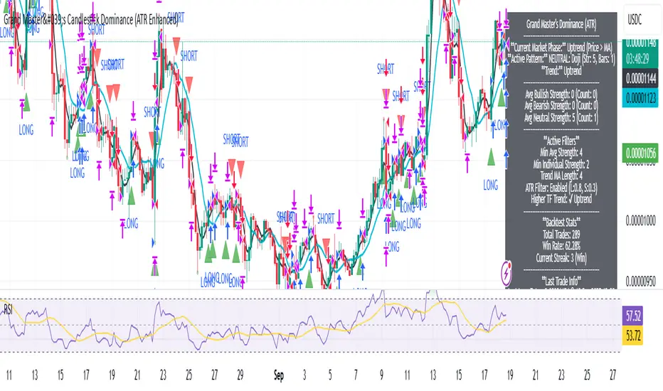
Grand Master's Candlestick Dominance (ATR Enhanced)### Grand Master's Candlestick Dominance (ATR Enhanced)
**Overview**
Unleash the ancient wisdom of Japanese candlestick charting with a modern twist! This comprehensive Pine Script v5 strategy and indicator scans for over 75 classic and advanced candlestick patterns (bullish, bearish, and neutral), assigning dynamic strength scores (1-10) to each for precise signal filtering. Enhanced with Average True Range (ATR) for volatility-aware body size validation, it dominates the markets by combining timeless pattern recognition with robust confirmation layers. Whether used as a backtestable strategy or visual indicator, it empowers traders to spot high-probability reversals, continuations, and indecision setups with surgical accuracy.
Inspired by Steve Nison's *Japanese Candlestick Charting Techniques*, this tool elevates pattern analysis beyond basics—think Hammers, Engulfing patterns, Morning Stars, and rare gems like Abandoned Baby or Concealing Baby Swallow—all consolidated into intelligent arrays for real-time averaging and prioritization.
**Key Features**
- **Extensive Pattern Library**:
- **Bullish (25+ patterns)**: Hammer (8.0), Bullish Engulfing (10.0), Morning Star (7.0), Three White Soldiers (9.0), Dragonfly Doji (8.0), and more (e.g., Rising Three, Unique Three River Bottom).
- **Bearish (25+ patterns)**: Hanging Man (8.0), Bearish Engulfing (10.0), Evening Star (7.0), Three Black Crows (9.0), Gravestone Doji (8.0), and exotics like Upside Gap Two Crows or Stalled Pattern.
- **Neutral/Indecision (34+ patterns)**: Doji variants (Long-Legged, Four Price), Spinning Tops, Harami Crosses, and multi-bar setups like Upside Tasuki Gap or Advancing Block.
Each pattern includes duration tracking (1-5 bars) and ATR-adjusted body/shadow criteria for relevance in volatile conditions.
- **Smart Confirmation Filters** (All Toggleable):
- **Trend Alignment**: 20-period SMA (customizable) ensures entries align with the prevailing trend; optional higher timeframe (e.g., Daily) MA crossover for multi-timeframe confluence.
- **Support/Resistance (S/R)**: Pivot-based levels with 0.01% tolerance to confirm bounces or breaks.
- **Volume Surge**: 20-period volume MA with 1.5x spike multiplier to validate momentum.
- **ATR Body Sizing**: Filters small bodies (<0.3x ATR) and long bodies (>0.8x ATR) for context-aware pattern reliability.
- **Follow-Through**: Ensures post-pattern confirmation via bullish/bearish closes or closes beyond prior bars.
Minimum average strength (default 7.0) and individual pattern thresholds (5.0) prevent weak signals.
- **Entry & Exit Logic**:
- **Long Entry**: Bullish average strength ≥7.0 (outweighing bearish), uptrend, volume spike, near support, follow-through, and HTF alignment.
- **Short Entry**: Mirror for bearish dominance in downtrends near resistance.
- **Exits**: Bearish/neutral shift, or fixed TP (5%) / SL (2%)—pyramiding disabled, 10% equity sizing.
- Backtest range: Jan 1, 2020 – Dec 31, 2025 (editable). Initial capital: $10,000.
- **Interactive Dashboard** (Top-Right Panel):
Real-time insights including:
- Market phase (e.g., "Bullish Phase (Avg Str: 8.2)"), active pattern (e.g., "BULLISH: Bullish Engulfing (Str: 10.0, Bars: 2)"), and trend status.
- Strength breakdowns (Bull/Bear/Neutral counts & averages).
- Filter status (e.g., "Volume: ✔ Spike", "ATR: Enabled (L:0.8, S:0.3)").
- Backtest stats: Total trades, win rate, streak, and last entry/exit details (price & timestamp).
Toggle mode: Strategy (live trades) or Indicator (signals only).
- **Advanced Alerts** (15+ Toggleable Types):
Set up via TradingView's "Any alert() function call" for bar-close triggers:
- Entry/Exit signals with strength & pattern details.
- Strong patterns (≥2 bullish/bearish), neutral indecision, volume spikes.
- S/R breakouts, HTF reversals, high-confidence singles (≥8.0 strength).
- Conflicting signals, MA crossovers, ATR volatility bursts, multi-bar completions.
Example: "STRONG BULLISH PATTERN detected! Strength: 9.5 | Top Pattern: Three White Soldiers | Trend: Up".
**Customization & Usage Tips**
- **Inputs Groups**: Strategy toggles, confirmations, exits, backtest dates, and 15+ alert switches—all intuitively grouped.
- **Optimization**: Tune min strengths for aggressive (lower) or conservative (higher) trading; enable/disable filters to suit your style (e.g., disable S/R for scalping).
- **Best For**: Forex, stocks, crypto on 1H–Daily charts. Test on historical data to refine TP/SL.
- **Limitations**: No external data installs; relies on built-in TA functions. Patterns are probabilistic—combine with your risk management.
Master the candles like a grandmaster. Deploy on TradingView, backtest relentlessly, and let dominance begin! Questions? Drop a comment.
*Version: 1.0 | Updated: September 2025 | Credits: Built on Pine Script v5 with nods to Nison's timeless techniques.*
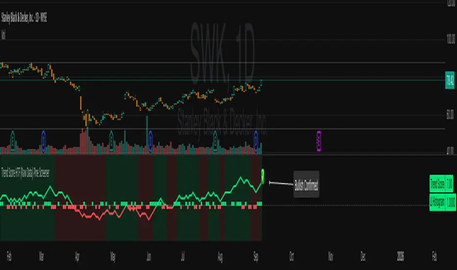
Trend Score HTF (Raw Data) Pine Screener📘 Trend Score HTF (Raw Data) Pine Screener — Indicator Guide
This indicator tracks price action using a custom cumulative Trend Score (TS) system. It helps you visualize trend momentum, detect early reversals, confirm direction changes, and screen for entries across large watchlists like SPX500 using TradingView’s Pine Script Screener (beta).
⸻
🔧 What This Indicator Does
• Assigns a +1 or -1 score when price breaks the previous high or low
• Accumulates these scores into a real-time tsScore
• Detects early warnings (primed flips) and trend changes (confirmed flips)
• Supports alerts and labels for visual and automated trading
• Designed to work inside the Pine Screener so you can filter hundreds of tickers live
⸻
⚙️ Recommended Settings (for Beginners)
When adding the indicator to your chart:
Go to the “Inputs” tab at the top of the settings panel.
Then:
• Uncheck “Confirm flips on bar close”
• Check “Accumulate TS Across Flips? (ON = non-reset, OFF = reset)”
This setup allows you to see trend changes immediately without waiting for bar closes and lets the trend score build continuously over time, making it easier to follow long trends.
⸻
🧠 Core Logic
Start Date
Select a meaningful historical start date — for example: 2020-01-01. This provides long-term context for trend score calculation.
Per-Bar Delta (Δ) Calculation
The indicator scores each bar based on breakout behavior:
If the bar breaks only the previous high, Δ = +1
If it breaks only the previous low, Δ = -1
If it breaks both the high and low, Δ = 0
If it breaks neither, Δ = 0
This filters out wide-range or indecisive candles during volatility.
Cumulative Trend Score
Each bar’s delta is added to the running tsScore.
When it rises, bullish pressure is building.
When it falls, bearish pressure is increasing.
Trend Flip Logic
A bullish flip happens when tsScore rises by +3 from the lowest recent point.
A bearish flip happens when tsScore falls by -3 from the highest recent point.
These flips update the active trend direction between bullish and bearish.
⸻
⚠️ What Is a “Primed” Flip?
A primed flip is a signal that the current trend is about to flip — just one point away.
A primed bullish flip means the trend is currently bearish, but the tsScore only needs +1 more to flip. If the next bar breaks the previous high (without breaking the low), it will trigger a bullish flip.
A primed bearish flip means the trend is currently bullish, but the tsScore only needs -1 more to flip. If the next bar breaks the previous low (without breaking the high), it will trigger a bearish flip.
Primed flips are plotted one bar ahead of the current bar. They act like forecasts and give you a head start.
⸻
✅ What Is a “Confirmed” Flip?
A confirmed flip is the first bar of a new trend direction.
A confirmed bullish flip appears when a bearish trend officially flips into a new bullish trend.
A confirmed bearish flip appears when a bullish trend officially flips into a new bearish trend.
These signals are reliable and great for entries, trend filters, or reversals.
⸻
🖼 Visual Cues
The trend score (tsScore) line shows the accumulated trend strength.
A Δ histogram shows the daily price contribution: +1 for breaking highs, -1 for breaking lows, 0 otherwise.
A green background means the chart is in a bullish trend.
A red background means the chart is in a bearish trend.
A ⬆ label signals a primed bullish flip is possible on the next bar.
A ⬇ label signals a primed bearish flip is possible on the next bar.
A ✅ means a bullish flip just confirmed.
A ❌ means a bearish flip just confirmed.
⸻
🔔 Alerts You Can Use
The indicator includes these built-in alerts:
• Primed Bullish Flip — watch for possible bullish reversal tomorrow
• Primed Bearish Flip — watch for possible bearish reversal tomorrow
• Bullish Confirmed — official entry into new uptrend
• Bearish Confirmed — official entry into new downtrend
You can set these alerts in TradingView to monitor across your chart or watchlist.
⸻
📈 How to Use in TradingView Pine Screener
Step 1: Create your own watchlist — for example, SPX500
Step 2: Favorite this indicator so it shows up in the screener
Step 3: Go to TradingView → Products → Screeners → Pine (Beta)
Step 4: Select this indicator and choose a condition, like “Bullish Confirmed”
Step 5: Click Scan
You’ll instantly see stocks that just flipped trends or are close to doing so.
⸻
⏰ When to Use the Screener
Use this screener after market close or before the next open to avoid intraday noise.
During the day, if a candle breaks both the high and low, the delta becomes 0, which may cancel a flip or primed signal.
Results during regular trading hours can change frequently. For best results, scan during stable periods like pre-market or after-hours.
⸻
🧪 Real-World Examples
SWK
NVR
WMT
UNH
Each of these examples shows clean, structured trend transitions detected in advance or confirmed with precision.
PLTR: complicated case primed for bullish (but we don't when it will flip)
⚠️ Risk Disclaimer & Trend Context
A confirmed bullish signal does not guarantee an immediate price increase. Price may continue to consolidate or even pull back after a bullish flip.
Likewise, a primed bullish signal does not always lead to confirmation. It simply means the conditions are close — but if the next bar breaks both the high and low, or breaks only the low, the flip will be canceled.
On the other side, a confirmed bearish signal does not mean the market will crash. If the overall trend is bullish (for example, tsScore has been rising for weeks), then a bearish flip may just represent a short-term pullback — not a trend reversal.
You always need to consider the overall market structure. If the long-term trend is bullish, it’s usually smarter to wait for bullish confirmation signals. Bearish flips in that context are often just dips — not opportunities to short.
This indicator gives you context, not predictions. It’s a tool for alignment — not absolute outcomes. Use it to follow structure, not fight it.
Eureka & Phoenix Thrust — NYSE (90% Breadth Days)🚀Eureka & Phoenix Thrust Indicator (NYSE Breadth)
Overview
This free indicator highlights rare but powerful breadth thrust days on the NYSE that can mark important turning points in the market.
It automatically detects both:
📈 Eureka Thrust (90% Up Day)
– At least 90% of NYSE issues advance and at least 90% of NYSE volume is advancing.
– Often signals broad-based institutional buying and strong market demand.
📉 Phoenix Thrust (90% Down Day)
– At least 90% of NYSE issues decline and at least 90% of NYSE volume is declining.
– Reflects broad institutional selling or panic, sometimes marking capitulation lows.
Both signal types were popularized by Lowry’s Research and O’Neil/IBD market models.
Notes
Eureka Thrusts are bullish confirmation signals, especially when clustered.
Phoenix Thrusts often mark panic selling — bearish in the short term, but can precede market bottoms if followed by Eurekas.
These events are rare. You may need to scroll back in history (e.g., March 2020, 2008, 1987) to see them in action.
Disclaimer
This tool is for educational and informational purposes only.
It is not financial advice. Always do your own research and risk management before making trading or investment decisions.
