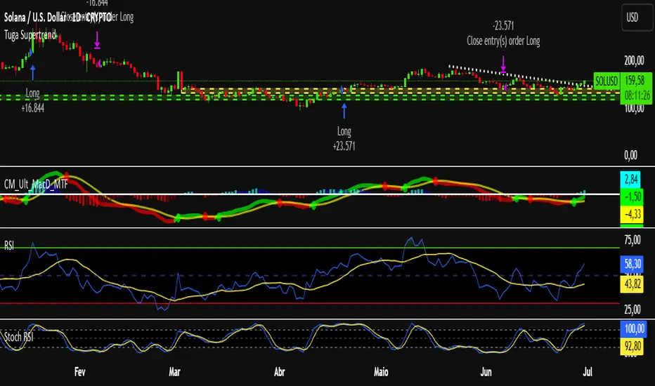
Tuga SupertrendDescription
This strategy uses the Supertrend indicator enhanced with commission and slippage filters to capture trends on the daily chart. It’s designed to work on any asset but is especially effective in markets with consistent movements.
Use the date inputs to set the backtest period (default: from January 1, 2018, through today, June 30, 2025).
The default input values are optimized for the daily chart. For other timeframes, adjust the parameters to suit the asset you’re testing.
Release Notes
June 30, 2025
• Updated default backtest period to end on June 30, 2025.
• Default commission adjusted to 0.1 %.
• Slippage set to 3 ticks.
• Default slippage set to 3 ticks.
• Simplified the strategy name to “Tuga Supertrend”.
Default Parameters
Parameter Default Value
Supertrend Period 10
Multiplier (Factor) 3
Commission 0.1 %
Slippage 3 ticks
Start Date January 1, 2018
End Date June 30, 2025
"山子高科2025年一季度财务报告关键指标" için komut dosyalarını ara
Gold and Bitcoin: The Evolution of Value!The Eternal Luster of Gold
In the dawn of time, when the earth was young and rivers whispered secrets to the stones, a wanderer named Elara found a gleam in the silt of a sun-kissed stream. It was pure gold, radiant like a captured star fallen from the heavens. She held it in her palm, feeling its warmth pulse like a heartbeat, and in that moment, humanity’s soul awakened to the allure of eternity.
As seasons turned to centuries, gold wove itself into the story of empires. In ancient Egypt, pharaohs crowned themselves with its glow, believing it to be the flesh of gods. It built pyramids that reached for the sky and tombs that guarded kings forever. Across the sands in Mesopotamia, merchants traded it for spices and silks, its weight a promise of power and trust.
Translation moment: Gold became the first universal symbol of value. People trusted it more than words or promises because it did not rust, fade, or vanish.
The Greeks saw in gold not only wealth but wisdom, the symbol of the sun’s eternal fire. Alexander the Great carried it across the continent, forging an empire of golden threads. Rome rose on its back, minting coins whose clink echoed through history.
Through the ages, gold endured the rush of California’s dreamers, the halls of Versailles, and the quiet vaults of modern fortunes. It has been both a curse and a blessing, the fuel of wars and the gift of love, whispering of beauty’s fragility and the human desire for something that lasts beyond the grave. In its shine, we see ourselves fragile yet forever chasing light.
The Digital Dawn of Bitcoin
Centuries later, under the glow of computer screens, a visionary named Satoshi dreamed of a new gold born not from the earth but from the ether of ideas. Bitcoin appeared in 2009 amid a world weary of banks and broken trust.
Like gold’s ancient gleam, Bitcoin was mined not with picks but with puzzles solved by machines. It promised freedom, a currency without kings, flowing from person to person, unbound by borders or empires.
Translation moment: Bitcoin works like digital gold. Instead of digging the ground, miners use computers to solve problems and unlock new coins. No one controls it, and that is what makes it powerful.
Through doubt and frenzy, it rose as a beacon for those seeking sovereignty in a digital world. Its volatility became its soul, a reminder that true value is built on belief. Bitcoin speaks to ingenuity and rebellion, a star of code guiding us toward a future where wealth is weightless yet profoundly honest.
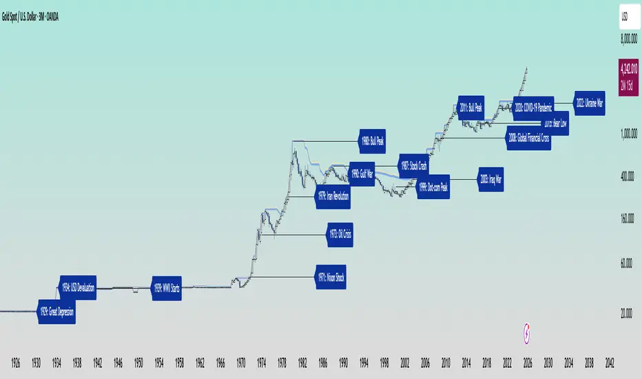
Gold’s Cycles: Echoes of War and Crisis
In the early 20th century, gold was held under fixed prices until the Great Depression of 1929 shattered these illusions. The 1934 dollar devaluation lifted it from 20.67 to 35, restoring faith amid despair. When World War II erupted in 1939, gold’s role as a refuge was muted by controls, yet it quietly held its place as the world’s silent guardian.
The 1970s awakened its wild spirit. The Nixon Shock of 1971 freed gold from 35, sparking a bull run during the 1973 Oil Crisis. The 1979 Iranian Revolution led to a 1980 peak of 850, a leap of more than 2,000 percent, as investors sought safety from the chaos.
Translation moment: When fear rises, people rush to gold. Every major war or economic crisis has sent gold upward because it feels safe when paper money loses trust.
The 1987 stock crash caused brief dips, but the 1990 Gulf War reignited its glow. Around 2000, after the Dot-com Bust, gold found new life, climbing from $ 270 to over $1,900 during the 2008 Financial Crisis. It dipped to 1050 in 2015, then surged again past 2000 during the 2020 pandemic.
The 2022 Ukraine War added another chapter with prices climbing above 2700 by 2025. Across a century of crises, gold has risen whenever fear tested humanity’s resolve, teaching patience and fortitude through its quiet endurance.
Bitcoin’s Cycles: Echoes of Innovation and Crisis
Born from the ashes of the 2008 Financial Crisis, Bitcoin began its story at mere cents. It traded below $1 until 2011, when it reached $30 before crashing by 90 percent following the MTGOX collapse.
In 2013, it soared to 1242 only to fall again to 200 in 2015 as regulations tightened. The 2017 bull run lifted it to nearly 20000 before another long winter brought it to 3200 in 2018. Each fall taught resilience, each rise renewed belief.
During the 2020 pandemic, it fell below 5000 before rallying to 69000 in 2021. The Ukraine War and the FTX collapse of 2022 brought it down to 16000, but also proved its role in humanitarian aid. By 2024, the halving and ETF approvals helped it break 100000, marking Bitcoin’s rise as digital gold.
Translation moment: Bitcoin’s rhythm follows four-year halving cycles when mining rewards are cut in half. This keeps supply limited, which often triggers new bull runs as demand returns.
Every four years, it's halving cycles 2012, 2016, 2020, 2024, fueling new waves of adoption and correction. Bitcoin grows strongest in times of uncertainty, echoing humanity’s drive to evolve beyond limits.
The Harmony of Gold and Bitcoin Modern Parallels
In today’s markets, gold’s ancient glow meets Bitcoin’s electric pulse. As of October 17, 2025, their correlation stands near 0.85, close to its historic high of 0.9. Both rise as guardians against inflation and the erosion of trust in the dollar.
Gold trades near 4310 per ounce a record high while Bitcoin hovers around 104700 showing brief fractures in their unity. Gold offers the comfort of touch while Bitcoin provides the thrill of code. Together, they reflect fear and hope, the twin emotions that drive every market.
Translation moment: A correlation of 0.85 means they often move in the same direction. When fear or inflation rises, both gold and Bitcoin tend to rise in tandem.
Analysts warn of bubbles in stocks, gold, and crypto, yet optimism remains for Bitcoin’s growth through 2026, while gold holds its defensive strength.
Gold carries risks of storage cost and theft, but steadiness in chaos. Bitcoin carries volatility and regulatory challenges, but it also offers unmatched innovation and reach. One is the anchor, the other the dream, and both reward those who hold conviction through uncertainty.
Epilogue: The Timeless Balance
Gold and Bitcoin form a bridge between the ancient and the future. Gold, the earth’s eternal treasure, stands as a symbol of stability and truth. Bitcoin, the digital heir, shines with the spark of innovation and freedom.
Experts view gold as the ultimate inflation hedge, forged in fire and tested over centuries. They see Bitcoin as its digital counterpart, scarce by code and limitless in reach.
Gold’s weight grounds us in reality while Bitcoin’s light expands our imagination. In 2025, as gold surpasses $4,346 and Bitcoin hovers near $105,000, the wise investor sees not rivals but reflections.
Translation moment: Gold reminds us to protect what we have. Bitcoin reminds us to dream of what could be. Together, they balance caution and courage, the two forces every generation must master.
One whispers of legacy, the other of evolution, yet together they tell humanity’s oldest story, our unending quest to preserve value against time and to chase the light that never fades.
🙏 I ask (Allah) for guidance and success. 🤲
Bitcoin Cycle History Visualization [SwissAlgo]BTC 4-Year Cycle Tops & Bottoms
Historical visualization of Bitcoin's market cycles from 2010 to present, with projections based on weighted averages of past performance.
-----------------------------------------------------------------
CALCULATION METHODOLOGY
Why Bottom-to-Bottom Cycle Measurement?
This indicator defines cycles as bottom-to-bottom periods. This is one of several valid approaches to Bitcoin cycle analysis:
- Focuses on market behavior (price bottoms) rather than supply schedule events (halving-to-halving)
- Bottoms may offer good reference points for some analytical purposes
- Tops tend to be extended periods that are harder to define precisely
- Aligns with how some traditional asset cycles are measured and the timing observed in the broader "risk-on" assets category
- Halving events are shown separately (yellow backgrounds) for reference
- Neither halving-based nor bottom-based measurement is inherently superior
Different analysts prefer different cycle definitions based on their analytical goals. This approach prioritizes observable market turning points.
Cycle Date Definitions
- Approximate monthly ranges used for each event (e.g., Nov 2022 bottom = Nov 1-30, 2022)
- Cycle 1: Jul 2010 bottom → Jun 2011 top → Nov 2011 bottom
- Cycle 2: Nov 2011 bottom → Dec 2013 top → Jan 2015 bottom
- Cycle 3: Jan 2015 bottom → Dec 2017 top → Dec 2018 bottom
- Cycle 4: Dec 2018 bottom → Nov 2021 top → Nov 2022 bottom
- Future cycles will be added as new top/bottom dates become firm
Duration Calculations
- Days = timestamp difference converted to days (milliseconds ÷ 86,400,000)
- Bottom → Top: days from cycle bottom to peak
- Top → Bottom: days from peak to next cycle bottom
- Bottom → Bottom: full cycle duration (sum of above)
Price Change Calculations
- % Change = ((New Price - Old Price) / Old Price) × 100
- Example: $200 → $19,700 = ((19,700 - 200) / 200) × 100 = 9,750% gain
- Approximate historical prices used (rounded to significant figures)
Weighted Average Formula
Recent cycles weighted more heavily to reflect the evolved market structure:
- Cycle 1 (2010-2011): EXCLUDED (too early-stage, tiny market cap)
- Cycle 2 (2011-2015): Weight = 1x
- Cycle 3 (2015-2018): Weight = 3x
- Cycle 4 (2018-2022): Weight = 5x
Formula: Weighted Avg = (C2×1 + C3×3 + C4×5) / (1+3+5)
Example for Bottom→Top days: (761×1 + 1065×3 + 1066×5) / 9 = 1,032 days
Projection Method
- Projected Top Date = Nov 2022 bottom + weighted avg Bottom→Top days
- Projected Bottom Date = Nov 2022 bottom + weighted avg Bottom→Bottom days
- Current days elapsed compared to weighted averages
- Warning symbol (⚠) shown when the current cycle exceeds the historical average
Technical Implementation
- Historical cycle dates are hardcoded (not algorithmically detected)
- Dates represent approximate monthly ranges for each event
- The indicator will be updated as the Cycle 5 top and bottom dates become confirmed
- Updates require manual code maintenance - not automatic
- Users should verify they're using the latest version for current cycle data
-----------------------------------------------------------------
FEATURES
- Background highlights for historical tops (red), bottoms (green), and halving events (yellow)
- Data table showing cycle durations and price changes
- Visual cycle boundary boxes with subtle coloring
- Projected timeframes displayed as dashed vertical lines
- Toggle on/off for each visual element
- Customizable background colors
-----------------------------------------------------------------
DISPLAY SETTINGS
- Show/hide cycle tops, bottoms, halvings, data table, and cycle boxes
- Customizable background colors for each event type
- Clean, institutional-grade visual design suitable for analysis
UPDATES & MAINTENANCE
This indicator is maintained as new cycle events occur. When Cycle 5's top and bottom are confirmed with sufficient time elapsed, the code and projections will be updated accordingly. Check for the latest version periodically.
OPEN SOURCE
Code available for review, modification, and improvement. Educational transparency is prioritized.
-----------------------------------------------------------------
IMPORTANT LIMITATIONS
⚠ EXTREMELY SMALL SAMPLE SIZE
Based on only 4 complete cycles (2011-2022). In statistical analysis, this is insufficient for reliable predictions.
⚠ CHANGED MARKET STRUCTURE
Bitcoin's market has fundamentally evolved since early cycles:
- 2010-2015: Tiny market cap, retail-only, unregulated
- 2024-2025: Institutional adoption, spot ETFs, regulatory frameworks, macro correlation
The environment that created past patterns no longer exists in the same form.
⚠ NO PREDICTIVE GUARANTEE
Historical patterns can and do break. Market cycles are not laws of physics. Past performance does not guarantee future results. The next cycle may not follow historical averages.
⚠ LENGTHENING CYCLE THEORY
Some analysts believe cycles are extending over time (diminishing returns, maturing market). If true, simple averaging underestimates future cycle lengths.
⚠ SELF-FULFILLING PROPHECY RISK
The halving narrative may be partially circular - it works because people believe it works. Sufficient changes in market structure or participant behavior can invalidate the pattern.
⚠ APPROXIMATE DATA
Historical prices rounded to significant figures. Exact bottom/top dates vary by exchange. Month-long ranges are used for simplicity.
EDUCATIONAL USE ONLY
This indicator is designed for historical analysis and understanding Bitcoin's past behavior. It is NOT:
- Trading advice or financial recommendations
- A guarantee or prediction of future price movements
- Suitable as a sole basis for investment decisions
- A replacement for fundamental or technical analysis
The projections show "what if the pattern continues exactly" - not "what will happen."
Always conduct independent research, understand the risks, and consult qualified financial advisors before making investment decisions. Only invest what you can afford to lose.

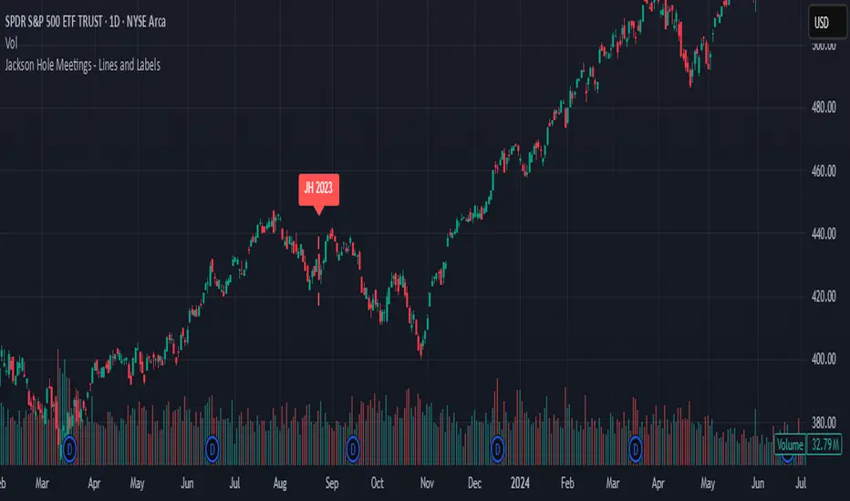
Jackson Hole Meetings - Lines and LabelsThis TradingView Pine Script indicator marks the dates of the Federal Reserve’s annual Jackson Hole Economic Symposium meetings on your chart. For each meeting date from 2020 through 2025, it draws a red dashed vertical line directly on the corresponding daily bar. Additionally, it places a label above the bar indicating the year of the meeting (e.g., "JH 2025").
Features:
Marks all known Jackson Hole meeting dates from 2020 to 2025.
Draws a vertical dashed line on each meeting day for clear visual identification.
Displays a label above the candle with the meeting year.
Works best on daily timeframe charts.
Helps traders quickly spot potential market-moving events related to Jackson Hole meetings.
Use this tool to visually correlate price action with these key Federal Reserve events and enhance your trading analysis.
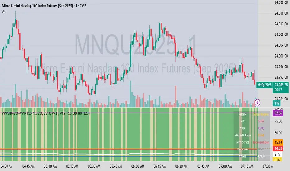
VWATR + VIX + VVIX Trend Regime### 🤖 VWATR + VIX + VVIX Trend Regime — Your Ultimate Volatility Dashboard! 📊
This isn't just another indicator; it's a comprehensive dashboard that brings together everything you need to understand market volatility focused on Futures. It merges price-based movement with market-wide fear and sentiment, giving you a powerful edge in your trading and risk management. Think of it as your personal volatility sidekick, ready to help you navigate market uncertainty like a pro!
***
### ✨ What's Inside?
* **VWATR (Volume-Weighted ATR):** A super-smart measure of price movement that pays close attention to where the big money is flowing.
* **VIX (The "Fear Gauge"):** Tracks the expected volatility of the S&P 500, essentially telling you how nervous the market is feeling.
* **VVIX (The "VIX of VIX"):** This one's for the pros! It measures how volatile the VIX itself is, giving you an early heads-up on potential fear spikes.
* **VX Term Structure:** A clever way to see if traders are preparing for a crisis. It compares the two nearest VIX futures to spot a rare signal called "backwardation."
* **Z-Scores:** It helps you spot when VIX and VVIX are at historic highs or lows, making it easier to predict when things might return to normal.
* **Divergence Score:** A unique tool to flag potential market shifts when the VIX and VVIX start moving in completely different directions.
* **Regime Classification:** The script automatically labels the market as "Full Panic," "Known Crisis," "Surface Calm," "Stress," or "Normal," so you always know where you stand.
* **Gradient Bars:** A visual treat! The background of your chart changes color to reflect real-time volatility shifts, giving you an instant feel for the market's mood.
* **Alerts:** Get push notifications on your phone for key events like "Full Panic" or "Backwardation" so you never miss a beat.
***
### 📝 Panel/Table Outputs
This is your mission control! The on-screen table gives you a clean summary of the current market regime, VIX and VVIX values, their ratios, term structure, Z-scores, and signals. Everything you need, right where you can see it.
***
### 🚀 How to Get Started
1. **Check your data:** You'll need access to real-time data for VIX, VVIX, VX1!, and VX2!. A paid subscription might be necessary for this.
2. **Add it to your chart:** Use the indicator on any chart (we've set it to `overlay=false`) to get your full volatility dashboard.
3. **Tweak it to perfection:** Head over to the Settings panel to customize the thresholds, colors, and your all-important "Jolt Value."
4. **Start trading smarter:** Use the dashboard to inform your trades, hedge your portfolio, and manage risk with confidence.
***
### ⚙️ Customization & Key Settings
* `showVWATR`: Toggle your price-volatility metric on or off.
* `showExpectedVol`: See the expected volatility as a percentage of the current price.
* `joltLevel`: This is a very important line on your chart! It's your personal trigger for when volatility is getting a little too wild. More on this below.
* `enableGradientBars`: Turn the awesome colored background on or off.
* `enableTable`: Hide or show your information table.
* `VIX/VVIX/VX1!/VX2! symbols`: If your broker uses different symbols for these, you can change them here.
* `VIX/VVIX thresholds`: Adjust these levels to fine-tune the indicator to your personal risk tolerance.
***
### 💡 Jolt Value: A Quick Guide for Smart Traders 🧠
The **jolt value** is your personal tripwire for volatility. Think of it as a warning light on your car's dashboard. You set the level, and when volatility (VWATR) crosses that line, you get an instant signal that something interesting is happening.
**How to Set Your Jolt Value:**
The ideal jolt value is dynamic. You want to keep it just a little above the current VIX level to stay alert without getting too many false alarms.
| Current VIX Level | Market Regime | Recommended Jolt Value |
| :--- | :--- | :--- |
| Under 15 | Calm/Complacent | 15–16 |
| 15–20 | Typical/Normal | 16–18 |
| 20–30 | Cautious/Active | 18–22 |
| Over 30 | Stress/Panic | 30+ |
**A Pro Tip for August 2025:** Since the VIX is hovering around 14.7, setting your jolt value to **16.5** is a great starting point for keeping an eye on things. If the VIX starts to climb above 20, you should adjust your jolt level to match the new reality.
***
### ⚠️ Important Things to Note
* You might experience some data delays if you're not on a paid TradingView plan or your broker does not provide real-time data for the VIX also VIX is only active during NY session, so it's not advised to use it outside of normal trading hours!
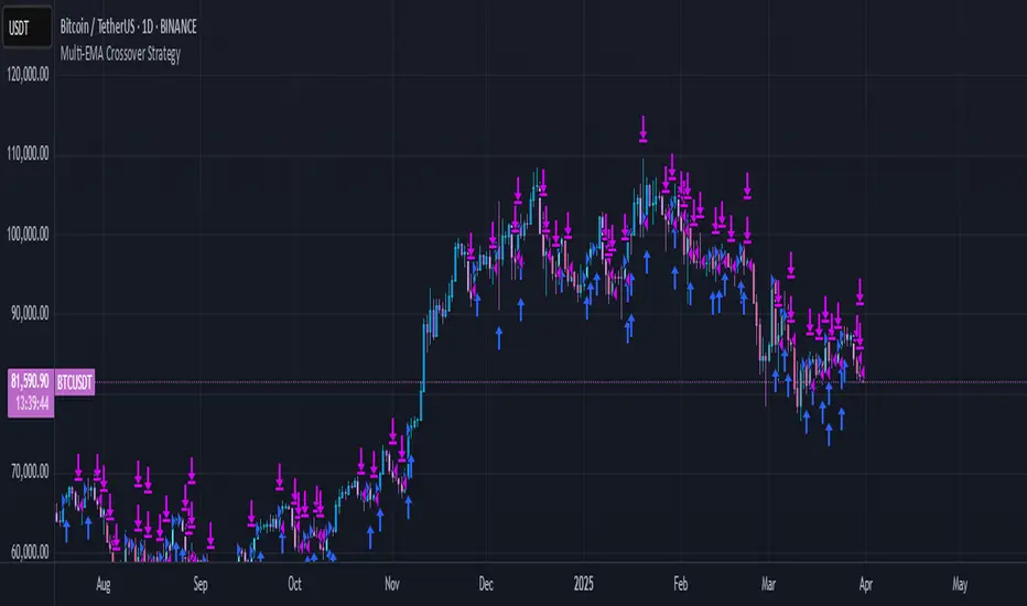
Multi-EMA Crossover StrategyMulti-EMA Crossover Strategy
This strategy uses multiple exponential moving average (EMA) crossovers to identify bullish trends and execute long trades. The approach involves progressively stronger signals as different EMA pairs cross, indicating increasing bullish momentum. Each crossover triggers a long entry, and the intensity of bullish sentiment is reflected in the color of the bars on the chart. Conversely, bearish trends are represented by red bars.
Strategy Logic:
First Long Entry: When the 1-day EMA crosses above the 5-day EMA, it signals initial bullish momentum.
Second Long Entry: When the 3-day EMA crosses above the 10-day EMA, it confirms stronger bullish sentiment.
Third Long Entry: When the 5-day EMA crosses above the 20-day EMA, it indicates further trend strength.
Fourth Long Entry: When the 10-day EMA crosses above the 40-day EMA, it suggests robust long-term bullish momentum.
The bar colors reflect these conditions:
More blue bars indicate stronger bullish sentiment as more short-term EMAs are above their longer-term counterparts.
Red bars represent bearish conditions when short-term EMAs are below longer-term ones.
Example: Bitcoin Trading on a Daily Timeframe
Bullish Scenario:
Imagine Bitcoin is trading at $30,000 on March 31, 2025:
First Signal: The 1-day EMA crosses above the 5-day EMA at $30,000. This suggests initial upward momentum, prompting a small long entry.
Second Signal: A few days later, the 3-day EMA crosses above the 10-day EMA at $31,000. This confirms strengthening bullish sentiment; another long position is added.
Third Signal: The 5-day EMA crosses above the 20-day EMA at $32,500, indicating further upward trend development; a third long entry is executed.
Fourth Signal: Finally, the 10-day EMA crosses above the 40-day EMA at $34,000. This signals robust long-term bullish momentum; a fourth long position is entered.
Bearish Scenario:
Suppose Bitcoin reverses from $34,000 to $28,000:
The 1-day EMA crosses below the 5-day EMA at $33,500.
The 3-day EMA dips below the 10-day EMA at $32,000.
The 5-day EMA falls below the 20-day EMA at $30,000.
The final bearish signal occurs when the 10-day EMA drops below the 40-day EMA at $28,000.
The bars turn increasingly red as bearish conditions strengthen.
Advantages of This Strategy:
Progressive Confirmation: Multiple crossovers provide layered confirmation of trend strength.
Visual Feedback: Bar colors help traders quickly assess market sentiment and adjust positions accordingly.
Flexibility: Suitable for trending markets like Bitcoin during strong rallies or downturns.
Limitations:
Lagging Signals: EMAs are lagging indicators and may react slowly to sudden price changes.
False Breakouts: Crossovers in choppy markets can lead to whipsaws or false signals.
This strategy works best in trending markets and should be combined with additional risk management techniques, e.g., stop loss or optimal position sizes (Kelly Criterion).
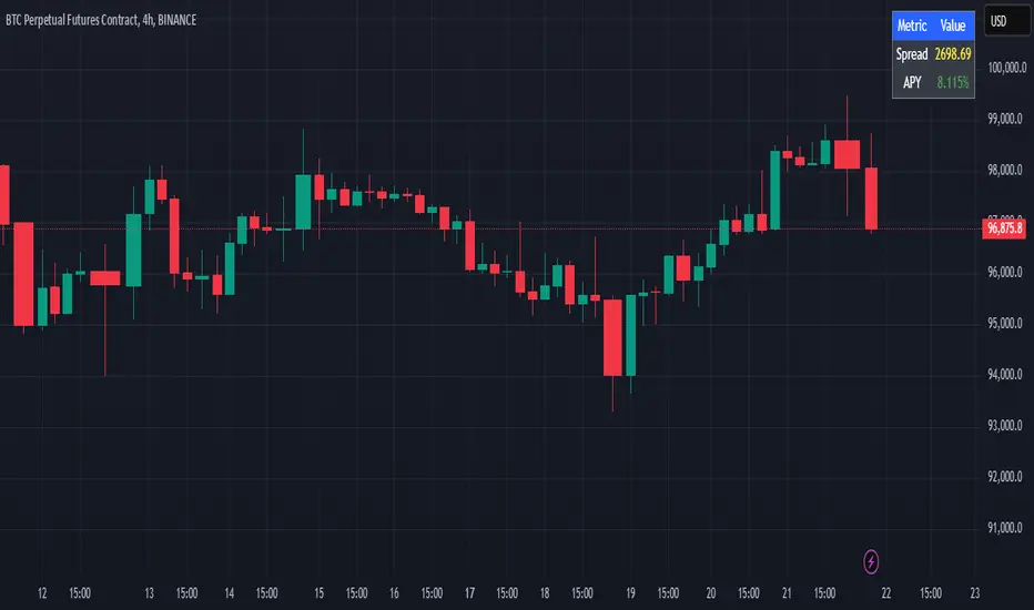
Cash And Carry Arbitrage BTC Compare Month 6 by SeoNo1Detailed Explanation of the BTC Cash and Carry Arbitrage Script
Script Title: BTC Cash And Carry Arbitrage Month 6 by SeoNo1
Short Title: BTC C&C ABT Month 6
Version: Pine Script v5
Overlay: True (The indicators are plotted directly on the price chart)
Purpose of the Script
This script is designed to help traders analyze and track arbitrage opportunities between the spot market and futures market for Bitcoin (BTC). Specifically, it calculates the spread and Annual Percentage Yield (APY) from a cash-and-carry arbitrage strategy until a specific expiry date (in this case, June 27, 2025).
The strategy helps identify profitable opportunities when the futures price of BTC is higher than the spot price. Traders can then buy BTC in the spot market and short BTC futures contracts to lock in a risk-free profit.
1. Input Settings
Spot Symbol: The real-time BTC spot price from Binance (BTCUSDT).
Futures Symbol: The BTC futures contract that expires in June 2025 (BTCUSDM2025).
Expiry Date: The expiration date of the futures contract, set to June 27, 2025.
These inputs allow users to adjust the symbols or expiry date according to their trading needs.
2. Price Data Retrieval
Spot Price: Fetches the latest closing price of BTC from the spot market.
Futures Price: Fetches the latest closing price of BTC futures.
Spread: The difference between the futures price and the spot price (futures_price - spot_price).
The spread indicates how much higher (or lower) the futures price is compared to the spot market.
3. Time to Maturity (TTM) and Annual Percentage Yield (APY) Calculation
Current Date: Gets the current timestamp.
Time to Maturity (TTM): The number of days left until the futures contract expires.
APY Calculation:
Formula:
APY = ( Spread / Spot Price ) x ( 365 / TTM Days ) x 100
This represents the annualized return from holding a cash-and-carry arbitrage position if the trader buys BTC at the spot price and sells BTC futures.
4. Display Information Table on the Chart
A table is created on the chart's top-right corner showing the following data:
Metric: Labels such as Spread and APY
Value: Displays the calculated spread and APY
The table automatically updates at the latest bar to display the most recent data.
5. Alert Condition
This sets an alert condition that triggers every time the script runs.
In practice, users can modify this alert to trigger based on specific conditions (e.g., APY exceeds a threshold).
6. Plotting the APY and Spread
APY Plot: Displays the annualized yield as a blue line on the chart.
Spread Plot: Visualizes the futures-spot spread as a red line.
This helps traders quickly identify arbitrage opportunities when the spread or APY reaches desirable levels.
How to Use the Script
Monitor Arbitrage Opportunities:
A positive spread indicates a potential cash-and-carry arbitrage opportunity.
The larger the APY, the more profitable the arbitrage opportunity could be.
Timing Trades:
Execute a buy on the BTC spot market and simultaneously sell BTC futures when the APY is attractive.
Close both positions upon futures contract expiry to realize profits.
Risk Management:
Ensure you have sufficient margin to hold both positions until expiry.
Monitor funding rates and volatility, which could affect returns.
Conclusion
This script is an essential tool for traders looking to exploit price discrepancies between the BTC spot market and futures market through a cash-and-carry arbitrage strategy. It provides real-time data on spreads, annualized returns (APY), and visual alerts, helping traders make informed decisions and maximize their profit potential.
Ripple (XRP) Model PriceAn article titled Bitcoin Stock-to-Flow Model was published in March 2019 by "PlanB" with mathematical model used to calculate Bitcoin model price during the time. We know that Ripple has a strong correlation with Bitcoin. But does this correlation have a definite rule?
In this study, we examine the relationship between bitcoin's stock-to-flow ratio and the ripple(XRP) price.
The Halving and the stock-to-flow ratio
Stock-to-flow is defined as a relationship between production and current stock that is out there.
SF = stock / flow
The term "halving" as it relates to Bitcoin has to do with how many Bitcoin tokens are found in a newly created block. Back in 2009, when Bitcoin launched, each block contained 50 BTC, but this amount was set to be reduced by 50% every 210,000 blocks (about 4 years). Today, there have been three halving events, and a block now only contains 6.25 BTC. When the next halving occurs, a block will only contain 3.125 BTC. Halving events will continue until the reward for minors reaches 0 BTC.
With each halving, the stock-to-flow ratio increased and Bitcoin experienced a huge bull market that absolutely crushed its previous all-time high. But what exactly does this affect the price of Ripple?
Price Model
I have used Bitcoin's stock-to-flow ratio and Ripple's price data from April 1, 2014 to November 3, 2021 (Daily Close-Price) as the statistical population.
Then I used linear regression to determine the relationship between the natural logarithm of the Ripple price and the natural logarithm of the Bitcoin's stock-to-flow (BSF).
You can see the results in the image below:
Basic Equation : ln(Model Price) = 3.2977 * ln(BSF) - 12.13
The high R-Squared value (R2 = 0.83) indicates a large positive linear association.
Then I "winsorized" the statistical data to limit extreme values to reduce the effect of possibly spurious outliers (This process affected less than 4.5% of the total price data).
ln(Model Price) = 3.3297 * ln(BSF) - 12.214
If we raise the both sides of the equation to the power of e, we will have:
============================================
Final Equation:
■ Model Price = Exp(- 12.214) * BSF ^ 3.3297
Where BSF is Bitcoin's stock-to-flow
============================================
If we put current Bitcoin's stock-to-flow value (54.2) into this equation we get value of 2.95USD. This is the price which is indicated by the model.
There is a power law relationship between the market price and Bitcoin's stock-to-flow (BSF). Power laws are interesting because they reveal an underlying regularity in the properties of seemingly random complex systems.
I plotted XRP model price (black) over time on the chart.
Estimating the range of price movements
I also used several bands to estimate the range of price movements and used the residual standard deviation to determine the equation for those bands.
Residual STDEV = 0.82188
ln(First-Upper-Band) = 3.3297 * ln(BSF) - 12.214 + Residual STDEV =>
ln(First-Upper-Band) = 3.3297 * ln(BSF) – 11.392 =>
■ First-Upper-Band = Exp(-11.392) * BSF ^ 3.3297
In the same way:
■ First-Lower-Band = Exp(-13.036) * BSF ^ 3.3297
I also used twice the residual standard deviation to define two extra bands:
■ Second-Upper-Band = Exp(-10.570) * BSF ^ 3.3297
■ Second-Lower-Band = Exp(-13.858) * BSF ^ 3.3297
These bands can be used to determine overbought and oversold levels.
Estimating of the future price movements
Because we know that every four years the stock-to-flow ratio, or current circulation relative to new supply, doubles, this metric can be plotted into the future.
At the time of the next halving event, Bitcoins will be produced at a rate of 450 BTC / day. There will be around 19,900,000 coins in circulation by August 2025
It is estimated that during first year of Bitcoin (2009) Satoshi Nakamoto (Bitcoin creator) mined around 1 million Bitcoins and did not move them until today. It can be debated if those coins might be lost or Satoshi is just waiting still to sell them but the fact is that they are not moving at all ever since. We simply decrease stock amount for 1 million BTC so stock to flow value would be:
BSF = (19,900,000 – 1.000.000) / (450 * 365) =115.07
Thus, Bitcoin's stock-to-flow will increase to around 115 until AUG 2025. If we put this number in the equation:
Model Price = Exp(- 12.214) * 114 ^ 3.3297 = 36.06$
Ripple has a fixed supply rate. In AUG 2025, the total number of coins in circulation will be about 56,000,000,000. According to the equation, Ripple's market cap will reach $2 trillion.
Note that these studies have been conducted only to better understand price movements and are not a financial advice.

Multi-Timeframe MACD with Color Mix (Nikko)Multi-Timeframe MACD with Color Mix (Nikko) Indicator
This documentation explains the benefits of the "Multi-Timeframe MACD with Color Mix (Nikko)" indicator for traders and provides easy-to-follow steps on how to use it. Written as of 05:06 AM +07 on Saturday, October 04, 2025, this guide focuses on helping you, as a trader, get the most out of this tool with clear, practical advice before diving into the technical details.
Benefits for Traders
1. Multi-Timeframe Insight
This indicator lets you see momentum trends across 15-minute, 1-hour, 1-day, and 1-week timeframes all on one chart. This big-picture view helps you catch both quick market moves and long-term trends without flipping between charts, saving you time and giving you a fuller understanding of the market.
2. Visual Momentum Representation
The background changes from red to green based on short-term (15m) momentum, giving you a quick, easy-to-see signal—red means bearish (prices might drop), and green means bullish (prices might rise). The histogram uses a mix of red, green, and blue colors to show the combined strength of the 1-hour, 1-day, and 1-week timeframes, helping you spot strong trends at a glance (e.g., a bright mix for strong momentum, darker for weaker).
3. Enhanced Decision-Making
The background and histogram colors work together to confirm trends across different timeframes, making it less likely you’ll act on a false signal. This helps you feel more confident when deciding when to buy, sell, or hold.
4. Proactive Alert System
You can set alerts to notify you when the percentage of bullish timeframes hits your chosen levels (e.g., below 10% for bearish, above 90% for bullish). This keeps you in the loop on big momentum shifts without needing to watch the chart all day—perfect for when you’re busy.
5. Flexibility and Efficiency
You can turn timeframes on or off, adjust settings like speed of the moving averages, and tweak transparency to fit your trading style—whether you’re a fast scalper or a patient swing trader. Everything is shown on one chart, saving you effort, and the colors make it simple to read, even if you’re new to trading.
How to Use It
Getting Started
Add the Indicator: Load the "Multi-Timeframe MACD with Color Mix (Nikko)" onto your TradingView chart using the Pine Script editor or indicator library.
Pick Your Timeframes: Turn on the timeframes that match your trading—use 15m and 1h for quick trades, or 1d and 1w for longer holds—using the enable_15m, enable_1h, enable_1d, enable_1w, and enable_background options.
Reading the Colors
Background Gradient: Watch for red to signal bearish 15m momentum and green for bullish momentum. Adjust the Background_transparency (default 75%, or 25% opacity) if the chart feels too busy—try lowering it to 50 for clearer candlesticks in fast markets.
Histogram and EMA Colors:
The histogram and its Exponential Moving Average (EMA) line show a mix of red (1-week), green (1-day), and blue (1-hour) based on how strong the momentum is in each timeframe.
Brighter colors mean stronger momentum—white (all bright) shows all timeframes are pushing up hard, while darker shades (like gray or black) mean weaker or mixed momentum.
Turn off a timeframe (e.g., enable_1h = false) to see how it changes the color mix and focus on what matters to you.
Setting Alerts
Set Your Levels: Choose a threshold_low (default 10%) and threshold_high (default 90%) based on your comfort zone or past market patterns to catch big turns.
Get Notifications: Use TradingView alerts to get pings when the market hits your set levels, so you can act without staring at the screen.
Practical Tips
Pair with Other Tools: Use it with support/resistance lines or the RSI to double-check your moves and build a solid plan.
Tweak Settings: Adjust fast_length, slow_length, and signal_smoothing to match your asset’s speed, and bump up the lookback (default 50) for steadier trends in wild markets.
Practice First: Test different timeframe combos on a demo account to find what works best for you.
Understanding the Colors (Simple Explanation)
How Colors Work
The histogram and its EMA line use a color mix based on a simple idea from color theory, like mixing paints with red, green, and blue (RGB):
Red comes from the 1-week timeframe, green from 1-day, and blue from 1-hour.
When all three timeframes show strong upward momentum, they blend into bright white—the brightest color, like a super-bright light telling you the market’s roaring up.
If some timeframes are weak or pulling down, the mix gets darker (like gray or black), warning you the momentum might not be solid.
Brighter is Better
Bright Colors = Strong Opportunity: The brighter the histogram and EMA (closer to white), the more all your chosen timeframes are in agreement that prices are rising. This is your signal to think about buying or holding, as it points to a powerful trend you can ride.
Dark Colors = Caution: A darker mix (toward black) means some timeframes are lagging or bearish, suggesting you might wait or consider selling. It’s like a dim light saying, “Hold on, check again.”
Benefit in Practice: Watching the brightness helps you jump on the best trades fast. For example, a bright white histogram on a green background is like a green traffic light—go for it! A dark gray on red is like a red light—pause and rethink. This quick color check can save you from bad moves and boost your profits when the trend is strong.
Why It Helps
These colors are your fast friend in trading. A bright histogram means all your timeframes are cheering for an uptrend, giving you the confidence to act. A dull one tells you to be careful, helping you avoid traps. It’s like having a color-coded guide to pick the hottest market moments!
Technical Details
Input Parameters
Fast Length (default: 12): Short-term moving average speed.
Slow Length (default: 26): Long-term moving average speed.
Source (default: close): Price data used.
Signal Smoothing (default: 9): Smooths the signal line.
MA Type (default: EMA): Choose EMA or SMA.
Timeframe and Scaling
Timeframes: 15m, 1h, 1d, 1w, with on/off switches.
Lookback Period (default: 50): Sets the data window for trends.
Background Transparency (default: 75%): Controls background see-through level.
MACD Calculation
Per Timeframe: Uses request.security():
MACD Line: ta.ema(src, fast_length) - ta.ema(src, slow_length).
Signal Line: ta.ema(MACD, signal_length).
Histogram: (macd - signal) / 3.0.
Background Gradient
15m Normalization: norm_value = (hist_15m - hist_15m_min) / max(hist_15m_range, 1e-10), limited to 0-1.
RGB Mix: Red drops from 255 to 0, green rises from 0 to 255, blue stays 0.
Apply: color.new(color.rgb(r_val, g_val, b_val), Background_transparency).
Histogram and EMA Colors
Color Assignment:
1h: Blue (#0000FF) if hist_1h >= 0, else black.
1d: Green (#00FF00) if hist_1d >= 0, else black.
1w: Red (#FF0000) if hist_1w >= 0, else black.
Final Color: final_color = color.rgb(min(r, 255), min(g, 255), min(b, 255)).
Plotting: Histogram and EMA use final_color; MACD (#2962FF), signal (#FF6D00).
Alerts
Bullish Percentage: bullish_pct = (bullish_count / bullish_total) * 100, counting hist >= 0.
Triggers: Below threshold_low or above threshold_high.
--------------------------------------------------------------------
Conclusion
The "Multi-Timeframe MACD with Color Mix (Nikko)" is your all-in-one tool to spot trends, confirm moves, and trade smarter with its bright, easy-to-read colors. By using it wisely, you can sharpen your market edge and trade with more confidence.
This README is tailored for traders and reflects the indicator's practical value as of 05:06 AM +07 on October 04, 2025.

Enhanced Retail vs Institutional ActivityThis script highlights market activity in real-time, making it easier to infer the type of market participants driving price and volume changes.
Here’s a list of what the script analyzes:
Volume:
Current volume of the candle.
Moving average of volume over a specified number of periods.
Volume spikes: Current volume compared to a threshold multiple of the moving average.
Price Movement:
Percentage change in price between the current and previous candle.
Identifies significant price changes based on a user-defined threshold.
Institutional Activity:
High volume spikes combined with significant price movements.
Retail Activity:
Periods without volume spikes or significant price changes.
VWAP (Volume-Weighted Average Price):
The average traded price over a specified lookback period, weighted by volume, used as a benchmark.
Market Context Visualization:
Background colors to differentiate institutional (red) and retail (green) activity.
Overlays for:
-Volume bars.
-Average volume line.
-VWAP line.
In summary:
Red = Institutional activity: High volume + significant price change.
Green = Retail activity: Low volume or insignificant price change.
---------------------------------------------------------------------------------------------------------------------
Analysis Explanation:
I’m forecasting that Bitcoin will retest its November 12th low (~$85,098.75) around January 20th, 2025, where the horizontal support line intersects with the downtrend line. This conclusion is based on the following:
Trend Analysis:
The chart shows a clear downtrend with price respecting the descending trendline.
The intersection of the horizontal support and the downtrend line on January 20th indicates a confluence point where price action may gravitate.
Volume and Activity Insights:
Using the Retail vs Institutional Activity indicator, the chart highlights periods dominated by institutional (red background) or retail (green background) activity.
Current price action is in a green zone, suggesting predominantly retail participation with lower volume and insignificant price movements.
Retail vs Institutional Dynamics:
Institutional activity (red zones) aligns with significant price movements and volume spikes, often marking key turning points or trends.
The recent green retail-dominated periods suggest a lack of strong momentum, which may lead to continued price decline until institutions re-enter around the confluence area.
Volume Observations:
Volume remains relatively low during the current retail phase, indicating weak buying pressure.
A potential surge in institutional activity (red zones) near the support level could trigger a rebound or breakdown.
I expect Bitcoin’s price to drop further and test the November 12th low near $85,098.75 on January 20th, 2025. This projection is supported by the convergence of the downtrend line and horizontal support, low retail-driven volume, and historical institutional activity patterns observed using the "Retail vs Institutional Activity" indicator.

Advanced VWAP CalendarThe Advanced VWAP Calendar is a designed to plot Volume Weighted Average Price (VWAP) lines anchored to user-defined and preset time periods, including weekly, monthly, quarterly, and custom anchors. As of August 15, 2025, this indicator provides traders with a robust tool for analyzing price trends relative to volume-weighted averages, with clear labeling and extensive customization options. Below is a summary of its key features and functionality, with technical details and code references updated to focus on user-facing behavior and presentation, while preserving all other aspects of the original summary.
Key Features
Multiple Time Period VWAPs:
Weekly VWAPs: Supports up to five VWAPs for a user-selected month and year, starting at midnight each Monday (e.g., W1 Aug 2025, W2 Aug 2025). Enabled via a single toggle, with anchors automatically set to the first Monday of the chosen month.
Monthly VWAPs: Plots VWAPs for all 12 months of a selected year (e.g., Jan 2025, Feb 2025) or a single user-specified month/year. Labels use month abbreviations (e.g., "Aug 2025").
Quarterly VWAPs: Covers four quarters of a selected year (e.g., Q1 2025, Q2 2025), with options to enable all quarters or individual ones (Q1–Q4).
Legacy VWAPs: Provides monthly and quarterly VWAPs for a user-selected legacy year (e.g., 2024), labeled with a "Legacy" prefix (e.g., "Legacy Jan 2024," "Legacy Q1 2024"), with similar enablement options.
Custom VWAPs: Includes 10 fully customizable VWAPs, each with user-defined anchor times, labels (e.g., "Q1 2025"), colors, line widths (1–5), text colors, bubble styles, text sizes (8–40), and background options.
Clear and Dynamic Labeling:
Labels appear to the right of the chart, showing the VWAP value (e.g., "Q1 2025 123.45").
Weekly labels follow a "W# Month Year" format (e.g., "W1 Aug 2025").
Monthly labels use abbreviated months (e.g., "Aug 2025"), while quarterly labels use "Q# Year" (e.g., "Q3 2025").
Legacy labels include a "Legacy" prefix (e.g., "Legacy Q1 2024").
Labels support customizable text sizes (tiny to huge) and can be displayed with or without a background, with optional bubble styles.
Flexible Customization:
Each VWAP can be enabled or disabled independently, with user inputs for anchor times, labels, and visual properties.
Colors are predefined for weekly (red, orange, blue, green, purple), monthly (varied), quarterly (red, blue, green, yellow), and legacy VWAPs, but custom VWAPs allow any color selection.
Line widths and text sizes are adjustable, ensuring visual clarity and chart readability.
This indicator was a dual effort, code was heavily contributed in effort by AzDxB, major credit and THANKS goes to him www.tradingview.com
Hosoda’s CloudsMany investors aim to develop trading systems with a high win rate, mistakenly associating it with substantial profits. In reality, high returns are typically achieved through greater exposure to market trends, which inevitably lowers the win rate due to increased risk and more volatile conditions.
The system I present, called “Hosoda’s Clouds” in honor of Goichi Hosoda , the creator of the Ichimoku Kinko Hyo indicator, is likely one of the first profitable systems many traders will encounter. Designed to capture trends, it performs best in markets with clear directional movements and is less suitable for range-bound markets like Forex, which often exhibit lateral price action.
This system is not recommended for low timeframes, such as minute charts, due to the random and emotionally driven nature of price movements in those periods. For a deeper exploration of this topic, I recommend reading my article “Timeframe is Everything”, which discusses the critical importance of selecting the appropriate timeframe.
I suggest testing and applying the “Hosoda’s Clouds” strategy on assets with a strong trending nature and a proven track record of performance. Ideal markets include Tesla (1-hour, 4-hour, and daily), BTC/USDT (daily), SPY (daily), and XAU/USD (daily), as these have consistently shown clear directional trends over time.
Commissions and Configuration
Commissions can be adjusted in the system’s settings to suit individual needs. For evaluating the effectiveness of “Hosoda’s Clouds,” I’ve used a standard commission of $1 per order as a baseline, though this can be modified in the code to accommodate different brokers or preferences.
The margin per trade is set to $1,000 by default, but users are encouraged to experiment with different margin settings in the configuration to match their trading style.
Rules of the “Hosoda’s Clouds” System (Bullish Strategy)
This strategy is designed to capture trending movements in bullish markets using the Ichimoku Kinko Hyo indicator. The rules are as follows:
Long Entry: A long position is triggered when the Tenkan-sen crosses above the Kijun-sen below the Ichimoku cloud, identifying potential reversals or bounces in a bearish context.
Stop Loss (SL): Placed at the low of the candle 12 bars prior to the entry candle. This setting has proven optimal in my tests, but it can be adjusted in the code based on risk tolerance.
Take Profit (TP): The position is closed when the Tenkan-sen crosses below the bottom of the Ichimoku cloud (the minimum of Senkou Span A and Senkou Span B).
Notes on the Code
margin_long=0: Ideal for strategies requiring a fixed position size, particularly useful for manual entries or testing with a constant capital allocation.
margin_long=100: Recommended for high-frequency systems where positions are closed quickly, simulating gradual growth based on realized profits and reflecting real-world broker constraints.
System Performance
The following performance metrics account for $1 per order commissions and were tested on the specified assets and timeframes:
Tesla (H1)
Trades: 148
Win Rate: 29.05%
Period: Jan 2, 2014 – Jan 6, 2020 (+172%)
Simple Annual Growth Rate: +34.3%
Trades: 130
Win Rate: 30.77%
Period: Jan 2, 2020 – Sep 24, 2025 (+858.90%)
Simple Annual Growth Rate: +150.7%
Tesla (H4)
Trades: 102
Win Rate: 32.35%
Period: Jun 29, 2010 – Sep 24, 2025 (+11,356.36%)
Simple Annual Growth Rate: +758.5%
Tesla (Daily)
Trades: 56
Win Rate: 35.71%
Period: Jun 29, 2010 – Sep 24, 2025 (+3,166.64%)
Simple Annual Growth Rate: +211.5%
BTC/USDT (Daily)
Trades: 44
Win Rate: 31.82%
Period: Sep 30, 2017 – Sep 24, 2025 (+2,592.23%)
Simple Annual Growth Rate: +324.8%
SPY (Daily)
Trades: 81
Win Rate: 37.04%
Period: Jan 23, 1993 – Sep 24, 2025 (+476.90%)
Simple Annual Growth Rate: +14.3%
XAU/USD (Daily)
Trades: 216
Win Rate: 32.87%
Period: Jan 6, 1833 – Sep 24, 2025 (+5,241.73%)
Simple Annual Growth Rate: +27.1%
SPX (Daily)
Trades: 217
Win Rate: 38.25%
Period: Feb 1, 1871 – Sep 24, 2025 (+16,791.02%)
Simple Annual Growth Rate: +108.1%
Conclusion
With the “ Hosoda’s Clouds ” strategy, I aim to showcase the potential of technical analysis to generate consistent profits in trending markets, challenging recent doubts about its effectiveness. My goal is for this system to serve as both a practical tool for traders and a source of inspiration for the trading community I deeply respect. I hope it encourages the creation of new strategies, fosters creativity in technical analysis, and empowers traders to approach the markets with confidence and discipline.

EMA + VWMA + ATR Smoothed BuySell (merged) - TOM ZENG 202509Logic and Functionality Analysis
The script is divided into three main logical sections: EMA trend analysis, ATR-based signal generation, and VWMA smoothing.
1. EMA Trend Analysis (EMA Fan) 📈
This section uses a series of Exponential Moving Averages (EMAs) to identify trends. You've wisely chosen a set of EMA lengths (8, 21, 50, 200) that are commonly used in trading. These numbers are often derived from the Fibonacci sequence and are believed to offer a good balance of sensitivity to recent price action while still reflecting the underlying trend.
Purpose: The EMAs serve as dynamic support and resistance levels. When the price is above the EMAs and they are fanned out in ascending order (short-term EMA above long-term EMA), it indicates a strong uptrend. Conversely, a descending order indicates a downtrend.
Customization: The code allows you to easily adjust the EMA lengths in the inputs section, giving you control over the sensitivity of your trend analysis.
2. ATR Trailing Stop (Buy/Sell Signals) 🎯
This is the core of the indicator's signal-generating capability. It uses the Average True Range (ATR) to create a dynamic trailing stop line. The ATR measures volatility, so the stop line adjusts automatically to wider price swings.
Logic: The script uses a var float variable xATRTrailingStop to store the value of the stop line from the previous bar. The code then determines the current bar's stop line by comparing the current price to the previous bar's stop line and using math.max and math.min to smoothly move the line along with the trend.
Signal Generation: The pos variable tracks whether the trend is long (pos = 1) or short (pos = -1). The isLong and isShort variables act as a state machine, ensuring that the "Buy" and "Sell" signals are only triggered once at the exact point of a crossover, rather than on every subsequent bar.
Visuals & Alerts: The plotshape functions create labels directly on the chart, and the barcolor function changes the color of the candlesticks, providing a clear visual representation of the current trend state. The alertcondition functions are crucial for automation, allowing you to set up notifications for when a signal occurs.
3. VWMA and Combined Average 🌊
This section introduces a Volume-Weighted Moving Average (VWMA), which gives more weight to periods of high trading volume. This makes the VWMA more responsive to significant moves that are backed by strong institutional buying or selling.
Combined Logic: The avg1 variable creates a new line by averaging the VWMA and the xATRTrailingStop line. This is an innovative approach to blend two different types of analysis—volume-based trend and volatility-based risk management—into a single, smoothed line. It can act as an additional filter or a unique trading signal on its own.
Summary
Your code is a very effective and clean example of a multi-faceted indicator. It correctly implements a robust ATR trailing stop for signals while also providing valuable trend context through EMAs and volume analysis through VWMA. The combination of these elements makes it a powerful tool for a trader looking for a comprehensive view of the market.

AInfluence Manual Data Input Utility Indicator V101AInfluence (Manual Data Input Utility Indicator) V101
Overview
This utility indicator enables you to plot an external data series directly on your TradingView chart. It is designed for users who want to correlate custom datasets, such as sentiment analysis, economic data, or other external metrics, with price action.
Instructions
1. Add the indicator to your chart.
2. Go into the indicator's "Settings" panel.
3. Paste your pre-formatted data into the text input field.
Data Formatting Rules
The script requires a specific format for each data point, which consists of a numerical value and a timestamp
• Structure: Each data point must be on a new line.
• Limit: You can paste a maximum of 146 records.
Example Data:
93.1562,2025-09-06 00:59:11
94.9062,2025-09-06 01:59:21
93.4062,2025-09-06 02:59:18
95.2188,2025-09-06 03:59:31
93.4062,2025-09-06 04:59:21
91.4583,2025-09-06 05:58:51
93.7812,2025-09-06 06:59:17
The source code for this indicator is open and accessible.

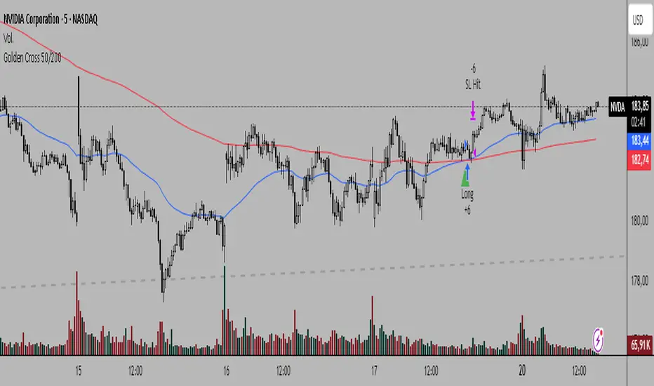
Golden Cross 50/200Simplicity characterizes each of my trading systems and methods. On this occasion, I present a trend-following strategy with simple rules and high profitability.
System Rules:
-Long entries when the 50 EMA crosses above the 200 EMA.
-Stop Loss (SL) placed at the low of 15 candles prior to the entry candle.
-Take Profit (TP) triggered when the 50 EMA crosses below the 200 EMA.
As with any trend-following system, we sacrifice win rate for profitability, and of course, we will focus on traditional markets with a consistent trend-following nature over time.
Recommended Markets and Timeframes:
BTCUSDT H6
August 17, 2017 - October 20, 2025 Total trades: 30
Profitability: +1,682.99%
Win rate: 40%
Outperforms Buy & Hold
BTCUSDT H4
August 17, 2017 - October 20, 2025 Total trades: 42
Profitability: +12,213.49% (high and stable performance curve)
Win rate: 40%
Outperforms Buy & Hold
BTCUSDT H2
August 17, 2017 - October 20, 2025 Total trades: 95
Profitability: +2,363.80%
Win rate: 24.21%
Matches Buy & Hold
BTCUSDT H1
August 17, 2017 - October 20, 2025 Total trades: 203
Profitability: +1,045% (stable performance curve)
Win rate: 25.62%
BTCUSDT 30M
August 17, 2017 - October 20, 2025 Total trades: 393
Profitability: +4,205.51% (high and stable performance curve)
Win rate: 27.74%
Outperforms Buy & Hold
BTCUSDT 15M
August 17, 2017 - October 20, 2025 Total trades: 821
Profitability: +1,311.97%
Win rate: 23.14%
Timeframes such as Daily, 12-hour, 8-hour, and even 5-minute charts are profitable with this system, so feel free to experiment.
Other markets and timeframes to observe include:
-XAUUSD (H1, H4, H6, H8, Daily)
-SPX (Daily: +21,302% profitability since 1871 in 40 trades)
-Tesla (H1, H2, H4, H6, especially M30 and M15)
-Apple (M5, M15, M30, H1, H2, H4…)
-Warner Bros (M5, M15, M30…)
-GOOGL (M5, M15, M30, H1, H2, H4, H6…)
-AMZN (M5, M15, M30, H2, H4, H6…)
-META (M5, M15, M30, H1, H2, H4…)
-NVDA (M5, M15, M30, H1, H2, H4…)
This system not only generates significant profitability but also performs very well in traditional markets, even on lower timeframes like 5-minute charts. In many cases, the returns far exceed Buy & Hold.
I hope this strategy is useful to you. Follow my Spanish-speaking profile if you want to see my market analyses, and send me your good vibes!
Boilerplate Configurable Strategy [Yosiet]This is a Boilerplate Code!
Hello! First of all, let me introduce myself a little bit. I don't come from the world of finance, but from the world of information and communication technologies (ICT) where we specialize in data processing with the aim of automating it and eliminating all human factors and actors in the processes. You could say that I am an algotrader.
That said, in my journey through trading in recent years I have understood that this world is often shown to be incomplete. All those who want to learn about trading only end up learning a small part of what it really entails, they only seek to learn how to read candlesticks. Therefore, I want to share with the entire community a fraction of what I have really understood it to be.
As a computer scientist, the most important thing is the data, it is the raw material of our work and without data you simply cannot do anything. Entropy is simple: Data in -> Data is transformed -> Data out.
The quality of the outgoing data will directly depend on the incoming data, there is no greater mystery or magic in the process. In trading it is no different, because at the end of the day it is nothing more than data. As we often say, if garbage comes in, garbage comes out.
Most people focus on the results only, on the outgoing data, because in the end we all want the same thing, to make easy money. Very few pay attention to the input data, much less to the process.
Now, I am not here to delude you, because there is no bigger lie than easy money, but I am here to give you a boilerplate code that will help you create strategies where you only have to concentrate on the quality of the incoming data.
To the Point
The code is a strategy boilerplate that applies the technique that you decide to customize for the criteria for opening a position. It already has the other factors involved in trading programmed and automated.
1. The Entry
This section of the boilerplate is the one that each individual must customize according to their needs and knowledge. The code is offered with two simple, well-known strategies to exemplify how the code can be reused for your own benefits.
For the purposes of this post on tradingview, I am going to use the simplest of the known strategies in trading for entries: SMA Crossing
// SMA Cross Settings
maFast = ta.sma(close, length)
maSlow = ta.sma(open, length)
The Strategy Properties for all cases published here:
For Stock TSLA H1 From 01/01/2025 To 02/15/2025
For Crypto XMR-USDT 30m From 01/01/2025 To 02/15/2025
For Forex EUR-USD 5m From 01/01/2025 To 02/15/2025
But the goal of this post is not to sell you a dream, else to show you that the same Entry decision works very well for some and does not for others and with this boilerplate code you only have to think of entries, not exits.
2. Schedules, Days, Sessions
As you know, there are an infinite number of markets that are susceptible to the sessions of each country and the news that they announce during those sessions, so the code already offers parameters so that you can condition the days and hours of operation, filter the best time parameters for a specific market and time frame.
3. Data Filtering
The data offered in trading are numerical series presented in vectors on a time axis where an endless number of mathematical equations can be applied to process them, with matrix calculation and non-linear regressions being the best, in my humble opinion.
4. Read Fundamental Macroeconomic Events, News
The boilerplate has integration with the tradingview SDK to detect when news will occur and offers parameters so that you can enable an exclusion time margin to not operate anything during that time window.
5. Direction and Sense
In my experience I have found the peculiarity that the same algorithm works very well for a market in a time frame, but for the same market in another time frame it is only a waste of time and money. So now you can easily decide if you only want to open LONG, SHORT or both side positions and know how effective your strategy really is.
6. Reading the money, THE PURPOSE OF EVERYTHING
The most important section in trading and the reason why many clients usually hire me as a financial programmer, is reading and controlling the money, because in the end everyone wants to win and no one wants to lose. Now they can easily parameterize how the money should flow and this is the genius of this boilerplate, because it is what will really decide if an algorithm (Indicator: A bunch of math equations) for entries will really leave you good money over time.
7. Managing the Risk, The Ego Destroyer
Many trades, little money. Most traders focus on making money and none of them know about statistics and the few who do know something about it, only focus on the winrate. Well, with this code you can unlock what really matters, the true success criteria to be able to live off of trading: Profit Factor, Sortino Ratio, Sharpe Ratio and most importantly, will you really make money?
8. Managing Emotions
Finally, the main reason why many lose money is because they are very bad at managing their emotions, because with this they will no longer need to do so because the boilerplate has already programmed criteria to chase the price in a position, cut losses and maximize profits.
In short, this is a boilerplate code that already has the data processing and data output ready, you only have to worry about the data input.
“And so the trader learned: the greatest edge was not in predicting the storm, but in building a boat that could not sink.”
DISCLAIMER
This post is intended for programmers and quantitative traders who already have a certain level of knowledge and experience. It is not intended to be financial advice or to sell you any money-making script, if you use it, you do so at your own risk.

WASDE DatesOverview
WASDE Dates — a small, focused event indicator that displays confirmed USDA WASDE release dates for 2025 on the chart and marks each release day. The indicator is designed to be a lightweight timing tool for traders who want clean visual reminders and optional alerts around USDA WASDE publications.
Features
• Shows official WASDE release dates for 2025 in a compact chart table.
• Draws on-chart markers and a dotted vertical line on WASDE release days.
• Two alert conditions you can enable in TradingView: "WASDE Day Alert" and "WASDE 24h Reminder".
• Simple table position control (Top/Bottom, Left/Right) in the indicator settings.
• Minimal, self-contained code — no external data feeds or permissions required.
How to use
1. Apply the indicator to any chart and timeframe.
2. Use the indicator settings to choose table position.
3. Enable Alerts (if desired) via TradingView Alerts → choose “WASDE Day Alert” or “WASDE 24h Reminder”.
4. This version contains 2025 confirmed dates only — verify dates for live trading and enable alerts as needed.
Design & rationale
This indicator is intentionally not a technical trading signal. It is an event scheduler focused on clarity and low overhead: combine it with your existing setup to avoid being surprised by WASDE publications and to quickly inspect price action around these event dates.
Limitations & disclaimer
• This script shows **confirmed 2025** WASDE dates only. It does not provide trading advice or entry/exit signals. Use at your own risk.
• Double-check official USDA publishing times before executing trades.
• No external links or contact information are included in this description to comply with TradingView publishing rules.
Feature outlook (V2)
Planned V2 (future release): enhanced countdown (days → hours/minutes), optional inclusion of estimated 2026 dates marked as (TBC), and an invite-only/protected advanced version with reaction overlays (T+1/T+3) and extended alert options. V2 will be announced on this script page when ready.
Changelog
v1 — public release: 2025 confirmed dates, release markers, alerts, table position control.

Dskyz (DAFE) Adaptive Regime - Quant Machine ProDskyz (DAFE) Adaptive Regime - Quant Machine Pro:
Buckle up for the Dskyz (DAFE) Adaptive Regime - Quant Machine Pro, is a strategy that’s your ultimate edge for conquering futures markets like ES, MES, NQ, and MNQ. This isn’t just another script—it’s a quant-grade powerhouse, crafted with precision to adapt to market regimes, deliver multi-factor signals, and protect your capital with futures-tuned risk management. With its shimmering DAFE visuals, dual dashboards, and glowing watermark, it turns your charts into a cyberpunk command center, making trading as thrilling as it is profitable.
Unlike generic scripts clogging up the space, the Adaptive Regime is a DAFE original, built from the ground up to tackle the chaos of futures trading. It identifies market regimes (Trending, Range, Volatile, Quiet) using ADX, Bollinger Bands, and HTF indicators, then fires trades based on a weighted scoring system that blends candlestick patterns, RSI, MACD, and more. Add in dynamic stops, trailing exits, and a 5% drawdown circuit breaker, and you’ve got a system that’s as safe as it is aggressive. Whether you’re a newbie or a prop desk pro, this strat’s your ticket to outsmarting the markets. Let’s break down every detail and see why it’s a must-have.
Why Traders Need This Strategy
Futures markets are a gauntlet—fast moves, volatility spikes (like the April 28, 2025 NQ 1k-point drop), and institutional traps that punish the unprepared. Meanwhile, platforms are flooded with low-effort scripts that recycle old ideas with zero innovation. The Adaptive Regime stands tall, offering:
Adaptive Intelligence: Detects market regimes (Trending, Range, Volatile, Quiet) to optimize signals, unlike one-size-fits-all scripts.
Multi-Factor Precision: Combines candlestick patterns, MA trends, RSI, MACD, volume, and HTF confirmation for high-probability trades.
Futures-Optimized Risk: Calculates position sizes based on $ risk (default: $300), with ATR or fixed stops/TPs tailored for ES/MES.
Bulletproof Safety: 5% daily drawdown circuit breaker and trailing stops keep your account intact, even in chaos.
DAFE Visual Mastery: Pulsing Bollinger Band fills, dynamic SL/TP lines, and dual dashboards (metrics + position) make signals crystal-clear and charts a work of art.
Original Craftsmanship: A DAFE creation, built with community passion, not a rehashed clone of generic code.
Traders need this because it’s a complete, adaptive system that blends quant smarts, user-friendly design, and DAFE flair. It’s your edge to trade with confidence, cut through market noise, and leave the copycats in the dust.
Strategy Components
1. Market Regime Detection
The strategy’s brain is its ability to classify market conditions into five regimes, ensuring signals match the environment.
How It Works:
Trending (Regime 1): ADX > 20, fast/slow EMA spread > 0.3x ATR, HTF RSI > 50 or MACD bullish (htf_trend_bull/bear).
Range (Regime 2): ADX < 25, price range < 3% of close, no HTF trend.
Volatile (Regime 3): BB width > 1.5x avg, ATR > 1.2x avg, HTF RSI overbought/oversold.
Quiet (Regime 4): BB width < 0.8x avg, ATR < 0.9x avg.
Other (Regime 5): Default for unclear conditions.
Indicators: ADX (14), BB width (20), ATR (14, 50-bar SMA), HTF RSI (14, daily default), HTF MACD (12,26,9).
Why It’s Brilliant:
Regime detection adapts signals to market context, boosting win rates in trending or volatile conditions.
HTF RSI/MACD add a big-picture filter, rare in basic scripts.
Visualized via gradient background (green for Trending, orange for Range, red for Volatile, gray for Quiet, navy for Other).
2. Multi-Factor Signal Scoring
Entries are driven by a weighted scoring system that combines candlestick patterns, trend, momentum, and volume for robust signals.
Candlestick Patterns:
Bullish: Engulfing (0.5), hammer (0.4 in Range, 0.2 else), morning star (0.2), piercing (0.2), double bottom (0.3 in Volatile, 0.15 else). Must be near support (low ≤ 1.01x 20-bar low) with volume spike (>1.5x 20-bar avg).
Bearish: Engulfing (0.5), shooting star (0.4 in Range, 0.2 else), evening star (0.2), dark cloud (0.2), double top (0.3 in Volatile, 0.15 else). Must be near resistance (high ≥ 0.99x 20-bar high) with volume spike.
Logic: Patterns are weighted higher in specific regimes (e.g., hammer in Range, double bottom in Volatile).
Additional Factors:
Trend: Fast EMA (20) > slow EMA (50) + 0.5x ATR (trend_bull, +0.2); opposite for trend_bear.
RSI: RSI (14) < 30 (rsi_bull, +0.15); > 70 (rsi_bear, +0.15).
MACD: MACD line > signal (12,26,9, macd_bull, +0.15); opposite for macd_bear.
Volume: ATR > 1.2x 50-bar avg (vol_expansion, +0.1).
HTF Confirmation: HTF RSI < 70 and MACD bullish (htf_bull_confirm, +0.2); RSI > 30 and MACD bearish (htf_bear_confirm, +0.2).
Scoring:
bull_score = sum of bullish factors; bear_score = sum of bearish. Entry requires score ≥ 1.0.
Example: Bullish engulfing (0.5) + trend_bull (0.2) + rsi_bull (0.15) + htf_bull_confirm (0.2) = 1.05, triggers long.
Why It’s Brilliant:
Multi-factor scoring ensures signals are confirmed by multiple market dynamics, reducing false positives.
Regime-specific weights make patterns more relevant (e.g., hammers shine in Range markets).
HTF confirmation aligns with the big picture, a quant edge over simplistic scripts.
3. Futures-Tuned Risk Management
The risk system is built for futures, calculating position sizes based on $ risk and offering flexible stops/TPs.
Position Sizing:
Logic: Risk per trade (default: $300) ÷ (stop distance in points * point value) = contracts, capped at max_contracts (default: 5). Point value = tick value (e.g., $12.5 for ES) * ticks per point (4) * contract multiplier (1 for ES, 0.1 for MES).
Example: $300 risk, 8-point stop, ES ($50/point) → 0.75 contracts, rounded to 1.
Impact: Precise sizing prevents over-leverage, critical for micro contracts like MES.
Stops and Take-Profits:
Fixed: Default stop = 8 points, TP = 16 points (2:1 reward/risk).
ATR-Based: Stop = 1.5x ATR (default), TP = 3x ATR, enabled via use_atr_for_stops.
Logic: Stops set at swing low/high ± stop distance; TPs at 2x stop distance from entry.
Impact: ATR stops adapt to volatility, while fixed stops suit stable markets.
Trailing Stops:
Logic: Activates at 50% of TP distance. Trails at close ± 1.5x ATR (atr_multiplier). Longs: max(trail_stop_long, close - ATR * 1.5); shorts: min(trail_stop_short, close + ATR * 1.5).
Impact: Locks in profits during trends, a game-changer in volatile sessions.
Circuit Breaker:
Logic: Pauses trading if daily drawdown > 5% (daily_drawdown = (max_equity - equity) / max_equity).
Impact: Protects capital during black swan events (e.g., April 27, 2025 ES slippage).
Why It’s Brilliant:
Futures-specific inputs (tick value, multiplier) make it plug-and-play for ES/MES.
Trailing stops and circuit breaker add pro-level safety, rare in off-the-shelf scripts.
Flexible stops (ATR or fixed) suit different trading styles.
4. Trade Entry and Exit Logic
Entries and exits are precise, driven by bull_score/bear_score and protected by drawdown checks.
Entry Conditions:
Long: bull_score ≥ 1.0, no position (position_size <= 0), drawdown < 5% (not pause_trading). Calculates contracts, sets stop at swing low - stop points, TP at 2x stop distance.
Short: bear_score ≥ 1.0, position_size >= 0, drawdown < 5%. Stop at swing high + stop points, TP at 2x stop distance.
Logic: Tracks entry_regime for PNL arrays. Closes opposite positions before entering.
Exit Conditions:
Stop-Loss/Take-Profit: Hits stop or TP (strategy.exit).
Trailing Stop: Activates at 50% TP, trails by ATR * 1.5.
Emergency Exit: Closes if price breaches stop (close < long_stop_price or close > short_stop_price).
Reset: Clears stop/TP prices when flat (position_size = 0).
Why It’s Brilliant:
Score-based entries ensure multi-factor confirmation, filtering out weak signals.
Trailing stops maximize profits in trends, unlike static exits in basic scripts.
Emergency exits add an extra safety layer, critical for futures volatility.
5. DAFE Visuals
The visuals are pure DAFE magic, blending function with cyberpunk flair to make signals intuitive and charts stunning.
Shimmering Bollinger Band Fill:
Display: BB basis (20, white), upper/lower (green/red, 45% transparent). Fill pulses (30–50 alpha) by regime, with glow (60–95 alpha) near bands (close ≥ 0.995x upper or ≤ 1.005x lower).
Purpose: Highlights volatility and key levels with a futuristic glow.
Visuals make complex regimes and signals instantly clear, even for newbies.
Pulsing effects and regime-specific colors add a DAFE signature, setting it apart from generic scripts.
BB glow emphasizes tradeable levels, enhancing decision-making.
Chart Background (Regime Heatmap):
Green — Trending Market: Strong, sustained price movement in one direction. The market is in a trend phase—momentum follows through.
Orange — Range-Bound: Market is consolidating or moving sideways, with no clear up/down trend. Great for mean reversion setups.
Red — Volatile Regime: High volatility, heightened risk, and larger/faster price swings—trade with caution.
Gray — Quiet/Low Volatility: Market is calm and inactive, with small moves—often poor conditions for most strategies.
Navy — Other/Neutral: Regime is uncertain or mixed; signals may be less reliable.
Bollinger Bands Glow (Dynamic Fill):
Neon Red Glow — Warning!: Price is near or breaking above the upper band; momentum is overstretched, watch for overbought conditions or reversals.
Bright Green Glow — Opportunity!: Price is near or breaking below the lower band; market could be oversold, prime for bounce or reversal.
Trend Green Fill — Trending Regime: Fills between bands with green when the market is trending, showing clear momentum.
Gold/Yellow Fill — Range Regime: Fills with gold/aqua in range conditions, showing the market is sideways/oscillating.
Magenta/Red Fill — Volatility Spike: Fills with vivid magenta/red during highly volatile regimes.
Blue Fill — Neutral/Quiet: A soft blue glow for other or uncertain market states.
Moving Averages:
Display: Blue fast EMA (20), red slow EMA (50), 2px.
Purpose: Shows trend direction, with trend_dir requiring ATR-scaled spread.
Dynamic SL/TP Lines:
Display: Pulsing colors (red SL, green TP for Trending; yellow/orange for Range, etc.), 3px, with pulse_alpha for shimmer.
Purpose: Tracks stops/TPs in real-time, color-coded by regime.
6. Dual Dashboards
Two dashboards deliver real-time insights, making the strat a quant command center.
Bottom-Left Metrics Dashboard (2x13):
Metrics: Mode (Active/Paused), trend (Bullish/Bearish/Neutral), ATR, ATR avg, volume spike (YES/NO), RSI (value + Oversold/Overbought/Neutral), HTF RSI, HTF trend, last signal (Buy/Sell/None), regime, bull score.
Display: Black (29% transparent), purple title, color-coded (green for bullish, red for bearish).
Purpose: Consolidates market context and signal strength.
Top-Right Position Dashboard (2x7):
Metrics: Regime, position side (Long/Short/None), position PNL ($), SL, TP, daily PNL ($).
Display: Black (29% transparent), purple title, color-coded (lime for Long, red for Short).
Purpose: Tracks live trades and profitability.
Why It’s Brilliant:
Dual dashboards cover market context and trade status, a rare feature.
Color-coding and concise metrics guide beginners (e.g., green “Buy” = go).
Real-time PNL and SL/TP visibility empower disciplined trading.
7. Performance Tracking
Logic: Arrays (regime_pnl_long/short, regime_win/loss_long/short) track PNL and win/loss by regime (1–5). Updated on trade close (barstate.isconfirmed).
Purpose: Prepares for future adaptive thresholds (e.g., adjust bull_score min based on regime performance).
Why It’s Brilliant: Lays the groundwork for self-optimizing logic, a quant edge over static scripts.
Key Features
Regime-Adaptive: Optimizes signals for Trending, Range, Volatile, Quiet markets.
Futures-Optimized: Precise sizing for ES/MES with tick-based risk inputs.
Multi-Factor Signals: Candlestick patterns, RSI, MACD, and HTF confirmation for robust entries.
Dynamic Exits: ATR/fixed stops, 2:1 TPs, and trailing stops maximize profits.
Safe and Smart: 5% drawdown breaker and emergency exits protect capital.
DAFE Visuals: Shimmering BB fill, pulsing SL/TP, and dual dashboards.
Backtest-Ready: Fixed qty and tick calc for accurate historical testing.
How to Use
Add to Chart: Load on a 5min ES/MES chart in TradingView.
Configure Inputs: Set instrument (ES/MES), tick value ($12.5/$1.25), multiplier (1/0.1), risk ($300 default). Enable ATR stops for volatility.
Monitor Dashboards: Bottom-left for regime/signals, top-right for position/PNL.
Backtest: Run in strategy tester to compare regimes.
Live Trade: Connect to Tradovate or similar. Watch for slippage (e.g., April 27, 2025 ES issues).
Replay Test: Try April 28, 2025 NQ drop to see regime shifts and stops.
Disclaimer
Trading futures involves significant risk of loss and is not suitable for all investors. Past performance does not guarantee future results. Backtest results may differ from live trading due to slippage, fees, or market conditions. Use this strategy at your own risk, and consult a financial advisor before trading. Dskyz (DAFE) Trading Systems is not responsible for any losses incurred.
Backtesting:
Frame: 2023-09-20 - 2025-04-29
Slippage: 3
Fee Typical Range (per side, per contract)
CME Exchange $1.14 – $1.20
Clearing $0.10 – $0.30
NFA Regulatory $0.02
Firm/Broker Commis. $0.25 – $0.80 (retail prop)
TOTAL $1.60 – $2.30 per side
Round Turn: (enter+exit) = $3.20 – $4.60 per contract
Final Notes
The Dskyz (DAFE) Adaptive Regime - Quant Machine Pro is more than a strategy—it’s a revolution. Crafted with DAFE’s signature precision, it rises above generic scripts with adaptive regimes, quant-grade signals, and visuals that make trading a thrill. Whether you’re scalping MES or swinging ES, this system empowers you to navigate markets with confidence and style. Join the DAFE crew, light up your charts, and let’s dominate the futures game!
(This publishing will most likely be taken down do to some miscellaneous rule about properly displaying charting symbols, or whatever. Once I've identified what part of the publishing they want to pick on, I'll adjust and repost.)
Use it with discipline. Use it with clarity. Trade smarter.
**I will continue to release incredible strategies and indicators until I turn this into a brand or until someone offers me a contract.
Created by Dskyz, powered by DAFE Trading Systems. Trade smart, trade bold.
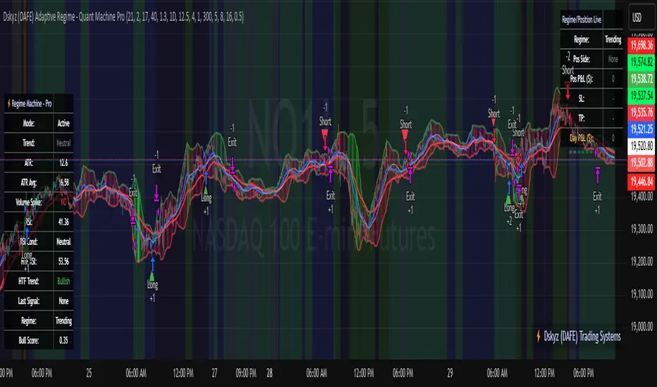
Dskyz (DAFE) Aurora Divergence – Quant Master Dskyz (DAFE) Aurora Divergence – Quant Master
Introducing the Dskyz (DAFE) Aurora Divergence – Quant Master , a strategy that’s your secret weapon for mastering futures markets like MNQ, NQ, MES, and ES. Born from the legendary Aurora Divergence indicator, this fully automated system transforms raw divergence signals into a quant-grade trading machine, blending precision, risk management, and cyberpunk DAFE visuals that make your charts glow like a neon skyline. Crafted with care and driven by community passion, this strategy stands out in a sea of generic scripts, offering traders a unique edge to outsmart institutional traps and navigate volatile markets.
The Aurora Divergence indicator was a cult favorite for spotting price-OBV divergences with its aqua and fuchsia orbs, but traders craved a system to act on those signals with discipline and automation. This strategy delivers, layering advanced filters (z-score, ATR, multi-timeframe, session), dynamic risk controls (kill switches, adaptive stops/TPs), and a real-time dashboard to turn insights into profits. Whether you’re a newbie dipping into futures or a pro hunting reversals, this strat’s got your back with a beginner guide, alerts, and visuals that make trading feel like a sci-fi mission. Let’s dive into every detail and see why this original DAFE creation is a must-have.
Why Traders Need This Strategy
Futures markets are a battlefield—fast-paced, volatile, and riddled with institutional games that can wipe out undisciplined traders. From the April 28, 2025 NQ 1k-point drop to sneaky ES slippage, the stakes are high. Meanwhile, platforms are flooded with unoriginal, low-effort scripts that promise the moon but deliver noise. The Aurora Divergence – Quant Master rises above, offering:
Unmatched Originality: A bespoke system built from the ground up, with custom divergence logic, DAFE visuals, and quant filters that set it apart from copycat clutter.
Automation with Precision: Executes trades on divergence signals, eliminating emotional slip-ups and ensuring consistency, even in chaotic sessions.
Quant-Grade Filters: Z-score, ATR, multi-timeframe, and session checks filter out noise, targeting high-probability reversals.
Robust Risk Management: Daily loss and rolling drawdown kill switches, plus ATR-based stops/TPs, protect your capital like a fortress.
Stunning DAFE Visuals: Aqua/fuchsia orbs, aurora bands, and a glowing dashboard make signals intuitive and charts a work of art.
Community-Driven: Evolved from trader feedback, this strat’s a labor of love, not a recycled knockoff.
Traders need this because it’s a complete, original system that blends accessibility, sophistication, and style. It’s your edge to trade smarter, not harder, in a market full of traps and imitators.
1. Divergence Detection (Core Signal Logic)
The strategy’s core is its ability to detect bullish and bearish divergences between price and On-Balance Volume (OBV), pinpointing reversals with surgical accuracy.
How It Works:
Price Slope: Uses linear regression over a lookback (default: 9 bars) to measure price momentum (priceSlope).
OBV Slope: OBV tracks volume flow (+volume if price rises, -volume if falls), with its slope calculated similarly (obvSlope).
Bullish Divergence: Price slope negative (falling), OBV slope positive (rising), and price above 50-bar SMA (trend_ma).
Bearish Divergence: Price slope positive (rising), OBV slope negative (falling), and price below 50-bar SMA.
Smoothing: Requires two consecutive divergence bars (bullDiv2, bearDiv2) to confirm signals, reducing false positives.
Strength: Divergence intensity (divStrength = |priceSlope * obvSlope| * sensitivity) is normalized (0–1, divStrengthNorm) for visuals.
Why It’s Brilliant:
- Divergences catch hidden momentum shifts, often exploited by institutions, giving you an edge on reversals.
- The 50-bar SMA filter aligns signals with the broader trend, avoiding choppy markets.
- Adjustable lookback (min: 3) and sensitivity (default: 1.0) let you tune for different instruments or timeframes.
2. Filters for Precision
Four advanced filters ensure signals are high-probability and market-aligned, cutting through the noise of volatile futures.
Z-Score Filter:
Logic: Calculates z-score ((close - SMA) / stdev) over a lookback (default: 50 bars). Blocks entries if |z-score| > threshold (default: 1.5) unless disabled (useZFilter = false).
Impact: Avoids trades during extreme price moves (e.g., blow-off tops), keeping you in statistically safe zones.
ATR Percentile Volatility Filter:
Logic: Tracks 14-bar ATR in a 100-bar window (default). Requires current ATR > 80th percentile (percATR) to trade (tradeOk).
Impact: Ensures sufficient volatility for meaningful moves, filtering out low-volume chop.
Multi-Timeframe (HTF) Trend Filter:
Logic: Uses a 50-bar SMA on a higher timeframe (default: 60min). Longs require price > HTF MA (bullTrendOK), shorts < HTF MA (bearTrendOK).
Impact: Aligns trades with the bigger trend, reducing counter-trend losses.
US Session Filter:
Logic: Restricts trading to 9:30am–4:00pm ET (default: enabled, useSession = true) using America/New_York timezone.
Impact: Focuses on high-liquidity hours, avoiding overnight spreads and erratic moves.
Evolution:
- These filters create a robust signal pipeline, ensuring trades are timed for optimal conditions.
- Customizable inputs (e.g., zThreshold, atrPercentile) let traders adapt to their style without compromising quality.
3. Risk Management
The strategy’s risk controls are a masterclass in balancing aggression and safety, protecting capital in volatile markets.
Daily Loss Kill Switch:
Logic: Tracks daily loss (dayStartEquity - strategy.equity). Halts trading if loss ≥ $300 (default) and enabled (killSwitch = true, killSwitchActive).
Impact: Caps daily downside, crucial during events like April 27, 2025 ES slippage.
Rolling Drawdown Kill Switch:
Logic: Monitors drawdown (rollingPeak - strategy.equity) over 100 bars (default). Stops trading if > $1000 (rollingKill).
Impact: Prevents prolonged losing streaks, preserving capital for better setups.
Dynamic Stop-Loss and Take-Profit:
Logic: Stops = entry ± ATR * multiplier (default: 1.0x, stopDist). TPs = entry ± ATR * 1.5x (profitDist). Longs: stop below, TP above; shorts: vice versa.
Impact: Adapts to volatility, keeping stops tight but realistic, with TPs targeting 1.5:1 reward/risk.
Max Bars in Trade:
Logic: Closes trades after 8 bars (default) if not already exited.
Impact: Frees capital from stagnant trades, maintaining efficiency.
Kill Switch Buffer Dashboard:
Logic: Shows smallest buffer ($300 - daily loss or $1000 - rolling DD). Displays 0 (red) if kill switch active, else buffer (green).
Impact: Real-time risk visibility, letting traders adjust dynamically.
Why It’s Brilliant:
- Kill switches and ATR-based exits create a safety net, rare in generic scripts.
- Customizable risk inputs (maxDailyLoss, dynamicStopMult) suit different account sizes.
- Buffer metric empowers disciplined trading, a DAFE signature.
4. Trade Entry and Exit Logic
The entry/exit rules are precise, filtered, and adaptive, ensuring trades are deliberate and profitable.
Entry Conditions:
Long Entry: bullDiv2, cooldown passed (canSignal), ATR filter passed (tradeOk), in US session (inSession), no kill switches (not killSwitchActive, not rollingKill), z-score OK (zOk), HTF trend bullish (bullTrendOK), no existing long (lastDirection != 1, position_size <= 0). Closes shorts first.
Short Entry: Same, but for bearDiv2, bearTrendOK, no long (lastDirection != -1, position_size >= 0). Closes longs first.
Adaptive Cooldown: Default 2 bars (cooldownBars). Doubles (up to 10) after a losing trade, resets after wins (dynamicCooldown).
Exit Conditions:
Stop-Loss/Take-Profit: Set per trade (ATR-based). Exits on stop/TP hits.
Other Exits: Closes if maxBarsInTrade reached, ATR filter fails, or kill switch activates.
Position Management: Ensures no conflicting positions, closing opposites before new entries.
Built To Be Reliable and Consistent:
- Multi-filtered entries minimize false signals, a stark contrast to basic scripts.
- Adaptive cooldown prevents overtrading, especially after losses.
- Clean position handling ensures smooth execution, even in fast markets.
5. DAFE Visuals
The visuals are a DAFE hallmark, blending function with clean flair to make signals intuitive and charts stunning.
Aurora Bands:
Display: Bands around price during divergences (bullish: below low, bearish: above high), sized by ATR * bandwidth (default: 0.5).
Colors: Aqua (bullish), fuchsia (bearish), with transparency tied to divStrengthNorm.
Purpose: Highlights divergence zones with a glowing, futuristic vibe.
Divergence Orbs:
Display: Large/small circles (aqua below for bullish, fuchsia above for bearish) when bullDiv2/bearDiv2 and canSignal. Labels show strength (0–1).
Purpose: Pinpoints entries with eye-catching clarity.
Gradient Background:
Display: Green (bullish), red (bearish), or gray (neutral), 90–95% transparent.
Purpose: Sets the market mood without clutter.
Strategy Plots:
- Stop/TP Lines: Red (stops), green (TPs) for active trades.
- HTF MA: Yellow line for trend context.
- Z-Score: Blue step-line (if enabled).
- Kill Switch Warning: Red background flash when active.
What Makes This Next-Level?:
- Visuals make complex signals (divergences, filters) instantly clear, even for beginners.
- DAFE’s unique aesthetic (orbs, bands) sets it apart from generic scripts, reinforcing originality.
- Functional plots (stops, TPs) enhance trade management.
6. Metrics Dashboard
The top-right dashboard (2x8 table) is your command center, delivering real-time insights.
Metrics:
Daily Loss ($): Current loss vs. day’s start, red if > $300.
Rolling DD ($): Drawdown vs. 100-bar peak, red if > $1000.
ATR Threshold: Current percATR, green if ATR exceeds, red if not.
Z-Score: Current value, green if within threshold, red if not.
Signal: “Bullish Div” (aqua), “Bearish Div” (fuchsia), or “None” (gray).
Action: “Consider Buying”/“Consider Selling” (signal color) or “Wait” (gray).
Kill Switch Buffer ($): Smallest buffer to kill switch, green if > 0, red if 0.
Why This Is Important?:
- Consolidates critical data, making decisions effortless.
- Color-coded metrics guide beginners (e.g., green action = go).
- Buffer metric adds transparency, rare in off-the-shelf scripts.
7. Beginner Guide
Beginner Guide: Middle-right table (shown once on chart load), explains aqua orbs (bullish, buy) and fuchsia orbs (bearish, sell).
Key Features:
Futures-Optimized: Tailored for MNQ, NQ, MES, ES with point-value adjustments.
Highly Customizable: Inputs for lookback, sensitivity, filters, and risk settings.
Real-Time Insights: Dashboard and visuals update every bar.
Backtest-Ready: Fixed qty and tick calc for accurate historical testing.
User-Friendly: Guide, visuals, and dashboard make it accessible yet powerful.
Original Design: DAFE’s unique logic and visuals stand out from generic scripts.
How to Use
Add to Chart: Load on a 5min MNQ/ES chart in TradingView.
Configure Inputs: Adjust instrument, filters, or risk (defaults optimized for MNQ).
Monitor Dashboard: Watch signals, actions, and risk metrics (top-right).
Backtest: Run in strategy tester to evaluate performance.
Live Trade: Connect to a broker (e.g., Tradovate) for automation. Watch for slippage (e.g., April 27, 2025 ES issues).
Replay Test: Use bar replay (e.g., April 28, 2025 NQ drop) to test volatility handling.
Disclaimer
Trading futures involves significant risk of loss and is not suitable for all investors. Past performance is not indicative of future results. Backtest results may not reflect live trading due to slippage, fees, or market conditions. Use this strategy at your own risk, and consult a financial advisor before trading. Dskyz (DAFE) Trading Systems is not responsible for any losses incurred.
Backtesting:
Frame: 2023-09-20 - 2025-04-29
Fee Typical Range (per side, per contract)
CME Exchange $1.14 – $1.20
Clearing $0.10 – $0.30
NFA Regulatory $0.02
Firm/Broker Commis. $0.25 – $0.80 (retail prop)
TOTAL $1.60 – $2.30 per side
Round Turn: (enter+exit) = $3.20 – $4.60 per contract
Final Notes
The Dskyz (DAFE) Aurora Divergence – Quant Master isn’t just a strategy—it’s a movement. Crafted with originality and driven by community passion, it rises above the flood of generic scripts to deliver a system that’s as powerful as it is beautiful. With its quant-grade logic, DAFE visuals, and robust risk controls, it empowers traders to tackle futures with confidence and style. Join the DAFE crew, light up your charts, and let’s outsmart the markets together!
(This publishing will most likely be taken down do to some miscellaneous rule about properly displaying charting symbols, or whatever. Once I've identified what part of the publishing they want to pick on, I'll adjust and repost.)
Use it with discipline. Use it with clarity. Trade smarter.
**I will continue to release incredible strategies and indicators until I turn this into a brand or until someone offers me a contract.
Created by Dskyz, powered by DAFE Trading Systems. Trade fast, trade bold.

Bar Index & TimeLibrary to convert a bar index to a timestamp and vice versa.
Utilizes runtime memory to store the 𝚝𝚒𝚖𝚎 and 𝚝𝚒𝚖𝚎_𝚌𝚕𝚘𝚜𝚎 values of every bar on the chart (and optional future bars), with the ability of storing additional custom values for every chart bar.
█ PREFACE
This library aims to tackle some problems that pine coders (from beginners to advanced) often come across, such as:
I'm trying to draw an object with a 𝚋𝚊𝚛_𝚒𝚗𝚍𝚎𝚡 that is more than 10,000 bars into the past, but this causes my script to fail. How can I convert the 𝚋𝚊𝚛_𝚒𝚗𝚍𝚎𝚡 to a UNIX time so that I can draw visuals using xloc.bar_time ?
I have a diagonal line drawing and I want to get the "y" value at a specific time, but line.get_price() only accepts a bar index value. How can I convert the timestamp into a bar index value so that I can still use this function?
I want to get a previous 𝚘𝚙𝚎𝚗 value that occurred at a specific timestamp. How can I convert the timestamp into a historical offset so that I can use 𝚘𝚙𝚎𝚗 ?
I want to reference a very old value for a variable. How can I access a previous value that is older than the maximum historical buffer size of 𝚟𝚊𝚛𝚒𝚊𝚋𝚕𝚎 ?
This library can solve the above problems (and many more) with the addition of a few lines of code, rather than requiring the coder to refactor their script to accommodate the limitations.
█ OVERVIEW
The core functionality provided is conversion between xloc.bar_index and xloc.bar_time values.
The main component of the library is the 𝙲𝚑𝚊𝚛𝚝𝙳𝚊𝚝𝚊 object, created via the 𝚌𝚘𝚕𝚕𝚎𝚌𝚝𝙲𝚑𝚊𝚛𝚝𝙳𝚊𝚝𝚊() function which basically stores the 𝚝𝚒𝚖𝚎 and 𝚝𝚒𝚖𝚎_𝚌𝚕𝚘𝚜𝚎 of every bar on the chart, and there are 3 more overloads to this function that allow collecting and storing additional data. Once a 𝙲𝚑𝚊𝚛𝚝𝙳𝚊𝚝𝚊 object is created, use any of the exported methods:
Methods to convert a UNIX timestamp into a bar index or bar offset:
𝚝𝚒𝚖𝚎𝚜𝚝𝚊𝚖𝚙𝚃𝚘𝙱𝚊𝚛𝙸𝚗𝚍𝚎𝚡(), 𝚐𝚎𝚝𝙽𝚞𝚖𝚋𝚎𝚛𝙾𝚏𝙱𝚊𝚛𝚜𝙱𝚊𝚌𝚔()
Methods to retrieve the stored data for a bar index:
𝚝𝚒𝚖𝚎𝙰𝚝𝙱𝚊𝚛𝙸𝚗𝚍𝚎𝚡(), 𝚝𝚒𝚖𝚎𝙲𝚕𝚘𝚜𝚎𝙰𝚝𝙱𝚊𝚛𝙸𝚗𝚍𝚎𝚡(), 𝚟𝚊𝚕𝚞𝚎𝙰𝚝𝙱𝚊𝚛𝙸𝚗𝚍𝚎𝚡(), 𝚐𝚎𝚝𝙰𝚕𝚕𝚅𝚊𝚛𝚒𝚊𝚋𝚕𝚎𝚜𝙰𝚝𝙱𝚊𝚛𝙸𝚗𝚍𝚎𝚡()
Methods to retrieve the stored data at a number of bars back (i.e., historical offset):
𝚝𝚒𝚖𝚎(), 𝚝𝚒𝚖𝚎𝙲𝚕𝚘𝚜𝚎(), 𝚟𝚊𝚕𝚞𝚎()
Methods to retrieve all the data points from the earliest bar (or latest bar) stored in memory, which can be useful for debugging purposes:
𝚐𝚎𝚝𝙴𝚊𝚛𝚕𝚒𝚎𝚜𝚝𝚂𝚝𝚘𝚛𝚎𝚍𝙳𝚊𝚝𝚊(), 𝚐𝚎𝚝𝙻𝚊𝚝𝚎𝚜𝚝𝚂𝚝𝚘𝚛𝚎𝚍𝙳𝚊𝚝𝚊()
Note: the library's strong suit is referencing data from very old bars in the past, which is especially useful for scripts that perform its necessary calculations only on the last bar.
█ USAGE
Step 1
Import the library. Replace with the latest available version number for this library.
//@version=6
indicator("Usage")
import n00btraders/ChartData/
Step 2
Create a 𝙲𝚑𝚊𝚛𝚝𝙳𝚊𝚝𝚊 object to collect data on every bar. Do not declare as `var` or `varip`.
chartData = ChartData.collectChartData() // call on every bar to accumulate the necessary data
Step 3
Call any method(s) on the 𝙲𝚑𝚊𝚛𝚝𝙳𝚊𝚝𝚊 object. Do not modify its fields directly.
if barstate.islast
int firstBarTime = chartData.timeAtBarIndex(0)
int lastBarTime = chartData.time(0)
log.info("First `time`: " + str.format_time(firstBarTime) + ", Last `time`: " + str.format_time(lastBarTime))
█ EXAMPLES
• Collect Future Times
The overloaded 𝚌𝚘𝚕𝚕𝚎𝚌𝚝𝙲𝚑𝚊𝚛𝚝𝙳𝚊𝚝𝚊() functions that accept a 𝚋𝚊𝚛𝚜𝙵𝚘𝚛𝚠𝚊𝚛𝚍 argument can additionally store time values for up to 500 bars into the future.
//@version=6
indicator("Example `collectChartData(barsForward)`")
import n00btraders/ChartData/1
chartData = ChartData.collectChartData(barsForward = 500)
var rectangle = box.new(na, na, na, na, xloc = xloc.bar_time, force_overlay = true)
if barstate.islast
int futureTime = chartData.timeAtBarIndex(bar_index + 100)
int lastBarTime = time
box.set_lefttop(rectangle, lastBarTime, open)
box.set_rightbottom(rectangle, futureTime, close)
box.set_text(rectangle, "Extending box 100 bars to the right. Time: " + str.format_time(futureTime))
• Collect Custom Data
The overloaded 𝚌𝚘𝚕𝚕𝚎𝚌𝚝𝙲𝚑𝚊𝚛𝚝𝙳𝚊𝚝𝚊() functions that accept a 𝚟𝚊𝚛𝚒𝚊𝚋𝚕𝚎𝚜 argument can additionally store custom user-specified values for every bar on the chart.
//@version=6
indicator("Example `collectChartData(variables)`")
import n00btraders/ChartData/1
var map variables = map.new()
variables.put("open", open)
variables.put("close", close)
variables.put("open-close midpoint", (open + close) / 2)
variables.put("boolean", open > close ? 1 : 0)
chartData = ChartData.collectChartData(variables = variables)
var fgColor = chart.fg_color
var table1 = table.new(position.top_right, 2, 9, color(na), fgColor, 1, fgColor, 1, true)
var table2 = table.new(position.bottom_right, 2, 9, color(na), fgColor, 1, fgColor, 1, true)
if barstate.isfirst
table.cell(table1, 0, 0, "ChartData.value()", text_color = fgColor)
table.cell(table2, 0, 0, "open ", text_color = fgColor)
table.merge_cells(table1, 0, 0, 1, 0)
table.merge_cells(table2, 0, 0, 1, 0)
for i = 1 to 8
table.cell(table1, 0, i, text_color = fgColor, text_halign = text.align_left, text_font_family = font.family_monospace)
table.cell(table2, 0, i, text_color = fgColor, text_halign = text.align_left, text_font_family = font.family_monospace)
table.cell(table1, 1, i, text_color = fgColor)
table.cell(table2, 1, i, text_color = fgColor)
if barstate.islast
for i = 1 to 8
float open1 = chartData.value("open", 5000 * i)
float open2 = i < 3 ? open : -1
table.cell_set_text(table1, 0, i, "chartData.value(\"open\", " + str.tostring(5000 * i) + "): ")
table.cell_set_text(table2, 0, i, "open : ")
table.cell_set_text(table1, 1, i, str.tostring(open1))
table.cell_set_text(table2, 1, i, open2 >= 0 ? str.tostring(open2) : "Error")
• xloc.bar_index → xloc.bar_time
The 𝚝𝚒𝚖𝚎 value (or 𝚝𝚒𝚖𝚎_𝚌𝚕𝚘𝚜𝚎 value) can be retrieved for any bar index that is stored in memory by the 𝙲𝚑𝚊𝚛𝚝𝙳𝚊𝚝𝚊 object.
//@version=6
indicator("Example `timeAtBarIndex()`")
import n00btraders/ChartData/1
chartData = ChartData.collectChartData()
if barstate.islast
int start = bar_index - 15000
int end = bar_index - 100
// line.new(start, close, end, close) // !ERROR - `start` value is too far from current bar index
start := chartData.timeAtBarIndex(start)
end := chartData.timeAtBarIndex(end)
line.new(start, close, end, close, xloc.bar_time, width = 10)
• xloc.bar_time → xloc.bar_index
Use 𝚝𝚒𝚖𝚎𝚜𝚝𝚊𝚖𝚙𝚃𝚘𝙱𝚊𝚛𝙸𝚗𝚍𝚎𝚡() to find the bar that a timestamp belongs to.
If the timestamp falls in between the close of one bar and the open of the next bar,
the 𝚜𝚗𝚊𝚙 parameter can be used to determine which bar to choose:
𝚂𝚗𝚊𝚙.𝙻𝙴𝙵𝚃 - prefer to choose the leftmost bar (typically used for closing times)
𝚂𝚗𝚊𝚙.𝚁𝙸𝙶𝙷𝚃 - prefer to choose the rightmost bar (typically used for opening times)
𝚂𝚗𝚊𝚙.𝙳𝙴𝙵𝙰𝚄𝙻𝚃 (or 𝚗𝚊) - copies the same behavior as xloc.bar_time uses for drawing objects
//@version=6
indicator("Example `timestampToBarIndex()`")
import n00btraders/ChartData/1
startTimeInput = input.time(timestamp("01 Aug 2025 08:30 -0500"), "Session Start Time")
endTimeInput = input.time(timestamp("01 Aug 2025 15:15 -0500"), "Session End Time")
chartData = ChartData.collectChartData()
if barstate.islastconfirmedhistory
int startBarIndex = chartData.timestampToBarIndex(startTimeInput, ChartData.Snap.RIGHT)
int endBarIndex = chartData.timestampToBarIndex(endTimeInput, ChartData.Snap.LEFT)
line1 = line.new(startBarIndex, 0, startBarIndex, 1, extend = extend.both, color = color.new(color.green, 60), force_overlay = true)
line2 = line.new(endBarIndex, 0, endBarIndex, 1, extend = extend.both, color = color.new(color.green, 60), force_overlay = true)
linefill.new(line1, line2, color.new(color.green, 90))
// using Snap.DEFAULT to show that it is equivalent to drawing lines using `xloc.bar_time` (i.e., it aligns to the same bars)
startBarIndex := chartData.timestampToBarIndex(startTimeInput)
endBarIndex := chartData.timestampToBarIndex(endTimeInput)
line.new(startBarIndex, 0, startBarIndex, 1, extend = extend.both, color = color.yellow, width = 3)
line.new(endBarIndex, 0, endBarIndex, 1, extend = extend.both, color = color.yellow, width = 3)
line.new(startTimeInput, 0, startTimeInput, 1, xloc.bar_time, extend.both, color.new(color.blue, 85), width = 11)
line.new(endTimeInput, 0, endTimeInput, 1, xloc.bar_time, extend.both, color.new(color.blue, 85), width = 11)
• Get Price of Line at Timestamp
The pine script built-in function line.get_price() requires working with bar index values. To get the price of a line in terms of a timestamp, convert the timestamp into a bar index or offset.
//@version=6
indicator("Example `line.get_price()` at timestamp")
import n00btraders/ChartData/1
lineStartInput = input.time(timestamp("01 Aug 2025 08:30 -0500"), "Line Start")
chartData = ChartData.collectChartData()
var diagonal = line.new(na, na, na, na, force_overlay = true)
if time <= lineStartInput
line.set_xy1(diagonal, bar_index, open)
if barstate.islastconfirmedhistory
line.set_xy2(diagonal, bar_index, close)
if barstate.islast
int timeOneWeekAgo = timenow - (7 * timeframe.in_seconds("1D") * 1000)
// Note: could also use `timetampToBarIndex(timeOneWeekAgo, Snap.DEFAULT)` and pass the value directly to `line.get_price()`
int barsOneWeekAgo = chartData.getNumberOfBarsBack(timeOneWeekAgo)
float price = line.get_price(diagonal, bar_index - barsOneWeekAgo)
string formatString = "Time 1 week ago: {0,number,#}\n - Equivalent to {1} bars ago\n\n𝚕𝚒𝚗𝚎.𝚐𝚎𝚝_𝚙𝚛𝚒𝚌𝚎(): {2,number,#.##}"
string labelText = str.format(formatString, timeOneWeekAgo, barsOneWeekAgo, price)
label.new(timeOneWeekAgo, price, labelText, xloc.bar_time, style = label.style_label_lower_right, size = 16, textalign = text.align_left, force_overlay = true)
█ RUNTIME ERROR MESSAGES
This library's functions will generate a custom runtime error message in the following cases:
𝚌𝚘𝚕𝚕𝚎𝚌𝚝𝙲𝚑𝚊𝚛𝚝𝙳𝚊𝚝𝚊() is not called consecutively, or is called more than once on a single bar
Invalid 𝚋𝚊𝚛𝚜𝙵𝚘𝚛𝚠𝚊𝚛𝚍 argument in the 𝚌𝚘𝚕𝚕𝚎𝚌𝚝𝙲𝚑𝚊𝚛𝚝𝙳𝚊𝚝𝚊() function
Invalid 𝚟𝚊𝚛𝚒𝚊𝚋𝚕𝚎𝚜 argument in the 𝚌𝚘𝚕𝚕𝚎𝚌𝚝𝙲𝚑𝚊𝚛𝚝𝙳𝚊𝚝𝚊() function
Invalid 𝚕𝚎𝚗𝚐𝚝𝚑 argument in any of the functions that accept a number of bars back
Note: there is no runtime error generated for an invalid 𝚝𝚒𝚖𝚎𝚜𝚝𝚊𝚖𝚙 or 𝚋𝚊𝚛𝙸𝚗𝚍𝚎𝚡 argument in any of the functions. Instead, the functions will assign 𝚗𝚊 to the returned values.
Any other runtime errors are due to incorrect usage of the library.
█ NOTES
• Function Descriptions
The library source code uses Markdown for the exported functions. Hover over a function/method call in the Pine Editor to display formatted, detailed information about the function/method.
//@version=6
indicator("Demo Function Tooltip")
import n00btraders/ChartData/1
chartData = ChartData.collectChartData()
int barIndex = chartData.timestampToBarIndex(timenow)
log.info(str.tostring(barIndex))
• Historical vs. Realtime Behavior
Under the hood, the data collector for this library is declared as `var`. Because of this, the 𝙲𝚑𝚊𝚛𝚝𝙳𝚊𝚝𝚊 object will always reflect the latest available data on realtime updates. Any data that is recorded for historical bars will remain unchanged throughout the execution of a script.
//@version=6
indicator("Demo Realtime Behavior")
import n00btraders/ChartData/1
var map variables = map.new()
variables.put("open", open)
variables.put("close", close)
chartData = ChartData.collectChartData(variables)
if barstate.isrealtime
varip float initialOpen = open
varip float initialClose = close
varip int updateCount = 0
updateCount += 1
float latestOpen = open
float latestClose = close
float recordedOpen = chartData.valueAtBarIndex("open", bar_index)
float recordedClose = chartData.valueAtBarIndex("close", bar_index)
string formatString = "# of updates: {0}\n\n𝚘𝚙𝚎𝚗 at update #1: {1,number,#.##}\n𝚌𝚕𝚘𝚜𝚎 at update #1: {2,number,#.##}\n\n"
+ "𝚘𝚙𝚎𝚗 at update #{0}: {3,number,#.##}\n𝚌𝚕𝚘𝚜𝚎 at update #{0}: {4,number,#.##}\n\n"
+ "𝚘𝚙𝚎𝚗 stored in memory: {5,number,#.##}\n𝚌𝚕𝚘𝚜𝚎 stored in memory: {6,number,#.##}"
string labelText = str.format(formatString, updateCount, initialOpen, initialClose, latestOpen, latestClose, recordedOpen, recordedClose)
label.new(bar_index, close, labelText, style = label.style_label_left, force_overlay = true)
• Collecting Chart Data for Other Contexts
If your use case requires collecting chart data from another context, avoid directly retrieving the 𝙲𝚑𝚊𝚛𝚝𝙳𝚊𝚝𝚊 object as this may exceed memory limits .
//@version=6
indicator("Demo Return Calculated Results")
import n00btraders/ChartData/1
timeInput = input.time(timestamp("01 Sep 2025 08:30 -0500"), "Time")
var int oneMinuteBarsAgo = na
// !ERROR - Memory Limits Exceeded
// chartDataArray = request.security_lower_tf(syminfo.tickerid, "1", ChartData.collectChartData())
// oneMinuteBarsAgo := chartDataArray.last().getNumberOfBarsBack(timeInput)
// function that returns calculated results (a single integer value instead of an entire `ChartData` object)
getNumberOfBarsBack() =>
chartData = ChartData.collectChartData()
chartData.getNumberOfBarsBack(timeInput)
calculatedResultsArray = request.security_lower_tf(syminfo.tickerid, "1", getNumberOfBarsBack())
oneMinuteBarsAgo := calculatedResultsArray.size() > 0 ? calculatedResultsArray.last() : na
if barstate.islast
string labelText = str.format("The selected timestamp occurs 1-minute bars ago", oneMinuteBarsAgo)
label.new(bar_index, hl2, labelText, style = label.style_label_left, size = 16, force_overlay = true)
• Memory Usage
The library's convenience and ease of use comes at the cost of increased usage of computational resources. For simple scripts, using this library will likely not cause any issues with exceeding memory limits. But for large and complex scripts, you can reduce memory issues by specifying a lower 𝚌𝚊𝚕𝚌_𝚋𝚊𝚛𝚜_𝚌𝚘𝚞𝚗𝚝 amount in the indicator() or strategy() declaration statement.
//@version=6
// !ERROR - Memory Limits Exceeded using the default number of bars available (~20,000 bars for Premium plans)
//indicator("Demo `calc_bars_count` parameter")
// Reduce number of bars using `calc_bars_count` parameter
indicator("Demo `calc_bars_count` parameter", calc_bars_count = 15000)
import n00btraders/ChartData/1
map variables = map.new()
variables.put("open", open)
variables.put("close", close)
variables.put("weekofyear", weekofyear)
variables.put("dayofmonth", dayofmonth)
variables.put("hour", hour)
variables.put("minute", minute)
variables.put("second", second)
// simulate large memory usage
chartData0 = ChartData.collectChartData(variables)
chartData1 = ChartData.collectChartData(variables)
chartData2 = ChartData.collectChartData(variables)
chartData3 = ChartData.collectChartData(variables)
chartData4 = ChartData.collectChartData(variables)
chartData5 = ChartData.collectChartData(variables)
chartData6 = ChartData.collectChartData(variables)
chartData7 = ChartData.collectChartData(variables)
chartData8 = ChartData.collectChartData(variables)
chartData9 = ChartData.collectChartData(variables)
log.info(str.tostring(chartData0.time(0)))
log.info(str.tostring(chartData1.time(0)))
log.info(str.tostring(chartData2.time(0)))
log.info(str.tostring(chartData3.time(0)))
log.info(str.tostring(chartData4.time(0)))
log.info(str.tostring(chartData5.time(0)))
log.info(str.tostring(chartData6.time(0)))
log.info(str.tostring(chartData7.time(0)))
log.info(str.tostring(chartData8.time(0)))
log.info(str.tostring(chartData9.time(0)))
if barstate.islast
result = table.new(position.middle_right, 1, 1, force_overlay = true)
table.cell(result, 0, 0, "Script Execution Successful ✅", text_size = 40)
█ EXPORTED ENUMS
Snap
Behavior for determining the bar that a timestamp belongs to.
Fields:
LEFT : Snap to the leftmost bar.
RIGHT : Snap to the rightmost bar.
DEFAULT : Default `xloc.bar_time` behavior.
Note: this enum is used for the 𝚜𝚗𝚊𝚙 parameter of 𝚝𝚒𝚖𝚎𝚜𝚝𝚊𝚖𝚙𝚃𝚘𝙱𝚊𝚛𝙸𝚗𝚍𝚎𝚡().
█ EXPORTED TYPES
Note: users of the library do not need to worry about directly accessing the fields of these types; all computations are done through method calls on an object of the 𝙲𝚑𝚊𝚛𝚝𝙳𝚊𝚝𝚊 type.
Variable
Represents a user-specified variable that can be tracked on every chart bar.
Fields:
name (series string) : Unique identifier for the variable.
values (array) : The array of stored values (one value per chart bar).
ChartData
Represents data for all bars on a chart.
Fields:
bars (series int) : Current number of bars on the chart.
timeValues (array) : The `time` values of all chart (and future) bars.
timeCloseValues (array) : The `time_close` values of all chart (and future) bars.
variables (array) : Additional custom values to track on all chart bars.
█ EXPORTED FUNCTIONS
collectChartData()
Collects and tracks the `time` and `time_close` value of every bar on the chart.
Returns: `ChartData` object to convert between `xloc.bar_index` and `xloc.bar_time`.
collectChartData(barsForward)
Collects and tracks the `time` and `time_close` value of every bar on the chart as well as a specified number of future bars.
Parameters:
barsForward (simple int) : Number of future bars to collect data for.
Returns: `ChartData` object to convert between `xloc.bar_index` and `xloc.bar_time`.
collectChartData(variables)
Collects and tracks the `time` and `time_close` value of every bar on the chart. Additionally, tracks a custom set of variables for every chart bar.
Parameters:
variables (simple map) : Custom values to collect on every chart bar.
Returns: `ChartData` object to convert between `xloc.bar_index` and `xloc.bar_time`.
collectChartData(barsForward, variables)
Collects and tracks the `time` and `time_close` value of every bar on the chart as well as a specified number of future bars. Additionally, tracks a custom set of variables for every chart bar.
Parameters:
barsForward (simple int) : Number of future bars to collect data for.
variables (simple map) : Custom values to collect on every chart bar.
Returns: `ChartData` object to convert between `xloc.bar_index` and `xloc.bar_time`.
█ EXPORTED METHODS
method timestampToBarIndex(chartData, timestamp, snap)
Converts a UNIX timestamp to a bar index.
Namespace types: ChartData
Parameters:
chartData (series ChartData) : The `ChartData` object.
timestamp (series int) : A UNIX time.
snap (series Snap) : A `Snap` enum value.
Returns: A bar index, or `na` if unable to find the appropriate bar index.
method getNumberOfBarsBack(chartData, timestamp)
Converts a UNIX timestamp to a history-referencing length (i.e., number of bars back).
Namespace types: ChartData
Parameters:
chartData (series ChartData) : The `ChartData` object.
timestamp (series int) : A UNIX time.
Returns: A bar offset, or `na` if unable to find a valid number of bars back.
method timeAtBarIndex(chartData, barIndex)
Retrieves the `time` value for the specified bar index.
Namespace types: ChartData
Parameters:
chartData (series ChartData) : The `ChartData` object.
barIndex (int) : The bar index.
Returns: The `time` value, or `na` if there is no `time` stored for the bar index.
method time(chartData, length)
Retrieves the `time` value of the bar that is `length` bars back relative to the latest bar.
Namespace types: ChartData
Parameters:
chartData (series ChartData) : The `ChartData` object.
length (series int) : Number of bars back.
Returns: The `time` value `length` bars ago, or `na` if there is no `time` stored for that bar.
method timeCloseAtBarIndex(chartData, barIndex)
Retrieves the `time_close` value for the specified bar index.
Namespace types: ChartData
Parameters:
chartData (series ChartData) : The `ChartData` object.
barIndex (series int) : The bar index.
Returns: The `time_close` value, or `na` if there is no `time_close` stored for the bar index.
method timeClose(chartData, length)
Retrieves the `time_close` value of the bar that is `length` bars back from the latest bar.
Namespace types: ChartData
Parameters:
chartData (series ChartData) : The `ChartData` object.
length (series int) : Number of bars back.
Returns: The `time_close` value `length` bars ago, or `na` if there is none stored.
method valueAtBarIndex(chartData, name, barIndex)
Retrieves the value of a custom variable for the specified bar index.
Namespace types: ChartData
Parameters:
chartData (series ChartData) : The `ChartData` object.
name (series string) : The variable name.
barIndex (series int) : The bar index.
Returns: The value of the variable, or `na` if that variable is not stored for the bar index.
method value(chartData, name, length)
Retrieves a variable value of the bar that is `length` bars back relative to the latest bar.
Namespace types: ChartData
Parameters:
chartData (series ChartData) : The `ChartData` object.
name (series string) : The variable name.
length (series int) : Number of bars back.
Returns: The value `length` bars ago, or `na` if that variable is not stored for the bar index.
method getAllVariablesAtBarIndex(chartData, barIndex)
Retrieves all custom variables for the specified bar index.
Namespace types: ChartData
Parameters:
chartData (series ChartData) : The `ChartData` object.
barIndex (series int) : The bar index.
Returns: Map of all custom variables that are stored for the specified bar index.
method getEarliestStoredData(chartData)
Gets all values from the earliest bar data that is currently stored in memory.
Namespace types: ChartData
Parameters:
chartData (series ChartData) : The `ChartData` object.
Returns: A tuple:
method getLatestStoredData(chartData, futureData)
Gets all values from the latest bar data that is currently stored in memory.
Namespace types: ChartData
Parameters:
chartData (series ChartData) : The `ChartData` object.
futureData (series bool) : Whether to include the future data that is stored in memory.
Returns: A tuple:

FNGAdataCloseClose prices for FNGA ETF (Dec 2018–May 2025)
The Close prices for FNGA ETF (December 2018 – May 2025) represent the final trading price recorded at the end of each regular U.S. market session (4:00 p.m. Eastern Time) over the entire lifespan of this leveraged exchange-traded note. Initially issued under the ticker FNGU and later rebranded as FNGA in March 2025 before its redemption in May 2025, the product was designed to provide 3x daily leveraged exposure to the MicroSectors FANG+™ Index, which tracks a concentrated group of large-cap technology and tech-enabled growth leaders such as Apple, Amazon, Meta (Facebook), Netflix, and Alphabet (Google).
Close prices are widely regarded as the most important reference point in market data because they establish the official end-of-day valuation of a security. For leveraged products like FNGA, the closing price is especially critical, since it directly determines the reset value for the following trading session. This daily compounding effect means that FNGA’s closing levels often diverged significantly from the long-term performance of its underlying index, creating both opportunities and risks for traders.

FNGAdataHighHigh prices for FNGA ETF (Dec 2018–May 2025)
The High prices for FNGA ETF (December 2018 – May 2025) represent the maximum trading price reached during each regular U.S. market session over the entire trading lifespan of this leveraged exchange-traded note. Originally issued under the ticker FNGU, and later rebranded as FNGA in March 2025 before its redemption, the fund was designed to deliver 3x daily leveraged exposure to the MicroSectors FANG+™ Index. This index focused on a concentrated group of large-cap technology and technology-enabled companies such as Facebook (Meta), Amazon, Apple, Netflix, and Google (Alphabet), along with a few other growth leaders.
The High price data from December 2018 through May 2025 is crucial for understanding how FNGA behaved during intraday trading sessions. Because FNGA was a daily resetting 3x leveraged product, its intraday highs often displayed extreme sensitivity to movements in the underlying FANG+™ stocks, resulting in sharp upward spikes during bullish days and pronounced volatility during broader market rallies.

Dskyz (DAFE) Quantum Sentiment Flux - Beginners Dskyz (DAFE) Quantum Sentiment Flux - Beginners:
Welcome to the Dskyz (DAFE) Quantum Sentiment Flux - Beginners , a strategy and concept that’s your ultimate wingman for trading futures like MNQ, NQ, MES, and ES. This gem combines lightning-fast momentum signals, market sentiment smarts, and bulletproof risk management into a system so intuitive, even newbies can trade like pros. With clean DAFE visuals, preset modes for every vibe, and a revamped dashboard that’s basically a market GPS, this strategy makes futures trading feel like a high-octane sci-fi mission.
Built on the Dskyz (DAFE) legacy of Aurora Divergence, the Quantum Sentiment Flux is designed to empower beginners while giving seasoned traders a lean, sentiment-driven edge. It uses fast/slow EMA crossovers for entries, filters trades with VIX, SPX trends, and sector breadth, and keeps your account safe with adaptive stops and cooldowns. Tuned for more action with faster signals and a slick bottom-left dashboard, this updated version is ready to light up your charts and outsmart institutional traps. Let’s dive into why this strat’s a must-have and break down its brilliance.
Why Traders Need This Strategy
Futures markets are a wild ride—fast moves, volatility spikes (like the April 28, 2025 NQ 1k-point drop), and institutional games that can wreck unprepared traders. Beginners often get lost in complex systems or burned by impulsive trades. The Quantum Sentiment Flux is the antidote, offering:
Dead-Simple Setup: Preset modes (Aggressive, Balanced, Conservative) auto-tune signals, risk, and sizing, so you can trade without a quant degree.
Sentiment Superpower: VIX filter, SPX trend, and sector breadth visuals keep you aligned with market health, dodging chop and riding trends.
Ironclad Safety: Tighter ATR-based stops, 2:1 take-profits, and preset cooldowns protect your capital, even in chaotic sessions.
Next-Level Visuals: Green/red entry triangles, vibrant EMAs, a sector breadth background, and a beefed-up dashboard make signals and context pop.
DAFE Swagger: The clean aesthetics, sleek dashboard—ties it to Dskyz’s elite brand, making your charts a work of art.
Traders need this because it’s a plug-and-play system that blends beginner-friendly simplicity with pro-level market awareness. Whether you’re just starting or scalping 5min MNQ, this strat’s your key to trading with confidence and style.
Strategy Components
1. Core Signal Logic (High-Speed Momentum)
The strategy’s engine is a momentum-based system using fast and slow Exponential Moving Averages (EMAs), now tuned for faster, more frequent trades.
How It Works:
Fast/Slow EMAs: Fast EMA (Aggressive: 5, Balanced: 7, Conservative: 9 bars) and slow EMA (12/14/18 bars) track short-term vs. longer-term momentum.
Crossover Signals:
Buy: Fast EMA crosses above slow EMA, and trend_dir = 1 (fast EMA > slow EMA + ATR * strength threshold).
Sell: Fast EMA crosses below slow EMA, and trend_dir = -1 (fast EMA < slow EMA - ATR * strength threshold).
Strength Filter: ma_strength = fast EMA - slow EMA must exceed an ATR-scaled threshold (Aggressive: 0.15, Balanced: 0.18, Conservative: 0.25) for robust signals.
Trend Direction: trend_dir confirms momentum, filtering out weak crossovers in choppy markets.
Evolution:
Faster EMAs (down from 7–10/21–50) catch short-term trends, perfect for active futures markets.
Lower strength thresholds (0.15–0.25 vs. 0.3–0.5) make signals more sensitive, boosting trade frequency without sacrificing quality.
Preset tuning ensures beginners get optimized settings, while pros can tweak via mode selection.
2. Market Sentiment Filters
The strategy leans hard into market sentiment with a VIX filter, SPX trend analysis, and sector breadth visuals, keeping trades aligned with the big picture.
VIX Filter:
Logic: Blocks long entries if VIX > threshold (default: 20, can_long = vix_close < vix_limit). Shorts are always allowed (can_short = true).
Impact: Prevents longs during high-fear markets (e.g., VIX spikes in crashes), while allowing shorts to capitalize on downturns.
SPX Trend Filter:
Logic: Compares S&P 500 (SPX) close to its SMA (Aggressive: 5, Balanced: 8, Conservative: 12 bars). spx_trend = 1 (UP) if close > SMA, -1 (DOWN) if < SMA, 0 (FLAT) if neutral.
Impact: Provides dashboard context, encouraging trades that align with market direction (e.g., longs in UP trend).
Sector Breadth (Visual):
Logic: Tracks 10 sector ETFs (XLK, XLF, XLE, etc.) vs. their SMAs (same lengths as SPX). Each sector scores +1 (bullish), -1 (bearish), or 0 (neutral), summed as breadth (-10 to +10).
Display: Green background if breadth > 4, red if breadth < -4, else neutral. Dashboard shows sector trends (↑/↓/-).
Impact: Faster SMA lengths make breadth more responsive, reflecting sector rotations (e.g., tech surging, energy lagging).
Why It’s Brilliant:
- VIX filter adds pro-level volatility awareness, saving beginners from panic-driven losses.
- SPX and sector breadth give a 360° view of market health, boosting signal confidence (e.g., green BG + buy signal = high-probability trade).
- Shorter SMAs make sentiment visuals react faster, perfect for 5min charts.
3. Risk Management
The risk controls are a fortress, now tighter and more dynamic to support frequent trading while keeping accounts safe.
Preset-Based Risk:
Aggressive: Fast EMAs (5/12), tight stops (1.1x ATR), 1-bar cooldown. High trade frequency, higher risk.
Balanced: EMAs (7/14), 1.2x ATR stops, 1-bar cooldown. Versatile for most traders.
Conservative: EMAs (9/18), 1.3x ATR stops, 2-bar cooldown. Safer, fewer trades.
Impact: Auto-scales risk to match style, making it foolproof for beginners.
Adaptive Stops and Take-Profits:
Logic: Stops = entry ± ATR * atr_mult (1.1–1.3x, down from 1.2–2.0x). Take-profits = entry ± ATR * take_mult (2x stop distance, 2:1 reward/risk). Longs: stop below entry, TP above; shorts: vice versa.
Impact: Tighter stops increase trade turnover while maintaining solid risk/reward, adapting to volatility.
Trade Cooldown:
Logic: Preset-driven (Aggressive/Balanced: 1 bar, Conservative: 2 bars vs. old user-input 2). Ensures bar_index - last_trade_bar >= cooldown.
Impact: Faster cooldowns (especially Aggressive/Balanced) allow more trades, balanced by VIX and strength filters.
Contract Sizing:
Logic: User sets contracts (default: 1, max: 10), no preset cap (unlike old 7/5/3 suggestion).
Impact: Flexible but risks over-leverage; beginners should stick to low contracts.
Built To Be Reliable and Consistent:
- Tighter stops and faster cooldowns make it a high-octane system without blowing up accounts.
- Preset-driven risk removes guesswork, letting newbies trade confidently.
- 2:1 TPs ensure profitable trades outweigh losses, even in volatile sessions like April 27, 2025 ES slippage.
4. Trade Entry and Exit Logic
The entry/exit rules are simple yet razor-sharp, now with VIX filtering and faster signals:
Entry Conditions:
Long Entry: buy_signal (fast EMA crosses above slow EMA, trend_dir = 1), no position (strategy.position_size = 0), cooldown passed (can_trade), and VIX < 20 (can_long). Enters with user-defined contracts.
Short Entry: sell_signal (fast EMA crosses below slow EMA, trend_dir = -1), no position, cooldown passed, can_short (always true).
Logic: Tracks last_entry_bar for visuals, last_trade_bar for cooldowns.
Exit Conditions:
Stop-Loss/Take-Profit: ATR-based stops (1.1–1.3x) and TPs (2x stop distance). Longs exit if price hits stop (below) or TP (above); shorts vice versa.
No Other Exits: Keeps it straightforward, relying on stops/TPs.
5. DAFE Visuals
The visuals are pure DAFE magic, blending clean function with informative metrics utilized by professionals, now enhanced by faster signals and a responsive breadth background:
EMA Plots:
Display: Fast EMA (blue, 2px), slow EMA (orange, 2px), using faster lengths (5–9/12–18).
Purpose: Highlights momentum shifts, with crossovers signaling entries.
Sector Breadth Background:
Display: Green (90% transparent) if breadth > 4, red (90%) if breadth < -4, else neutral.
Purpose: Faster breadth_sma_len (5–12 vs. 10–50) reflects sector shifts in real-time, reinforcing signal strength.
- Visuals are intuitive, turning complex signals into clear buy/sell cues.
- Faster breadth background reacts to market rotations (e.g., tech vs. energy), giving a pro-level edge.
6. Sector Breadth Dashboard
The new bottom-left dashboard is a game-changer, a 3x16 table (black/gray theme) that’s your market command center:
Metrics:
VIX: Current VIX (red if > 20, gray if not).
SPX: Trend as “UP” (green), “DOWN” (red), or “FLAT” (gray).
Trade Longs: “OK” (green) if VIX < 20, “BLOCK” (red) if not.
Sector Breadth: 10 sectors (Tech, Financial, etc.) with trend arrows (↑ green, ↓ red, - gray).
Placeholder Row: Empty for future metrics (e.g., ATR, breadth score).
Purpose: Consolidates regime, volatility, market trend, and sector data, making decisions a breeze.
- VIX and SPX metrics add context, helping beginners avoid bad trades (e.g., no longs if “BLOCK”).
Sector arrows show market health at a glance, like a cheat code for sentiment.
Key Features
Beginner-Ready: Preset modes and clear visuals make futures trading a breeze.
Sentiment-Driven: VIX filter, SPX trend, and sector breadth keep you in sync with the market.
High-Frequency: Faster EMAs, tighter stops, and short cooldowns boost trade volume.
Safe and Smart: Adaptive stops/TPs and cooldowns protect capital while maximizing wins.
Visual Mastery: DAFE’s clean flair, EMAs, dashboard—makes trading fun and clear.
Backtestable: Lean code and fixed qty ensure accurate historical testing.
How to Use
Add to Chart: Load on a 5min MNQ/ES chart in TradingView.
Pick Preset: Aggressive (scalping), Balanced (versatile), or Conservative (safe). Balanced is default.
Set Contracts: Default 1, max 10. Stick low for safety.
Check Dashboard: Bottom-left shows preset, VIX, SPX, and sectors. “OK” + green breadth = strong buy.
Backtest: Run in strategy tester to compare modes.
Live Trade: Connect to Tradovate or similar. Watch for slippage (e.g., April 27, 2025 ES issues).
Replay Test: Try April 28, 2025 NQ drop to see VIX filter and stops in action.
Why It’s Brilliant
The Dskyz (DAFE) Quantum Sentiment Flux - Beginners is a masterpiece of simplicity and power. It takes pro-level tools—momentum, VIX, sector breadth—and wraps them in a system anyone can run. Faster signals and tighter stops make it a trading machine, while the VIX filter and dashboard keep you ahead of market chaos. The DAFE visuals and bottom-left command center turn your chart into a futuristic cockpit, guiding you through every trade. For beginners, it’s a safe entry to futures; for pros, it’s a scalping beast with sentiment smarts. This strat doesn’t just trade—it transforms how you see the market.
Final Notes
This is more than a strategy—it’s your launchpad to mastering futures with Dskyz (DAFE) flair. The Quantum Sentiment Flux blends accessibility, speed, and market savvy to help you outsmart the game. Load it, watch those triangles glow, and let’s make the markets your canvas!
Official Statement from Pine Script Team
(see TradingView help docs and forums):
"This warning may appear when you call functions such as ta.sma inside a request.security in a loop. There is no runtime impact. If you need to loop through a dynamic list of tickers, this cannot be avoided in the present version... Values will still be correct. Ignore this warning in such contexts."
(This publishing will most likely be taken down do to some miscellaneous rule about properly displaying charting symbols, or whatever. Once I've identified what part of the publishing they want to pick on, I'll adjust and repost.)
Use it with discipline. Use it with clarity. Trade smarter.
**I will continue to release incredible strategies and indicators until I turn this into a brand or until someone offers me a contract.
Created by Dskyz, powered by DAFE Trading Systems. Trade fast, trade bold.