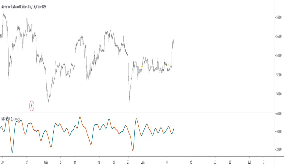
RSI Stochastic AlignmentRSI Stochastic Alignment input RSI and Stochastic into 1 windows and align them to find bullish and bearish divergence.
A. The Line display in windows:
1. Fast RSI (green line) is RSI(close,3)
2. Slow Rsi (red line) is Linear Regession of Fast RSI with 5 period and offset 0 = linreg(rsi,5,0)
3. Fast Stochastic (blue line) is %K of Stochastic
4. Slow Stochastic (aqua line) is %D of Stochastic
B. Alignment and Divergence Detect
1. Bearish Divergence:
* Slow RSI at top
* Fast Stochastic at bottom
* Fast RSI over overbought level (default = 70)
* Slow Stochastic under overbought level minus a constant value (Divergence Power value, default this value = 1)
2. Bullish Divergence:
* Fast Stochastic at top
* Slow RSI at bottom
* Fast RSI under oversold level (default = 30)
* Slow Stochastic over oversold level plus a constant value (Divergence Power value, default this value = 1)
C. Script Option
1. RSI value adjustable
2. Stochastic value adjustable
3. Overbought and Oversold Level adjustable
4. Enable/Disable Level line
5. Enable/Disable Divergence Column
6. Enable/Disable Key Bar Colored
"如何用wind搜索股票的发行价和份数" için komut dosyalarını ara

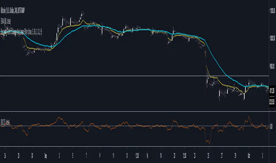
Narrow Bandpass FilterIn technical analysis most bandpass filters like the MACD, TRIX, AO, or COG will have a non-symmetrical frequency response, in fact, this one is generally right-skewed. As such these oscillators will not fully remove lower and higher frequency components from the input signal, the following indicator is a bandpass filter with a more symmetrical frequency response with the possibility to have a narrow bandwidth, this allows the indicator to potentially isolate sinusoids from the input signal.
Indicator & Settings
The filter is calculated via convolution, if we take into account that the frequency response of a filter is the Fourier transform of its weighting function we can deduce that we can get a narrow response by using a sinusoid sin(2𝛑nf) as the weighting function, with the peak of the frequency response being equal to f , this makes the filter quite easy to control by the user, as this one can choose the frequency to be isolated. The length of the weighting function controls the bandwidth of the frequency response, with a higher length returning an ever-smaller frequency response width.
In the indicator settings the "Cycle Period" determine the period of the sinusoid used as a weighting function, while "Bandwidth" determine the filter passband width, with higher values returning a narrower passband, this setting also determine the length of the convolution, because the sum of the weights must add to 0 we know that the length of the convolution must be a multiple of "Cycle Period", so the length of the convolution is equal to "Cycle Period × Bandwidth".
Finally, the windowing option determines if a window is applied to the weighting function, a weighting function allow to remove ripples in the filter frequency response
Above both indicators have a Cycle period of 100 and a Bandwidth of 4, we can see that the indicator with no windowing don't fully remove the trend component in the price, this is due to the presence of ripples allowing lower frequency components to pass, this is not the case for the windowed version.
In theory, an ultra-narrow passband would allow to fully isolate pure sinusoids, below the cycle period of interest is 20
using a bandwidth equal to 10 allow to retain that sinusoid, however, note that this sinusoid is subject to phase shift and that it might not be a dominant frequency in the price.
Decaying Rate of Change Non Linear FilterThis is a potential solution to dealing with the inherent lag in most filters especially with instruments such as BTC and the effects of long periods of low volatility followed by massive volatility spikes as well as whipsaws/barts etc.
We can try and solve these issues in a number of ways, adaptive lengths, dynamic weighting etc. This filter uses a non linear weighting combined with an exponential decay rate.
With the non linear weighting the filter can become very responsive to sudden volatility spikes. We can use a short length absolute rate of change as a method to improve weighting of relative high volatility.
c1 = abs(close - close ) / close
Which gives us a fairly simple filter :
filter = sum(c1 * close,periods) / sum(c1,periods)
At this point if we want to control the relative magnitude of the ROC coefficients we can do so by raising it to a power.
c2 = pow(c1, x)
Where x approaches zero the coefficient approaches 1 or a linear filter. At x = 1 we have an unmodified coefficient and higher values increase the relative magnitude of the response. As an extreme example with x = 10 we effectively isolate the highest ROC candle within the window (which has some novel support resistance horizontals as those closes are often important). This controls the degree of responsiveness, so we can magnify the responsiveness, but with the trade off of overshoot/persistence.
So now we have the problem whereby that a highly weighted data point from a high volatility event persists within the filter window. And to a possibly extreme degree, if a reversal occurs we get a potentially large "overshoot" and in a way actually induced a large amount of lag for future price action.
This filter compensates for this effect by exponentially decaying the abs(ROC) coefficient over time, so as a high volatility event passes through the filter window it receives exponentially less weighting allowing more recent prices to receive a higher relative weighting than they would have.
c3 = c2 * pow(1 - percent_decay, periods_back)
This is somewhat similar to an EMA, however with an EMA being recursive that event will persist forever (to some degree) in the calculation. Here we are using a fixed window, so once the event is behind the window it's completely removed from the calculation
I've added Ehler's Super Smoother as an optional smoothing function as some highly non linear settings benefit from smoothing. I can't remember where I got the original SS code snippet, so if you recognize it as yours msg me and I'll link you here.
ORB Strategy: Extensions & Custom SL (EOD & Live Lines)That's a great request. Since you've now built a complex Pine Script Strategy with several user-configurable risk management, targeting, and exit options, the description should focus on the systematic rules used for entering, managing, and exiting trades.
Here is a clear, written description of the trading strategy you have built:
Trading Strategy Description: ORB Extension Breakout with Custom Stop, Live Tracking, and EOD Exit
This strategy is a systematic, momentum-based system designed for intraday trading. It operates on the principle of an Opening Range Breakout (ORB), utilizing the initial market consolidation to project high-probability targets, while offering multiple methods for managing risk and enforcing a mandatory end-of-day closure.
1. Market Identification (The Opening Range)
The strategy first defines the market's initial boundaries and volatility:
Session Window: The strategy calculates the Opening Range (OR) over a user-defined time period (default: 9:30 AM to 10:30 AM New York Time).
ORB Levels: Two key price levels are established and locked once the time window closes:
Wick High/Low: The absolute highest and lowest prices of the session. These serve as the entry trigger lines.
Body High/Low (Shaded Range): The highest and lowest open/close prices of the session. The height of this range is used as the basis for calculating all targets and stops.
2. Entry Rule (The Breakout)
The strategy waits passively for a breakout that confirms direction and ensures the move has not yet reached its immediate target.
Trigger Condition: A trade is signaled when a candle closes either:
Above the Wick High (for a Long entry).
Below the Wick Low (for a Short entry).
Constraint (Fresh Breakout): The entry is invalidated if the breakout candle's price action (High for Long, Low for Short) has already touched or surpassed the projected Take Profit (0.5 Extension) level before the candle closes.
Execution: The entry is a Market Order executed on the candle that meets the trigger conditions, subject to a user-defined Entry Delay (default 0 bars).
Direction Control: The user can select to trade Long Only, Short Only, or Both.
3. Exit and Risk Management
All trades are placed with simultaneous Take Profit and Stop Loss orders (a bracket order) upon entry.
A. Take Profit (TP)
The Take Profit is set at the 0.5 Extension of the Shaded Range (Body Range).
Calculation: The distance from the Body High/Low to the TP level is exactly 50% of the total height of the Shaded Range.
B. Stop Loss (SL)
The Stop Loss is dynamically calculated based on a user-selected method for risk control:
Range 0.5 (Body Range): The SL is placed an equal distance (0.5 times the Body Range height) outside the opposite side of the Body Range.
ATR Multiple: The Stop Loss distance is calculated as a user-defined Multiplier times the Average True Range (ATR).
Recent Swing Low/High: The Stop Loss is placed based on a structural low (for Long) or high (for Short) within a user-defined lookback period.
C. End-of-Day (EOD) Exit
Any open position is forced closed at the market price if it is still open when the user-defined closing time (default: 16:00 HHMM) is reached. This prevents carrying intraday risk overnight.
4. Visualization
The strategy includes comprehensive visual cues for analysis:
ORB Drawing: Displays the Wick High/Low and the shaded Body Range.
Breakout Signals: Highlights the specific bar where the validated entry signal occurs.
Closed Trades: Draws persistent lines for the Entry and Exit prices of the last few closed trades.
Live Open Trades: Draws persistent lines for the current Entry Price, active Take Profit Level, and active Stop Loss Level for any open position.

DR/IDR Break .5 TPDR/IDR Extension Breakout with Custom Stop
This strategy is a systematic, counter-trend, and momentum-based system designed for intraday trading. It operates on the principle of an Opening Range Breakout (ORB), utilizing the initial market consolidation to project high-probability targets, while offering multiple methods for managing risk.
1. Market Identification (The Opening Range)
The strategy begins by defining the market's initial boundaries and volatility:
Session Window: The strategy calculates the Opening Range (OR) over a user-defined time period (default: 9:30 AM to 10:30 AM New York Time).
ORB Levels: Two key price levels are established and locked once the time window closes:
Wick High/Low: The absolute highest and lowest prices of the session. These serve as the entry trigger lines.
Body High/Low (Shaded Range): The highest and lowest open/close prices of the session. The height of this range is used to calculate the Take Profit and Stop Loss levels.
2. Entry Rule (The Breakout)
The strategy is passive until the range is violated, looking for a strong move out of the consolidation area.
Trigger Condition: A trade is signaled when a candle closes either:
Above the Wick High (for a Long entry).
Below the Wick Low (for a Short entry).
Execution: The entry is a Market Order executed on the candle that meets the trigger condition, subject to a user-defined Entry Delay (default 0 bars, meaning the entry is taken immediately upon the breakout candle's close).
Direction Control: The user can select to trade Long Only, Short Only, or Both.
3. Exit and Risk Management
All trades are placed with simultaneous Take Profit and Stop Loss orders (a bracket order) once the entry is filled.
A. Take Profit (TP)
The Take Profit is set at the 0.5 Extension of the Shaded Range (Body Range).
Calculation: The distance from the Body High/Low to the TP level is exactly 50% of the total height of the Shaded Range.
B. Stop Loss (SL)
The Stop Loss is dynamically calculated based on a user-selected method for risk control:
Range 0.5 (Body Range): The Stop Loss is placed an equal distance (0.5 times the Body Range height) outside the opposite side of the Body Range.
Example (Long): If entry is above the Wick High, the SL is set 0.5 times the Body Range height below the Body Low.
ATR Multiple: The Stop Loss distance is determined by the asset's recent volatility.
Calculation: The distance is calculated as a user-defined Multiplier (default 2.0) times the Average True Range (ATR).
Recent Swing Low/High: The Stop Loss is placed based on a structural level defined by recent price action.
Long Entry: SL is placed at the Lowest Swing Low within a user-defined lookback period.
Short Entry: SL is placed at the Highest Swing High within a user-defined lookback period.
Summary of Workflow
The market sets the Wick and Body boundaries (e.g., 9:30–10:30 AM).
Price breaks and closes beyond a Wick boundary, triggering a signal.
The trade enters after the specified delay.
A bracket order is placed: TP is fixed at the 0.5 Extension, and SL is set based on the user's chosen risk method.
The trade is closed upon reaching either the TP or the SL level.

Watchlist Volume Surge AlertOverview
This indicator is designed for traders who monitor large watchlists and need instant notification when a stock is experiencing unusual volume activity relative to its recent history.
Standard volume indicators often include the current day's volume in the average calculation. This causes a problem: if a stock is having a massive breakout, that high volume pulls the average up immediately, making it harder to hit the "relative" threshold.
This script solves that by comparing the current volume against the Simple Moving Average (SMA) of the previous n bars. This ensures a clean baseline and accurate alerts, even during massive volatility.
Key Features
Smart RVOL Calculation: Calculates Relative Volume (RVOL) based on the previous 30 bars (adjustable), ensuring the current breakout doesn't skew the average.
Visual Clarity:
Bars: Normal volume is transparent. Surge volume turns bright Teal (Bullish Close) or Red (Bearish Close).
Background: The indicator panel background highlights when a surge is active, making it impossible to miss when scanning visually.
Data Window: Displays the exact RVOL ratio (e.g., 2.11) in the Data Window for verification.
Watchlist Alert Optimized: Specifically designed to work with TradingView's "Any alert function call" or standard condition alerts across multiple tickers.
How to Set Up Alerts
This script is perfect for setting a single alert on a large watchlist to catch breakouts as they happen.
Add the indicator to your chart.
Go to the Alerts menu and create a new alert.
Condition: Select Watchlist Volume Surge Alert.
Trigger: Select "Once Per Bar".
Note: Using "Once Per Bar" ensures you are notified the moment the volume crosses the threshold during the trading day, rather than waiting for the market to close.
Message: The script includes a dynamic message: "Volume Surge! {{ticker}} volume is {{plot("RVOL Ratio")}}x the average."
Settings
Average Length (Days): The lookback period for the volume average (Default: 30).
Alert Threshold (x Average): The multiple required to trigger an alert (Default: 1.5x).
Note: This works better when you have a watchlist with similar volatility and/or market cap

VB-MainLiteVB-MainLite – v1.0 Initial Release
Overview
VB-MainLite is a consolidated market-structure and execution framework designed to streamline decision-making into a single chart-level view. The script combines multi-timeframe trend, volatility, volume, and liquidity signals into one cohesive visual layer, reducing indicator clutter while preserving depth of information for active traders.
Core Architecture
Trend Backbone – EMA 200
Dedicated EMA 200 acts as the primary trend filter and higher-timeframe bias reference.
Serves as the “spine” of the system for contextualizing all secondary signals (swings, reversals, volume events, etc.).
Custom MA Suite (Envelope Ready)
Four configurable moving averages with flexible source, length, and smoothing.
Default configuration (preset idea: “8/89 Envelope”):
MA #1: EMA 8 on high
MA #2: EMA 8 on low
MA #3: EMA 89 on high
MA #4: EMA 89 on low
All four are disabled by default to keep the chart minimal. Users can toggle them on from the Custom MAs group for envelope or cloud-style configurations.
Nadaraya–Watson Smoother (Swing Framework)
Gaussian-kernel Nadaraya–Watson regression applied to price (hl2) to build a smooth synthetic curve.
Two layers of functionality:
Swing labels (▲ / ▼) at inflection points in the smoothed curve.
Optional curve line that visually tracks the turning structure over the last ~500 bars.
Designed to surface early swing potential before standard MAs react.
Hull Moving Average (Trend Overlay)
Optional Hull MA (HMA) for faster trend visualization.
Color-coded by slope (buy/sell bias).
Default: off to prevent overloading the chart; can be enabled under Hull MA settings.
Momentum, Exhaustion & Pattern Engine
CCI-Based Bar Coloring
CCI applied to close with configurable thresholds.
Overbought / oversold CCI zones map directly into candle coloring to visually highlight short-term momentum extremes.
RSI Top / Bottom Exhaustion Finder
RSI logic applied separately to high-driven (tops) and low-driven (bottoms) sequences.
Plots:
Top arrows where high-side RSI stretches into high-risk territory.
Bottom arrows where low-side RSI indicates exhaustion on the downside.
Useful as confluence around the Nadaraya swing turns and EMA 200 regime.
Engulfing + MA Trend Engine (“Fat Bull / Fat Bear”)
Detects bullish and bearish engulfing patterns, then combines them with MA trend cross logic.
Only when both pattern and MA regime align does the engine flag:
Fat Bull (Engulf + MA aligned long)
Fat Bear (Engulf + MA aligned short)
Candles are marked via conditional barcolor to highlight strong, structured shifts in control.
Fat Finger Detection (Wick Spikes / Stop Runs)
Identifies abnormal wick extensions relative to the prior bar’s body range with configurable tolerance.
Supports detection of potential liquidity grabs, stop runs, or “excess” that may precede reversals or mean-reversion behavior.
Volume & Liquidity Intelligence
Bull Snort (Aggressive Buy Spikes)
Flags events where:
Volume is significantly above the 50-period average, and
Price closes in the upper portion of the bar and above prior close.
Plots a labeled marker below the bar to indicate aggressive upside initiative by buyers.
Pocket Pivots (Accumulation Flags)
Compares current volume vs prior 10 sessions with a filter on prior “up” days.
Highlights pocket pivot days where current green candle volume outclasses recent down-day volumes, suggesting stealth accumulation.
Delta Volume Core (Directional Volume by Price)
Internal volume-by-price style engine over a user-defined lookback.
Splits volume into up-close and down-close buckets across dynamic price bins.
Feeds into S&R and ICT zone logic to quantify where buying vs selling pressure built up.
Structural Context: S&R and ICT Zones
S&R Power Channel
Computes local high/low band over a configurable lookback window.
Renders:
Upper and lower S&R channel lines.
Shaded support / resistance zones using boxes.
Adds Buy Power / Sell Power metrics based on the ratio of up vs down bars inside the window, displayed directly in the zone overlays.
Drops ◈ markers where price interacts dynamically with the top or bottom band, highlighting reaction points.
ICT-Style Premium / Discount & Macro Zones
Two tiered structures:
Local Premium / Discount zones over a shorter SR window.
Macro Premium / Discount zones over a longer macro window.
Each zone:
Uses underlying directional volume to annotate accumulation vs distribution bias.
Provides Delta Volume Bias shading in the mid-band region, visually encoding whether local power flows are net-buying or net-selling.
Enables traders to quickly see whether current trade location is in a local/macro discount or premium context while still respecting volume profile.
Positioning Intelligence: PCD (Stocks)
Position Cost Distribution (PCD) – Stocks Only
Available for stock symbols on intraday up to daily timeframe (≤ 1D).
Uses:
TOTAL_SHARES_OUTSTANDING fundamentals,
Daily OHLCV snapshot, and
A bucketed distribution engine
to approximate cost basis distribution across price.
Outputs:
Horizontal “PCD bars” to the right of current price, density-scaled by estimated share concentration.
Color-coding by profitability relative to current price (profitable vs unprofitable positions).
Labels for:
Current price
Average cost
Profit ratio (share % below current price)
90% cost range
70% cost range
Range overlap as a measure of clustering / concentration.
Multi-Timeframe Trend: Two-Pole Gaussian Dashboard
Two-Pole Gaussian Filter (Line + Cloud)
Smooths a user-selected source (default: close) using a two-pole Gaussian filter with tunable alpha.
Plots:
A thin Gaussian trend line, and
A thick Gaussian “cloud” line with transparency, colored by slope vs past (offsetG).
Functions as a responsive trend backbone that is more sensitive than EMA 200 but less noisy than raw price.
Multi-Timeframe Gaussian Dashboard
Evaluates Gaussian trend direction across up to six timeframes (e.g., 1H / 2H / 4H / Daily / Weekly).
Renders a compact bottom-right table:
Header: symbol + overall bias arrow (up / down) based on average trend alignment.
Row of colored cells per timeframe (green for uptrend, magenta for downtrend) with human-readable TF labels (e.g., “60M”, “4H”, “1D”).
Gives an immediate read on whether intraday, swing, and higher-timeframe flows are aligned or fragmented.
Default Configuration & Usage Guidance
Default state after adding the script:
Enabled by default:
EMA 200 trend backbone
Nadaraya–Watson swing labels and curve
CCI bar coloring
RSI top/bottom arrows
Fat Bull / Fat Bear engine
Bull Snort & Pocket Pivots
S&R Power Channel
ICT Local + Macro zones
Two-pole Gaussian line + cloud + dashboard
PCD engine for stocks (auto-active where data is available)
Disabled by default (opt-in):
Custom MA suite (4x MAs, preset as EMA 8/8/89/89)
Hull MA overlay
How traders can use VB-MainLite in practice:
Use EMA 200 + Gaussian dashboard to define top-down directional bias and avoid trading directly against multi-TF trend.
Use Nadaraya swing labels, RSI exhaustion arrows, and CCI bar colors to time entries within that higher-timeframe bias.
Use Fat Bull / Fat Bear events as structured confirmation that both pattern and MA regime have flipped in the same direction.
Use Bull Snort, Pocket Pivots, and S&R / ICT zones to align execution with liquidity, volume, and location (premium vs discount).
On stocks, use PCD as a positioning map to understand trapped supply, support zones near crowded cost basis, and where profit-taking is likely.

Bull/Bear FVG Density RatioThis indicator tracks the directional frequency of Fair Value Gaps (FVGs) over a configurable lookback window, offering a clean, responsive measure of market imbalance.
🔍 What It Does:
Detects bullish and bearish FVGs using a 3-bar displacement logic
Calculates the ratio of FVGs to candles over the last N bars
Plots separate density curves for bullish and bearish FVGs
Includes a threshold line to help identify regime shifts (e.g., drought vs spate)
📈 How to Use:
Use rising density to confirm trend strength or breakout momentum
Watch for crossovers above the threshold to signal active imbalance regimes
Combine with price action or volume overlays for high-confluence setups
⚙️ Inputs:
Lookback Window: Number of candles used to calculate FVG density
Threshold: Visual guide for regime classification (default: 0.2)
This tool is ideal for traders who want to move beyond symptomatic signals and model structural causality. It pairs well with lifecycle scoring, retest velocity, and HTF overlays.

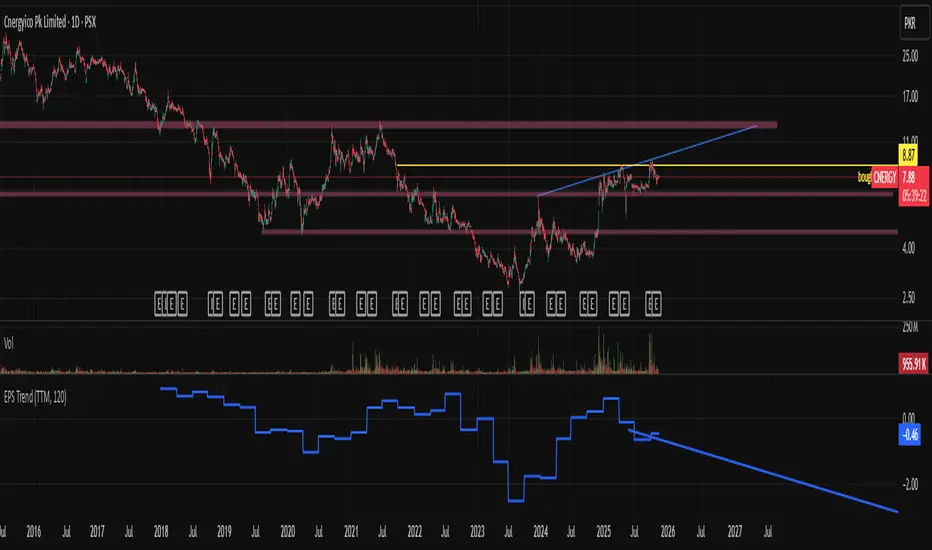
EPS Trendline (Fundamentals Insight by Mazhar Karimi)Overview
This indicator visualizes a company’s Earnings Per Share (EPS) data directly on the chart—pulled from TradingView’s fundamental database—and applies a dynamic linear regression trendline to highlight the long-term direction of earnings growth or decline.
It’s designed to help investors and quantitative traders quickly see how the company’s profitability (EPS) has evolved over time and whether it’s trending upward (growth), flat (stagnant), or downward (decline).
How it Works
Uses request.financial() to fetch EPS data (Diluted or Basic).
You can select whether to use TTM (Trailing Twelve Months), FQ (Fiscal Quarter), or FY (Fiscal Year) data.
The script fits a regression line (using ta.linreg) over a configurable window to visualize the underlying EPS trend.
Updates automatically when new financial data is released.
Inputs
EPS Period: Choose between FQ / FY / TTM
Use Diluted EPS: Toggle to compare Diluted vs. Basic EPS
Regression Window: Adjust how many bars are used to fit the trendline
Interpretation Tips
A rising trendline indicates earnings momentum and potential investor confidence.
A flat or declining trendline may warn of profitability slowdowns.
Combine with price action or valuation ratios (like P/E) for deeper analysis.
Works best on stocks or ETFs with fundamental data (not available for crypto or FX).
Suggestions / Use Cases
Pair with Price/Earnings ratio indicators to evaluate valuation vs. fundamentals.
Use in conjunction with earnings release events for context.
Ideal for long-term investors, swing traders, or fundamental quants tracking financial health trends.
Future Enhancements (Planned Ideas)
🔹 Option to display multiple regression lines (short-term and long-term)
🔹 Support for comparing multiple tickers’ EPS in the same pane
🔹 Integration with Net Income, Revenue, or Free Cash Flow trends
🔹 Add a “Rate of Change” signal for momentum-based EPS analysis
NY ORB - Full Dynamic SystemNY ORB - Full Dynamic Strategy Summary
1. Opening Range and Session Timing
Opening Range (ORB) Calculation: The strategy identifies the ORB High and ORB Low by tracking the highest high and lowest low during the specified New York pre-market window, which is set by default from 8:30 to 8:45 (New York time).
Entry Window: Trading activity is restricted to a specific entry period, typically starting shortly after the ORB is established (default: 8:50 to 12:00).
Hard Exit Time: Any remaining open positions are automatically closed at a fixed exit time (default: 13:25).
2. Trade Entry Logic and Filters
An entry (Long or Short) is generated when the price breaks out of the established ORB, provided it passes a series of optional filters:
Direction Control: The user can restrict the strategy to trade Long Only, Short Only, or Both.
Second Breakout Logic: An optional filter that requires the price to break out, reverse back into the range, and then break out again, confirming momentum after a consolidation.
Confirmation Candle Count: An optional filter that checks the close of a previous candle (e.g., 1 or 2 candles ago) to ensure the price was still inside the range, preventing premature entry.
Technical Filters (Optional): The entry is only executed if it aligns with selected indicators:
RSI: Filters for non-overbought (Long) or non-oversold (Short) conditions.
MACD: Requires the MACD line to be above/below the Signal line for alignment.
VWAP: Requires the price to be above/below the Volume-Weighted Average Price.
Trend Filter (SMMA): Requires the price to be above/below a 50-period Simple Moving Average.
3. Dynamic Risk and Exit Management
This strategy features highly configurable stop-loss and profit-taking mechanics:
Primary Stop Loss Methods: The Stop Loss distance can be dynamically chosen from four types:
Fixed: A fixed number of ticks.
ATR: Based on a multiple of the Average True Range (ATR).
Capped ATR: ATR-based, but with a hard maximum tick limit.
OR-Based: Based on a multiple of the actual ORB High-to-Low range.
Dynamic Profit Target: The Take Profit level is calculated dynamically based on a multiplier of either the ATR or the ORB Range.
Breakeven Stop:
If enabled, the Stop Loss automatically moves to the entry price (Breakeven) once the price moves a predetermined distance in the profitable direction.
An Adaptive Breakeven option allows the trigger distance to be calculated as a percentage of the overall ATR Profit Target.
Trailing Stop: The strategy uses a trailing stop, which can be custom-set (fixed ticks) or dynamically tied to the ATR. An optional feature Auto Tighten Trailing reduces the trailing multiplier once the breakeven level is hit.
MA Cross Exit: An alternative, counter-trend exit mechanism that closes the trade if the price crosses back over the chosen Moving Average (either SMMA or VWAP), overriding the pending profit target.
4. Daily Account Management
The strategy includes crucial daily risk controls to protect capital and lock in profits:
Daily Profit Limit: If the total daily PnL (realized and unrealized) hits a predefined maximum profit threshold (in ticks), all trades are closed, and new entries are blocked for the remainder of the trading day.
Daily Loss Limit: Conversely, if the total daily PnL hits a predefined maximum loss threshold, all trades are closed, and new entries are blocked for the remainder of the day.

saodisengxiaoyu-lianghua-2.1- This indicator is a modular, signal-building framework designed to generate long and short signals by combining a chosen leading indicator with selectable confirmation filters. It runs on Pine Script version 5, overlays directly on price, and is built to be highly configurable so traders can tailor the signal logic to their market, timeframe, and trading style. It includes a dashboard to visualize which conditions are active and whether they validate a signal, and it outputs clear buy/sell labels and alert conditions so you can automate or monitor trades with confidence.
Core Design
- Leading Indicator: You choose one primary signal generator from a broad list (for example, Range Filter, Supertrend, MACD, RSI, Ichimoku, and many others). This serves as the anchor of the system and determines when a preliminary long or short setup exists.
- Confirmation Filters: You can enable additional filters that validate the leading signal before it becomes actionable. Each “respect…” input toggles a filter on or off. These filters include popular tools like EMA, 2/3 EMA crosses, RQK (Nadaraya Watson), ADX/DMI, Bollinger-based oscillators, MACD variations, QQE, Hull, VWAP, Choppiness Index, Damiani Volatility, and more.
- Signal Expiry: To avoid waiting indefinitely for confirmations, the indicator counts how many consecutive bars the leading condition holds. If confirmations do not align within a defined number of bars, the setup expires. This controls latency and helps reduce late or stale entries.
- Alternating Signals: An optional mode enforces alternation (long must follow short and vice versa), helping avoid repeated entries in the same direction without a meaningful reset.
- Aggregation Logic: The final long/short conditions are formed by combining the leading condition with all selected confirmation filters through logical conjunction. Only if all enabled filters validate the signal (within expiry constraints) does the indicator consider it a confirmed long or short.
- Visualization and Alerts: The script plots buy/sell labels at signal points, provides alert conditions for automation, and displays a compact dashboard summarizing the leading indicator’s status and each confirmation’s pass/fail result using checkmarks.
Leading Indicator Options
- The indicator includes a very large menu of leading tools, each with its own logic to determine uptrend or downtrend impulses. Highlights include:
- Range Filter: Uses a dynamic centerline and bands computed via conditional EMA/SMA and range sizing to define directional movement. It can operate in a default mode or an alternative “DW” mode.
- Rational Quadratic Kernel (RQK): Applies a kernel smoothing model (Nadaraya Watson) to detect uptrends and downtrends with a focus on noise reduction.
- Supertrend, Half Trend, SSL Channel: Classic trend-following tools that derive direction from ATR-based bands or moving average channels.
- Ichimoku Cloud and SuperIchi: Multi-component systems validating trend via cloud position, conversion/base line relationships, projected cloud, and lagging span.
- TSI (True Strength Index), DPO (Detrended Price Oscillator), AO (Awesome Oscillator), MACD, STC (Schaff Trend Cycle), QQE Mod: Momentum and cycle tools that parse direction from crossovers, zero-line behavior, and momentum shifts.
- Donchian Trend Ribbon, Chandelier Exit: Trend and exit tools that can validate breakouts or sustained trend strength.
- ADX/DMI: Measures trend strength and directional movement via +DI/-DI relationships and minimum ADX thresholds.
- RSI and Stochastic: Use crossovers, level exits, or threshold filters to gate entries based on overbought/oversold dynamics or relative strength trends.
- Vortex, Chaikin Money Flow, VWAP, Bull Bear Power, ROC, Wolfpack Id, Hull Suite: A diverse set of directional, momentum, and volume-based indicators to suit different markets and styles.
- Trendline Breakout and Range Detector: Price-behavior filters that confirm signals during breakouts or within defined ranges.
Confirmation Filters
- Each filter is optional. When enabled, it must validate the leading condition for a signal to pass. Examples:
- EMA Filter: Requires price to be above a specified EMA for longs and below for shorts, filtering signals that contradict broader trend or baseline levels.
- 2 EMA Cross and 3 EMA Cross: Enforce moving average cross conditions (fast above slow for long, the reverse for short) or a three-line stacking logic for more stringent trend alignment.
- RQK, Supertrend, Half Trend, Donchian, QQE, Hull, MACD (crossover vs. zero-line), AO (zero line or AC momentum variants), SSL: Each adds its characteristic validation pattern.
- RSI family (MA cross, exits OB/OS zones, threshold levels) plus RSI MA direction and RSI/RSI MA limits: Multiple ways to constrain signals via relative strength behavior and trajectories.
- Choppiness Index and Damiani Volatility: Prevent entries during ranging conditions or insufficient volatility; choppiness thresholds and volatility states gate the trade.
- VWAP, Volume modes (above MA, simple up/down, delta), Chaikin Money Flow: Volume and flow conditions that ensure signals happen in supportive liquidity or accumulation/distribution contexts.
- ADX/DMI thresholds: Demand a minimum trend strength and directional DI alignment to reduce whipsaw trades.
- Trendline Breakout and Range Detector: Confirm that the price is breaking structure or remains within active range consistent with the leading setup.
- By combining several filters you can create strict, conservative entries or looser setups depending on your goals.
Range Filter Engine
- A core building block, the Range Filter uses conditional EMA and SMA functions to compute adaptive bands around a dynamic centerline. It supports two types:
- Type 1: The centerline updates when price exceeds the band thresholds; bands define acceptable drift ranges.
- Type 2: Uses quantized steps (via floor operations) relative to the previous centerline to handle larger moves in discrete increments.
- The engine offers smoothing for range values using a secondary EMA and can switch between raw and averaged outputs. Its hi/lo bands and centerline compose a corridor that defines directional movement and potential breakout confirmation.
Signal Construction
- The script computes:
- leadinglongcond and leadingshortcond : The primary directional signals from the chosen leading indicator.
- longCond and shortCond : Final signals formed by combining the leading conditions with all enabled confirmations. Each confirmation contributes a boolean gate. If a filter is disabled, it contributes a neutral pass-through, keeping the logic intact without enforcing that condition.
- Expiry Logic: The code counts consecutive bars where the leading condition remains true. If confirmations do not line up within the user-defined “Signal Expiry Candle Count,” the setup is abandoned and the signal does not trigger.
- Alternation: An optional state ensures that long and short signals alternate. This can reduce repeated entries in the same direction without a clear reset.
- Finally, longCondition and shortCondition represent the actionable signals after expiry and alternation logic. These drive the label plotting and alert conditions.
Visualization
- Buy and Sell Labels: When longCondition or shortCondition confirm, the script plots annotated labels directly on the chart, making entries easy to see at a glance. The labels use color coding and clear text tags (“long” vs. “short”).
- Dashboard: A table summarizes the status of the leading indicator and all confirmations. Each row shows the indicator label and whether it passed (✔️) or failed (❌) on the current bar. This intensely practical UI helps you diagnose why a signal did or did not trigger, empowering faster strategy iteration and parameter tuning.
- Failed Confirmation Markers: If a setup expires (count exceeds the limit) and confirmations failed to align, the script can mark the chart with a small label and provide a tooltip listing which confirmations did not pass. It’s a helpful audit trail to understand missed trades or prevent “chasing” invalid signals.
- Data Window Values: The script outputs signal states to the data window, which can be useful for debugging or building composite conditions in multi-indicator templates.
Inputs and Parameters
- You control the indicator from a comprehensive input panel:
- Setup: Signal expiry count, whether to enforce alternating signals, and whether to display labels and the dashboard (including position and size).
- Leading Indicator: Choose the primary signal generator from the large list.
- Per-Filter Toggles: For each confirmation, a respect... toggle enables or disables it. Many include sub-options (like MACD type, Stochastic mode, RSI mode, ADX variants, thresholds for choppiness/volatility, etc.) to fine-tune behavior.
- Range Filter Settings: Choose type and behavior; select default vs. DW mode and smoothing. The underlying functions adjust band sizes using ATR, average change, standard deviation, or user-defined scales.
- Because everything is customizable, you can adapt the indicator to different assets, volatility regimes, and timeframes.
Alerts and Automation
- The script defines alert conditions tied to longCondition and shortCondition . You can set these alerts in your chart to trigger notifications or webhook calls for automated execution in external bots. The alert text is simple, and you can configure your own message template when creating alerts in the chart, including JSON payloads for algorithmic integration.
Typical Workflow
- Select a Leading Indicator aligned with your style. For trend following, Supertrend or SSL may be appropriate; for momentum, MACD or TSI; for range/trend-change detection, Range Filter, RQK, or Donchian.
- Add a few key Confirmation Filters that complement the leading signal. For example:
- Pair Supertrend with EMA Filter and RSI MA Direction to ensure trend alignment and positive momentum.
- Combine MACD Crossover with ADX/DMI and Volume Above MA to avoid signals in low-trend or low-liquidity conditions.
- Use RQK with Choppiness Index and Damiani Volatility to only act when the market is trending and volatile enough.
- Set a sensible Signal Expiry Candle Count. Shorter expiry keeps entries timely and reduces lag; longer expiry captures setups that mature slowly.
- Observe the Dashboard during live markets to see which filters pass or fail, then iterate. Tighten or loosen thresholds and filter combinations as needed.
- For automation, turn on alerts for the final conditions and use webhook payloads to notify your trading robot.
Strengths and Practical Notes
- Flexibility: The indicator is a toolkit rather than a single rigid model. It lets you test different combinations rapidly and visualize outcomes immediately.
- Clarity: Labels, dashboard, and failed-confirmation markers make it easy to audit behavior and refine settings without digging into code.
- Robustness: The expiry and alternation options add discipline, avoiding the temptation to enter late or repeatedly in one direction without a reset.
- Modular Design: The logical gates (“respect…”) make the behavior transparent: if a filter is on, it must pass; if it’s off, the signal ignores it. This keeps reasoning clean.
- Avoiding Overfitting: Because you can stack many filters, it’s tempting to over-constrain signals. Start simple (one leading indicator and one or two confirmations). Add complexity only if it demonstrably improves your edge across varied market regimes.
Limitations and Recommendations
- No single configuration is universally optimal. Markets change; tune filters for the instrument and timeframe you trade and revisit settings periodically.
- Trend filters can underperform in choppy markets; likewise, momentum filters can false-trigger in quiet periods. Consider using Choppiness Index or Damiani to gate signals by regime.
- Use expiry wisely. Too short may miss good setups that need a few bars to confirm; too long may cause late entries. Balance responsiveness and accuracy.
- Always consider risk management externally (position sizing, stops, profit targets). The indicator focuses on signal quality; combining it with robust trade management methods will improve results.
Example Configurations
- Trend-Following Setup:
- Leading: Supertrend uptrend for longs and downtrend for shorts.
- Confirmations: EMA Filter (price above 200 EMA for long, below for short), ADX/DMI (trend strength above threshold with +DI/-DI alignment), Volume Above MA.
- Expiry: 3–4 bars to keep entries timely.
- Result: Strong bias toward sustained moves while avoiding weak trends and thin liquidity.
- Mean-Reversion to Momentum Crossover:
- Leading: RSI exits from OB/OS zones (e.g., RSI leaves oversold for long and leaves overbought for short).
- Confirmations: 2 EMA Cross (fast crossing slow in the same direction), MACD zero-line behavior for added momentum validation.
- Expiry: 2–3 bars for responsive re-entry.
- Result: Captures momentum transitions after short-term extremes, with extra confirmation to reduce head-fakes.
- Range Breakout Focus:
- Leading: Range Filter Type 2 or Donchian Trend Ribbon to detect breakouts.
- Confirmations: Damiani Volatility (avoid low-volatility false breaks), Choppiness Index (prefer trend-ready states), ROC positive/negative threshold.
- Expiry: 1–3 bars to act on breakout windows.
- Result: Better alignment to breakout dynamics, gating trades by volatility and regime.
Conclusion
- This indicator is a comprehensive, configurable framework that merges a chosen leading signal with an array of corroborating filters, disciplined expiry handling, and intuitive visualization. It’s designed to help you build high-quality entry signals tailored to your approach, whether that’s trend-following, breakout trading, momentum capturing, or a hybrid. By surfacing pass/fail states in a dashboard and allowing alert-based automation, it bridges the gap between discretionary analysis and systematic execution. With sensible parameter tuning and thoughtful filter selection, it can serve as a robust backbone for signal generation across diverse instruments and timeframes.

4-Hour Range Scalping [v6.3]User Guide: 4-Hour Range Scalping Strategy
Hello! Here is the guide for the Pine Script strategy. Please read it carefully to get the best results.
📈 This script automates the "4-Hour Range Scalping Strategy" from the video.
The main idea is that the first four hours of a major trading day (like New York) set up a "trap zone." The strategy waits for the price to break out of this zone and then fail, giving us a signal that the breakout was false and the price is likely to reverse.
Here’s the simple logic:
Define the Range: It precisely calculates the highest high and lowest low during the first four hours of the selected trading session (e.g., 00:00 to 04:00 New York Time).
Wait for a Breakout: It then monitors the 5-minute chart for a price breakout where a candle fully closes outside of this established range.
Identify the Reversal: The trade trigger occurs when the price fails to continue its breakout and a subsequent 5-minute candle closes back inside the range. This signals a potential reversal or "failed breakout."
Execute the Trade:
]A Short (Sell) trade is triggered after a failed breakout above the range high.
A Long (Buy) trade is triggered after a failed breakout below the range low.
Manage the Risk: The Stop Loss is automatically placed at the peak (for shorts) or trough (for longs) of the breakout move, and the Take Profit is set to a default 2:1 Risk/Reward Ratio.
How to Use the Script (Step-by-Step) ⚙️
Follow these instructions to get it running perfectly.
1. Set Your Chart Timeframe This is the most important step. The strategy is designed to run on a 5-minute (5m) chart. Open your TradingView chart and make sure the timeframe is set to "5m".
2. Add the Script to Your Chart Open the Pine Editor tab at the bottom of TradingView, paste the entire script, and click the "Add to chart" button.
3. Configure the Settings On your chart, find the strategy's name (e.g., "4-Hour Range Scalping ") and click the gear icon ⚙️ to open its settings.
Trading Session: Choose the session for the range. New York is the default and the one from the video.
Risk/Reward Ratio: The default is 2.0, meaning your potential profit is twice your potential loss. You can adjust this to test other targets.
Backtesting Period: To see how the strategy performed on all historical data, go to the "Strategy Tester" panel, click its own gear icon ⚙️, and uncheck the boxes for "Start Date" and "End Date."
4. Understand the Visuals on Your Chart
Blue Background Area: This is the 4-hour calculation window. The script is identifying the day's high and low during this time. No trades will ever happen here.
Red Line (Range High): The highest price of the 4-hour window. This is the upper boundary of the "trap zone."
Green Line (Range Low): The lowest price of the 4-hour window. This is the lower boundary.
Green Triangle (▲): Shows where a Long (Buy) trade was entered.
Red Triangle (▼): Shows where a Short (Sell) trade was entered.
A Very Important Note on Timezones 🕒
This is critical for you in the Philippines (PHT).
The script is based on the New York session, which is 12 hours behind you. Your TradingView chart will still show your local time, but the script works on NY time in the background.
The New York "day" begins at 12:00 PM (Noon) your time.
The script's blue calculation window will be from 12:00 PM to 4:00 PM your local time.
The red and green range lines will appear on your chart only after 4:00 PM your time.
So, if you look at your chart in the morning or early afternoon, you will not see today's range yet. This is normal! The script is just waiting for the New York session to start.
How to Set Up Trade Alerts 🔔
You can have TradingView send you a notification whenever the script enters a trade.
Click the "Alert" button (looks like a clock) in the right-hand toolbar of TradingView.
In the "Condition" dropdown, select the name of the script (e.g., "4-Hour Range Scalping...").
You will then see two options: "Long Signal" and "Short Signal".
Select one (e.g., "Long Signal") and configure how you want to be notified (e.g., "Notify on app").
Click "Create". Repeat the process to create an alert for the other signal.
⚠️ Important Disclosure
For Educational and Research Purposes Only.
This script and all accompanying information are provided for educational and research purposes only. The strategy demonstrated is a technical concept and should not be misconstrued as financial, investment, legal, or tax advice.
Trading financial markets involves substantial risk and is not suitable for every investor. There is a possibility that you could sustain a loss of some or all of your initial investment. Therefore, you should not invest money that you cannot afford to lose.
Past performance is not indicative of future results. The backtesting results shown by this script are historical and do not guarantee future performance. Market conditions are constantly changing.
By using this script, you acknowledge that you are solely responsible for any and all trading decisions you make. You should conduct your own thorough research and, if necessary, seek advice from an independent financial advisor before making any investment decisions. The creators of this script assume no liability for any of your trading results.

Multi Momentum 10/21/42/63 — Histogram + 2xSMAMY MM INDICATOR INDIRED BY KARADI
It averages four rate-of-change snapshots of price, all anchored at today’s close.
If “Show as %” is on, the value is multiplied by 100.
Each term is a simple momentum/ROC over a different lookback.
Combining 10, 21, 42, 63 bars blends short, medium, and intermediate horizons into one number.
Positive MM → average upward pressure across those horizons; negative MM → average downward pressure.
Why those lengths?
They roughly stack into ~2× progression (10→21≈2×10, 21→42=2×21, 63≈1.5×42). That creates a “multi-scale” momentum that’s less noisy than a single fast ROC but more responsive than a long ROC alone.
How to read the panel
Gray histogram = raw Multi-Momentum value each bar.
SMA Fast/Slow lines (defaults 12 & 26 over the MM values) = smoothing of the histogram to show the trend of momentum itself.
Typical signals
Zero-line context:
Above 0 → bullish momentum regime on average.
Below 0 → bearish regime.
Crosses of SMA Fast & Slow: momentum trend shifts (fast above slow = improving momentum; fast below slow = deteriorating).
Histogram vs SMA lines: widening distance suggests strengthening momentum; narrowing suggests momentum is fading.
Divergences: price makes a new high/low but MM doesn’t → potential exhaustion.
Compared to a classic ROC
A single ROC(20) is very sensitive to that one window.
MM averages several windows, smoothing idiosyncrasies (e.g., a one-off spike 21 bars ago) and reducing “lookback luck.”
Settings & customization
Lookbacks (10/21/42/63): you can tweak for your asset/timeframe; the idea is to mix short→medium horizons.
Percent vs raw ratio: percent is easier to compare across symbols.
SMA lengths: shorter = more reactive but choppier; longer = smoother but slower.
Practical tips
Use regime + signal: trade longs primarily when MM>0 and fast SMA>slow SMA; consider shorts when MM<0 and fast

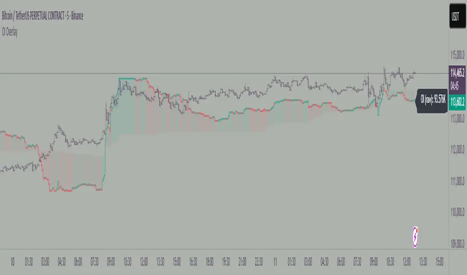
Open Interest OverlayOpen Interest Overlay
Overview
This indicator displays Open Interest (OI) data directly on your price chart as an overlay, eliminating the need for separate panes while preserving authentic OI movement patterns. Perfect for traders who want to analyze OI correlations without sacrificing chart real estate.
Key Features
📊 Smart Price Scaling
• Automatically maps Open Interest values to fit within your chart's price range
• Preserves all directional movements, timing, and relative magnitude relationships
• Uses official TradingView Open Interest feed for accuracy
🎨 Full Customization
• Custom Colors: Choose your own colors for rising/falling OI (defaults: teal/red)
• Line Style: Toggle between step-line (traditional) or smooth line display
• Optional Fill: Shade area between OI line and mid-price for better visual reference
• Smoothing Options: Apply moving average smoothing to reduce noise
⚙️ Intelligent Settings
• Normalization Window: 300-bar lookback (customizable) for scaling calculations
• Auto Timeframe: Uses daily data for intraday charts on traditional assets, chart timeframe for crypto
• Real Value Display: Shows actual (unscaled) OI value on the last bar
How It Works
The indicator performs proportional mapping of Open Interest data:
1. Calculates OI range (high/low) over the lookback period
2. Maps this range to your chart's price range during the same period
3. Displays OI movements that maintain authentic patterns and timing
Perfect For
✅ Correlation Analysis - See how OI moves with price in real-time
✅ Divergence Spotting - Identify when OI and price trends diverge
✅ Clean Charts - No need for separate panes or window splitting
✅ Pattern Recognition - Spot OI building/declining during key price levels
✅ Cross-Market Analysis - View any symbol's OI overlay on your current chart (e.g., Bitcoin OI while viewing Ethereum prices)
What You Get vs Traditional OI Indicators
Advantages:
• Authentic OI movement patterns preserved
• Direct visual correlation with price action
• No chart real estate sacrifice
• Immediate trend and divergence recognition
Trade-offs:
• Shows relative OI changes rather than absolute values
• Scaling is relative to the selected lookback period
Ideal For
• Day traders monitoring intraday OI flow
• Swing traders analyzing OI trends with price movements
• Futures traders tracking institutional interest
• Anyone wanting clean, correlation-focused OI analysis
Compatible With
• Futures contracts with Open Interest data
• Any timeframe (auto-adjusts for optimal data)
• All TradingView-supported OI symbols
AI-Weighted RSI (Zeiierman)█ Overview
AI-Weighted RSI (Zeiierman) is an adaptive oscillator that enhances classic RSI by applying a correlation-weighted prediction layer. Instead of looking only at RSI values directly, this indicator continuously evaluates how other price- and volume-based features (returns, volatility, volume shifts) correlate with RSI, and then weights them accordingly to project the next RSI state.
The result is a smoother, forward-looking RSI framework that adapts to market conditions in real time.
By leveraging feature correlation instead of static formulas, AI-Weighted RSI behaves like a lightweight learning model, adjusting its emphasis depending on which features are most aligned with RSI behavior during the current regime.
█ How It Works
⚪ Feature Extraction
Each bar, the script computes features: log returns, RSI itself, ATR% (volatility), volume, and volume log-change.
⚪ Correlation Screening
Over a rolling learning window, it measures the correlation of each feature against RSI. The strongest relationships are ranked and selected.
⚪ Adaptive Weighting
Features are standardized (z-scored), then combined using their signed correlations as weights, building a rolling, adaptive prediction of RSI.
⚪ Prediction to RSI Weight
The predicted RSI is mapped back into a “weight” scale (±2 by default). Above 0 = bullish bias, below 0 = bearish bias, with color-graded fills to visualize overbought/oversold pressure.
⚪ Signal Line
A smoothing option (signal length) overlays a moving average of the AI-Weighted RSI for clearer trend confirmation.
█ Why AI-Weighted RSI
⚪ Adaptive to Market Regime
Because the model re-evaluates correlations continuously, it naturally shifts which features dominate, sometimes volatility explains RSI best, sometimes volume, sometimes returns.
⚪ Forward-Looking Bias
Instead of simply reflecting RSI, the model provides a projection, helping anticipate shifts in momentum before RSI itself flips.
█ How to Use
⚪ Directional Bias
Read the RSI relative to 0. Above = bullish momentum bias, below = bearish.
⚪ Overbought / Oversold Zones
Shaded fills beyond +0.5 or -0.5 highlight extremes where RSI pressure often exhausts.
⚪ Divergences
When price makes new highs/lows but AI-Weighted RSI fails to confirm, it often signals weakening momentum.
█ Settings
RSI Length: Lookback for the core RSI calculation.
Signal Length: Smoothing applied to the AI-Weighted RSI output.
Learning Window: Bars used for correlation learning and z-scoring.
-----------------
Disclaimer
The content provided in my scripts, indicators, ideas, algorithms, and systems is for educational and informational purposes only. It does not constitute financial advice, investment recommendations, or a solicitation to buy or sell any financial instruments. I will not accept liability for any loss or damage, including without limitation any loss of profit, which may arise directly or indirectly from the use of or reliance on such information.
All investments involve risk, and the past performance of a security, industry, sector, market, financial product, trading strategy, backtest, or individual's trading does not guarantee future results or returns. Investors are fully responsible for any investment decisions they make. Such decisions should be based solely on an evaluation of their financial circumstances, investment objectives, risk tolerance, and liquidity needs.

Institutional Session VWAP Bands (Zeiierman)█ Overview
Institutional Session VWAP Bands (Zeiierman) plots a clean, session-aware VWAP that restarts at the “True Close” (end of the first trading hour) for each session you enable (Sydney, Tokyo, London, New York). From that anchor, the script computes a classic volume-weighted average price plus optional standard-deviation bands to frame session fair value and dispersion.
By aligning VWAP to when institutional flows settle (the first hour), you get a reference that matches real execution behavior, yielding more credible pullbacks, retests, and mean-reversion reads inside each session.
█ How It Works
⚪ Session Detection
You choose the sessions (on/off), their UTC-aligned time windows, and colors. The script detects when each session is active on your chart timeframe.
⚪ True-Close Anchoring
At session open the indicator waits. When the first hour completes, it flips the anchor on and starts a fresh VWAP for that session, mirroring how many desks treat the first hour as the real close for the prior day’s positioning.
⚪ VWAP Core
From the true-close anchor, VWAP is calculated in the standard way: cumulative (price × volume) / cumulative volume using your chosen price source (default hlc3).
⚪ VWAP Bands (σ)
Upper/Lower bands are built using a running standard deviation of the price source since the anchor. You control the σ multiplier and line width, and you can optionally fill between the bands.
█ Why Sessions + True-Close Anchoring
⚪ Institutional Timing Matters
A new anchor at the first-hour close reflects where real flows have settled, giving you a session fair-value line that aligns with how many funds evaluate prices intraday.
⚪ Cleaner Session Reads
Because VWAP and σ-bands restart each session, your retests, squeezes, and mean-reversion signals are based on today’s order-flow context, not yesterday’s inertia.
Result: a session-true fair-value with dispersion bands that stay close to the action, improving the quality of pullback entries and risk framing.
█ How to Use
⚪ Session Fair-Value Guide
Treat VWAP as the magnet for intraday value. Impulsive moves away from VWAP that fold back often present retest opportunities.
⚪ σ-Band Reversion & Breaks
Reversion: Tests beyond the upper/lower band that snap back inside can flag exhaustion.
Trend: Price riding the VWAP band in a strong trend
⚪ Session Handoffs
When one session hands to the next, watch how price behaves around the new session’s VWAP Bands after its anchor triggers. Continuation through the new VWAP vs. rejection often sets the tone.
█ Settings
UTC: Choose the timezone used to evaluate session windows (e.g., UTC+2).
Sessions (Sydney, Tokyo, London, New York): Toggle visibility and define each HHMM-HHMM window.
VWAP Price: Source for weighting.
Band Multiplier (σ): Standard deviation multiplier.
█ Related publications
True Close – Institutional Trading Sessions (Zeiierman)
-----------------
Disclaimer
The content provided in my scripts, indicators, ideas, algorithms, and systems is for educational and informational purposes only. It does not constitute financial advice, investment recommendations, or a solicitation to buy or sell any financial instruments. I will not accept liability for any loss or damage, including without limitation any loss of profit, which may arise directly or indirectly from the use of or reliance on such information.
All investments involve risk, and the past performance of a security, industry, sector, market, financial product, trading strategy, backtest, or individual's trading does not guarantee future results or returns. Investors are fully responsible for any investment decisions they make. Such decisions should be based solely on an evaluation of their financial circumstances, investment objectives, risk tolerance, and liquidity needs.

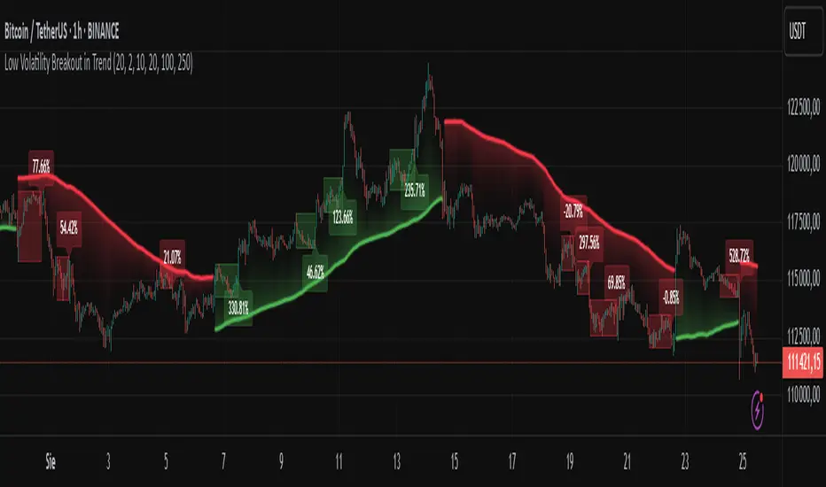
Low Volatility Breakout in Trend
█ OVERVIEW
"Low Volatility Breakout in Trend" is a technical analysis tool that identifies periods of low-volatility consolidation within an ongoing trend and signals potential breakouts aligned with the trend's direction. The indicator detects trends using a simple moving average (SMA) of price, identifies consolidation zones based on the size of candle bodies, and displays the percentage change in volume (volume delta) at the breakout moment.
█ CONCEPTS
The core idea of the indicator is to pinpoint moments where traders can join an ongoing trend by capitalizing on breakouts from consolidation zones, supported by additional information such as volume delta. It provides clear visualizations of trends, consolidation zones, and breakout signals to facilitate trading decisions.
Why Use It?
* Breakout Identification: The indicator locates low-volatility consolidation zones (measured by the size of individual candle bodies, not the price range of the consolidation) and signals breakouts, enabling traders to join the trend at key moments.
* Volume Analysis: Displays the percentage change in volume (delta) relative to its simple moving average, providing insight into market activity rather than acting as a signal filter.
* Visual Clarity: Colored trend lines, consolidation boxes (drawn only after the breakout candle closes, not on subsequent candles), and volume delta labels enable quick chart analysis.
* Flexibility: Adjustable parameters, such as the volatility window length or SMA period, allow customization for various trading strategies and markets.
How It Works
* Trend Detection: The indicator calculates a simple moving average (SMA) of price (default: based on the midpoint of high/low) and creates dynamic trend bands, offset by a percentage of the average candle height (band scaling). A price above the upper band signals an uptrend, while a price below the lower band indicates a downtrend. Trend changes occur not when the price crosses the SMA but when it crosses above the upper band or below the lower band (offset by the average candle height multiplied by the scaling factor).
* Consolidation Identification: Identifies low-volatility zones when the candle body size is smaller than the average body size over a specified period (default: 20 candles) multiplied by a volatility threshold — the maximum allowable body size as a percentage of the average body (e.g., 2 means the candle body must be less than twice the average body to be considered low-volatility).
* Breakout Signals: A breakout occurs when the candle body exceeds the volatility threshold, is larger than the maximum body in the consolidation, and aligns with the trend direction (bullish in an uptrend, bearish in a downtrend).
* Visualization: Draws a trend line with a gradient, consolidation boxes (appearing only after the breakout candle closes, marking the consolidation zone), and volume delta labels. Optionally displays breakout signal arrows.
* Signals and Alerts: The indicator generates signals for bullish and bearish breakouts, including the volume delta percentage. Alerts are an additional feature that can be enabled for notifications.
Settings and Customization
* Volatility Window: Length of the period for calculating the average candle body size (default: 20).
* Volatility Threshold: Maximum candle body size as a percentage of the average body (default: 2).
* Minimum Consolidation Bars: Number of candles required for a consolidation (default: 10).
* SMA Length for Trend: Period of the SMA for trend detection (default: 100).
* Band Scaling: Offset of trend bands as a percentage of the average candle height (default: 250%), determining the distance from the SMA.
* Visualization Options: Enable/disable consolidation boxes (Show Consolidation Boxes, drawn after the breakout candle closes), volume delta labels (Show Volume Delta Labels), and breakout signals (Show Breakout Signals, e.g., triangles).
* Colors: Customize colors for the trend line, consolidation boxes, and volume delta labels.
█ OTHER SECTIONS
Usage Examples
* Joining an Uptrend: When the price breaks out of a consolidation in an uptrend with a volume delta of +50%, open a long position; the signal is stronger if the breakout candle surpasses a local high.
* Avoiding False Breakouts: Ignore breakout signals with low volume delta (e.g., below 0%) and combine the indicator with other tools (e.g., support/resistance levels or oscillators) to confirm moves in low-activity zones.
Notes for Users
* On markets that do not provide volume data, the indicator will not display volume delta — disable volume labels and enable breakout signals (e.g., triangles) instead.
* Adjust parameters to suit the market's characteristics to minimize noise.
* Combine with other tools, such as Fibonacci levels or oscillators, for greater precision.
Indicador Millo SMA20-SMA200-AO-RSI M1This indicator is designed for scalping in 1-minute timeframes on crypto pairs, combining trend direction, momentum, and oscillator confirmation.
Logic:
Trend Filter:
Only BUY signals when price is above the SMA200.
Only SELL signals when price is below the SMA200.
Entry Trigger:
BUY: Price crosses above the SMA20.
SELL: Price crosses below the SMA20.
Confirmation Window:
After the price cross, the Awesome Oscillator (AO) must cross the zero line in the same direction within a maximum of N bars (configurable, default = 4).
RSI must be > 50 for BUY and < 50 for SELL at the moment AO confirms.
Cooldown:
A cooldown period (configurable, default = 10 bars) prevents multiple signals of the same type in a short time, reducing noise in sideways markets.
Features:
Works on any crypto pair and can be used in other markets.
Adjustable confirmation window, RSI threshold, and cooldown.
Alerts ready for BUY and SELL conditions.
Can be converted into a strategy for backtesting with TP/SL.
Suggested Use:
Pair: BTC/USDT M1 or similar high-liquidity asset.
Combine with manual support/resistance or higher timeframe trend analysis.
Recommended to confirm entries visually and with additional confluence before trading live.

Ichimoku Cloud Signals [sgbpulse] Ichimoku Cloud Signals – Your Advanced Trading Tool
Meet Ichimoku Cloud Signals, the enhanced and interactive version of the classic Ichimoku Cloud indicator, designed specifically for TradingView traders seeking precision and flexibility in their trading decisions. This indicator allows you to maximize the Ichimoku's potential by customizing trend criteria, receiving clear visual signals for entering and exiting positions, and getting alerts to keep you informed.
Introduction to the Ichimoku Cloud
The Ichimoku Cloud, also known as Ichimoku Kinko Hyo, is a comprehensive technical analysis tool developed in Japan. It provides a broad view of the market: trend direction, momentum, and support and resistance levels. "Ichimoku Cloud Signals" takes this power and amplifies it with advanced features.
Key Components of the Ichimoku Cloud
The indicator displays all five familiar Ichimoku lines, along with the "Cloud" (Kumo):
Tenkan-sen (Conversion Line): Calculated as the average of the highest high and lowest low over the past 9 periods. A fast, short-term indicator used as a measure of immediate momentum.
Kijun-sen (Base Line): Calculated as the average of the highest high and lowest low over the past 26 periods. A medium-term reference line serving as a significant support/resistance level.
Senkou Span A (Leading Span A): The average of the Tenkan-sen and Kijun-sen, shifted 26 periods forward into the future.
Senkou Span B (Leading Span B): The average of the highest high and lowest low over the past 52 periods, also shifted 26 periods forward into the future.
Kumo (Cloud): The area between Senkou Span A and Senkou Span B. Its color changes: green for an uptrend (when Senkou Span A is above Senkou Span B) and red for a downtrend (when Senkou Span B is above Senkou Span A). The Cloud serves as a dynamic area of support/resistance and a tool for forecasting future trends.
Chikou Span (Lagging Span): The current closing price, shifted 26 periods backward into the past. It serves as a powerful trend confirmation tool.
How the Ichimoku Cloud Works and How to Interpret It
Trend Identification :
- Uptrend (Bullish): The price is above the Cloud. The higher the price is above the Cloud, the stronger the trend.
- Downtrend (Bearish): The price is below the Cloud. The lower the price is below the Cloud, the stronger the trend.
- Range/Consolidation: The price is within the Cloud. This indicates a market without a clear direction or one that is consolidating.
Support and Resistance:
- The Cloud itself acts as a dynamic area of support and resistance. In an uptrend, the Cloud serves as support. In a downtrend, it serves as resistance.
- A thick Cloud indicates stronger support/resistance levels, while a thin Cloud indicates weaker levels.
The Cloud as a Predictive Indicator:
The uniqueness of the Kumo (Cloud) lies in its ability to be shifted 26 periods forward. This part of the Cloud provides forecasts for future support and resistance levels and even suggests expected trend changes (like a "Kumo Twist" – a change in Cloud color), giving you a planning advantage.
Unique Advantages of Ichimoku Cloud Signals:
Ichimoku Cloud Signals takes the classic Ichimoku principles and gives you unprecedented control:
Focused Trend Selection:
Choose whether you want to analyze a bullish (uptrend) or bearish (downtrend) trend. The indicator will focus on the relevant criteria for your selection.
Customizable Trend Confirmation Criteria (8 Criteria):
The indicator relies on 8 key criteria for clear trend confirmation. You can enable or disable each criterion individually based on your trading strategy and desired risk level. Each criterion plays a vital role in confirming the strength of the trend:
- Price position relative to the Cloud (Kumo) (Default: true): Determines the main trend direction and whether it's bullish or bearish.
- Price position relative to Kijun-sen (Base Line) (Default: true): Indicates the medium-term trend and acts as a critical equilibrium level.
- Price position relative to Tenkan-sen (Conversion Line) (Default: false): Provides quick confirmation of current momentum and short-term market changes.
- Tenkan-sen (Conversion Line) / Kijun-sen (Base Line) Crossover (Default: true): A classic signal for momentum change, crucial for identifying entry points.
- Current Cloud trend (Kumo) (Default: false): Cloud color confirms the main trend direction in real-time.
- Projected Future Cloud trend (Kumo) (Default: true): Indicates an expected future change in the Cloud's trend, providing strong visual insight.
- Chikou Span (Lagging Span) position relative to the Cloud (Kumo) (Default: true): Confirms the current trend strength by comparing the price to the Ichimoku 26 periods ago.
- Chikou Span (Lagging Span) position relative to the Price (Default: false): Additional confirmation of trend strength, indicating buyer/seller dominance.
Full Customization of Ichimoku Parameters:
You can change the period lengths for each Ichimoku component, depending on your strategy:
- Conversion Line Length (Default: 9)
- Base Line Length (Default: 26)
- Leading Span Length (Default: 52)
- Cloud Lagging Length (Default: 26)
- Lagging Span Length (Default: 26)
Visual Criteria Table on the Chart:
Get immediate and clear feedback! A visual table is placed on the chart, showing in real-time which of the 8 criteria you have defined are met for your chosen trend. Criteria you have enabled will be highlighted with a blue color and a "➤" symbol, while disabled criteria will appear in a subtle gray shade. For each criterion, the table shows its real-time status with a "✔" symbol if the condition is met and an "✘" symbol if it is not met. This powerful visual tool provides a quick assessment, helps with learning, and allows for strategy optimization at the click of a button.
Precise Criteria Details in the Data Window:
Beyond the visual table, the indicator provides an additional critical layer of detail: for any point on the chart, you can hover over a candle and see in TradingView's Data Window the precise status and values of all eight criteria. For each criterion, you'll see a clear numerical value (1 or 0) indicating whether it's fully met (1) or not met (0). Additionally, you can inspect the exact numerical values of the Ichimoku lines (Tenkan-sen, Kijun-sen, etc.) at that specific moment. This comprehensive data supports in-depth analysis, strategy debugging, and long-term optimization, providing complete transparency regarding every component of the signal.
Smart and Customizable Alerts:
Ichimoku Cloud Signals provides a powerful alert system to keep you informed of key market movements, so you never miss an opportunity. There are eight unique alerts you can enable in TradingView's alert panel:
Uptrend Entry Alert: Triggers when all of your selected criteria for an uptrend are met on a new candle.
Uptrend Exit Alert: Triggers when one of your selected uptrend criteria is no longer met, signaling a potential exit point.
Downtrend Entry Alert: Triggers when all of your selected criteria for a downtrend are met on a new candle.
Downtrend Exit Alert: Triggers when one of your selected downtrend criteria is no longer met, signaling a potential exit point.
Bullish Crossover Alert: Triggers when the Conversion Line (Tenkan-sen) crosses above the Base Line (Kijun-sen), a classic signal for an upward momentum shift.
Bearish Crossover Alert: Triggers when the Conversion Line (Tenkan-sen) crosses below the Base Line (Kijun-sen), signaling a potential shift to downward momentum.
Bullish Cloud Breakout Alert: Triggers when the price closes above the Ichimoku Cloud (Kumo), indicating a strong bullish trend.
Bearish Cloud Breakout Alert: Triggers when the price closes below the Ichimoku Cloud (Kumo), indicating a strong bearish trend.
Each alert can be independently configured in TradingView's alert panel, allowing you to tailor your notifications to fit your exact trading strategy and risk management preferences.
Summary:
Ichimoku Cloud Signals is an essential tool for TradingView traders seeking control, clarity, and precision. It combines the power of the classic Ichimoku Cloud indicator with advanced customization capabilities, a convenient visual table, and clear signals, empowering you to make informed trading decisions and stay focused on managing your positions.
Important Note: Trading Risk
This indicator is intended for educational and informational purposes only and does not constitute investment advice or a recommendation for trading in any form whatsoever.
Trading in financial markets involves significant risk of capital loss. It is important to remember that past performance is not indicative of future results. All trading decisions are your sole responsibility. Never trade with money you cannot afford to lose.

LANZ Strategy 5.0 [Backtest]🔷 LANZ Strategy 5.0 — Rule-Based BUY Logic with Time Filter, Session Limits and Auto SL/TP Execution
This is the backtest version of LANZ Strategy 5.0, built as a strategy script to evaluate real performance under fixed intraday conditions. It automatically places BUY and SELL trades based on structured candle confirmation, EMA trend alignment, and session-based filters. The system simulates real-time execution with precise Stop Loss and Take Profit levels.
📌 Built for traders seeking to simulate clean intraday logic with fully automated entries and performance metrics.
🧠 Core Logic & Strategy Conditions
✅ BUY Signal Conditions:
Price is above the EMA200
The last 3 candles are bullish (close > open)
The signal occurs within the defined session window (NY time)
Daily trade limit has not been exceeded
If all are true, a BUY order is executed at market, with SL and TP set immediately.
🔻 SELL Signal Conditions (Optional):
Exactly inverse to BUY (below EMA + 3 bearish candles). Disabled by default.
🕐 Operational Time Filter (New York Time)
You can fully customize your intraday window:
Start Time: e.g., 01:15 NY
End Time: e.g., 16:00 NY
The system evaluates signals only within this range, even across midnight if configured.
🔁 Trade Management System
One trade at a time per signal
Trades include a Stop Loss (SL) and Take Profit (TP) based on pip distance
Trade result is calculated automatically
Each signal is shown with a triangle marker (BUY only, by default)
🧪 Backtest Accuracy
This version uses:
strategy.order() for entries
strategy.exit() for SL and TP
strategy.close_all() at the configured manual closing time
This ensures realistic behavior in the TradingView strategy tester.
⚙️ Flow Summary (Step-by-Step)
On every bar, check:
Is the time within the operational session?
Is the price above the EMA?
Are the last 3 candles bullish?
If conditions met → A BUY trade is opened:
SL = entry – X pips
TP = entry + Y pips
Trade closes:
If SL or TP is hit
Or at the configured manual close time (e.g., 16:00 NY)
📊 Settings Overview
Timeframe: 1-hour (ideal)
SL/TP: Configurable in pips
Max trades/day: User-defined (default = 99 = unlimited)
Manual close: Adjustable by time
Entry type: Market (not limit)
Visuals: Plotshape triangle for BUY entry
👨💻 Credits:
💡 Developed by: LANZ
🧠 Strategy logic & execution: LANZ
✅ Designed for: Clean backtesting, clarity in execution, and intraday logic simulation

Price Statistical Strategy-Z Score V 1.01
Price Statistical Strategy – Z Score V 1.01
Overview
A technical breakdown of the logic and components of the “Price Statistical Strategy – Z Score V 1.01”.
This script implements a smoothed Z-Score crossover mechanism applied to the closing price to detect potential statistical deviations from local price mean. The strategy operates solely on price data (close) and includes signal spacing control and momentum-based candle filters. No volume-based or trend-detection components are included.
Core Methodology
The strategy is built on the statistical concept of Z-Score, which quantifies how far a value (closing price) is from its recent average, normalized by standard deviation. Two moving averages of the raw Z-Score are calculated: a short-term and a long-term smoothed version. The crossover between them generates long entries and exits.
Signal Conditions
Entry Condition:
A long position is opened when the short-term smoothed Z-Score crosses above the long-term smoothed Z-Score, and additional entry conditions are met.
Exit Condition:
The position is closed when the short-term Z-Score crosses below the long-term Z-Score, provided the exit conditions allow.
Signal Gapping:
A minimum number of bars (Bars gap between identical signals) must pass between repeated entry or exit signals to reduce noise.
Momentum Filter:
Entries are prevented during sequences of three or more consecutively bullish candles, and exits are prevented during three or more consecutively bearish candles.
Z-Score Function
The Z-Score is calculated as:
Z = (Close - SMA(Close, N)) / STDEV(Close, N)
Where N is the base period selected by the user.
Input Parameters
Enable Smoothed Z-Score Strategy
Enables or disables the Z-Score strategy logic. When disabled, no trades are executed.
Z-Score Base Period
Defines the number of bars used to calculate the simple moving average and standard deviation for the Z-Score. This value affects how responsive the raw Z-Score is to price changes.
Short-Term Smoothing
Sets the smoothing window for the short-term Z-Score. Higher values produce smoother short-term signals, reducing sensitivity to short-term volatility.
Long-Term Smoothing
Sets the smoothing window for the long-term Z-Score, which acts as the reference line in the crossover logic.
Bars gap between identical signals
Minimum number of bars that must pass before another signal of the same type (entry or exit) is allowed. This helps reduce redundant or overly frequent signals.
Trade Visualization Table
A table positioned at the bottom-right displays live PnL for open trades:
Entry Price
Unrealized PnL %
Text colors adapt based on whether unrealized profit is positive, negative, or neutral.
Technical Notes
This strategy uses only close prices — no trend indicators or volume components are applied.
All calculations are based on simple moving averages and standard deviation over user-defined windows.
Designed as a minimal, isolated Z-Score engine without confirmation filters or multi-factor triggers.
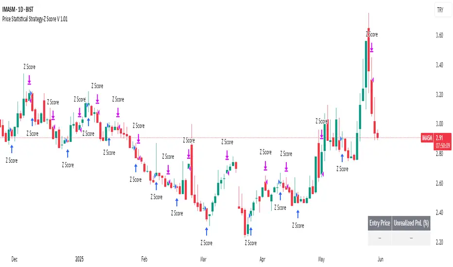
Tangent Extrapolation ForecastTangent Extrapolation Forecast
This indicator visually projects price direction by drawing a smoothed sequence of tangent lines based on recent price movements. For each bar in a user-defined lookback window, it calculates the slope over a smoothing period and extends the projected price forward. The resulting polyline forecast connect the endpoints of the extrapolations, and is color-coded to reflect directional changes: green for upward moves, red for downward, and gray for flat segments. This tool can assist traders in visualizing short-term momentum and potential trend continuity without introducing artificial future gaps.
Inputs:
Bars to Use: Number of historical bars used in the forecast.
Slope Smoothing Window: The number of bars used to calculate slope for projection.
Source: Price input for calculations (default is close).
This indicator does not generate buy/sell signals. It is intended as a visual aid to support discretionary analysis.

FibSync - DynamicFibSupportWhat is this indicator?
FibSync – DynamicFibSupport overlays your chart with both static and dynamic Fibonacci retracement levels, making it easy to spot potential areas of support and resistance.
Static Fibs: Calculated from the highest and lowest price over a user-defined lookback period.
Dynamic Fibs: Calculated from the most recent swing high and swing low, automatically adapting as new swings form.
How to use
Add the indicator to your chart.
Configure the settings:
Static Fib Period: Sets the lookback window for static fib levels.
Show Dynamic Fibonacci Levels: Toggle dynamic fibs on/off.
Dynamic Fib Swing Search Window: How far back to search for valid swing highs/lows.
Swing Strength (bars left/right): How many bars define a swing high/low (higher = stronger swing).
Interpret the levels:
Solid lines are static fibs.
Transparent lines are dynamic fibs (if enabled).
Colors match standard fib conventions (yellow = 0.236, red = 0.382, blue = 0.618, green = 0.786, gray = 0.5).
Tips
Static and dynamic fibs can overlap-this often highlights especially important support/resistance zones.
Adjust the swing strength for your trading style: lower values for short-term, higher for long-term swings.
Hide/show individual lines using the indicator’s style settings in TradingView.
Trading Ideas (for higher timeframes and static fibs)
Close above the blue line (0.618 static fib):
This can be interpreted as a potential long (buy) signal, suggesting the market is breaking above a key resistance level.
Close below the red line (0.382 static fib):
This can be interpreted as a potential short (sell) signal, indicating the market is breaking below a key support level.
Note: These signals are most meaningful on higher timeframes and when using the static fib lines. Always confirm with your own strategy and risk management.
