Bitcoin Power Law Bottom PriceThis is a super simplified version of Bitcoin Rainbow Wave script.
I removed everything except the power law bottom band.
Powerlaw

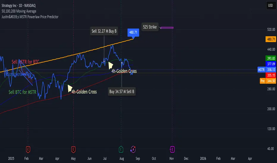
Justin's MSTR Powerlaw Price PredictorJustin's MSTR Powerlaw Price Predictor is a Pine Script v6 indicator for TradingView that adapts Giovanni Santostasi’s Bitcoin power law model to forecast MicroStrategy (MSTR) stock prices. The price prediction is based on the the formula published in this article:
www.ccn.com
BTC Power Law Valuation BandsBTC Power Law Rainbow
A long-term valuation framework for Bitcoin based on Power Law growth — designed to help identify macro accumulation and distribution zones, aligned with long-term investor behavior.
🔍 What Is a Power Law?
A Power Law is a mathematical relationship where one quantity varies as a power of another. In this model:
Price ≈ a × (Time)^b
It captures the non-linear, exponentially slowing growth of Bitcoin over time. Rather than using linear or cyclical models, this approach aligns with how complex systems, such as networks or monetary adoption curves, often grow — rapidly at first, and then more slowly, but persistently.
🧠 Why Power Law for BTC?
Bitcoin:
Has finite supply and increasing adoption.
Operates as a monetary network , where Metcalfe’s Law and power laws naturally emerge.
Exhibits exponential growth over logarithmic time when viewed on a log-log chart .
This makes it uniquely well-suited for power law modeling.
🌈 How to Use the Valuation Bands
The central white line represents the modeled fair value according to the power law.
Colored bands represent deviations from the model in logarithmic space, acting as macro zones:
🔵 Lower Bands: Deep value / Accumulation zones.
🟡 Mid Bands: Fair value.
🔴 Upper Bands: Euphoria / Risk of macro tops.
📐 Smart Money Concepts (SMC) Alignment
Accumulation: Occurs when price consolidates near lower bands — often aligning with institutional positioning.
Markup: As price re-enters or ascends the bands, we often see breakout behavior and trend expansion.
Distribution: When price extends above upper bands, potential for exit liquidity creation and distribution events.
Reversion: Historically, price mean-reverts toward the model — rarely staying outside the bands for long.
This makes the model useful for:
Cycle timing
Long-term DCA strategy zones
Identifying value dislocations
Filtering short-term noise
⚠️ Disclaimer
This tool is for educational and informational purposes only . It is not financial advice. The power law model is a non-predictive, mathematical framework and does not guarantee future price movements .
Always use additional tools, risk management, and your own judgment before making trading or investment decisions.

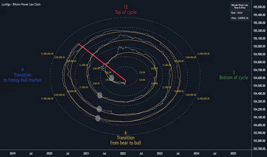
Bitcoin Power Law Clock [LuxAlgo]The Bitcoin Power Law Clock is a unique representation of Bitcoin prices proposed by famous Bitcoin analyst and modeler Giovanni Santostasi.
It displays a clock-like figure with the Bitcoin price and average lines as spirals, as well as the 12, 3, 6, and 9 hour marks as key points in the cycle.
🔶 USAGE
Giovanni Santostasi, Ph.D., is the creator and discoverer of the Bitcoin Power Law Theory. He is passionate about Bitcoin and has 12 years of experience analyzing it and creating price models.
As we can see in the above chart, the tool is super intuitive. It displays a clock-like figure with the current Bitcoin price at 10:20 on a 12-hour scale.
This tool only works on the 1D INDEX:BTCUSD chart. The ticker and timeframe must be exact to ensure proper functionality.
According to the Bitcoin Power Law Theory, the key cycle points are marked at the extremes of the clock: 12, 3, 6, and 9 hours. According to the theory, the current Bitcoin prices are in a frenzied bull market on their way to the top of the cycle.
🔹 Enable/Disable Elements
All of the elements on the clock can be disabled. If you disable them all, only an empty space will remain.
The different charts above show various combinations. Traders can customize the tool to their needs.
🔹 Auto scale
The clock has an auto-scale feature that is enabled by default. Traders can adjust the size of the clock by disabling this feature and setting the size in the settings panel.
The image above shows different configurations of this feature.
🔶 SETTINGS
🔹 Price
Price: Enable/disable price spiral, select color, and enable/disable curved mode
Average: Enable/disable average spiral, select color, and enable/disable curved mode
🔹 Style
Auto scale: Enable/disable automatic scaling or set manual fixed scaling for the spirals
Lines width: Width of each spiral line
Text Size: Select text size for date tags and price scales
Prices: Enable/disable price scales on the x-axis
Handle: Enable/disable clock handle
Halvings: Enable/disable Halvings
Hours: Enable/disable hours and key cycle points
🔹 Time & Price Dashboard
Show Time & Price: Enable/disable time & price dashboard
Location: Dashboard location
Size: Dashboard size
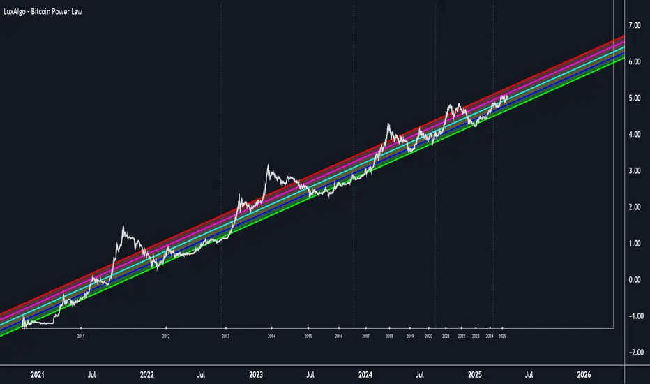
Bitcoin Power Law [LuxAlgo]The Bitcoin Power Law tool is a representation of Bitcoin prices first proposed by Giovanni Santostasi, Ph.D. It plots BTCUSD daily closes on a log10-log10 scale, and fits a linear regression channel to the data.
This channel helps traders visualise when the price is historically in a zone prone to tops or located within a discounted zone subject to future growth.
🔶 USAGE
Giovanni Santostasi, Ph.D. originated the Bitcoin Power-Law Theory; this implementation places it directly on a TradingView chart. The white line shows the daily closing price, while the cyan line is the best-fit regression.
A channel is constructed from the linear fit root mean squared error (RMSE), we can observe how price has repeatedly oscillated between each channel areas through every bull-bear cycle.
Excursions into the upper channel area can be followed by price surges and finishing on a top, whereas price touching the lower channel area coincides with a cycle low.
Users can change the channel areas multipliers, helping capture moves more precisely depending on the intended usage.
This tool only works on the daily BTCUSD chart. Ticker and timeframe must match exactly for the calculations to remain valid.
🔹 Linear Scale
Users can toggle on a linear scale for the time axis, in order to obtain a higher resolution of the price, (this will affect the linear regression channel fit, making it look poorer).
🔶 DETAILS
One of the advantages of the Power Law Theory proposed by Giovanni Santostasi is its ability to explain multiple behaviors of Bitcoin. We describe some key points below.
🔹 Power-Law Overview
A power law has the form y = A·xⁿ , and Bitcoin’s key variables follow this pattern across many orders of magnitude. Empirically, price rises roughly with t⁶, hash-rate with t¹² and the number of active addresses with t³.
When we plot these on log-log axes they appear as straight lines, revealing a scale-invariant system whose behaviour repeats proportionally as it grows.
🔹 Feedback-Loop Dynamics
Growth begins with new users, whose presence pushes the price higher via a Metcalfe-style square-law. A richer price pool funds more mining hardware; the Difficulty Adjustment immediately raises the hash-rate requirement, keeping profit margins razor-thin.
A higher hash rate secures the network, which in turn attracts the next wave of users. Because risk and Difficulty act as braking forces, user adoption advances as a power of three in time rather than an unchecked S-curve. This circular causality repeats without end, producing the familiar boom-and-bust cadence around the long-term power-law channel.
🔹 Scale Invariance & Predictions
Scale invariance means that enlarging the timeline in log-log space leaves the trajectory unchanged.
The same geometric proportions that described the first dollar of value can therefore extend to a projected million-dollar bitcoin, provided no catastrophic break occurs. Institutional ETF inflows supply fresh capital but do not bend the underlying slope; only a persistent deviation from the line would falsify the current model.
🔹 Implications
The theory assigns scarcity no direct role; iterative feedback and the Difficulty Adjustment are sufficient to govern Bitcoin’s expansion. Long-term valuation should focus on position within the power-law channel, while bubbles—sharp departures above trend that later revert—are expected punctuations of an otherwise steady climb.
Beyond about 2040, disruptive technological shifts could alter the parameters, but for the next order of magnitude the present slope remains the simplest, most robust guide.
Bitcoin behaves less like a traditional asset and more like a self-organising digital organism whose value, security, and adoption co-evolve according to immutable power-law rules.
🔶 SETTINGS
🔹 General
Start Calculation: Determine the start date used by the calculation, with any prior prices being ignored. (default - 15 Jul 2010)
Use Linear Scale for X-Axis: Convert the horizontal axis from log(time) to linear calendar time
🔹 Linear Regression
Show Regression Line: Enable/disable the central power-law trend line
Regression Line Color: Choose the colour of the regression line
Mult 1: Toggle line & fill, set multiplier (default +1), pick line colour and area fill colour
Mult 2: Toggle line & fill, set multiplier (default +0.5), pick line colour and area fill colour
Mult 3: Toggle line & fill, set multiplier (default -0.5), pick line colour and area fill colour
Mult 4: Toggle line & fill, set multiplier (default -1), pick line colour and area fill colour
🔹 Style
Price Line Color: Select the colour of the BTC price plot
Auto Color: Automatically choose the best contrast colour for the price line
Price Line Width: Set the thickness of the price line (1 – 5 px)
Show Halvings: Enable/disable dotted vertical lines at each Bitcoin halving
Halvings Color: Choose the colour of the halving lines
PLR-Z For Loop🧠 Overview
PLR-Z For Loop is a trend-following indicator built on the Power Law Residual Z-score model of Bitcoin price behavior. By measuring how far price deviates from a long-term power law regression and applying a custom scoring loop, this tool identifies consistent directional pressure in market structure. Designed for BTC, this indicator helps traders align with macro trends.
🧩 Key Features
Power Law Residual Model: Tracks deviations of BTC price from its long-term logarithmic growth curve.
Z-Score Normalization: Applies long-horizon statistical normalization (400/1460 bars) to smooth residual deviations into a usable trend signal.
Loop-Based Trend Filter: Iteratively scores how often the current Z-score exceeds prior values, emphasizing trend persistence over volatility.
Optional Smoothing: Toggleable exponential smoothing helps filter noise in choppier market conditions.
Directional Regime Coloring: Aqua (bullish) and Red (bearish) visuals reinforce trend alignment across plots and candles.
🔍 How It Works
Power Law Curve: Price is compared against a logarithmic regression model fitted to historical BTC price evolution (starting July 2010), defining structural support, resistance, and centerline levels.
Residual Z-Score: The residual is calculated as the log-difference between price and the power law center.
This residual is then normalized using a rolling mean (400 days) and standard deviation (1460 days) to create a long-term Z-score.
Loop Scoring Logic:
A loop compares the current Z-score to a configurable number of past bars.
Each higher comparison adds +1, and each lower one subtracts -1.
The result is a trend persistence score (z_loop) that grows with consistent directional momentum.
Smoothing Option: A user-defined EMA smooths the score, if enabled, to reduce short-term signal noise.
Signal Logic:
Long signal when trend score exceeds long_threshold.
Short signal when score drops below short_threshold.
Directional State (CD): Internally manages the current market regime (1 = long, -1 = short), controlling all visual output.
🔁 Use Cases & Applications
Macro Trend Alignment: Ideal for traders and analysts tracking Bitcoin’s structural momentum over long timeframes.
Trend Persistence Filter: Helps confirm whether the current move is part of a sustained trend or short-lived volatility.
Best Suited for BTC: Built specifically on the BNC BLX price history and Bitcoin’s power law behavior. Not designed for use with other assets.
✅ Conclusion
PLR-Z For Loop reframes Bitcoin’s long-term power law model into a trend-following tool by scoring the persistence of deviations above or below fair value. It shifts the focus from valuation-based mean reversion to directional momentum, making it a valuable signal for traders seeking high-conviction participation in BTC’s broader market cycles.
⚠️ Disclaimer
The content provided by this indicator is for educational and informational purposes only. Nothing herein constitutes financial or investment advice. Trading and investing involve risk, including the potential loss of capital. Always backtest and apply risk management suited to your strategy.

IlluminateThe Illuminate script predicts the potential range of Bitcoin's top and bottom prices based on a logarithmic regression model, referencing Bitcoin's historical price trends and halvings. This script is designed to provide valuable insights into Bitcoin's price dynamics and long-term trends using principles derived from the "Bitcoin Law."
Key Features
Power Law Trend Lines
Primary Trend:
Projects the general growth trajectory of Bitcoin prices over time based on a logarithmic power law.
Resistance Line:
Identifies a potential upper limit of Bitcoin prices during market peaks.
Includes an offset trendline for an additional buffer zone.
Support Line:
Represents a possible bottom for Bitcoin prices during market downturns.
Offset trendlines highlight potential zones of price fluctuation near the support line.
Fill Zones:
Between resistance and offset: Semi-transparent Red.
Between support and offset: Semi-transparent Green/Blue.
Bitcoin Halving Events
Automatically marks significant Bitcoin halving dates with yellow vertical lines and labeled annotations.
Current and future halvings (approximate) are included.
Trending Phase Indication
A dynamic visual color fill highlights different phases of Bitcoin's price evolution based on a 4-year cycle.
Colors: Red, Green, Blue, Orange (indicating each phase).
"Trending Phase" label provides insight into the current phase.
Interactive Inputs
Show/Hide Resistance: Toggle resistance trend lines.
Show/Hide Support: Toggle support trend lines.
Show/Hide Halving Dates: Toggle visibility of halving annotations.
Customizable Parameters
Fine-tune parameters (A and n) for the main trend line to match your analysis needs.
How to Use
Overlay Analysis:
Add this script to your TradingView chart for direct overlay on Bitcoin's price data.
Interpret the Zones:
Use the resistance and support lines as potential upper and lower bounds for price movements.
Analyze fill zones for areas of likely price oscillation.
Halving Significance:
Observe price behavior before and after halving dates, which historically influence market trends.
Long-Term Perspective:
The model is optimized for long-term projections, making it suitable for strategic, rather than short-term, trading decisions.
Disclaimer:
This indicator is for educational purposes only and should not be used as investment advice. Always do your own research and consult with a financial advisor before making trading decisions.

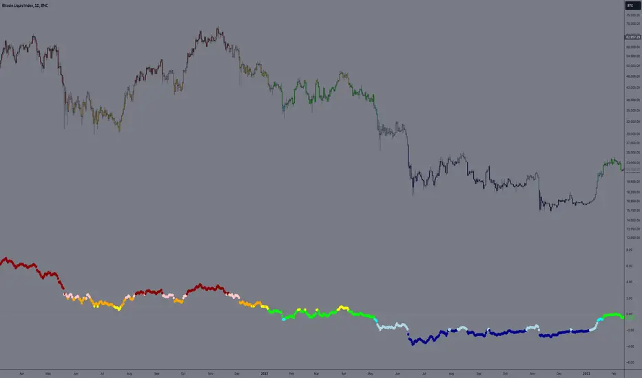
E9 PLRRThe E9 PLRR (Power Law Residual Ratio) is a custom-built indicator designed to evaluate the overvaluation or undervaluation of an asset, specifically by utilizing logarithmic price data and a power law-based model. It leverages a dynamic regression technique to assess the deviation of the current price from its expected value, giving insights into how much the price deviates from its long-term trend.
This indicator is primarily used to detect market extremes and cycles, often used in the analysis of long-term price movements in assets like Bitcoin, where cyclical behavior and significant price deviations are common.
This chart is back from 2019 and shows (From left to right) 2018 Bear market bottom at $3.5k (Dark Blue) , following a peak at 12k (dark red) before the Covid crash back down to EUROTLX:4K (Dark blue)
Key Components
Logarithmic Price Data:
The indicator works with logarithmic price data (ohlc4), which represents the average of open, high, low, and close prices. The logarithmic transformation is crucial in financial modeling, especially when analyzing long-term price data, as it normalizes exponential price growth patterns.
Dynamic Exponent 𝑘:
The model calculates a dynamic exponent k using regression, which defines the power law relationship between time and price. This exponent is essential in determining the expected power law price return and how far the current price deviates from that expected trend.
Power Law Price Return:
The power law price return is computed using the dynamic exponent
k over a defined period, such as 365 days (1 year). It represents the theoretical price return based on a power law relationship, which is used to compare against the actual logarithmic price data.
Risk-Free Rate:
The indicator incorporates an adjustable risk-free rate, allowing users to model the opportunity cost of holding an asset compared to risk-free alternatives. By default, the risk-free rate is set to 0%, but this can be modified depending on the user's requirements.
Volatility Adjustment:
A key feature of the PLRR is its ability to adjust for price volatility. The indicator smooths out short-term price fluctuations using a moving average, helping to detect longer-term cycles and trends.
PLRR Calculation:
The core of the indicator is the calculation of the Power Law Residual Ratio (PLRR). This is derived by subtracting the expected power law price return and risk-free rate from the logarithmic price return, then multiplying the result by a user-defined multiplier.
Color Gradient:
The PLRR values are represented visually using a color gradient. This gradient helps the user quickly identify whether the asset is in an undervalued, fair value, or overvalued state:
Dark Blue to Light Blue: Indicates undervaluation, with increasing blue tones representing a higher degree of undervaluation.
Green to Yellow: Represents fair value, where the price is aligned with the expected power law return.
Orange to Dark Red: Indicates overvaluation, with increasing red tones representing a higher degree of overvaluation.
Zero Line:
A zero line is plotted on the indicator chart, serving as a reference point. Values above the zero line suggest potential overvaluation, while values below indicate potential undervaluation.
Dots Visualization:
The PLRR is plotted using dots, with each dot color-coded based on the PLRR value. This dot-based visualization makes it easier to spot significant changes or reversals in market sentiment without overwhelming the user with continuous lines.
Bar Coloring:
The chart’s bars are colored in accordance with the PLRR value at each point in time, making it visually clear when an asset is potentially overvalued or undervalued.
Indicator Functionality
Cycle Identification : The E9 PLRR is especially useful for identifying cyclical market behavior. In assets like Bitcoin, which are known for their boom-bust cycles, the PLRR can help pinpoint when the market is likely entering a peak (overvaluation) or a trough (undervaluation).
Overvaluation and Undervaluation Detection: By comparing the current price to its expected power law return, the PLRR helps traders assess whether an asset is trading above or below its fair value. This is critical for long-term investors seeking to enter the market at undervalued levels and exit during periods of overvaluation.
Trend Following: The indicator helps users identify the broader trend by smoothing out short-term volatility. This makes it useful for both momentum traders looking to ride trends and contrarian traders seeking to capitalize on market extremes.
Customization
The E9 PLRR allows users to fine-tune several parameters based on their preferences or specific market conditions:
Lookback Period:
The user can adjust the lookback period (default: 100) to modify how the moving average and regression are calculated.
Risk-Free Rate:
Adjusting the risk-free rate allows for more realistic modeling of the opportunity cost of holding the asset.
Multiplier:
The multiplier (default: 5.688) amplifies the sensitivity of the PLRR, allowing users to adjust how aggressively the indicator responds to price movements.
This indicator was inspired by the works of Ashwin & PlanG and their work around powerLaw. Thank you. I hall be working on the calculation of this indicator moving forward to make improvements and optomisations.
BenfordsLawLibrary "BenfordsLaw"
Methods to deal with Benford's law which states that a distribution of first and higher order digits
of numerical strings has a characteristic pattern.
"Benford's law is an observation about the leading digits of the numbers found in real-world data sets.
Intuitively, one might expect that the leading digits of these numbers would be uniformly distributed so that
each of the digits from 1 to 9 is equally likely to appear. In fact, it is often the case that 1 occurs more
frequently than 2, 2 more frequently than 3, and so on. This observation is a simplified version of Benford's law.
More precisely, the law gives a prediction of the frequency of leading digits using base-10 logarithms that
predicts specific frequencies which decrease as the digits increase from 1 to 9." ~(2)
---
reference:
- 1: en.wikipedia.org
- 2: brilliant.org
- 4: github.com
cumsum_difference(a, b)
Calculate the cumulative sum difference of two arrays of same size.
Parameters:
a (float ) : `array` List of values.
b (float ) : `array` List of values.
Returns: List with CumSum Difference between arrays.
fractional_int(number)
Transform a floating number including its fractional part to integer form ex:. `1.2345 -> 12345`.
Parameters:
number (float) : `float` The number to transform.
Returns: Transformed number.
split_to_digits(number, reverse)
Transforms a integer number into a list of its digits.
Parameters:
number (int) : `int` Number to transform.
reverse (bool) : `bool` `default=true`, Reverse the order of the digits, if true, last will be first.
Returns: Transformed number digits list.
digit_in(number, digit)
Digit at index.
Parameters:
number (int) : `int` Number to parse.
digit (int) : `int` `default=0`, Index of digit.
Returns: Digit found at the index.
digits_from(data, dindex)
Process a list of `int` values and get the list of digits.
Parameters:
data (int ) : `array` List of numbers.
dindex (int) : `int` `default=0`, Index of digit.
Returns: List of digits at the index.
digit_counters(digits)
Score digits.
Parameters:
digits (int ) : `array` List of digits.
Returns: List of counters per digit (1-9).
digit_distribution(counters)
Calculates the frequency distribution based on counters provided.
Parameters:
counters (int ) : `array` List of counters, must have size(9).
Returns: Distribution of the frequency of the digits.
digit_p(digit)
Expected probability for digit according to Benford.
Parameters:
digit (int) : `int` Digit number reference in range `1 -> 9`.
Returns: Probability of digit according to Benford's law.
benfords_distribution()
Calculated Expected distribution per digit according to Benford's Law.
Returns: List with the expected distribution.
benfords_distribution_aprox()
Aproximate Expected distribution per digit according to Benford's Law.
Returns: List with the expected distribution.
test_benfords(digits, calculate_benfords)
Tests Benford's Law on provided list of digits.
Parameters:
digits (int ) : `array` List of digits.
calculate_benfords (bool)
Returns: Tuple with:
- Counters: Score of each digit.
- Sample distribution: Frequency for each digit.
- Expected distribution: Expected frequency according to Benford's.
- Cumulative Sum of difference:
to_table(digits, _text_color, _border_color, _frame_color)
Parameters:
digits (int )
_text_color (color)
_border_color (color)
_frame_color (color)

Bitcoin Power Law Bands (BTC Power Law) Indicator█ OVERVIEW
The 'Bitcoin Power Law Bands' indicator is a set of three US dollar price trendlines and two price bands for bitcoin , indicating overall long-term trend, support and resistance levels as well as oversold and overbought conditions. The magnitude and growth of the middle (Center) line is determined by double logarithmic (log-log) regression on the entire USD price history of bitcoin . The upper (Resistance) and lower (Support) lines follow the same trajectory but multiplied by respective (fixed) factors. These two lines indicate levels where the price of bitcoin is expected to meet strong long-term resistance or receive strong long-term support. The two bands between the three lines are price levels where bitcoin may be considered overbought or oversold.
All parameters and visuals may be customized by the user as needed.
█ CONCEPTS
Long-term models
Long-term price models have many challenges, the most significant of which is getting the growth curve right overall. No one can predict how a certain market, asset class, or financial instrument will unfold over several decades. In the case of bitcoin , price history is very limited and extremely volatile, and this further complicates the situation. Fortunately for us, a few smart people already had some bright ideas that seem to have stood the test of time.
Power law
The so-called power law is the only long-term bitcoin price model that has a chance of survival for the years ahead. The idea behind the power law is very simple: over time, the rapid (exponential) initial growth cannot possibly be sustained (see The seduction of the exponential curve for a fun take on this). Year-on-year returns, therefore, must decrease over time, which leads us to the concept of diminishing returns and the power law. In this context, the power law translates to linear growth on a chart with both its axes scaled logarithmically. This is called the log-log chart (as opposed to the semilog chart you see above, on which only one of the axes - price - is logarithmic).
Log-log regression
When both price and time are scaled logarithmically, the power law leads to a linear relationship between them. This in turn allows us to apply linear regression techniques, which will find the best-fitting straight line to the data points in question. The result of performing this log-log regression (i.e. linear regression on a log-log scaled dataset) is two parameters: slope (m) and intercept (b). These parameters fully describe the relationship between price and time as follows: log(P) = m * log(T) + b, where P is price and T is time. Price is measured in US dollars , and Time is counted as the number of days elapsed since bitcoin 's genesis block.
DPC model
The final piece of our puzzle is the Dynamic Power Cycle (DPC) price model of bitcoin . DPC is a long-term cyclic model that uses the power law as its foundation, to which a periodic component stemming from the block subsidy halving cycle is applied dynamically. The regression parameters of this model are re-calculated daily to ensure longevity. For the 'Bitcoin Power Law Bands' indicator, the slope and intercept parameters were calculated on publication date (March 6, 2022). The slope of the Resistance Line is the same as that of the Center Line; its intercept was determined by fitting the line onto the Nov 2021 cycle peak. The slope of the Support Line is the same as that of the Center Line; its intercept was determined by fitting the line onto the Dec 2018 trough of the previous cycle. Please see the Limitations section below on the implications of a static model.
█ FEATURES
Inputs
• Parameters
• Center Intercept (b) and Slope (m): These log-log regression parameters control the behavior of the grey line in the middle
• Resistance Intercept (b) and Slope (m): These log-log regression parameters control the behavior of the red line at the top
• Support Intercept (b) and Slope (m): These log-log regression parameters control the behavior of the green line at the bottom
• Controls
• Plot Line Fill: N/A
• Plot Opportunity Label: Controls the display of current price level relative to the Center, Resistance and Support Lines
Style
• Visuals
• Center: Control, color, opacity, thickness, price line control and line style of the Center Line
• Resistance: Control, color, opacity, thickness, price line control and line style of the Resistance Line
• Support: Control, color, opacity, thickness, price line control and line style of the Support Line
• Plots Background: Control, color and opacity of the Upper Band
• Plots Background: Control, color and opacity of the Lower Band
• Labels: N/A
• Output
• Labels on price scale: Controls the display of current Center, Resistance and Support Line values on the price scale
• Values in status line: Controls the display of current Center, Resistance and Support Line values in the indicator's status line
█ HOW TO USE
The indicator includes three price lines:
• The grey Center Line in the middle shows the overall long-term bitcoin USD price trend
• The red Resistance Line at the top is an indication of where the bitcoin USD price is expected to meet strong long-term resistance
• The green Support Line at the bottom is an indication of where the bitcoin USD price is expected to receive strong long-term support
These lines envelope two price bands:
• The red Upper Band between the Center and Resistance Lines is an area where bitcoin is considered overbought (i.e. too expensive)
• The green Lower Band between the Support and Center Lines is an area where bitcoin is considered oversold (i.e. too cheap)
The power law model assumes that the price of bitcoin will fluctuate around the Center Line, by meeting resistance at the Resistance Line and finding support at the Support Line. When the current price is well below the Center Line (i.e. well into the green Lower Band), bitcoin is considered too cheap (oversold). When the current price is well above the Center Line (i.e. well into the red Upper Band), bitcoin is considered too expensive (overbought). This idea alone is not sufficient for profitable trading, but, when combined with other factors, it could guide the user's decision-making process in the right direction.
█ LIMITATIONS
The indicator is based on a static model, and for this reason it will gradually lose its usefulness. The Center Line is the most durable of the three lines since the long-term growth trend of bitcoin seems to deviate little from the power law. However, how far price extends above and below this line will change with every halving cycle (as can be seen for past cycles). Periodic updates will be needed to keep the indicator relevant. The user is invited to adjust the slope and intercept parameters manually between two updates of the indicator.
█ RAMBLINGS
The 'Bitcoin Power Law Bands' indicator is a useful tool for users wishing to place bitcoin in a macro context. As described above, the price level relative to the three lines is a rough indication of whether bitcoin is over- or undervalued. Users wishing to gain more insight into bitcoin price trends may follow the author's periodic updates of the DPC model (contact information below).
█ NOTES
The author regularly posts on Twitter using the @DeFi_initiate handle.
█ THANKS
Many thanks to the following individuals, who - one way or another - made the 'Bitcoin Power Law Bands' indicator possible:
• TradingView user 'capriole_charles', whose open-source 'Bitcoin Power Law Corridor' script was the basis for this indicator
• Harold Christopher Burger, whose Bitcoin’s natural long-term power-law corridor of growth article (2019) was the basis for the 'Bitcoin Power Law Corridor' script
• Bitcoin Forum user "Trololo", who posted the original power law model at Logarithmic (non-linear) regression - Bitcoin estimated value (2014)

BTC Power Law HistogramBased on "Bitcoin’s natural long-term power-law corridor of growth" by Harold Christopher Burger

Bitcoin Power Law CorridorOpen-source live tracker of Harold Burger's Bitcoin "Power Law Corridor".
Added optional chart fill and labels to show the percentage delta to the regression center-line, support and resistance.

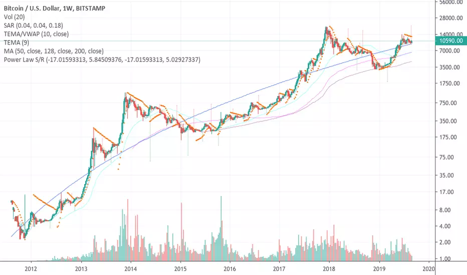
Power Law S/RBerger's article on the Power Law Model for Bitcoin is a compelling read and gives the best evidence so far of the diminishing case for retracing below $3000, of a slowing market on a log-log plot, and reducing but continued volatility.
After seeing it acts as support routinely in the last 10 years, I put together a quick little script that plots his midline curve for Bitcoin. You can change the intercept and slope but will need to do your own calculations for other curves.
I hope you all like it.
