Microstructure Participation & Acceptance Indicator📊 Microstructure Participation & Acceptance Indicator
An advanced participation-based filter combining VWAP distance analysis, volume delta detection, and real-time acceptance/rejection state identification—designed for smaller timeframe trading.
📊 FEATURES
VWAP Distance Normalization
Context-aware fair value measurement:
Automatically resets based on selected anchor (Session/Week/Month)
ATR-normalized distance calculation for universal application
Identifies when price is extended or compressed relative to equilibrium
Configurable extreme distance threshold (default: 1.5 ATR)
Adjustable source input (default: HLC3)
Volume Delta Proxy
Bull vs Bear participation tracking:
Calculates volume imbalance between bullish and bearish candles
EMA smoothing for cleaner signal generation (default: 9 periods)
Delta ratio measurement to identify dominant side
Expansion/compression detection to gauge momentum commitment
Configurable expansion threshold (default: 1.3x)
Acceptance/Rejection State Machine
Real-time market regime identification with six distinct states:
🟢 Accepted Long
Price moving away from VWAP with expanding bullish delta
Distance from VWAP increasing
Volume confirming the move
Indicates real buying pressure—trade WITH the move
🟢 Accepted Short
Price moving away from VWAP with expanding bearish delta
Distance from VWAP increasing
Volume confirming the move
Indicates real selling pressure—trade WITH the move
🟠 Fade Long
Price extended beyond threshold (>1.5 ATR above VWAP)
Delta not supporting the extension
Volume participation absent or diminishing
Potential mean-reversion short setup
🟠 Fade Short
Price extended beyond threshold (>1.5 ATR below VWAP)
Delta not supporting the extension
Volume participation absent or diminishing
Potential mean-reversion long setup
⚪ Chop
Price compressed near VWAP
Bollinger Bands tight (width compressed)
Delta neutral—no clear commitment
NO TRADE ZONE—wait for expansion
⚪ Neutral
Transitional state between regimes
Momentum shifting but not yet confirmed
Monitor for next acceptance signal
Bollinger Bands
Standard volatility measurement with TradingView default styling:
Adjustable period length (default: 20)
Configurable standard deviation multiplier (default: 2.0)
Visual fill between bands for volatility context
Used internally for chop/compression detection
Live Dashboard
Real-time metrics display (top-right corner):
Current market state with color coding
VWAP distance in ATR units
Delta ratio (bull/bear volume balance)
Delta state (Expanding/Compressing)
High-contrast design for instant readability
🎯 HOW TO USE
For Trend Trading:
Accepted Long/Short backgrounds indicate confirmed participation—stay with the trend
Strong moves typically travel 1-1.5 ATR from VWAP with delta support
Use VWAP as dynamic support/resistance
Combine with momentum indicators (MACD, RSI) for confluence
Price above VWAP + Accepted Long state = bullish bias
Price below VWAP + Accepted Short state = bearish bias
For Mean Reversion:
Fade Long/Short states signal overextension without participation
Price beyond 1.5 ATR from VWAP with weak delta = potential reversal
Look for price return to VWAP when extended
Bollinger Band extremes + Fade state = high-probability mean reversion setup
VWAP acts as mean reversion anchor during range-bound sessions
For Risk Management:
Chop state = avoid new entries
Bollinger Band compression + Chop = pre-expansion zone (wait for breakout)
Delta compression after strong move = early exhaustion warning
State transitions (Accepted → Neutral → Fade) = tighten stops
Signal Confirmation:
Strongest setups occur when multiple factors align:
BB breakout + Accepted state + price above/below VWAP
Price rejection at BB bands + Fade state
VWAP support/resistance hold + state transition
Delta expansion + distance increasing + trend direction
⚙️ SETTINGS
All components are fully customizable through organized input groups:
VWAP Distance Group:
VWAP source (default: HLC3)
Anchor period (Session/Week/Month)
ATR length for normalization (default: 14)
Extreme distance threshold in ATR multiples (default: 1.5)
Volume Delta Group:
Delta EMA length (default: 9)
Delta expansion threshold (default: 1.3)
Acceptance Logic Group:
Acceptance lookback period (default: 5)
Chop threshold in VWAP/ATR units (default: 0.3)
Bollinger Bands Group:
BB length (default: 20)
Standard deviation multiplier (default: 2.0)
Display Group:
Toggle state backgrounds
Toggle state change labels
Toggle VWAP line
Toggle Bollinger Bands
💡 EDUCATIONAL VALUE
This indicator teaches important concepts:
How institutional money identifies fair value (VWAP)
The difference between price movement and market acceptance
Why volume participation matters more than price action alone
How to distinguish between noise and committed directional moves
The relationship between volatility compression and expansion cycles
Why distance from equilibrium predicts mean reversion probability
⚠️ IMPORTANT NOTES
This indicator is for educational and informational purposes only
This is a filter, not a standalone trading system
No indicator is perfect—always use proper risk management
Past performance does not guarantee future results
Combine with your own analysis and risk tolerance
Test thoroughly on historical data before live trading
This is not financial advice—use at your own risk
🔧 TECHNICAL DETAILS
Pine Script Version 6
Overlay indicator (displays on price chart)
All calculations use standard, well-documented formulas
No repainting—all signals are confirmed on bar close
Compatible with all timeframes and instruments
Optimized for smaller timeframes (1-5 minute charts)
Minimal computational overhead
📝 CHANGELOG
Version 1.0
Initial release
VWAP distance normalization with ATR scaling
Volume delta proxy system (bull/bear EMA)
6-state acceptance/rejection state machine
Bollinger Bands integration
Real-time dashboard with live metrics
State change labels and background coloring
Full customization options
Developed for traders who need objective participation filters to distinguish high-probability setups from low-quality noise—without cluttering their charts with multiple indicator panels.
Meanreversion

Session ATR Progression Tracker📊 Session ATR Progression Tracker - SIYL Regression Trading Tool
Track how much of your instrument's 7-day Average True Range (ATR) has been covered during the current trading session. This indicator is specifically designed for regression traders who follow the "Stay In Your Lane" (SIYL) methodology, helping you identify when the probability of mean reversion significantly increases. If you are interested in more on that check out Rod Casselli and tradersdevgroup.com.
🎯 Key Features:
• Real-time ATR Coverage Percentage - See at a glance what percentage of the 7-day ATR has been covered in the current session
• SIYL-Optimized Thresholds - See at a glance when the instrument has achieved 80% and 100% ATR coverage, the proven thresholds where mean reversion probability increases (customizable)
• Flexible Session Modes:
- Daily: Resets at calendar day change
- Session: Uses exchange-defined trading sessions
- Custom Session: Set your exact session start/end times (perfect for futures traders and international markets)
• Visual Alerts - Color-coded display (gray → orange → red) and optional background highlighting
• Repositionable Display - Choose from 9 screen positions to avoid chart clutter
• Session Markers - Green triangles mark the start of each new session
• Detailed Stats - View current range, ATR value, session high/low, and session status
💡 Why Use This Indicator?
This tool is built around a proven concept: regression trading becomes significantly more effective once a session has achieved at least 80% of its 7-day ATR. At this threshold, the probability of price reverting to mean increases substantially, creating higher-probability trade setups for SIYL practitioners.
Benefits for regression traders:
- Identify optimal entry points when mean reversion probability is highest (≥80% ATR coverage)
- Avoid premature regression entries before adequate range has been established
- Recognize when daily moves have "earned their range" and are ripe for reversal
- Time fade-the-move and counter-trend strategies with statistical backing
- Improve win rates by trading only after proven probability thresholds are met
⚙️ Setup Instructions:
1. Add the indicator to your chart
2. Select your preferred "Reset Mode" (recommend "Custom Session" for futures/international markets)
3. If using Custom Session, enter your session times in 24-hour format (e.g., 0930-1600 for US stocks, 1700-1600 for CME futures)
4. Adjust alert thresholds if desired (default: 80% and 100% - proven SIYL thresholds)
5. Position the display where it's most visible on your chart
📈 Works Across All Markets:
Stocks • Futures • Forex • Indices • Crypto • Commodities
Perfect for regression traders, mean reversion specialists, and SIYL practitioners who want to trade with probability on their side by entering only after the session has "earned its range."
---
Tip: For futures contracts with overnight sessions that span calendar days (like MES, MNQ, MYM), use "Custom Session" mode with your exchange's official session times for accurate tracking.

Pulsar Heatmap CVD/OBV [by Oberlunar]Pulsar Heatmap CVD/OBV by Oberlunar is a non-repainting order-flow-like indicator designed to support fast, practical decisions—especially for day trading and scalping. It blends OBV and CVD into a structured heatmap with three lanes (OBV, CVD, and a blended COMBO) and splits each lane into two halves: flow pressure and price reaction (PriceΔ) . All values are normalised into the same range, so the intensity of each component is easy to compare at a glance.
In a simple sense, Pulsar Heatmap aims to provide a clean, integrated order-flow view: one framework that turns well-known volume concepts into a clearer read of market pressure and response. Personally, it feels like the kind of tool I would have always wanted on my chart, because it brings familiar information together into a more organic picture that is easier to use in real time.
Visually, the indicator is built around three main elements: the heatmap lanes , a pulsing triangle HUD , and a timed dashboard table . Under the hood, it follows a clear hierarchy: a Bias layer (directional context with a confidence percentage), a strict Signal layer (triggered only when full alignment occurs, with optional confirmation and stickiness), and optional timing logic based on ROC + Acceleration to validate impulses and highlight potential Exhaustion or Absorption regimes. With the option "Safe Mode" enabled, calculations update only on confirmed bars, so signals remain stable and do not repaint.
Optionally, the script can also print signal arrows/labels on the main chart only when a real Signal triggers (not when you only have Bias). To keep the chart clean, the same-direction label is not repeated unless the next signal appears at a more advantageous price than the previous one (for shorts: a higher price; for longs: a lower price). If the direction flips (SHORT → LONG or LONG → SHORT), label printing is re-enabled immediately.
What makes Pulsar Heatmap feel different is that it doesn’t leave you with two separate lines and a lot of guesswork. It organises the information into a readable decision map: pressure , response , agreement , disagreement , impulse , and timing . It was built with scalping in mind, but it’s not limited to scalping: the structure is useful whenever you want context first, and a strict trigger only when alignment is truly present.
Clean Trend Alignment (Ideal Continuation)
A “best case” scenario where flow and price response agree across lanes, so the system produces a high-confidence direction and a clean trigger. Show the heatmap with consistent colouring, the Bias band strong, and a confirmed signal/bias.
Setup 1 — Long Signal (Clean Alignment + Impulse)
In this example, Pulsar Heatmap transitions into a clear long setup when the system prints a LONG SIGNAL . The key idea is simple: the indicator does not enter on “bias” alone. It waits for full alignment across the internal lanes, optionally reinforced by the ROC/Acceleration impulse layer, and only then does it confirm a signal on a closed bar (Safe Mode).
What to highlight on the screenshot
The LONG SIGNAL label: this is the only moment the setup is considered “triggered”.
The LONG BIAS % label: this is context (direction + confidence), not the trigger.
The Triangle HUD : it visually summarises which component is driving the move (OBV/CVD/COMBO weight).
The Timed Table : show that Exhaustion is OFF while impulse metrics are supportive ( dynROC U and dynACC U positive).
If present, the Absorption state (e.g., ABS_LONG + “tight range”): it often appears during compression before expansion, and it adds context to why the breakout can accelerate.
How to read this long setup
Context : Bias is long (even if the % is not huge yet), and the system is not showing exhaustion.
Trigger : A LONG SIGNAL appears only after full alignment (with confirmation bars). If dynamic gating is enabled, the signal is valid only when the impulse agrees.
Quality checks : Positive dynROC and dynACC support the timing; absence of exhaustion reduces the risk of “late entry”. Absorption/tight range can indicate a “pressure build-up” phase.
Practical scalping execution (simple rule set)
Entry timing: consider the entry only on (or immediately after) the confirmed LONG SIGNAL candle.
Risk idea: invalidate the setup if the signal flips, or if price falls back into the compression/range that preceded the move (common absorption-breakout logic).
Exit clue: if Exhaustion turns ON or impulse weakens (acceleration flips), treat it as a warning to reduce exposure or take profit.
Setup 2 — Short Signal After Compression (Absorption → Release)
In this screenshot the short trade idea is not coming from “red candles” alone, but from a very specific sequence: the heatmap shows a shift into bearish alignment, the system prints a SHORT SIGNAL , and the timed module confirms that the market was in a tight range while sell pressure started to dominate.
What this image is really showing
You have a SHORT SIGNAL label on the chart: this is the trigger moment (not the bias).
The context reads SHORT BIAS 18% : it’s supportive, but the execution decision is driven by the signal.
The table shows Absorption = SHORT with a tight range (Range % is low): this often means price was compressed while one side kept applying pressure.
dyn metrics are negative ( dynROC U < 0 and dynACC U < 0): the impulse is coherent with the short direction, so the move is not just “random drift.”
How to read the heatmap here
Earlier, the lanes are mixed (more “two-sided”), then near the signal, the heatmap becomes decisively bearish. That change matters: it tells you the market stopped being balanced and started leaning in one direction with better internal coherence.
Why is this short “high quality” in scalping terms
Compression first : absorption/tight range means the market was storing energy.
Alignment next : the signal appears when the internal lanes agree.
Impulse last : negative ROC + negative acceleration support a real downside push, reducing the odds of a weak, slow fade.
Simple ensure-you-don’t-overtrade rule
Treat the SHORT SIGNAL as the only “go” moment. If you only see bias without signal, or the heatmap stays mixed/disagreeing, it’s usually a lower-quality scalp environment.
Disagreement Zone (Mixed Votes, Higher Risk) — A Practical Exit Area
In this screenshot, Pulsar Heatmap is clearly warning that the market is no longer “one-sided”. You can still see a directional context ( SHORT BIAS 11% ), but the key message is the DISAGREE tag: the reminder that the internal votes are split and the flow/price components are no longer moving in a clean, coherent way.
What this means in a trend continuation is very practical: a Disagreement Zone is often a good EXIT area . When you are already in a short trend, this is the moment where continuation becomes less reliable and where the market can start rotating, stalling, or snapping back.
Why it works as an exit trigger
In a healthy continuation, the lanes tend to stay aligned. Here they don’t: one or more halves contradict the dominant direction.
That loss of coherence typically shows up before the chart becomes obvious, so it can act as an early warning.
For scalping, this is where risk/reward often deteriorates: spreads, noise, and whipsaws increase exactly when the indicator starts disagreeing.
How to use it in a simple way
If you are already short , treat DISAGREE as a signal to take profit, tighten the stop, or scale out .
Avoid adding to the position inside disagreement: even if bias remains short, the internal structure is not “clean” enough to justify aggressive continuation entries.
If later the heatmap returns to full alignment and a new SHORT SIGNAL appears (ideally at a better price), then the continuation becomes actionable again.
“DISAGREE during a short continuation: coherence breaks down. In practice, this is often an exit/scale-out zone, not a fresh entry zone.”
Setup 3 — Neutral State (Stand-By Zone, No Trade Yet)
In the following screenshot, Pulsar Heatmap is doing something very important: it is clearly saying NEUTRAL 0% . Even if, visually, price could “look” like it might resume upward, the indicator is not providing a directional edge yet. This is a classic stand-by condition: the market is transitioning, and the internal components are not aligned enough to justify a directional scalp.
“Neutral 0%: mixed votes and no dominant driver. Even if the price looks promising, Pulsar stays in stand-by until bias rebuilds and a confirmed signal appears.”
What to highlight on the screenshot
The centre label NEUTRAL 0% : this is the key message—no bias strength worth following.
The heatmap is mixed/transitioning: lanes are not consistently one colour, meaning votes are not coherent.
The triangle HUD sits close to the centre: it visually reflects “no dominant driver” right now.
The table can still show background context (e.g., Absorption with a tight range), but that does not override neutrality: it’s information, not a trigger.
How to interpret “Neutral” in practice
When the indicator is neutral, it means the system sees a balance between pressure and reaction (or conflicting components), so direction is statistically less reliable. In scalping terms, this is usually where spreads and noise can eat you alive if you force entries.
Why this is still useful (even without a trade)
Neutral is not “nothing”—it is a filter. It prevents you from trading when the signal quality is low, and it forces the workflow to be clean: wait for Bias to build, then wait for a confirmed Signal , and only then treat it as a real setup.
What you wait for next
If the market turns bullish again, you want to see heatmap alignment returning and eventually a confirmed LONG SIGNAL —however, in the following examples, the heatmap does not follow the trade completely (unlike the previous generated long signal). Thus, a long entry is very risky.
If the market rolls over, you want the opposite: bearish alignment and a confirmed SHORT SIGNAL . Until one of these happens, Neutral = stand-by .
Setup 4 — Impulse + Exhaustion (Late-Stage Move, Don’t Chase)
In this screenshot, you’re basically seeing a “timing warning” configuration. Price prints a sharp bearish extension, but Pulsar Heatmap is not presenting it as a clean continuation setup: the center read is NEUTRAL 0% , while the timed engine shows both Absorption = SHORT and Exhaustion = SHORT . That combination often means: the downside pressure was real, but the move is already in a late/fragile phase (good for managing an existing short, not for opening a new one).
How to read it (practical scalping logic)
Absorption SHORT = there was compression/tight action with persistent bearish pressure building under the surface.
Exhaustion SHORT = the impulse is “spent” or destabilising (acceleration signature is no longer healthy for continuation entries).
Neutral 0% on the main HUD = the system is not granting directional confidence anymore, even if the last candles look aggressive.
Translation: if you were already short, this zone is often for taking profit / tightening risk . If you are not in, it’s usually a wait-for-reset moment.
Possible mean reversions in yellow
Those yellow tiles are the indicator’s “caution prints” (the same colour family used to express DISAGREE ). They appear when the internal structure becomes mixed —i.e., some halves/lanes are not supporting the dominant direction cleanly (or a divergence-style conflict is detected). In practice, they often mark the transition from clean pressure to noisy/late pressure , which is exactly where chasing entries tends to be punished.
How to use them
In a trend continuation, yellow tiles are a strong hint to stop adding and to manage risk more defensively (or treat the phase as “risky trend reversion”).
When they show up near an extension candle (like here), they often signal that the move is shifting into a less stable regime—better for protecting profits than for initiating new entries.
Stepping back for a moment, OBV (On-Balance Volume) and CVD (Cumulative Volume Delta) are both classic tools for studying volume flow, but they differ in what they measure. OBV tracks cumulative volume using price direction: it adds volume on up closes and subtracts it on down closes. CVD tracks the net difference between buying and selling pressure, aiming to reflect the effective push from buyers versus sellers. Both describe the "force behind price" , but from different angles.
OBV is the more traditional approach. It increases when the market closes higher and decreases when it closes lower, so it often works well as a trend-support and divergence tool: if price rises while OBV falls, that mismatch can suggest weakness beneath the move. Because it relies on the close-to-close direction, OBV naturally aligns with trend confirmation across bars.
CVD , instead, is about the ongoing battle between buyers and sellers. Conceptually, it accumulates the net delta between aggressive buying and aggressive selling over time. Positive values tend to indicate stronger buying pressure; negative values indicate stronger selling pressure. Its focus is the tug-of-war itself—who is pushing, rather than simply whether the bar ended up closing up or down.
The practical differences are straightforward. OBV uses the closing direction to assign the full volume, so it tends to be more connected to the overall trend structure. CVD is usually more sensitive to shifts in pressure and can react faster when the market changes character. OBV is commonly used to confirm trends and highlight divergences; CVD is commonly used to spot early pressure changes and moments where one side starts to dominate.
This is also why combining them inside one normalised framework can be so effective. You are not relying on a single volume interpretation. You are pairing a trend-confirmation view (OBV) with a pressure-sensitive view (CVD), and you are making them comparable in a shared scale so agreement and divergence become immediately visible. When they agree, conviction is clearer. When they diverge, you often see important information—hesitation, absorption, or pressure that the price is not fully accepting.
👁️ by Oberlunar ⭐

_Mean_RAWAn indicator based on the “ mean reversion ” strategy.
Works best with the EURUSD 4h pair. Different time frames can be used for other pairs.
The pyramiding feature does not make significant changes; it is not an important parameter.
It definitely does not repaint, especially if you trade on candle closes using the per bar close type alarm.
Green label -> 🟢 buy
Red label -> 🔴 sell
Yellow label -> 🟡 close
Your suggestions regarding the indicator are important to me.


Ultimate Reversion BandsURB – The Smart Reversion Tool
URB Final filters out false breakouts using a real retest mechanism that most indicators miss. Instead of chasing wicks that fail immediately, it waits for price to confirm rejection by retesting the inner band—proving sellers/buyers are truly exhausted.
Eliminates fakeouts – The retest filter catches only genuine reversions
Triple confirmation – Wick + retest + optional volume/RSI filters
Clear visuals – Outer bands show extremes, inner bands show retest zones
Works on any timeframe – From scalping to swing trading
Perfect for traders tired of getting stopped out by false breakouts.
Core Construction:
Smart Dynamic Bands:
Basis = Weighted hybrid EMA of HLC3, SMA, and WMA
Outer Bands = Basis ± (ATR × Multiplier)
Inner Bands = Basis ± (ATR × Multiplier × 0.5) → The "retest zone"
The Unique Filter: The Real Retest
Step 1: Identify an extreme wick touching the outer band
Step 2: Wait 1-3 bars for price to return and touch the inner band
Why it works: Most false breakouts never retest. A genuine reversal shows seller/buyer exhaustion by allowing price to come back to the "halfway" level.
Optional Confirmations:
Volume surge filter (default ON)
RSI extremes filter (optional)
Each can be toggled ON/OFF
How to Use:
Watch for extreme wicks touching the red/lime outer bands
Wait for the retest – price must return to touch the inner band (dotted line) within 3 bars
Enter on confirmation with built-in volume/RSI filters
Set stops beyond the extreme wick

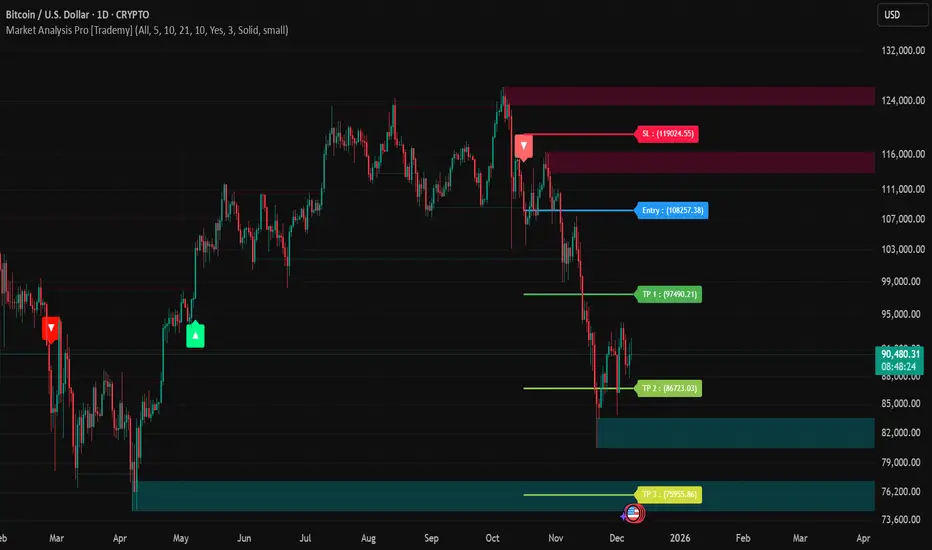
Market Analysis Pro [Trademy]OVERVIEW
Trademy Market Analysis Pro is a professional-grade trading system that combines advanced momentum analysis with institutional-level Supply/Demand zone mapping. This indicator is designed to provide crystal-clear market analysis with precise risk management tools, creating a complete trading framework within a single, streamlined interface.
Unlike complex indicators that overwhelm traders with information, Trademy focuses on what matters: high-probability setups with clear entry points, defined risk levels, and multiple profit targets. The system is built to eliminate guesswork and provide actionable signals that work across multiple timeframes and asset classes eg: ( INDEX:BTCUSD , NASDAQ:NVDA and more )
CORE CONCEPTS
Advanced Momentum Engine: The foundation of Trademy Market Analysis Pro is a proprietary momentum detection system that identifies true directional shifts in the market. The algorithm analyzes price behavior relative to volatility-adjusted dynamic levels, generating signals only when genuine momentum reversals occur. The "Signal Sensitivity" control allows you to adapt the system from conservative (fewer, higher-quality signals) to aggressive (more frequent opportunities) based on your trading style and market conditions.
Institutional Supply/Demand Zones: The system automatically identifies and plots key institutional levels where significant buying (Demand) or selling (Supply) pressure has occurred. These zones are calculated using advanced price structure analysis, filtered through intelligent overlap detection to ensure only the most relevant zones appear on your chart. When price approaches these levels, they often act as strong support or resistance, providing logical areas for entries and exits.
Intelligent Signal Classification: Not all signals are created equal. Trademy categorizes every signal as either "Normal" or "Strong" based on its alignment with the broader market structure and trend context. Strong signals represent higher-conviction setups where momentum and trend align perfectly, while normal signals indicate counter-trend or early reversal opportunities.
Non-Repainting Architecture: Every signal is locked in at bar close (when enabled), and all TP/SL levels are calculated using volatility measurements captured at the moment of signal generation.
KEY FEATURES
Precision Signal System
Dual Signal Modes: Choose between Normal signals (standard momentum reversals) or Strong signals (high-conviction trend-aligned setups), or view both simultaneously
Wait for Bar Close: Optional no-repaint mode ensures signals only appear after candle confirmation
Visual Signal Hierarchy: Normal signals shown with standard arrows (▲/▼), Strong signals marked with distinctive colors for instant recognition
Adjustable Arrow Sizes: Customize signal display from tiny to large based on your chart preferences
Professional Risk Management
Automated TP/SL Calculation: Three take-profit levels (TP1, TP2, TP3) and one stop-loss level automatically calculated using advanced volatility measurement
Fixed Risk Levels: TP/SL lines are locked at signal generation and never move—providing consistent, reliable risk parameters
Visual Risk Zones: Optional colored zones highlight your risk and reward areas for instant position assessment
Adjustable Risk Multiplier: Scale your targets up or down with a single parameter while maintaining proper risk-reward ratios
Clear On-Chart Labels: Every level displays exact price values in an easy-to-read format
Supply/Demand Zone Mapping
Automatic Zone Detection: System identifies high-probability supply and demand zones using advanced price structure analysis
Anti-Overlap Algorithm: Intelligent filtering prevents zone clutter by removing overlapping levels
Extended Zone Projection: Zones extend into the future, showing you key levels before price reaches them
Break-of-Structure Tracking: Monitors when zones are broken and removes invalidated levels
Fully Customizable: Adjust zone colors, swing length, history depth, and box width to match your analysis style
Visual Customization
Flexible Color Schemes: Customize colors for bull/bear signals, TP/SL levels, and supply/demand zones
Trend Background: Optional background coloring to instantly visualize the current market bias
Support/Resistance Lines: Toggle automatic S/R level plotting from key price pivots
Multiple Arrow Sizes: Choose from tiny, small, normal, or large signal arrows
WHAT MAKES TRADEMY MARKET ANALYSIS PRO DIFFERENT
✅ Simplicity Meets Power
✅ TP/SL Levels
✅ Institutional Zone Integration
✅ Universal Indicator for all markets
✅ Multi-Timeframe Flexibility
BEST PRACTICES
📌 Always Use Stop-Loss: Enable the TP/SL system and respect your stop-loss levels,risk management is key to long-term success
📌 Backtest First: Before live trading, replay historical charts to understand signal behavior on your specific asset and timeframe
📌 Combine Timeframes: Use higher timeframe signals as your bias, enter on lower timeframe signals in the same direction
📌 Watch the Zones: Highest probability setups occur when signals align with supply/demand zones (buy near demand, sell near supply)
📌 Don't Chase: If you miss a signal, wait for the next one,forcing trades leads to losses
📌 Partial Profits: Consider taking partial profits at TP1, moving stop to breakeven, and letting the rest run to TP2/TP3
📩 ACCESS & SUPPORT
This is an invite-only indicator. For access inquiries, please contact via TradingView private message.
Important Disclaimers:
This indicator is a tool for technical analysis and does not constitute financial advice
Past performance does not guarantee future results
Always practice proper risk management and never risk more than you can afford to lose
Trading carries substantial risk of loss and is not suitable for all investors
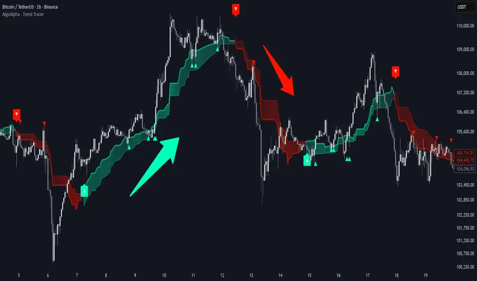
Trend Tracer [AlgoAlpha]🟠 OVERVIEW
This tool builds a two-stage trend model that reacts to structure shifts while also showing how strong or weak the move is. It uses a mid-price band (from the highest high and lowest low over a lookback) and applies two Supertrend passes on top of it. The first pass smoothens the basis. The second pass refines that direction and produces the final trail used for signals. A gradient fill between the two trails uses RSI of price-to-trail distance to show when price is stretched or cooling off. The aim is to give traders a simple way to read trend alignment, pressure, and early turns without guessing.
🟠 CONCEPTS
The script starts with a mid-range basis. This is the average of the rolling highest high and lowest low. It acts as a stable structure reference instead of raw close or typical price. From there, two Supertrend layers are applied:
• The first Supertrend uses a shorter ATR period and lower factor. It reacts faster and sets the main regime.
• The second Supertrend uses a slightly longer ATR and higher factor. It filters noise, waits for confirmed continuation, and generates the signal line.
The interaction between these trails matters. The outer Supertrend provides context by defining the broader regime. The inner Supertrend provides timing by flipping earlier and marking possible shifts. The gradient fill uses RSI of (close − supertrend value) to display when price stretches away from the trail. This shows strength, exhaustion, or compression within the trend.
🟠 FEATURES
Bullish and bearish flip markers placed at recent highs/lows
Rejection signals off the trend tracer line
Alerts for bullish and bearish trend changes
🟠 USAGE
Setup : Add the script to your chart. Timeframe is flexible; lower timeframes show more flips while higher ones give cleaner swings. Adjust Length to change how wide the basis range is. Use the two ATR settings and factors to match the volatility of the market you trade.
Read the chart : When the refined trail (stv_) sits above price the regime is bearish; when below, it is bullish. The wide trail (stv) confirms the larger move. Watch the gradient fill: darker colors appear when price is stretched from the trail and lighter colors appear when the move is weakening. Flip markers ▲ or ▼ highlight the first clean shift of the refined trail.
Settings that matter : Increasing the Main Factor slows main-trend flips and filters chop. Increasing the Signal Factor delays the timing trail but reduces noise. Shortening Length makes the basis more reactive. ATR periods change how sensitive each Supertrend pass is to volatility.
Trend Step Channel [BigBeluga]🔵 OVERVIEW
Trend Step Channel identifies directional bias by forming a dynamic volatility-based step channel. It detects trend shifts when candle lows close above the upper band (bullish) or when candle highs drop below the lower band (bearish). A step-style midline tracks the trend evolution, while an integrated dashboard shows price positioning percentages across multiple timeframes.
🔵 CONCEPTS
ATR-Based Channel — The indicator constructs upper and lower channel boundaries using ATR distance around a single adaptive trend line, providing automatic scaling with volatility.
Trend Direction Logic —
• Low above upper band → uptrend confirmation.
• High below lower band → downtrend confirmation.
Step Trend Line — A reactive midline that locks onto price swings, stepping upward or downward as new trend confirmations occur.
Channel Width — Defines the total volatility range around the midline; a wider channel smooths market noise, while a narrower one reacts faster.
Price Position Ratio — Calculates the relative position of the close within the channel, from 0% (bottom) to 100% (top).
🔵 FEATURES
Volatility-Adaptive Channel — Expands and contracts dynamically to match market volatility, maintaining consistent distance scaling.
Configurable MA Source — Choose from SMA, EMA, SMMA, WMA, or VWMA as the base smoothing method.
Color-Coded Step Line —
• Green indicates an uptrend.
• Orange indicates a downtrend.
Channel Fill Visualization — Semi-transparent fills highlight active volatility zones for clear trend identification.
Price Position Label — Displays a “<” marker and percentage at the channel edge showing how far the current close is from the lower or upper band.
Multi-Timeframe Dashboard —
• Displays alignment across 1H–5H charts.
• Each cell shows an arrow (↑ / ↓) with price % positioning.
• Cell background color reflects bullish or bearish bias.
Real-Time Updating — The channel, midline, and dashboard refresh dynamically every bar for continuous feedback.
🔵 HOW TO USE
Trend Confirmation —
• Bullish trend forms when candle low closes above the upper band.
• Bearish trend forms when candle high closes below the lower band.
Trend Continuation — Maintain bias while the step line color remains consistent.
Volatility Breakouts — Sudden candle breaks outside the band suggest new directional strength.
Dashboard Alignment — Confirm trend consistency across multiple timeframes before entering trades.
Entry Planning — In uptrends, consider entries near the lower band; in downtrends, focus on upper-band rejections.
Price Position Insight — Use the % label to judge whether price is extended (near 100%) or compressed (near 0%) within the channel.
🔵 CONCLUSION
Trend Step Channel delivers a precise, volatility-driven view of trend structure using ATR-based boundaries and a step-line framework. The integrated dashboard, color-coded channel, and live positioning metrics give traders a complete picture of market direction, trend strength, and price location within evolving conditions.

SMC Statistical Liquidity Walls [PhenLabs]📊 SMC Statistical Liquidity Walls
Version: PineScript™ v6
📌 Description
The SMC Statistical Liquidity Walls indicator is designed to visualize market volatility and potential reversal zones using advanced statistical modeling. Unlike traditional Bollinger Bands that use simple lines, this script utilizes an “Inverted Sigmoid” opacity function to create a “fog of war” effect. This visualizes the density of liquidity: the further price moves from the equilibrium (mean), the “harder” the liquidity wall becomes.
This tool solves the problem of over-trading in low-probability areas. By automatically mapping “Premium” (Resistance) and “Discount” (Support) zones based on Standard Deviation (SD), traders can instantly see when price is overextended. The result is a clean, intuitive overlay that helps you identify high-probability mean reversion setups without cluttering your chart with manual drawings.
🚀 Points of Innovation
Inverted Sigmoid Logic: A custom mathematical function maps Standard Deviation to opacity, creating a realistic “wall” density effect rather than linear gradients.
Dynamic “Solidity”: The indicator is transparent at the center (Equilibrium) and becomes visually solid at the edges, mimicking physical resistance.
Separated Directional Bias: distinct Red (Premium) and Green (Discount) coding helps SMC traders instantly recognize expensive vs. cheap pricing.
Smart “Safe” Deviation: Includes fallback logic to handle calculation errors if deviation hits zero, ensuring the indicator never crashes during data gaps.
🔧 Core Components
Basis Calculation: Uses a Simple Moving Average (SMA) to determine the market’s equilibrium point.
Standard Deviation Zones: Calculates 1SD, 2SD, and 3SD levels to define the statistical extremes of price action.
Sigmoid Alpha Calculation: Converts the SD distance into a transparency value (0-100) to drive the visual gradient.
🔥 Key Features
Automated Premium/Discount Zones: Red zones indicate overbought (Premium) areas; Green zones indicate oversold (Discount) areas.
Customizable Density: Users can adjust the “Steepness” and “Midpoint” of the sigmoid curve to control how fast the walls become solid.
Integrated Alerts: Built-in alert conditions trigger when price hits the “Solid” wall (2SD or higher), perfect for automated trading or notifications.
Visual Clarity: The center of the chart remains clear (high transparency) to keep focus on price action where it matters most.
🎨 Visualization
Equilibrium Line: A gray line representing the mean price.
Gradient Fills: The space between bands fills with color that increases in opacity as it moves outward.
Premium Wall: Upper zones fade from transparent red to solid red.
Discount Wall: Lower zones fade from transparent green to solid green.
📖 Usage Guidelines
Range Period: Default 20. Controls the lookback period for the SMA and Standard Deviation calculation.
Source: Default Close. The price data used for calculations.
Center Transparency: Default 100 (Clear). Controls how transparent the middle of the chart is.
Edge Transparency: Default 45 (Solid). Controls the opacity of the outermost liquidity wall.
Wall Steepness: Default 2.5. Adjusts how aggressively the gradient transitions from clear to solid.
Wall Start Point: Default 1.5 SD. The deviation level where the gradient shift begins to accelerate.
✅ Best Use Cases
Mean Reversion Trading: Enter trades when price hits the solid 2SD or 3SD wall and shows rejection wicks.
Take Profit Targets: Use the Equilibrium (Gray Line) as a logical first target for reversal trades.
Trend Filtering: Do not initiate new long positions when price is deep inside the Red (Premium) wall.
⚠️ Limitations
Lagging Nature: As a statistical tool based on Moving Averages, the walls react to past price data and may lag during sudden volatility spikes.
Trending Markets: In strong parabolic trends, price can “ride” the bands for extended periods; mean reversion should be used with caution in these conditions.
💡 What Makes This Unique
Physics-Based Visualization: We treat liquidity as a physical barrier that gets denser the deeper you push, rather than just a static line on a chart.
🔬 How It Works
Step 1: The script calculates the mean (SMA) and the Standard Deviation (SD) of the source price.
Step 2: It defines three zones above and below the mean (1SD, 2SD, 3SD).
Step 3: The custom `get_inverted_sigmoid` function calculates an Alpha (transparency) value based on the SD distance.
Step 4: Plot fills are colored dynamically, creating a seamless gradient that hardens at the extremes to visualize the “Liquidity Wall.”
💡 Note
For best results, combine this indicator with Price Action confirmation (such as pin bars or engulfing candles) when price touches the solid walls.

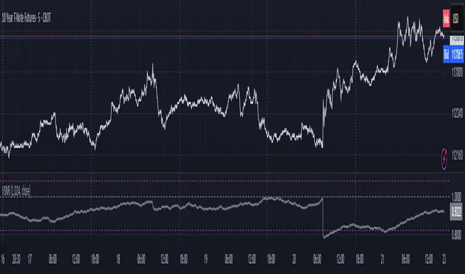
Volatility Signal-to-Noise Ratio🙏🏻 this is VSNR: the most effective and simple volatility regime detector & automatic volatility threshold scaler that somehow no1 ever talks about.
This is simply an inverse of the coefficient of variation of absolute returns, but properly constructed taking into account temporal information, and made online via recursive math with algocomplexity O(1) both in expanding and moving windows modes.
How do the available alternatives differ (while some’re just worse)?
Mainstream quant stat tests like Durbin-Watson, Dickey-Fuller etc: default implementations are ALL not time aware. They measure different kinds of regime, which is less (if at all) relevant for actual trading context. Mix of different math, high algocomplexity.
The closest one is MMI by financialhacker, but his approach is also not time aware, and has a higher algocomplexity anyways. Best alternative to mine, but pls modify it to use a time-weighted median.
Fractal dimension & its derivatives by John Ehlers: again not time aware, very low info gain, relies on bar sizes (high and lows), which don’t always exist unlike changes between datapoints. But it’s a geometric tool in essence, so this is fundamental. Let it watch your back if you already use it.
Hurst exponent: much higher algocomplexity, mix of parametric and non-parametric math inside. An invention, not a math entity. Again, not time aware. Also measures different kinds of regime.
How to set it up:
Given my other tools, I choose length so that it will match the amount of data that your trading method or study uses multiplied by ~ 4-5. E.g if you use some kind of bands to trade volatility and you calculate them over moving window 64, put VSNR on 256.
However it depends mathematically on many things, so for your methods you may instead need multipliers of 1 or ~ 16.
Additionally if you wanna use all data to estimate SNR, put 0 into length input.
How to use for regime detection:
First we define:
MR bias: mean reversion bias meaning volatility shorts would work better, fading levels would work better
Momo bias: momentum bias meaning volatility longs would work better, trading breakouts of levels would work better.
The study plots 3 horizontal thresholds for VSNR, just check its location:
Above upper level: significant Momo bias
Above 1 : Momo bias
Below 1 : MR bias
Below lower level: significant MR bias
Take a look at the screenshots, 2 completely different volatility regimes are spotted by VSNR, while an ADF does not show different regime:
^^ CBOT:ZN1!
^^ INDEX:BTCUSD
How to use as automatic volatility threshold scaler
Copy the code from the script, and use VSNR as a multiplier for your volatility threshold.
E.g you use a regression channel and fade/push upper and lower thresholds which are RMSEs multiples. Inside the code, multiply RMSE by VSNR, now you’re adaptive.
^^ The same logic as when MM bots widen spreads with vola goes wild.
How it works:
Returns follow Laplace distro -> logically abs returns follow exponential distro , cuz laplace = double exponential.
Exponential distro has a natural coefficient of variation = 1 -> signal to noise ratio defined as mean/stdev = 1 as well. The same can be said for Student t distro with parameter v = 4. So 1 is our main threshold.
We can add additional thresholds by discovering SNRs of Student t with v = 3 and v = 5 (+- 1 from baseline v = 4). These have lighter & heavier tails each favoring mean reversion or momentum more. I computed the SNR values you see in the code with mpmath python module, with precision 256 decimals, so you can trust it I put it on my momma.
Then I use exponential smoothing with properly defined alphas (one matches cumulative WMA and another minimizes error with WMA in moving window mode) to estimate SNR of abs returns.
…
Lightweight huh?
∞
Change in State of Delivery CISD [AlgoAlpha]🟠 OVERVIEW
This script tracks how price “changes delivery” after failed attempts to push in one direction. It builds swing levels from pivots, watches for those levels to be wicked, and then checks if price delivers cleanly in the opposite direction. When the pattern meets the script’s tolerance rules, it marks a Change in State of Delivery (CISD). These CISD levels are drawn as origin lines and are used to spot shifts in intent, failed pushes, and continuation attempts. A CISD becomes stronger when it forms after opposing liquidity is swept within a defined lookback.
🟠 CONCEPTS
The script first defines structure using swing highs/lows. These levels act as potential liquidity points. When price wicks through a swing, the script registers a mitigation event. After this, it looks for a reversal-style candle sequence: a failed push, followed by a counter-move strong enough to pass a tolerance ratio. This ratio compares how far price expanded away from the failed attempt versus the counter-move that followed. If the ratio is high enough, this becomes a CISD. The idea is simple: liquidity interaction sets context , and the tolerance logic identifies actual intent . CISD levels and sweep markers combine these two ideas into a clean map of where delivery flipped.
🟠 FEATURES
Liquidity tracking: marks swing highs/lows and updates them until expiry
Liquidity sweep confirmation when CISD aligns with recent mitigations
Alert conditions for all key events: mitigations, CISDs, and strong CISDs
🟠 USAGE
Setup : Add the script to your chart. Use it on any timeframe where swing behavior matters. Set the Swing Period for how wide a pivot must be. Set Noise Filter to control how strict the CISD detection is. Liquidity Lookback defines how recent a wick must be to confirm a sweep.
Read the chart : Origin lines mark where the CISD began. A green line signals bullish intent; a red line signals bearish intent. ▲ and ▼ shapes show CISDs that form after liquidity is swept, these mark strong signals for potential entry. Swing dots show recent swing highs/lows. Candle colors follow the latest CISD trend.
Settings that matter : Increasing Swing Period produces fewer but stronger swings. Raising Noise Filter requires cleaner counter-moves and reduces false CISDs. Liquidity Lookback controls how strict the sweep confirmation is. Expiry Bars decides how long swing levels remain active.

Uptrick: Dynamic Z-Score DivergenceIntroduction
Uptrick: Dynamic Z-Score Divergence is an oscillator that combines multiple momentum sources within a Z-Score framework, allowing for the detection of statistically significant mean-reversion setups, directional shifts, and divergence signals. It integrates a multi-source normalized oscillator, a slope-based signal engine, structured divergence logic, a slope-adaptive EMA with dynamic bands, and a modular bar coloring system. This script is designed to help traders identify statistically stretched conditions, evolving trend dynamics, and classical divergence behavior using a unified statistical approach.
Overview
At its core, this script calculates the Z-Score of three momentum sources—RSI, Stochastic RSI, and MACD—using a user-defined lookback period. These are averaged and smoothed to form the main oscillator line. This normalized oscillator reflects how far short-term momentum deviates from its mean, highlighting statistically extreme areas.
Signals are triggered when the oscillator reverses slope within defined inner zones, indicating a shift in direction while the signal remains in a statistically stretched state. These mean-reversion flips (referred to as TP signals) help identify turning points when price momentum begins to revert from extended zones.
In addition, the script includes a divergence detection engine that compares oscillator pivot points with price pivot points. It confirms regular bullish and bearish divergence by validating spacing between pivots and visualizes both the oscillator-side and chart-side divergences clearly.
A dynamic trend overlay system is included using a Slope Adaptive EMA (SA-EMA). This trend line becomes more responsive when Z-Score deviation increases, allowing the trend line to adapt to market conditions. It is paired with ATR-based bands that are slope-sensitive and selectively visible—offering context for dynamic support and resistance.
The script includes configurable bar coloring logic, allowing users to color candles based on oscillator slope, last confirmed divergence, or the most recent signal of any type. A full alert system is also built-in for key signals.
Originality
The script is based on the well-known concept of Z-Score valuation, which is a standard statistical method for identifying how far a signal deviates from its mean. This foundation—normalizing momentum values such as RSI or MACD to measure relative strength or weakness—is not unique to this script and is widely used in quantitative analysis.
What makes this implementation original is how it expands the Z-Score foundation into a fully featured, signal-producing system. First, it introduces a multi-source composite oscillator by combining three momentum inputs—RSI, Stochastic RSI, and MACD—into a unified Z-Score stream. Second, it builds on that stream with a directional slope logic that identifies turning points inside statistical zones.
The most distinctive additions are the layered features placed on top of this normalized oscillator:
A structured divergence detection engine that compares oscillator pivots with price pivots to validate regular bullish and bearish divergence using precise spacing and timing filters.
A fully integrated slope-adaptive EMA overlay, where the smoothing dynamically adjusts based on real-time Z-Score movement of RSI, allowing the trend line to become more reactive during high-momentum environments and slower during consolidation.
ATR-based dynamic bands that adapt to slope direction and offer real-time visual zones for support and resistance within trend structures.
These features are not typically found in standard Z-Score indicators and collectively provide a unique approach that bridges statistical normalization, structure detection, and adaptive trend modeling within one script.
Features
Z-Score-based oscillator combining RSI, StochRSI, and MACD
Configurable smoothing for stable composite signal output
Buy/Sell TP signals based on slope flips in defined zones
Background highlighting for extreme outer bands
Inner and outer zones with fill logic for statistical context
Pivot-based divergence detection (regular bullish/bearish)
Divergence markers on oscillator and price chart
Slope-Adaptive EMA (SA-EMA) with real-time adaptivity based on RSI Z-Score
ATR-based upper and lower bands around the SA-EMA, visibility tied to slope direction
Configurable bar coloring (oscillator slope, divergence, or most recent signal)
Alerts for TP signals and confirmed divergences
Optional fixed Y-axis scaling for consistent oscillator view
The full setup mode can be seen below:
Input Parameters
General Settings
Full Setup: Enables rendering of the full visual system (lines, bands, signals)
Z-Score Lookback: Lookback period for normalization (mean and standard deviation)
Main Line Smoothing: EMA length applied to the averaged Z-Score
Slope Detection Index: Used to calculate directional flips for signal logic
Enable Background Highlighting: Enables visual region coloring in
overbought/oversold areas
Force Visible Y-Axis Scale: Forces max/min bounds for a consistent oscillator range
Divergence Settings
Enable Divergence Detection: Toggles divergence logic
Pivot Lookback Left / Right: Defines the structure of oscillator pivot points
Minimum / Maximum Bars Between Pivots: Controls the allowed spacing range for divergence validation
Bar Coloring Settings
Bar Coloring Mode:
➜ Line Color: Colors bars based on oscillator slope
➜ Latest Confirmed Signal: Colors bars based on the most recent confirmed divergence
➜ Any Latest Signal: Colors based on the most recent signal (TP or divergence)
SA-EMA Settings
RSI Length: RSI period used to determine adaptivity
Z-Score Length: Lookback for normalizing RSI in adaptive logic
Base EMA Length: Base length for smoothing before adaptivity
Adaptivity Intensity: Scales the smoothing responsiveness based on RSI deviation
Slope Index: Determines slope direction for coloring and band logic
Band ATR Length / Band Multiplier: Controls the width and responsiveness of the trend-following bands
Alerts
The script includes the following alert conditions:
Buy Signal (TP reversal detected in oversold zone)
Sell Signal (TP reversal detected in overbought zone)
Confirmed Bullish Divergence (oscillator HL, price LL)
Confirmed Bearish Divergence (oscillator LH, price HH)
These alerts allow integration into automation systems or signal monitoring setups.
Summary
Uptrick: Dynamic Z-Score Divergence is a statistically grounded trading indicator that merges normalized multi-momentum analysis with real-time slope logic, divergence detection, and adaptive trend overlays. It helps traders identify mean-reversion conditions, divergence structures, and evolving trend zones using a modular system of statistical and structural tools. Its alert system, layered visuals, and flexible input design make it suitable for discretionary traders seeking to combine quantitative momentum logic with structural pattern recognition.
Disclaimer
This script is for educational and informational purposes only. No indicator can guarantee future performance, and trading involves risk. Always use risk management and test strategies in a simulated environment before deploying with live capital.

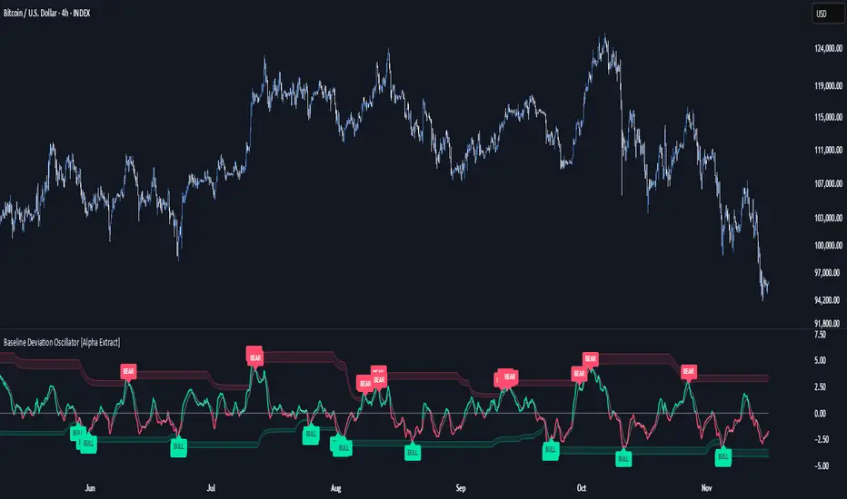
Baseline Deviation Oscillator [Alpha Extract]A sophisticated normalized oscillator system that measures price deviation from a customizable moving average baseline using ATR-based scaling and dynamic threshold adaptation. Utilizing advanced HL median filtering and multi-timeframe threshold calculations, this indicator delivers institutional-grade overbought/oversold detection with automatic zone adjustment based on recent oscillator extremes. The system's flexible baseline architecture supports six different moving average types while maintaining consistent ATR normalization for reliable signal generation across varying market volatility conditions.
🔶 Advanced Baseline Construction Framework
Implements flexible moving average architecture supporting EMA, RMA, SMA, WMA, HMA, and TEMA calculations with configurable source selection for optimal baseline customization. The system applies HL median filtering to the raw baseline for exceptional smoothing and outlier resistance, creating ultra-stable trend reference levels suitable for precise deviation measurement.
// Flexible Baseline MA System
ma(src, length, type) =>
if type == "EMA"
ta.ema(src, length)
else if type == "TEMA"
ema1 = ta.ema(src, length)
ema2 = ta.ema(ema1, length)
ema3 = ta.ema(ema2, length)
3 * ema1 - 3 * ema2 + ema3
// Baseline with HL Median Smoothing
Baseline_Raw = ma(src, MA_Length, MA_Type)
Baseline = hlMedian(Baseline_Raw, HL_Filter_Length)
🔶 ATR Normalization Engine
Features sophisticated ATR-based scaling methodology that normalizes price deviations relative to current volatility conditions, ensuring consistent oscillator readings across different market regimes. The system calculates ATR bands around the baseline and uses half the band width as the normalization factor for volatility-adjusted deviation measurement.
🔶 Dynamic Threshold Adaptation System
Implements intelligent threshold calculation using rolling window analysis of oscillator extremes with configurable smoothing and expansion parameters. The system identifies peak and trough levels over dynamic windows, applies EMA smoothing, and adds expansion factors to create adaptive overbought/oversold zones that adjust to changing market conditions.
1D
3D
1W
🔶 Multi-Source Configuration Architecture
Provides comprehensive source selection including Close, Open, HL2, HLC3, and OHLC4 options for baseline calculation, enabling traders to optimize oscillator behavior for specific trading styles. The flexible source system allows adaptation to different market characteristics while maintaining consistent ATR normalization methodology.
🔶 Signal Generation Framework
Generates bounce signals when oscillator crosses back through dynamic thresholds and zero-line crossover signals for trend confirmation. The system identifies both standard threshold bounces and extreme zone bounces with distinct alert conditions for comprehensive reversal and continuation pattern detection.
Bull_Bounce = ta.crossover(OSC, -Active_Lower) or
ta.crossover(OSC, -Active_Lower_Extreme)
Bear_Bounce = ta.crossunder(OSC, Active_Upper) or
ta.crossunder(OSC, Active_Upper_Extreme)
// Zero Line Signals
Zero_Cross_Up = ta.crossover(OSC, 0)
Zero_Cross_Down = ta.crossunder(OSC, 0)
🔶 Enhanced Visual Architecture
Provides color-coded oscillator line with bullish/bearish dynamic coloring, signal line overlay for trend confirmation, and optional cloud fills between oscillator and signal. The system includes gradient zone fills for overbought/oversold regions with configurable transparency and threshold level visualization with automatic label generation.
snapshot
🔶 HL Median Filter Integration
Features advanced high-low median filtering identical to DEMA Flow for exceptional baseline smoothing without lag introduction. The system constructs rolling windows of baseline values, performs median extraction for both odd and even window lengths, and eliminates outliers for ultra-clean deviation measurement baseline.
🔶 Comprehensive Alert System
Implements multi-tier alert framework covering bullish bounces from oversold zones, bearish bounces from overbought zones, and zero-line crossovers in both directions. The system provides real-time notifications for critical oscillator events with customizable message templates for automated trading integration.
🔶 Performance Optimization Framework
Utilizes efficient calculation methods with optimized array management for median filtering and minimal computational overhead for real-time oscillator updates. The system includes intelligent null value handling and automatic scale factor protection to prevent division errors during extreme market conditions.
🔶 Why Choose Baseline Deviation Oscillator ?
This indicator delivers sophisticated normalized oscillator analysis through flexible baseline architecture and dynamic threshold adaptation. Unlike traditional oscillators with fixed levels, the BDO automatically adjusts overbought/oversold zones based on recent oscillator behavior while maintaining consistent ATR normalization for reliable cross-market and cross-timeframe comparison. The system's combination of multiple MA type support, HL median filtering, and intelligent zone expansion makes it essential for traders seeking adaptive momentum analysis with reduced false signals and comprehensive reversal detection across cryptocurrency, forex, and equity markets.
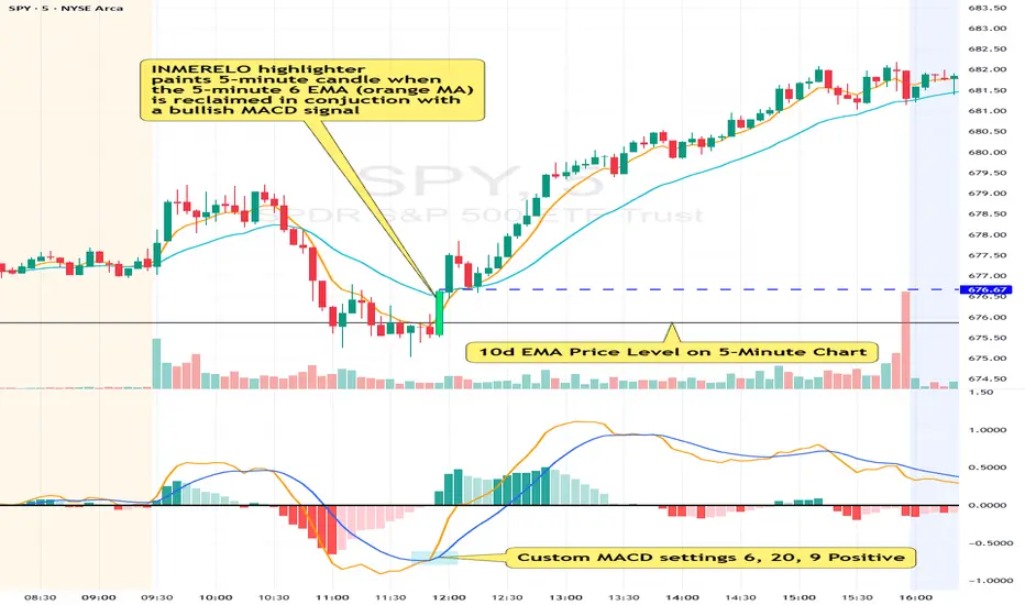
INMERELO EMA Reclaim HighlighterOverview
The INMERELO EMA Reclaim indicator highlights intraday candles reclaiming a configurable EMA on any timeframe. It identifies candles based on customizable candle geometry filters and confirms momentum using a custom MACD setup.
Features
Configurable Intraday EMA
Any EMA length and timeframe. Default: 6-period EMA on chart timeframe.
Highlights when price reclaims the EMA after a configurable number of prior closes below it.
Candle Geometry Filters (ORB-Style)
Open Position: Maximum position of open relative to candle range (0–1). Default: 0.40
Close Position: Minimum position of close relative to candle range (0–1). Default: 0.70
Body Fraction: Minimum body size relative to candle range. Default: 0.50
Custom MACD Filter
Fast line above slow line.
Configurable: Fast (default 6), Slow (default 20), Signal (default 9).
Prior Closes Below EMA Filter
Configurable minimum number of prior closes below EMA. Default: 2
Visual Options
Paint candle with configurable color.
Optional arrow display above reclaim candle (toggleable).
Flexible
Works on any intraday timeframe, including 5-minute, 2-minute, 15-minute, etc.
Settings Overview
Setting Default Notes
EMA Length 6 EMA used for reclaim detection
EMA Timeframe Chart TF Can be set to any intraday timeframe
Open ≤ 0.40 ORB-style filter
Close ≥ 0.70 ORB-style filter
Body Fraction 0.50 ORB-style filter
Min Prior Closes Below EMA 2 Minimum closes below EMA before reclaim
MACD Fast 6 Custom MACD fast line
MACD Slow 20 Custom MACD slow line
MACD Signal 9 Custom MACD signal line
Paint Candle True Highlights valid candles
Candle Color Lime Configurable
Show Arrow False Optional visual
Summary:
The INMERELO EMA Reclaim indicator identifies intraday candles reclaiming a configurable EMA, filtered by customizable candle geometry and MACD momentum. Visual options include painted candles and optional arrows, and all settings are fully configurable.
Market Extreme Zones IndexThe Market Extreme Zones Index is a new mean reversion (valuation) tool focused on catching long term oversold/overbought zones. Combining an enhanced RSI with a smoothed Z-score this indicator allows traders to find oppurtunities during highly oversold/overbought zones.
I will separate the explanation into the following parts:
1. How does it work?
2. Methodologies & Concepts
3. Use cases
How does it work?
The indicator attempts to catch highly unprobable events in either direction to capture reversal points over the long term. This is done by calculating the Z-Score of an enhanced RSI.
First we need to calculate the Enhanced RSI:
For this we need to calculate 2 additional lengths:
Length1 = user defined length
Length2 = Length1/2
Length3 = √Length
Now we need to calculate 3 different RSIs:
1st RSI => uses classic user defined source and classic user defined length.
2nd RSI => uses classic user defined source and Length 2.
3rd RSI => uses RSI 2 as source and Length 2
Now calculate the divergence:
RSI_base => 2nd RSI * 3 - 1st RSI - 3rd RSI
After this we need to calculate the median of the RSI_base over √Length and make a divergence of these 2:
RSI => RSI_base*2 - median
All that remains now is the Z-score calculations:
We need:
Average RSI value
Standard Deviation = a measure of how dispersed or spread out a set of data values are from their average
Z-score = (Current Value - Average Value) / Standard Deviation
After this we just smooth the Z-score with a Weighted Moving average with √Length
Methodology & Concepts
Mean Reversion Methodology:
The methodology behind mean reversion is the theory that asset prices will eventually return to their long-term average after deviating significantly, driven by the belief that extreme moves are temporary.
Z-Score Methodology:
A Z-score, or standard score, is a statistical measure that indicates how many standard deviations a data point is from the mean of a dataset. A positive z-score means the value is above the mean, a negative score means it's below, and a score of zero means the value is equal to the mean.
You might already be able to see where I am going with this:
Z-Score could be used for the extreme moves to capture reversal points.
By applying it to the RSI rather than the Price, we get a more accurate measurement that allow us to get a banger indicator.
Use Cases
Capturing reversal points
Trend Direction
- while the main use it for mean reversion, the values can indicate whether we are in an uptrend or a downtrend.
Advantages:
Visualization:
The indicator has many plots to ensure users can easily see what the indicator signals, such as highlighting extreme conditions with background colors.
Versatility:
This indicator works across multiple assets, including the S&P500 and more, so it is not only for crypto.
Final note:
No indicator alone is perfect.
Backtests are not indicative of future performance.
Hope you enjoy Gs!
Good luck!

Screener (ILPAC) [AlgoAlpha]🟠 OVERVIEW
This script is a powerful multi-symbol scanner designed to work as a companion to the "Institutional Liquidity & PA Concepts" (ILPAC) indicator. It allows you to monitor the key price action and liquidity signals from the ILPAC suite across a watchlist of up to 18 assets, all from a single dashboard. The primary goal of this tool is to provide a high-level market overview, enabling you to efficiently spot assets that are showing strong structural trends, interacting with key liquidity zones, or exhibiting signs of FOMO-driven volatility.
Instead of switching between dozens of charts, you can use this screener to quickly filter for assets that meet your specific trading criteria based on the advanced concepts of market structure, liquidity analysis, trend lines, and market sentiment.
🟠 CONCEPTS
The screener is built upon the core analytical engine of the "Institutional Liquidity & PA Concepts" indicator. It applies the proprietary algorithms of the ILPAC indicator to each symbol in your watchlist and presents the results in an easy-to-digest table. The concepts are combined to create a holistic view of the market.
Each column in the table is a window into a specific trading concept:
Market Structure: This is the foundation of price action analysis. The screener identifies the current market trend (bullish or bearish) by tracking swing highs and lows. It also flags critical events like a Break of Structure (BOS), which signals trend continuation, and a Change of Character (CHoCH), which suggests a potential trend reversal.
Liquidity Analysis: The screener analyzes order flow to determine where significant liquidity is resting. The "Liquidity Bias" column shows the net direction of this pressure, while the "Liquidity Event" column alerts you when price interacts with these key zones, either by forming a new one or mitigating an old one.
Trend Lines: This concept automates the classic technical analysis technique of drawing trend lines. The screener identifies significant swing points to form trend lines and then monitors them, alerting you to potential trend continuations or breakouts.
FOMO Bubbles: This concept measures crowd psychology by identifying sudden spikes in volume and price movement that are characteristic of "Fear of Missing Out." These signals can help identify potential trend exhaustion points or the start of a speculative rally.
By presenting these distinct but interconnected concepts together, the screener provides a multi-faceted view that allows traders to build a strong, confluence-based trading thesis.
🟠 FEATURES
This screener organizes a vast amount of data into a simple, color-coded table. Here is a breakdown of each column and the values you can expect to see:
Asset: Displays the ticker symbol for the asset being analyzed.
Market Structure: Shows the dominant trend based on swing highs and lows.
Bull: The asset is in a structural uptrend (making higher highs and higher lows).
Bear: The asset is in a structural downtrend (making lower highs and lower lows).
Detecting: The trend is neutral or a clear structure has not yet been established.
Structure Event: Flags the most recent significant market structure event.
Bull CHoCH: A bullish Change of Character, signaling a potential shift from a downtrend to an uptrend.
Bear CHoCH: A bearish Change of Character, signaling a potential shift from an uptrend to a downtrend.
Bull BOS: A bullish Break of Structure, confirming the continuation of an uptrend.
Bear BOS: A bearish Break of Structure, confirming the continuation of a downtrend.
–: No significant event has occurred recently.
Latest Swing Label: Identifies the most recently confirmed swing point.
HH: Higher High.
HL: Higher Low.
LH: Lower High.
LL: Lower Low.
–: No new swing point has been confirmed.
Liquidity Bias: Measures the net direction of liquidity and its relative strength.
▲ : A bullish liquidity bias, where the number indicates the strength.
▼ : A bearish liquidity bias, where the number indicates the strength.
Balanced: Liquidity is relatively balanced between buyers and sellers.
Liquidity Event: Indicates recent interactions with key liquidity zones.
New▲: A new bullish liquidity zone has just formed.
New▼: A new bearish liquidity zone has just formed.
Mit▲: Price has just tested (mitigated) a key bullish liquidity zone.
Mit▼: Price has just tested (mitigated) a key bearish liquidity zone.
–: No recent interaction.
Trend Line: Displays the status of automatically drawn trend lines.
Break▲: Price has broken above a key bearish trend line.
Break▼: Price has broken below a key bullish trend line.
Bull TL: Price is respecting an active bullish trend line.
Bear TL: Price is respecting an active bearish trend line.
–: No significant trend line is currently active.
FOMO: Detects sentiment-driven price moves of varying intensity.
Big▲/Med▲/Small▲: A bullish FOMO bubble has been detected (large, medium, or small).
Big▼/Med▼/Small▼: A bearish FOMO bubble has been detected (large, medium, or small).
–: No FOMO activity detected.
🟠 USAGE
The primary way to use this screener is to quickly scan your watchlist for assets that exhibit a confluence of bullish or bearish signals, which can significantly improve the probability of a trade.
1. Setup and Configuration:
Add the screener to your chart.
Open the settings and populate the "Watchlist" section with the symbols you want to track.
Fine-tune the input settings for each component (Market Structure, Liquidity, etc.) to match your preferred trading style. These settings will apply to all symbols in the table.
2. Interpreting the Columns for Trading Decisions:
Market Structure Columns: Use the first three structure columns to define your trading bias. For a high-probability long setup, you would look for an asset with a "Bull" structure, a recent "Bull BOS" event, and a "HL" as the latest swing point. This confirms the uptrend is healthy and ongoing.
Liquidity Columns: These are crucial for identifying key price levels. A strong "Liquidity Bias" can confirm your directional bias. A "Mit▲" (mitigation) event at a support level can be a powerful entry trigger, as it shows that institutional buy orders are defending that zone.
Trend Line Column: This is ideal for breakout traders. A "Break▲" signal can serve as an excellent entry confirmation, especially if the overall "Market Structure" is already "Bull".
FOMO Column: This column is best used for identifying potential exhaustion points. For instance, if you are in a long trade and a "Big▲" FOMO signal appears after a strong rally, it could be a sign that the move is overextended and it's a good time to consider taking profits.
Ücretli komut dosyası

Screener (MC) [AlgoAlpha]🟠 OVERVIEW
This script is a multi-symbol scanner that works as a companion to the "Momentum Concepts" indicator. It provides a comprehensive dashboard view, allowing traders to monitor the momentum signals of up to 18 different assets in real-time from a single chart. The main purpose is to offer a bird's-eye view of the market, helping you quickly identify assets with strong momentum confluence or potential reversal opportunities without having to switch between different charts.
The screener displays the status of all key components from the Momentum Concepts indicator, including the Fast Oscillator, Scalper's Momentum, Momentum Impulse Oscillator, and Hidden Liquidity Flow, organizing them into a clear and easy-to-read table.
🟠 CONCEPTS
The core of this screener is built upon the analytical framework of the "Momentum Concepts" indicator, which evaluates market momentum across multiple layers: short-term, medium-term, and long-term. This screener applies those complex, proprietary calculations to each symbol in your watchlist and visualizes the current state of each component.
Each column in the table represents a specific aspect of momentum analysis:
Fast Oscillator Columns: These columns reflect the short-term momentum. They show the immediate trend direction, whether the asset is in an overbought or oversold condition, and flag high-probability events like divergences, reversals, or diminishing momentum.
Scalper's Momentum Column: This column gives insight into medium-term momentum. It distinguishes between strong, sustained moves and weakening, corrective moves, which is useful for gauging the health of a trend.
Momentum Impulse Column: This column represents the dominant, long-term trend bias. It helps you understand the underlying market regime (bullish, bearish, or consolidating) to align your trades with the bigger picture.
Hidden Liquidity Flow Column: This column provides a unique view into the market's underlying liquidity dynamics. It signals whether there is net buying or selling pressure and uses special coloring to highlight periods of unusually high liquidity activity, which often precedes volatile price movements.
By combining these perspectives, the screener justifies its utility by enabling traders to make more informed decisions based on multi-layered signal confluence.
🟠 FEATURES
This screener organizes momentum data into several key columns. Here is a breakdown of each column and its possible values:
Asset: Displays the symbol for the asset being analyzed in that row.
Fast Oscillator Trend: Shows the immediate, short-term momentum direction.
▲: Indicates a bullish short-term trend.
▼: Indicates a bearish short-term trend.
–: Indicates a neutral or transitional state.
Fast Oscillator Valuation: Measures whether the asset is in a short-term overbought or oversold state.
OB: Signals an "Overbought" condition, often associated with bullish exhaustion.
OS: Signals an "Oversold" condition, often associated with bearish exhaustion.
Neutral: The asset is trading in a neutral zone, neither overbought nor oversold.
Scalper's Momentum: Assesses the strength and direction of medium-term momentum.
Strong▲: Strong bullish momentum.
Weak▲: Bullish momentum exists but is weakening or corrective.
Strong▼: Strong bearish momentum.
Weak▼: Bearish momentum exists but is weakening or corrective.
–: Neutral or no clear medium-term momentum.
Momentum Impulse: Identifies the dominant, long-term trend bias. A colored background indicates that the momentum is in a strong "impulse" phase.
▲: Indicates a bullish long-term bias.
▼: Indicates a bearish long-term bias.
0: Indicates a neutral or ranging market condition.
Hidden Liquidity Flow: Tracks underlying buying and selling pressure. The background color highlights periods of unusual liquidity activity.
▲: Positive liquidity flow, suggesting net buying pressure.
▼: Negative liquidity flow, suggesting net selling pressure.
–: Neutral liquidity flow.
Dim. Momentum: Provides an early warning that short-term momentum is beginning to fade.
● (Bullish Color): Bullish momentum is weakening.
● (Bearish Color): Bearish momentum is weakening.
–: No diminishing momentum detected.
Divergence: Flags classic or hidden divergences between price and the Fast Oscillator.
Div▲: A bullish divergence has been detected.
Div▼: A bearish divergence has been detected.
–: No active divergence signal.
Reversal: Signals a potential reversal when the Fast Oscillator crosses its trend line from an overbought or oversold zone.
Rev▲: A bullish reversal signal has occurred.
Rev▼: A bearish reversal signal has occurred.
–: No active reversal signal.
🟠 USAGE
The primary function of this screener is to quickly identify trading opportunities and filter setups based on momentum confluence across your watchlist.
1. Setup and Configuration:
Add the indicator to your chart.
Go into the script settings and populate the "Watchlist" group with the symbols you wish to monitor.
Adjust the settings for the various momentum components (Fast Oscillator, Scalper's Momentum, etc.) to align with your trading strategy. These settings will be universally applied to all symbols in the screener.
2. Interpreting the Columns for Trading Decisions:
Momentum Impulse & Hidden Liquidity Flow: Use these columns to establish a directional bias. A bullish "▲" in both columns on an asset suggests a strong underlying uptrend with supportive buying pressure, making it a good candidate for long positions.
Scalper's Momentum: Use this for entry timing and trend health. A "Strong▲" reading can confirm the strength of an uptrend, while a shift to "Weak▲" might suggest it's time to tighten stops or look for an exit.
Fast Oscillator Trend & Valuation: These are best for precise entry triggers. For a "buy the dip" strategy in an uptrend, you could wait for the Fast Oscillator to show "OS" (Oversold) and then enter when the "Trend" column flips back to "▲".
Dim. Momentum: This is an excellent take-profit signal. If you are in a long position and a bullish-colored "●" appears, it's a warning that the upward move is losing steam, and you might consider closing your trade.
Divergence & Reversal: These columns are for identifying potential turning points. A "Div▲" or "Rev▲" signal is a strong alert that a downtrend might be ending, making the asset a prime candidate to watch for a long entry.
3. Finding High-Probability Setups:
Trend Confluence: Look for assets where multiple components show alignment. For example, an ideal long setup might show a bullish "Momentum Impulse" (▲), a "Strong▲" reading in "Scalper's Momentum," and a bullish trend in the "Fast Oscillator." This indicates that the long-term, medium-term, and short-term momentums are all in agreement.
Reversal and Exhaustion: Use the "Divergence" and "Reversal" columns to spot potential turning points. A "Div▲" signal appearing in an asset that is in an oversold "Fast Oscillator Valuation" zone can be a strong indication of an upcoming bounce.
Ücretli komut dosyası

Consolidation Value Zones (Recio)Consolidation Value Zones introduces an original algorithm to identify consolidation ranges and locate areas of importance within them. This new method "looks" at the chart and draws zones based on price with the goal of producing actionable zones which appear natural, as if they were found through a human analysis.
> Consider the following...
The chart image above displays Bitcoin, at no specific date, for no specific reason. What I have done here is simply glanced at the chart for about 5 seconds, and circled a few areas which stood out as "obvious" consolidation. It does not take a savant to look at a chart and circle ranging price. However, what we have just done defies many common systems for identifying consolidation. We have located ranges of various zone lengths, as small as roughly 25 bars to as large as roughly 100 bars. Regardless of this, we still determined these zones with our eyes and brain in a few seconds, for some it's practically instant. The issue with us humans doing this, is that we are subjective. We did not really use any concrete rules to determine these areas with our eyes. So the problem becomes "How do we identify these zones in a way which seems natural to us with a repeatable system?" Because of this, my approach is simply a logical attempt to reverse engineer our human intuition.
> Consolidation Value Zones
The name of this indicator is generic. To dissect it, we are identifying consolidation ranges, then using a volume profile to determine the value zone within that range. The specific method used to identify these consolidation zones is something I've personally been referring to as the "skewer" method. Another name that may fit better is "Linear Range Alignment/Overlap".
Ultimately, the goal is to locate a single price level or range that overlaps many adjacent bars.
This should, in theory, return areas of visually obvious consolidation.
> The Skewer Method (Identification Method & Bar Gap Allowances)
One consistent concept across the different identification methods for determining consolidation is time. How long do we chop around before calling it consolidation? This is the "Identification Threshold". Once we have located a consolidation zone "this" wide, we will then consider it as consolidation.
In the chart image above, we are considering a six-bar consolidation formation. The figure on the left shows an example of a perfect raw bar overlap, we can see that the six bars all overlap at one price range. This is a perfect example of what we are looking to identify as consolidation. Unfortunately, if this was all we looked at, we would have a very scarce identification method.
For that reason, we have the example on the right, which shows the additional allowances for the identification of these ranges. At most, the example on the right shows a gapless three-bar overlap. However, if we allow the identification to bridge across the gaps, we are able to draw a zone directly through the center and still be within our parameters. This allowance is the "Bar Gap Allowance" and will determine the leniency of the identification.
Between our identification threshold and bar gap allowance, we can start to piece together how the script is "looking" at our chart.
> Detecting Consolidation (Live Detection)
To aid in transparency and user understanding, the live detection calculation can be seen on the chart as a box, skewering the recent historical bars with a number next to it, indicating the number of bars found as potential consolidation.
As we can see in the chart image above, the script, by default, is looking for a 15-bar consolidation, with a 5-bar gap allowance. In the image, the specific gap count is labeled, we can see the script scan backwards as far as it can before counting five gaps in the data. Once that occurs, the detection stops.
Notice how the zone found is a range, consisting of all price levels which meet the parameters. The lower level of the range only had two gaps, but the upper level reached five.
> Consolidation Range and Value Zones (Volume Profiles)
Once the script has identified the consolidation formation, it calculates a volume profile across the identified consolidation range. From this it calculates and draws the Point of Control (POC) and Value Area in addition to the full consolidation range.
Once we have our zones drawn, and understand what they identify, we can go one step further and apply concepts from volume profile trading.
Range High/Low: Displays the current extent of the identified consolidation.
Value High/Low: Shows the specific area within the consolidation where buyers and sellers found the most value.
POC: The single point, where the most volume was transacted during consolidation.
In a balanced market, we would anticipate price to rotate around POC, oscillating from Value High (VAH) to Value Low (VAL). In contrast, a market in motion moves directionally, building volume at new price levels as value, naturally the POC shifts with it.
> Zone Extensions
Unlike many other scripts, there is no mitigation logic at play here, since crossing a zone simply tells us "buyers and sellers are not currently active here", but it does not guarantee that value cannot return or react from previous areas of value.
Obviously the current zone will always be most relevant, but historical zones can retain relevance depending on the context of the market.
Remember: Each area of consolidation is an area where buyers and sellers were once facing off, resulting in price's consolidation. Amidst this, the value zone was the area of greatest agreement between the participants at that time. When moving outside of a range, we would typically look at historical value areas and price's interaction with them for further context.
Due to the ever changing market, there is no fixed extension lookback that will cover every scenario. By default, the Extension Lookback is "1", meaning the script will extend the most recent zone forward until a new zone is detected.
Note: For clarity, zone extensions are colored differently from core zones.
The following chart image shows a few examples of these unique interactions.
As seen in the chart image, looking to previous areas of value as well as POC can provide context in the form of acceptance or rejection at these levels, providing further insight into the auction for us to respond to.
The zones do contain logic to maintain a clean display. By default, the zones extend conditionally when price returns to the previous consolidation range. If desired, the zones can be extended regardless of price action; this can be toggled with the option "Regardless Extension Mode", as seen below.
> Hollow Candles & Zone Merging
When consolidation is identified, a hollow candle is drawn; these can be used to see exactly when each zone is identified. It is important to understand that consolidation zones stemming from the same origin are merged into one zone. This is a frequent occurrence when the consolidation threshold is passed, but the consolidation continues. For this reason you will often see multiple hollow candles in the later areas of the zones.
Similarly, zones from different origin points that overlap are also merged into one consolidation zone. This ensures that no core zones overlap.
Additionally, every time a zone is merged, a new volume profile for the area is calculated.
> Bar Gap Allowance Type (Technical Explanation)
The specific bar gap allowance value can be altered, but so can the type of allowance being used. While some analyses may benefit from counting the total amount of bar gaps within the consolidation, others may benefit from detecting based on consecutive bar gaps.
The chart image above displays the gap counts for each gap allowance type.
The total bar gap allowance type will count until the gap amount is reached, then terminate detection once the allowed number of gaps has been exceeded.
The consecutive bar gap allowance type resets its count once it finds a valid bar within range, by doing so, it only counts the bars that separate each island of in-range bars.
Both methods have merit.
> Implementation
This identification method has proven effective to identify consolidation across market types. As a result, there cannot be one configuration of settings to fit every application. Adapting the detection type and method for each trader's specific market conditions is highly recommended.
When determining parameters, it is helpful to consider time, as it plays a major role in the identification method.
On a 1D chart, the default threshold of 15 corresponds to 15 days, or about 3 weeks depending on the ticker. To identify periods of one-week consolidation, a threshold of 5 would be suitable. To detect perfect gapless weeks, a bar gap allowance of 0 could be used, as seen in the chart image below.
Additional Example:
In the chart image above, we see a 15-second forex chart over the span of a few hours. The detection parameters are set up to detect 15-minute consolidation with a 2-minute max dead zone (consecutive bar gap).
> Detection Source
By default, the script detects consolidation ranges using the full extent of candle wicks. While this is traditional, detection can also be done using only the candle bodies. These identifications are much more nuanced, detecting only from confirmed candle price action; they do not trigger at the same frequency as wick detection.
Optionally, a "Wick/Body Average" can be chosen as the source for detection; as the name implies, this uses the average value between the candle body and its respective wick.
> Additional Settings
The settings mentioned thus far serve as core parameters for identifying consolidation. The following parameters are simply included for the benefit of the advanced user. It is not recommended to adjust these settings under normal circumstances.
- Value Area Percent: Default = 68.26, while traditionally 70 for volume profiles, 68.26 is accurate to the values of a standard bell-curve distribution. The differences are minimal in application.
- VP Rows: Default = 99, Sets the number of rows to be used when calculating the Volume Profiles (VP); note that higher values will lead to a slower calculation. Max value: 999
> Final Notes
If you have made it this far, thank you for reading.
I hope you find value in this new consolidation identification system and understand the logic behind it.
That's it.
Ücretli komut dosyası

McMillan Volatility Bands (MVB) – with Entry Logic// McMillan Volatility Bands (MVB) with signal + entry logic
// Author: ChatGPT for OneRyanAlexander
// Notes:
// - Bands are computed using percentage volatility (log returns), per the Black‑Scholes framing.
// - Inner band (default 3σ) and outer band (default 4σ) are configurable.
// - A setup occurs when price closes outside the outer band, then closes back within the inner band.
// The bar that re‑enters is the "signal bar." We then require price to trade beyond the signal bar's
// extreme by a user‑defined cushion (default 0.34 * signal bar range) to confirm entry.
// - Includes alertconditions for both setups and confirmed entries.

Reversals & Pullbacks PRO🚀 Reversals & Pullbacks Pro — Predict Market Turning Points with Precision
Stop chasing trends — start anticipating them.
The Reversals & Pullbacks Pro indicator identifies high-probability reversal and pullback zones before they happen, using advanced mean reversion logic and momentum change signals.
What it does:
✅ Detects major reversals and minor pullbacks in real time
✅ Uses dynamic mean reversion algorithms to spot over-extended price moves
✅ Highlights premium entry zones for counter-trend and trend-reversal setups
✅ Works across many markets — Designed for Forex and Indices but can be used on Crypto
✅ Clean visuals with smart alerts (no repainting after candle close)
💡 Perfect for:
Swing traders, scalpers, and day traders who want to catch price turning points before everyone else.
⏱️ Don’t react — predict.
Upgrade your trading with Reversals & Pullback Pro and trade market reversals like a PRO!

Ornstein-Uhlenbeck Trend Channel [BOSWaves]Ornstein-Uhlenbeck Trend Channel - Adaptive Mean Reversion with Dynamic Equilibrium Geometry
Overview
The Ornstein-Uhlenbeck Trend Channel introduces an advanced equilibrium-mapping framework that blends statistical mean reversion with adaptive trend geometry. Traditional channels and regression bands react linearly to volatility, often failing to capture the natural rhythm of price equilibrium. This model evolves that concept through a dynamic reversion engine, where equilibrium adapts continuously to volatility, trend slope, and structural bias - forming a living channel that bends, expands, and contracts in real time.
The result is a smooth, equilibrium-driven representation of market balance - not just trend direction. Instead of static bands or abrupt slope shifts, traders see fluid, volatility-aware motion that mirrors the natural pull-and-release dynamic of market behavior. Each channel visualizes the probabilistic boundaries of fair value, showing where price tends to revert and where it accelerates away from its statistical mean.
Unlike conventional envelopes or Bollinger-type constructs, the Ornstein-Uhlenbeck framework is volatility-reactive and equilibrium-sensitive, providing traders with a contextual map of where price is likely to stabilize, extend, or exhaust.
Theoretical Foundation
The Ornstein-Uhlenbeck Trend Channel is inspired by stochastic mean-reversion processes - mathematical models used to describe systems that oscillate around a drifting equilibrium. While linear regression channels assume constant variance, financial markets operate under variable volatility and shifting equilibrium points. The OU process accounts for this by treating price as a mean-seeking motion governed by volatility and trend persistence.
At its core are three interacting components:
Equilibrium Mean (μ) : Represents the evolving balance point of price, adjusting to directional bias and volatility.
Reversion Rate (θ) : Defines how strongly price is pulled back toward equilibrium after deviation, capturing the self-correcting nature of market structure.
Volatility Coefficient (σ) : Controls how far and how quickly price can diverge from equilibrium before mean reversion pressure increases.
By embedding this stochastic model inside a volatility-adjusted framework, the system accurately scales across different markets and conditions - maintaining meaningful equilibrium geometry across crypto, forex, indices, or commodities. This design gives traders a mathematically grounded yet visually intuitive interpretation of dynamic balance in live market motion.
How It Works
The Ornstein-Uhlenbeck Trend Channel is constructed through a structured multi-stage process that merges stochastic logic with volatility mechanics:
Equilibrium Estimation Core : The indicator begins by identifying the evolving mean using adaptive smoothing influenced by trend direction and volatility. This becomes the live centerline - the statistical anchor around which price naturally oscillates.
Volatility Normalization Layer : ATR or rolling deviation is used to calculate volatility intensity. The output scales the channel width dynamically, ensuring that boundaries reflect current variance rather than static thresholds.
Directional Bias Engine : EMA slope and trend confirmation logic determine whether equilibrium should tilt upward or downward. This creates asymmetrical channel motion that bends with the prevailing trend rather than staying horizontal.
Channel Boundary Construction : Upper and lower bands are plotted at volatility-proportional distances from the mean. These envelopes form the “statistical pressure zones” that indicate where mean reversion or acceleration may occur.
Signal and Lifecycle Control : Channel breaches, mean crossovers, and slope flips mark statistically significant events - exhaustion, continuation, or rebalancing. Older equilibrium zones gradually fade, ensuring a clear, context-aware visual field.
Through these layers, the channel forms a continuously updating equilibrium corridor that adapts in real time - breathing with the market’s volatility and rhythm.
Interpretation
The Ornstein-Uhlenbeck Trend Channel reframes how traders interpret balance and momentum. Instead of viewing price as directional movement alone, it visualizes the constant tension between trending force and equilibrium pull.
Uptrend Phases : The equilibrium mean tilts upward, with price oscillating around or slightly above the midline. Upper band touches signal momentum extension; lower touches reflect healthy reversion.
Downtrend Phases : The mean slopes downward, with upper-band interactions marking resistance zones and lower bands acting as reversion boundaries.
Equilibrium Transitions : Flat mean sections indicate balance or distribution phases. Breaks from these neutral zones often precede directional expansion.
Overextension Events : When price closes beyond an outer boundary, it marks statistically significant disequilibrium - an early warning of exhaustion or volatility reset.
Visually, the OU channel translates volatility and equilibrium into structured geometry, giving traders a statistical lens on trend quality, reversion probability, and volatility stress points.
Strategy Integration
The Ornstein-Uhlenbeck Trend Channel integrates seamlessly into both mean-reversion and trend-continuation systems:
Trend Alignment : Use mean slope direction to confirm higher-timeframe bias before entering continuation setups.
Reversion Entries : Target rejections from outer bands when supported by volume or divergence, capturing snapbacks toward equilibrium.
Volatility Breakout Mapping : Monitor boundary expansions to identify transition from compression to expansion phases.
Liquidity Zone Confirmation : Combine with BOS or order-block indicators to validate structural zones against equilibrium positioning.
Momentum Filtering : Align with oscillators or volume profiles to isolate equilibrium-based pullbacks with statistical context.
Technical Implementation Details
Core Engine : Stochastic Ornstein-Uhlenbeck process for continuous mean recalibration.
Volatility Framework : ATR- and deviation-based scaling for dynamic channel expansion.
Directional Logic : EMA-slope driven bias for adaptive mean tilt.
Channel Composition : Independent upper and lower envelopes with smoothing and transparency control.
Signal Structure : Alerts for mean crossovers and boundary breaches.
Performance Profile : Lightweight, multi-timeframe compatible implementation optimized for real-time responsiveness.
Optimal Application Parameters
Timeframe Guidance:
1 - 5 min : Reactive equilibrium tracking for short-term scalping and microstructure analysis.
15 - 60 min : Medium-range setups for volatility-phase transitions and intraday structure.
4H - Daily : Macro equilibrium mapping for identifying exhaustion, distribution, or reaccumulation zones.
Suggested Configuration:
Mean Length : 20 - 50
Volatility Multiplier : 1.5× - 2.5×
Reversion Sensitivity : 0.4 - 0.8
Smoothing : 2 - 5
Parameter tuning should reflect asset liquidity, volatility, and desired reversion frequency.
Performance Characteristics
High Effectiveness:
Trending environments with cyclical pullbacks and volatility oscillation.
Markets exhibiting consistent equilibrium-return behavior (indices, majors, high-cap crypto).
Reduced Effectiveness:
Low-volatility consolidations with minimal variance.
Random walk markets lacking definable equilibrium anchors.
Integration Guidelines
Confluence Framework : Pair with BOSWaves structural tools or momentum oscillators for context validation.
Directional Control : Follow mean slope alignment for directional conviction before acting on channel extremes.
Risk Calibration : Use outer band violations for controlled contrarian entries or trailing stop management.
Multi-Timeframe Synergy : Derive macro equilibrium zones on higher timeframes and refine entries on lower levels.
Disclaimer
The Ornstein-Uhlenbeck Trend Channel is a professional-grade equilibrium and volatility framework. It is not predictive or profit-assured; performance depends on parameter calibration, volatility regime, and disciplined execution. BOSWaves recommends using it as part of a comprehensive analytical stack combining structure, liquidity, and momentum context.

Multi-Anchor VWAP | Trade Symmetry🧩 Multi-Anchor VWAP
Description:
Dynamic VWAP anchored to Session, Week, Month, Quarter, and Year — all in one view.
Full Description:
This indicator plots multiple VWAPs (Volume-Weighted Average Prices) simultaneously — each anchored to a different time period:
Session, Week, Month, Quarter, and Year.
💡 Ideal for traders who track institutional mean reversion and liquidity zones across multiple timeframes.
Features
✅ Session, Weekly, Monthly, Quarterly, and Yearly Anchored VWAPs
✅ Independent color and visibility controls for each anchor
✅ Adjustable label position and size
✅ Option to hide VWAPs on Daily or higher charts
✅ Clean and efficient performance
This tool helps you visualize volume-weighted mean levels where price often reacts — offering a clear map of bias and equilibrium across all major time horizons.
