Correlation Clusters [LuxAlgo]The Correlation Clusters is a machine learning tool that allows traders to group sets of tickers with a similar correlation coefficient to a user-set reference ticker.
The tool calculates the correlation coefficients between 10 user-set tickers and a user-set reference ticker, with the possibility of forming up to 10 clusters.
🔶 USAGE
Applying clustering methods to correlation analysis allows traders to quickly identify which set of tickers are correlated with a reference ticker, rather than having to look at them one by one or using a more tedious approach such as correlation matrices.
Tickers belonging to a cluster may also be more likely to have a higher mutual correlation. The image above shows the detailed parts of the Correlation Clusters tool.
The correlation coefficient between two assets allows traders to see how these assets behave in relation to each other. It can take values between +1.0 and -1.0 with the following meaning
Value near +1.0: Both assets behave in a similar way, moving up or down at the same time
Value close to 0.0: No correlation, both assets behave independently
Value near -1.0: Both assets have opposite behavior when one moves up the other moves down, and vice versa
There is a wide range of trading strategies that make use of correlation coefficients between assets, some examples are:
Pair Trading: Traders may wish to take advantage of divergences in the price movements of highly positively correlated assets; even highly positively correlated assets do not always move in the same direction; when assets with a correlation close to +1.0 diverge in their behavior, traders may see this as an opportunity to buy one and sell the other in the expectation that the assets will return to the likely same price behavior.
Sector rotation: Traders may want to favor some sectors that are expected to perform in the next cycle, tracking the correlation between different sectors and between the sector and the overall market.
Diversification: Traders can aim to have a diversified portfolio of uncorrelated assets. From a risk management perspective, it is useful to know the correlation between the assets in your portfolio, if you hold equal positions in positively correlated assets, your risk is tilted in the same direction, so if the assets move against you, your risk is doubled. You can avoid this increased risk by choosing uncorrelated assets so that they move independently.
Hedging: Traders may want to hedge positions with correlated assets, from a hedging perspective, if you are long an asset, you can hedge going long a negatively correlated asset or going short a positively correlated asset.
Grouping different assets with similar behavior can be very helpful to traders to avoid over-exposure to those assets, traders may have multiple long positions on different assets as a way of minimizing overall risk when in reality if those assets are part of the same cluster traders are maximizing their risk by taking positions on assets with the same behavior.
As a rule of thumb, a trader can minimize risk via diversification by taking positions on assets with no correlations, the proposed tool can effectively show a set of uncorrelated candidates from the reference ticker if one or more clusters centroids are located near 0.
🔶 DETAILS
K-means clustering is a popular machine-learning algorithm that finds observations in a data set that are similar to each other and places them in a group.
The process starts by randomly assigning each data point to an initial group and calculating the centroid for each. A centroid is the center of the group. K-means clustering forms the groups in such a way that the variances between the data points and the centroid of the cluster are minimized.
It's an unsupervised method because it starts without labels and then forms and labels groups itself.
🔹 Execution Window
In the image above we can see how different execution windows provide different correlation coefficients, informing traders of the different behavior of the same assets over different time periods.
Users can filter the data used to calculate correlations by number of bars, by time, or not at all, using all available data. For example, if the chart timeframe is 15m, traders may want to know how different assets behave over the last 7 days (one week), or for an hourly chart set an execution window of one month, or one year for a daily chart. The default setting is to use data from the last 50 bars.
🔹 Clusters
On this graph, we can see different clusters for the same data. The clusters are identified by different colors and the dotted lines show the centroids of each cluster.
Traders can select up to 10 clusters, however, do note that selecting 10 clusters can lead to only 4 or 5 returned clusters, this is caused by the machine learning algorithm not detecting any more data points deviating from already detected clusters.
Traders can fine-tune the algorithm by changing the 'Cluster Threshold' and 'Max Iterations' settings, but if you are not familiar with them we advise you not to change these settings, the defaults can work fine for the application of this tool.
🔹 Correlations
Different correlations mean different behaviors respecting the same asset, as we can see in the chart above.
All correlations are found against the same asset, traders can use the chart ticker or manually set one of their choices from the settings panel. Then they can select the 10 tickers to be used to find the correlation coefficients, which can be useful to analyze how different types of assets behave against the same asset.
🔶 SETTINGS
Execution Window Mode: Choose how the tool collects data, filter data by number of bars, time, or no filtering at all, using all available data.
Execute on Last X Bars: Number of bars for data collection when the 'Bars' execution window mode is active.
Execute on Last: Time window for data collection when the `Time` execution window mode is active. These are full periods, so `Day` means the last 24 hours, `Week` means the last 7 days, and so on.
🔹 Clusters
Number of Clusters: Number of clusters to detect up to 10. Only clusters with data points are displayed.
Cluster Threshold: Number used to compare a new centroid within the same cluster. The lower the number, the more accurate the centroid will be.
Max Iterations: Maximum number of calculations to detect a cluster. A high value may lead to a timeout runtime error (loop takes too long).
🔹 Ticker of Reference
Use Chart Ticker as Reference: Enable/disable the use of the current chart ticker to get the correlation against all other tickers selected by the user.
Custom Ticker: Custom ticker to get the correlation against all the other tickers selected by the user.
🔹 Correlation Tickers
Select the 10 tickers for which you wish to obtain the correlation against the reference ticker.
🔹 Style
Text Size: Select the size of the text to be displayed.
Display Size: Select the size of the correlation chart to be displayed, up to 500 bars.
Box Height: Select the height of the boxes to be displayed. A high height will cause overlapping if the boxes are close together.
Clusters Colors: Choose a custom colour for each cluster.
Machinelearning

Machine Learning Adaptive SuperTrend [AlgoAlpha]📈🤖 Machine Learning Adaptive SuperTrend - Take Your Trading to the Next Level! 🚀✨
Introducing the Machine Learning Adaptive SuperTrend , an advanced trading indicator designed to adapt to market volatility dynamically using machine learning techniques. This indicator employs k-means clustering to categorize market volatility into high, medium, and low levels, enhancing the traditional SuperTrend strategy. Perfect for traders who want an edge in identifying trend shifts and market conditions.
What is K-Means Clustering and How It Works
K-means clustering is a machine learning algorithm that partitions data into distinct groups based on similarity. In this indicator, the algorithm analyzes ATR (Average True Range) values to classify volatility into three clusters: high, medium, and low. The algorithm iterates to optimize the centroids of these clusters, ensuring accurate volatility classification.
Key Features
🎨 Customizable Appearance: Adjust colors for bullish and bearish trends.
🔧 Flexible Settings: Configure ATR length, SuperTrend factor, and initial volatility guesses.
📊 Volatility Classification: Uses k-means clustering to adapt to market conditions.
📈 Dynamic SuperTrend Calculation: Applies the classified volatility level to the SuperTrend calculation.
🔔 Alerts: Set alerts for trend shifts and volatility changes.
📋 Data Table Display: View cluster details and current volatility on the chart.
Quick Guide to Using the Machine Learning Adaptive SuperTrend Indicator
🛠 Add the Indicator: Add the indicator to favorites by pressing the star icon. Customize settings like ATR length, SuperTrend factor, and volatility percentiles to fit your trading style.
📊 Market Analysis: Observe the color changes and SuperTrend line for trend reversals. Use the data table to monitor volatility clusters.
🔔 Alerts: Enable notifications for trend shifts and volatility changes to seize trading opportunities without constant chart monitoring.
How It Works
The indicator begins by calculating the ATR values over a specified training period to assess market volatility. Initial guesses for high, medium, and low volatility percentiles are inputted. The k-means clustering algorithm then iterates to classify the ATR values into three clusters. This classification helps in determining the appropriate volatility level to apply to the SuperTrend calculation. As the market evolves, the indicator dynamically adjusts, providing real-time trend and volatility insights. The indicator also incorporates a data table displaying cluster centroids, sizes, and the current volatility level, aiding traders in making informed decisions.
Add the Machine Learning Adaptive SuperTrend to your TradingView charts today and experience a smarter way to trade! 🌟📊

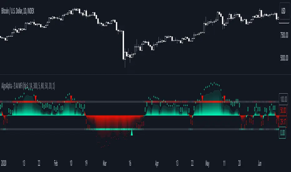
AI Adaptive Money Flow Index (Clustering) [AlgoAlpha]🌟🚀 Dive into the future of trading with our latest innovation: the AI Adaptive Money Flow Index by AlgoAlpha Indicator! 🚀🌟
Developed with the cutting-edge power of Machine Learning, this indicator is designed to revolutionize the way you view market dynamics. 🤖💹 With its unique blend of traditional Money Flow Index (MFI) analysis and advanced k-means clustering, it adapts to market conditions like never before.
Key Features:
📊 Adaptive MFI Analysis: Utilizes the classic MFI formula with a twist, adjusting its parameters based on AI-driven clustering.
🧠 AI-Driven Clustering: Applies k-means clustering to identify and adapt to market states, optimizing the MFI for current conditions.
🎨 Customizable Appearance: Offers adjustable settings for overbought, neutral, and oversold levels, as well as colors for uptrends and downtrends.
🔔 Alerts for Key Market Movements: Set alerts for trend reversals, overbought, and oversold conditions, ensuring you never miss a trading opportunity.
Quick Guide to Using the AI Adaptive MFI (Clustering):
🛠 Customize the Indicator: Customize settings like MFI source, length, and k-means clustering parameters to suit your analysis.
📈 Market Analysis: Monitor the dynamically adjusted overbought, neutral, and oversold levels for insights into market conditions. Watch for classification symbols ("+", "0", "-") for immediate understanding of the current market state. Look out for reversal signals (▲, ▼) to get potential entry points.
🔔 Set Alerts: Utilize the built-in alert conditions for trend changes, overbought, and oversold signals to stay ahead, even when you're not actively monitoring the charts.
How It Works:
The AI Adaptive Money Flow Index employs the k-means clustering machine learning algorithm to refine the traditional Money Flow Index, dynamically adjusting overbought, neutral, and oversold levels based on market conditions. This method analyzes historical MFI values, grouping them into initial clusters using the traditional MFI's overbought, oversold and neutral levels, and then finding the mean of each cluster, which represent the new market states thresholds. This adaptive approach ensures the indicator's sensitivity in real-time, offering a nuanced understanding of market trend and volume analysis.
By recalibrating MFI thresholds for each new data bar, the AI Adaptive MFI intelligently conforms to changing market dynamics. This process, assessing past periods to adjust the indicator's parameters, provides traders with insights finely tuned to recent market behavior. Such innovation enhances decision-making, leveraging the latest data to inform trading strategies. 🌐💥
Machine Learning: Multiple Logistic Regression
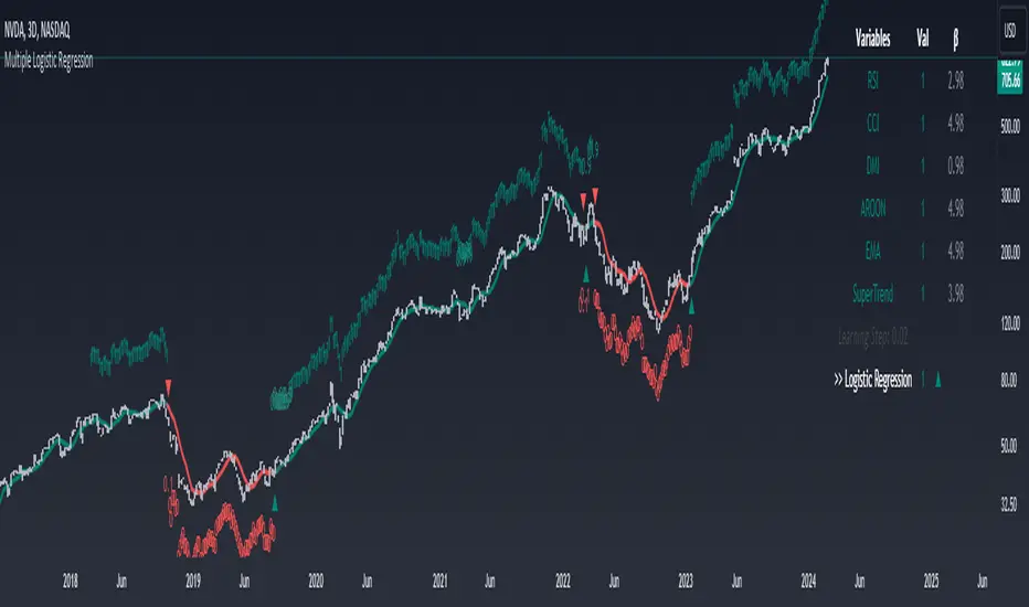
Multiple Logistic Regression Indicator
The Logistic Regression Indicator for TradingView is a versatile tool that employs multiple logistic regression based on various technical indicators to generate potential buy and sell signals. By utilizing key indicators such as RSI, CCI, DMI, Aroon, EMA, and SuperTrend, the indicator aims to provide a systematic approach to decision-making in financial markets.
How It Works:
Technical Indicators:
The script uses multiple technical indicators such as RSI, CCI, DMI, Aroon, EMA, and SuperTrend as input variables for the logistic regression model.
These indicators are normalized to create categorical variables, providing a consistent scale for the model.
Logistic Regression:
The logistic regression function is applied to the normalized input variables (x1 to x6) with user-defined coefficients (b0 to b6).
The logistic regression model predicts the probability of a binary outcome, with values closer to 1 indicating a bullish signal and values closer to 0 indicating a bearish signal.
Loss Function (Cross-Entropy Loss):
The cross-entropy loss function is calculated to quantify the difference between the predicted probability and the actual outcome.
The goal is to minimize this loss, which essentially measures the model's accuracy.
// Error Function (cross-entropy loss)
loss(y, p) =>
-y * math.log(p) - (1 - y) * math.log(1 - p)
// y - depended variable
// p - multiple logistic regression
Gradient Descent:
Gradient descent is an optimization algorithm used to minimize the loss function by adjusting the weights of the logistic regression model.
The script iteratively updates the weights (b1 to b6) based on the negative gradient of the loss function with respect to each weight.
// Adjusting model weights using gradient descent
b1 -= lr * (p + loss) * x1
b2 -= lr * (p + loss) * x2
b3 -= lr * (p + loss) * x3
b4 -= lr * (p + loss) * x4
b5 -= lr * (p + loss) * x5
b6 -= lr * (p + loss) * x6
// lr - learning rate or step of learning
// p - multiple logistic regression
// x_n - variables
Learning Rate:
The learning rate (lr) determines the step size in the weight adjustment process. It prevents the algorithm from overshooting the minimum of the loss function.
Users can set the learning rate to control the speed and stability of the optimization process.
Visualization:
The script visualizes the output of the logistic regression model by coloring the SMA.
Arrows are plotted at crossover and crossunder points, indicating potential buy and sell signals.
Lables are showing logistic regression values from 1 to 0 above and below bars
Table Display:
A table is displayed on the chart, providing real-time information about the input variables, their values, and the learned coefficients.
This allows traders to monitor the model's interpretation of the technical indicators and observe how the coefficients change over time.
How to Use:
Parameter Adjustment:
Users can adjust the length of technical indicators (rsi_length, cci_length, etc.) and the Z score length based on their preference and market characteristics.
Set the initial values for the regression coefficients (b0 to b6) and the learning rate (lr) according to your trading strategy.
Signal Interpretation:
Buy signals are indicated by an upward arrow (▲), and sell signals are indicated by a downward arrow (▼).
The color-coded SMA provides a visual representation of the logistic regression output by color.
Table Information:
Monitor the table for real-time information on the input variables, their values, and the learned coefficients.
Keep an eye on the learning rate to ensure a balance between model adjustment speed and stability.
Backtesting and Validation:
Before using the script in live trading, conduct thorough backtesting to evaluate its performance under different market conditions.
Validate the model against historical data to ensure its reliability.
Machine Learning Cross-Validation Split & Batch HighlighterThis indicator is designed for traders and analysts who employ Machine Learning (ML) techniques for cross-validation in financial markets.
The script visually segments a selected range of historical price data into splits and batches, helping in the assessment of model performance over different market conditions.
User
Theory
In ML, cross-validation is a technique to assess the generalizability of a model, typically by partitioning the data into a set of "folds" or "splits." Each split acts as a validation set, while the others form the training set. This script takes a unique approach by considering the sequential nature of financial time series data, where random shuffling of data (as in traditional cross-validation) can disrupt the temporal order, leading to misleading results.
Chronological Integrity of Splits
Even if the order of the splits is shuffled for cross-validation purposes, the data within each split remains in its original chronological sequence. This feature is crucial for time series analysis, as it respects the inherent order-dependency of financial markets. Thus, each split can be considered a microcosm of market behavior, maintaining the integrity of trends, cycles, and patterns that could be disrupted by random sampling.
The script allows users to define the number of splits and the size of each batch within a split. By doing so, it maintains the chronological sequence of the data, ensuring that the validation set is representative of a future time period that the model would predict.
www.tradingview.com
Parameters
Number of Splits: Defines how many segments the selected data range will be divided into. Each split serves as a standalone testing ground for the ML model. (Up to 24)
Batch Size: Determines the number of bars (candles) in each batch within a split. Smaller batches can help pinpoint overfitting at a finer granularity.
Start Index: The bar index from where the historical data range begins. It sets the starting point for data analysis.
End Index: The bar index where the historical data range ends. It marks the cutoff for data to be included in the model assessment.
Usage
To use this script effectively:
1 - Input the Start Index and End Index to define the historical data range you wish to analyze.
2 - Adjust the Number of Splits to create multiple validation sets for cross-validation.
3 - Set the Batch Size to control the granularity of each validation set within the splits.
4 - The script will highlight the background of each batch within the splits using alternating shades, allowing for a clear visual distinction of the data segmentation.
By maintaining the temporal sequence and allowing for adjustable granularity, the "ML Split and Batch Highlighter" aids in creating a robust validation framework for time series forecasting models in finance.

ML - Momentum Index (Pivots)Building upon the innovative foundations laid by Zeiierman's Machine Learning Momentum Index (MLMI), this variation introduces a series of refinements and new features aimed at bolstering the model's predictive accuracy and responsiveness. Licensed under the Creative Commons Attribution-NonCommercial-ShareAlike 4.0 International License (CC BY-NC-SA 4.0), my adaptation seeks to enhance the original by offering a more nuanced approach to momentum-based trading.
Key Features :
Pivot-Based Analysis: Shifting focus from trend crosses to pivot points, this version employs pivot bars to offer a distinct perspective on market momentum, aiding in the identification of critical reversal points.
Extended Parameter Set: By integrating additional parameters for making predictions, the model gains improved adaptability, allowing for finer tuning to match market conditions.
Dataset Size Limitation: To ensure efficiency and mitigate the risk of calculation timeouts, a cap on the dataset size has been implemented, balancing between comprehensive historical analysis and computational agility.
Enhanced Price Source Flexibility: Users can select between closing prices or (suggested) OHLC4 as the basis for calculations, tailoring the indicator to different analysis preferences and strategies.
This adaptation not only inherits the robust framework of the original MLMI but also introduces innovations to enhance its utility in diverse trading scenarios. Whether you're looking to refine your short-term trading tactics or seeking stable indicators for long-term strategies, the ML - Momentum Index (Pivots) offers a versatile tool to navigate the complexities of the market.
For a deeper understanding of the modifications and to leverage the full potential of this indicator, users are encouraged to explore the tooltips and documentation provided within the script.
The Momentum Indicator calculations have been transitioned to the MLMomentumIndex library, simplifying the process of integration. Users can now seamlessly incorporate the momentumIndexPivots function into their scripts to conduct detailed momentum analysis with ease.

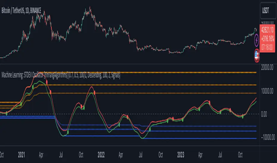
Machine Learning: STDEV Oscillator [YinYangAlgorithms]This Indicator aims to fill a gap within traditional Standard Deviation Analysis. Rather than its usual applications, this Indicator focuses on applying Standard Deviation within an Oscillator and likewise applying a Machine Learning approach to it. By doing so, we may hope to achieve an Adaptive Oscillator which can help display when the price is deviating from its standard movement. This Indicator may help display both when the price is Overbought or Underbought, and likewise, where the price may face Support and Resistance. The reason for this is that rather than simply plotting a Machine Learning Standard Deviation (STDEV), we instead create a High and a Low variant of STDEV, and then use its Highest and Lowest values calculated within another Deviation to create Deviation Zones. These zones may help to display these Support and Resistance locations; and likewise may help to show if the price is Overbought or Oversold based on its placement within these zones. This Oscillator may also help display Momentum when the High and/or Low STDEV crosses the midline (0). Lastly, this Oscillator may also be useful for seeing the spacing between the High and Low of the STDEV; large spacing may represent volatility within the STDEV which may be helpful for seeing when there is Momentum in the form of volatility.
Tutorial:
Above is an example of how this Indicator looks on BTC/USDT 1 Day. As you may see, when the price has parabolic movement, so does the STDEV. This is due to this price movement deviating from the mean of the data. Therefore when these parabolic movements occur, we create the Deviation Zones accordingly, in hopes that it may help to project future Support and Resistance locations as well as helping to display when the price is Overbought and Oversold.
If we zoom in a little bit, you may notice that the Support Zone (Blue) is smaller than the Resistance Zone (Orange). This is simply because during the last Bull Market there was more parabolic price deviation than there was during the Bear Market. You may see this if you refer to their values; the Resistance Zone goes to ~18k whereas the Support Zone is ~10.5k. This is completely normal and the way it is supposed to work. Due to the nature of how STDEV works, this Oscillator doesn’t use a 1:1 ratio and instead can develop and expand as exponential price action occurs.
The Neutral (0) line may also act as a Support and Resistance location. In the example above we can see how when the STDEV is below it, it acts as Resistance; and when it’s above it, it acts as Support.
This Neutral line may also provide us with insight as towards the momentum within the market and when it has shifted. When the STDEV is below the Neutral line, the market may be considered Bearish. When the STDEV is above the Neutral line, the market may be considered Bullish.
The Red Line represents the STDEV’s High and the Green Line represents the STDEV’s Low. When the STDEV’s High and Low get tight and close together, this may represent there is currently Low Volatility in the market. Low Volatility may cause consolidation to occur, however it also leaves room for expansion.
However, when the STDEV’s High and Low are quite spaced apart, this may represent High levels of Volatility in the market. This may mean the market is more prone to parabolic movements and expansion.
We will conclude our Tutorial here. Hopefully this has given you some insight into how applying Machine Learning to a High and Low STDEV then creating Deviation Zones based on it may help project when the Momentum of the Market is Bullish or Bearish; likewise when the price is Overbought or Oversold; and lastly where the price may face Support and Resistance in the form of STDEV.
If you have any questions, comments, ideas or concerns please don't hesitate to contact us.
HAPPY TRADING!
Optimal Length BackTester [YinYangAlgorithms]This Indicator allows for a ‘Optimal Length’ to be inputted within the Settings as a Source. Unlike most Indicators and/or Strategies that rely on either Static Lengths or Internal calculations for the length, this Indicator relies on the Length being derived from an external Indicator in the form of a Source Input.
This may not sound like much, but this application may allows limitless implementations of such an idea. By allowing the input of a Length within a Source Setting you may have an ‘Optimal Length’ that adjusts automatically without the need for manual intervention. This may allow for Traditional and Non-Traditional Indicators and/or Strategies to allow modifications within their settings as well to accommodate the idea of this ‘Optimal Length’ model to create an Indicator and/or Strategy that adjusts its length based on the top performing Length within the current Market Conditions.
This specific Indicator aims to allow backtesting with an ‘Optimal Length’ inputted as a ‘Source’ within the Settings.
This ‘Optimal Length’ may be used to display and potentially optimize multiple different Traditional Indicators within this BackTester. The following Traditional Indicators are included and available to be backtested with an ‘Optimal Length’ inputted as a Source in the Settings:
Moving Average; expressed as either a: Simple Moving Average, Exponential Moving Average or Volume Weighted Moving Average
Bollinger Bands; expressed based on the Moving Average Type
Donchian Channels; expressed based on the Moving Average Type
Envelopes; expressed based on the Moving Average Type
Envelopes Adjusted; expressed based on the Moving Average Type
All of these Traditional Indicators likewise may be displayed with multiple ‘Optimal Lengths’. They have the ability for multiple different ‘Optimal Lengths’ to be inputted and displayed, such as:
Fast Optimal Length
Slow Optimal Length
Neutral Optimal Length
By allowing for the input of multiple different ‘Optimal Lengths’ we may express the ‘Optimal Movement’ of such an expressed Indicator based on different Time Frames and potentially also movement based on Fast, Slow and Neutral (Inclusive) Lengths.
This in general is a simple Indicator that simply allows for the input of multiple different varieties of ‘Optimal Lengths’ to be displayed in different ways using Tradition Indicators. However, the idea and model of accepting a Length as a Source is unique and may be adopted in many different forms and endless ideas.
Tutorial:
You may add an ‘Optimal Length’ within the Settings as a ‘Source’ as followed in the example above. This Indicator allows for the input of a:
Neutral ‘Optimal Length’
Fast ‘Optimal Length’
Slow ‘Optimal Length’
It is important to account for all three as they generally encompass different min/max length values and therefore result in varying ‘Optimal Length’s’.
For instance, say you’re calculating the ‘Optimal Length’ and you use:
Min: 1
Max: 400
This would therefore be scanning for 400 (inclusive) lengths.
As a general way of calculating you may assume the following for which lengths are being used within an ‘Optimal Length’ calculation:
Fast: 1 - 199
Slow: 200 - 400
Neutral: 1 - 400
This allows for the calculation of a Fast and Slow length within the predetermined lengths allotted. However, it likewise allows for a Neutral length which is inclusive to all lengths alloted and may be deemed the ‘Most Accurate’ for these reasons. However, just because the Neutral is inclusive to all lengths, doesn’t mean the Fast and Slow lengths are irrelevant. The Fast and Slow length inputs may be useful for seeing how specifically zoned lengths may fair, and likewise when they cross over and/or under the Neutral ‘Optimal Length’.
This Indicator features the ability to display multiple different types of Traditional Indicators within the ‘Display Type’.
We will go over all of the different ‘Display Types’ with examples on how using a Fast, Slow and Neutral length would impact it:
Simple Moving Average:
In this example above have the Fast, Slow and Neutral Optimal Length formatted as a Slow Moving Average. The first example is on the 15 minute Time Frame and the second is on the 1 Day Time Frame, demonstrating how the length changes based on the Time Frame and the effects it may have.
Here we can see that by inputting ‘Optimal Lengths’ as a Simple Moving Average we may see moving averages that change over time with their ‘Optimal Lengths’. These lengths may help identify Support and/or Resistance locations. By using an 'Optimal Length' rather than a static length, we may create a Moving Average which may be more accurate as it attempts to be adaptive to current Market Conditions.
Bollinger Bands:
Bollinger Bands are a way to see a Simple Moving Average (SMA) that then uses Standard Deviation to identify how much deviation has occurred. This Deviation is then Added and Subtracted from the SMA to create the Bollinger Bands which help Identify possible movement zones that are ‘within range’. This may mean that the price may face Support / Resistance when it reaches the Outer / Inner bounds of the Bollinger Bands. Likewise, it may mean the Price is ‘Overbought’ when outside and above or ‘Underbought’ when outside and below the Bollinger Bands.
By applying All 3 different types of Optimal Lengths towards a Traditional Bollinger Band calculation we may hope to see different ranges of Bollinger Bands and how different lookback lengths may imply possible movement ranges on both a Short Term, Long Term and Neutral perspective. By seeing these possible ranges you may have the ability to identify more levels of Support and Resistance over different lengths and Trading Styles.
Donchian Channels:
Above you’ll see two examples of Machine Learning: Optimal Length applied to Donchian Channels. These are displayed with both the 15 Minute Time Frame and the 1 Day Time Frame.
Donchian Channels are a way of seeing potential Support and Resistance within a given lookback length. They are a way of withholding the High’s and Low’s of a specific lookback length and looking for deviation within this length. By applying a Fast, Slow and Neutral Machine Learning: Optimal Length to these Donchian Channels way may hope to achieve a viable range of High’s and Low’s that one may use to Identify Support and Resistance locations for different ranges of Optimal Lengths and likewise potentially different Trading Strategies.
Envelopes / Envelopes Adjusted:
Envelopes are an interesting one in the sense that they both may be perceived as useful; however we deem that with the use of an ‘Optimal Length’ that the ‘Envelopes Adjusted’ may work best. We will start with examples of the Traditional Envelope then showcase the Adjusted version.
Envelopes:
As you may see, a Traditional form of Envelopes even produced with a Machine Learning: Optimal Length may not produce optimal results. Unfortunately this may occur with some Traditional Indicators and they may need some adjustments as you’ll notice with the ‘Envelopes Adjusted’ version. However, even without the adjustments, these Envelopes may be useful for seeing ‘Overbought’ and ‘Oversold’ locations within a Machine Learning: Optimal Length standpoint.
Envelopes Adjusted:
By adding an adjustment to these Envelopes, we may hope to better reflect our Optimal Length within it. This is caused by adding a ratio reflection towards the current length of the Optimal Length and the max Length used. This allows for the Fast and Neutral (and potentially Slow if Neutral is greater) to achieve a potentially more accurate result.
Envelopes, much like Bollinger Bands are a way of seeing potential movement zones along with potential Support and Resistance. However, unlike Bollinger Bands which are based on Standard Deviation, Envelopes are based on percentages +/- from the Simple Moving Average.
We will conclude our Tutorial here. Hopefully this has given you some insight into how useful adding a ‘Optimal Length’ within an external (secondary) Indicator as a Source within the Settings may be. Likewise, how useful it may be for automation sake in the sense that when the ‘Optimal Length’ changes, it doesn’t rely on an alert where you need to manually update it yourself; instead it will update Automatically and you may reap the benefits of such with little manual input needed (aside from the initial setup).
If you have any questions, comments, ideas or concerns please don't hesitate to contact us.
HAPPY TRADING!

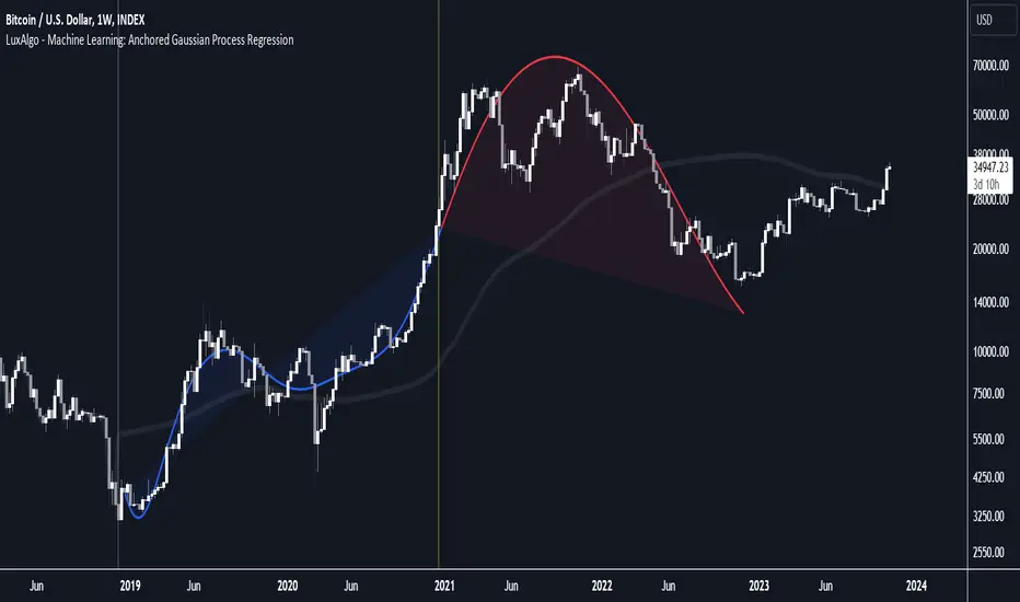
Machine Learning: Anchored Gaussian Process Regression [LuxAlgo]Machine Learning: Anchored Gaussian Process Regression is an anchored version of Machine Learning: Gaussian Process Regression .
It implements Gaussian Process Regression (GPR), a popular machine-learning method capable of estimating underlying trends in prices as well as forecasting them. Users can set a Training Window by choosing 2 points. GPR will be calculated for the data between these 2 points.
Do remember that forecasting trends in the market is challenging, do not use this tool as a standalone for your trading decisions.
🔶 USAGE
When adding the indicator to the chart, users will be prompted to select a starting and ending point for the calculations, click on your chart to select those points.
Start & end point are named 'Anchor 1' & 'Anchor 2', the Training Window is located between these 2 points. Once both points are positioned, the Training Window is set, whereafter the Gaussian Process Regression (GPR) is calculated using data between both Anchors .
The blue line is the GPR fit, the red line is the GPR prediction, derived from data between the Training Window .
Two user settings controlling the trend estimate are available, Smooth and Sigma.
Smooth determines the smoothness of our estimate, with higher values returning smoother results suitable for longer-term trend estimates.
Sigma controls the amplitude of the forecast, with values closer to 0 returning results with a higher amplitude.
One of the advantages of the anchoring process is the ability for the user to evaluate the accuracy of forecasts and further understand how settings affect their accuracy.
The publication also shows the mean average (faint silver line), which indicates the average of the prices within the calculation window (between the anchors). This can be used as a reference point for the forecast, seeing how it deviates from the training window average.
🔶 DETAILS
🔹 Limited Training Window
The Training Window is limited due to matrix.new() limitations in size.
When the 2 points are too far from each other (as in the latter example), the line will end at the maximum limit, without giving a size error.
The red forecasted line is always given priority.
🔹 Positioning Anchors
Typically Anchor 1 is located further in history than Anchor 2 , however, placing Anchor 2 before Anchor 1 is perfectly possibly, and won't give issues.
🔶 SETTINGS
Anchor 1 / Anchor 2: both points will form the Training Window .
Forecasting Length: Forecasting horizon, determines how many bars in the 'future' are forecasted.
Smooth: Controls the degree of smoothness of the model fit.
Sigma: Noise variance. Controls the amplitude of the forecast, lower values will make it more sensitive to outliers.
Machine Learning: VWAP [YinYangAlgorithms]Machine Learning: VWAP aims to use Machine Learning to Identify the best location to Anchor the VWAP at. Rather than using a traditional fixed length or simply adjusting based on a Date / Time; by applying Machine Learning we may hope to identify crucial areas which make sense to reset the VWAP and start anew. VWAP’s may act similar to a Bollinger Band in the sense that they help to identify both Overbought and Oversold Price locations based on previous movements and help to identify how far the price may move within the current Trend. However, unlike Bollinger Bands, VWAPs have the ability to parabolically get quite spaced out and also reset. For this reason, the price may never actually go from the Lower to the Upper and vice versa (when very spaced out; when the Upper and Lower zones are narrow, it may bounce between the two). The reason for this is due to how the anchor location is calculated and in this specific Indicator, how it changes anchors based on price movement calculated within Machine Learning.
This Indicator changes the anchor if the Low < Lowest Low of a length of X and likewise if the High > Highest High of a length of X. This logic is applied within a Machine Learning standpoint that likewise amplifies this Lookback Length by adding a Machine Learning Length to it and increasing the lookback length even further.
Due to how the anchor for this VWAP changes, you may notice that the Basis Line (Orange) may act as a Trend Identifier. When the Price is above the basis line, it may represent a bullish trend; and likewise it may represent a bearish trend when below it. You may also notice what may happen is when the trend occurs, it may push all the way to the Upper or Lower levels of this VWAP. It may then proceed to move horizontally until the VWAP expands more and it may gain more movement; or it may correct back to the Basis Line. If it corrects back to the basis line, what may happen is it either uses the Basis Line as a Support and continues in its current direction, or it will change the VWAP anchor and start anew.
Tutorial:
If we zoom in on the most recent VWAP we can see how it expands. Expansion may be caused by time but generally it may be caused by price movement and volume. Exponential Price movement causes the VWAP to expand, even if there are corrections to it. However, please note Volume adds a large weighted factor to the calculation; hence Volume Weighted Average Price (VWAP).
If you refer to the white circle in the example above; you’ll be able to see that the VWAP expanded even while the price was correcting to the Basis line. This happens due to exponential movement which holds high volume. If you look at the volume below the white circle, you’ll notice it was very large; however even though there was exponential price movement after the white circle, since the volume was low, the VWAP didn’t expand much more than it already had.
There may be times where both Volume and Price movement isn’t significant enough to cause much of an expansion. During this time it may be considered to be in a state of consolidation. While looking at this example, you may also notice the color switch from red to green to red. The color of the VWAP is related to the movement of the Basis line (Orange middle line). When the current basis is > the basis of the previous bar the color of the VWAP is green, and when the current basis is < the basis of the previous bar, the color of the VWAP is red. The color may help you gauge the current directional movement the price is facing within the VWAP.
You may have noticed there are signals within this Indicator. These signals are composed of Green and Red Triangles which represent potential Bullish and Bearish momentum changes. The Momentum changes happen when the Signal Type:
The High/Low or Close (You pick in settings)
Crosses one of the locations within the VWAP.
Bullish Momentum change signals occur when :
Signal Type crosses OVER the Basis
Signal Type crosses OVER the lower level
Bearish Momentum change signals occur when:
Signal Type crosses UNDER the Basis
Signal Type Crosses UNDER the upper level
These signals may represent locations where momentum may occur in the direction of these signals. For these reasons there are also alerts available to be set up for them.
If you refer to the two circles within the example above, you may see that when the close goes above the basis line, how it mat represents bullish momentum. Likewise if it corrects back to the basis and the basis acts as a support, it may continue its bullish momentum back to the upper levels again. However, if you refer to the red circle, you’ll see if the basis fails to act as a support, it may then start to correct all the way to the lower levels, or depending on how expanded the VWAP is, it may just reset its anchor due to such drastic movement.
You also have the ability to disable Machine Learning by setting ‘Machine Learning Type’ to ‘None’. If this is done, it will go off whether you have it set to:
Bullish
Bearish
Neutral
For the type of VWAP you want to see. In this example above we have it set to ‘Bullish’. Non Machine Learning VWAP are still calculated using the same logic of if low < lowest low over length of X and if high > highest high over length of X.
Non Machine Learning VWAP’s change much quicker but may also allow the price to correct from one side to the other without changing VWAP Anchor. They may be useful for breaking up a trend into smaller pieces after momentum may have changed.
Above is an example of how the Non Machine Learning VWAP looks like when in Bearish. As you can see based on if it is Bullish or Bearish is how it favors the trend to be and may likewise dictate when it changes the Anchor.
When set to neutral however, the Anchor may change quite quickly. This results in a still useful VWAP to help dictate possible zones that the price may move within, but they’re also much tighter zones that may not expand the same way.
We will conclude this Tutorial here, hopefully this gives you some insight as to why and how Machine Learning VWAPs may be useful; as well as how to use them.
Settings:
VWAP:
VWAP Type: Type of VWAP. You can favor specific direction changes or let it be Neutral where there is even weight to both. Please note, these do not apply to the Machine Learning VWAP.
Source: VWAP Source. By default VWAP usually uses HLC3; however OHLC4 may help by providing more data.
Lookback Length: The Length of this VWAP when it comes to seeing if the current High > Highest of this length; or if the current Low is < Lowest of this length.
Standard VWAP Multiplier: This multiplier is applied only to the Standard VWMA. This is when 'Machine Learning Type' is set to 'None'.
Machine Learning:
Use Rational Quadratics: Rationalizing our source may be beneficial for usage within ML calculations.
Signal Type: Bullish and Bearish Signals are when the price crosses over/under the basis, as well as the Upper and Lower levels. These may act as indicators to where price movement may occur.
Machine Learning Type: Are we using a Simple ML Average, KNN Mean Average, KNN Exponential Average or None?
KNN Distance Type: We need to check if distance is within the KNN Min/Max distance, which distance checks are we using.
Machine Learning Length: How far back is our Machine Learning going to keep data for.
k-Nearest Neighbour (KNN) Length: How many k-Nearest Neighbours will we account for?
Fast ML Data Length: What is our Fast ML Length? This is used with our Slow Length to create our KNN Distance.
Slow ML Data Length: What is our Slow ML Length? This is used with our Fast Length to create our KNN Distance.
If you have any questions, comments, ideas or concerns please don't hesitate to contact us.
HAPPY TRADING!

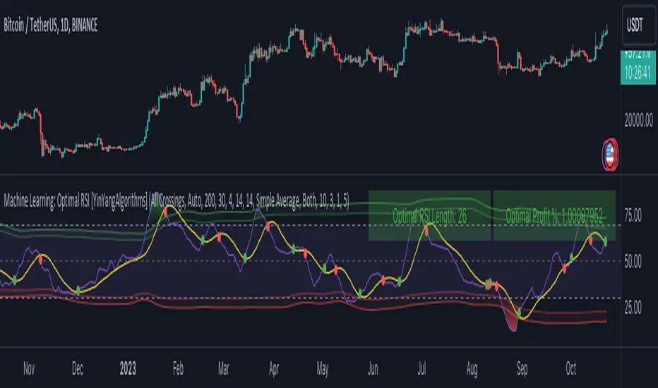
Machine Learning: Optimal RSI [YinYangAlgorithms]This Indicator, will rate multiple different lengths of RSIs to determine which RSI to RSI MA cross produced the highest profit within the lookback span. This ‘Optimal RSI’ is then passed back, and if toggled will then be thrown into a Machine Learning calculation. You have the option to Filter RSI and RSI MA’s within the Machine Learning calculation. What this does is, only other Optimal RSI’s which are in the same bullish or bearish direction (is the RSI above or below the RSI MA) will be added to the calculation.
You can either (by default) use a Simple Average; which is essentially just a Mean of all the Optimal RSI’s with a length of Machine Learning. Or, you can opt to use a k-Nearest Neighbour (KNN) calculation which takes a Fast and Slow Speed. We essentially turn the Optimal RSI into a MA with different lengths and then compare the distance between the two within our KNN Function.
RSI may very well be one of the most used Indicators for identifying crucial Overbought and Oversold locations. Not only that but when it crosses its Moving Average (MA) line it may also indicate good locations to Buy and Sell. Many traders simply use the RSI with the standard length (14), however, does that mean this is the best length?
By using the length of the top performing RSI and then applying some Machine Learning logic to it, we hope to create what may be a more accurate, smooth, optimal, RSI.
Tutorial:
This is a pretty zoomed out Perspective of what the Indicator looks like with its default settings (except with Bollinger Bands and Signals disabled). If you look at the Tables above, you’ll notice, currently the Top Performing RSI Length is 13 with an Optimal Profit % of: 1.00054973. On its default settings, what it does is Scan X amount of RSI Lengths and checks for when the RSI and RSI MA cross each other. It then records the profitability of each cross to identify which length produced the overall highest crossing profitability. Whichever length produces the highest profit is then the RSI length that is used in the plots, until another length takes its place. This may result in what we deem to be the ‘Optimal RSI’ as it is an adaptive RSI which changes based on performance.
In our next example, we changed the ‘Optimal RSI Type’ from ‘All Crossings’ to ‘Extremity Crossings’. If you compare the last two examples to each other, you’ll notice some similarities, but overall they’re quite different. The reason why is, the Optimal RSI is calculated differently. When using ‘All Crossings’ everytime the RSI and RSI MA cross, we evaluate it for profit (short and long). However, with ‘Extremity Crossings’, we only evaluate it when the RSI crosses over the RSI MA and RSI <= 40 or RSI crosses under the RSI MA and RSI >= 60. We conclude the crossing when it crosses back on its opposite of the extremity, and that is how it finds its Optimal RSI.
The way we determine the Optimal RSI is crucial to calculating which length is currently optimal.
In this next example we have zoomed in a bit, and have the full default settings on. Now we have signals (which you can set alerts for), for when the RSI and RSI MA cross (green is bullish and red is bearish). We also have our Optimal RSI Bollinger Bands enabled here too. These bands allow you to see where there may be Support and Resistance within the RSI at levels that aren’t static; such as 30 and 70. The length the RSI Bollinger Bands use is the Optimal RSI Length, allowing it to likewise change in correlation to the Optimal RSI.
In the example above, we’ve zoomed out as far as the Optimal RSI Bollinger Bands go. You’ll notice, the Bollinger Bands may act as Support and Resistance locations within and outside of the RSI Mid zone (30-70). In the next example we will highlight these areas so they may be easier to see.
Circled above, you may see how many times the Optimal RSI faced Support and Resistance locations on the Bollinger Bands. These Bollinger Bands may give a second location for Support and Resistance. The key Support and Resistance may still be the 30/50/70, however the Bollinger Bands allows us to have a more adaptive, moving form of Support and Resistance. This helps to show where it may ‘bounce’ if it surpasses any of the static levels (30/50/70).
Due to the fact that this Indicator may take a long time to execute and it can throw errors for such, we have added a Setting called: Adjust Optimal RSI Lookback and RSI Count. This settings will automatically modify the Optimal RSI Lookback Length and the RSI Count based on the Time Frame you are on and the Bar Indexes that are within. For instance, if we switch to the 1 Hour Time Frame, it will adjust the length from 200->90 and RSI Count from 30->20. If this wasn’t adjusted, the Indicator would Timeout.
You may however, change the Setting ‘Adjust Optimal RSI Lookback and RSI Count’ to ‘Manual’ from ‘Auto’. This will give you control over the ‘Optimal RSI Lookback Length’ and ‘RSI Count’ within the Settings. Please note, it will likely take some “fine tuning” to find working settings without the Indicator timing out, but there are definitely times you can find better settings than our ‘Auto’ will create; especially on higher Time Frames. The Minimum our ‘Auto’ will create is:
Optimal RSI Lookback Length: 90
RSI Count: 20
The Maximum it will create is:
Optimal RSI Lookback Length: 200
RSI Count: 30
If there isn’t much bar index history, for instance, if you’re on the 1 Day and the pair is BTC/USDT you’ll get < 4000 Bar Indexes worth of data. For this reason it is possible to manually increase the settings to say:
Optimal RSI Lookback Length: 500
RSI Count: 50
But, please note, if you make it too high, it may also lead to inaccuracies.
We will conclude our Tutorial here, hopefully this has given you some insight as to how calculating our Optimal RSI and then using it within Machine Learning may create a more adaptive RSI.
Settings:
Optimal RSI:
Show Crossing Signals: Display signals where the RSI and RSI Cross.
Show Tables: Display Information Tables to show information like, Optimal RSI Length, Best Profit, New Optimal RSI Lookback Length and New RSI Count.
Show Bollinger Bands: Show RSI Bollinger Bands. These bands work like the TDI Indicator, except its length changes as it uses the current RSI Optimal Length.
Optimal RSI Type: This is how we calculate our Optimal RSI. Do we use all RSI and RSI MA Crossings or just when it crosses within the Extremities.
Adjust Optimal RSI Lookback and RSI Count: Auto means the script will automatically adjust the Optimal RSI Lookback Length and RSI Count based on the current Time Frame and Bar Index's on chart. This will attempt to stop the script from 'Taking too long to Execute'. Manual means you have full control of the Optimal RSI Lookback Length and RSI Count.
Optimal RSI Lookback Length: How far back are we looking to see which RSI length is optimal? Please note the more bars the lower this needs to be. For instance with BTC/USDT you can use 500 here on 1D but only 200 for 15 Minutes; otherwise it will timeout.
RSI Count: How many lengths are we checking? For instance, if our 'RSI Minimum Length' is 4 and this is 30, the valid RSI lengths we check is 4-34.
RSI Minimum Length: What is the RSI length we start our scans at? We are capped with RSI Count otherwise it will cause the Indicator to timeout, so we don't want to waste any processing power on irrelevant lengths.
RSI MA Length: What length are we using to calculate the optimal RSI cross' and likewise plot our RSI MA with?
Extremity Crossings RSI Backup Length: When there is no Optimal RSI (if using Extremity Crossings), which RSI should we use instead?
Machine Learning:
Use Rational Quadratics: Rationalizing our Close may be beneficial for usage within ML calculations.
Filter RSI and RSI MA: Should we filter the RSI's before usage in ML calculations? Essentially should we only use RSI data that are of the same type as our Optimal RSI? For instance if our Optimal RSI is Bullish (RSI > RSI MA), should we only use ML RSI's that are likewise bullish?
Machine Learning Type: Are we using a Simple ML Average, KNN Mean Average, KNN Exponential Average or None?
KNN Distance Type: We need to check if distance is within the KNN Min/Max distance, which distance checks are we using.
Machine Learning Length: How far back is our Machine Learning going to keep data for.
k-Nearest Neighbour (KNN) Length: How many k-Nearest Neighbours will we account for?
Fast ML Data Length: What is our Fast ML Length? This is used with our Slow Length to create our KNN Distance.
Slow ML Data Length: What is our Slow ML Length? This is used with our Fast Length to create our KNN Distance.
If you have any questions, comments, ideas or concerns please don't hesitate to contact us.
HAPPY TRADING!
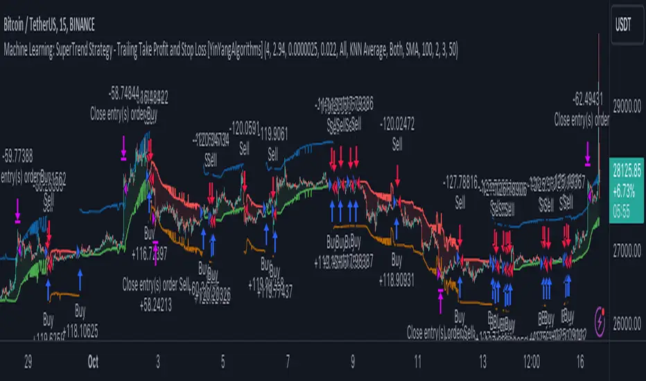
Machine Learning: SuperTrend Strategy TP/SL [YinYangAlgorithms]The SuperTrend is a very useful Indicator to display when trends have shifted based on the Average True Range (ATR). Its underlying ideology is to calculate the ATR using a fixed length and then multiply it by a factor to calculate the SuperTrend +/-. When the close crosses the SuperTrend it changes direction.
This Strategy features the Traditional SuperTrend Calculations with Machine Learning (ML) and Take Profit / Stop Loss applied to it. Using ML on the SuperTrend allows for the ability to sort data from previous SuperTrend calculations. We can filter the data so only previous SuperTrends that follow the same direction and are within the distance bounds of our k-Nearest Neighbour (KNN) will be added and then averaged. This average can either be achieved using a Mean or with an Exponential calculation which puts added weight on the initial source. Take Profits and Stop Losses are then added to the ML SuperTrend so it may capitalize on Momentum changes meanwhile remaining in the Trend during consolidation.
By applying Machine Learning logic and adding a Take Profit and Stop Loss to the Traditional SuperTrend, we may enhance its underlying calculations with potential to withhold the trend better. The main purpose of this Strategy is to minimize losses and false trend changes while maximizing gains. This may be achieved by quick reversals of trends where strategic small losses are taken before a large trend occurs with hopes of potentially occurring large gain. Due to this logic, the Win/Loss ratio of this Strategy may be quite poor as it may take many small marginal losses where there is consolidation. However, it may also take large gains and capitalize on strong momentum movements.
Tutorial:
In this example above, we can get an idea of what the default settings may achieve when there is momentum. It focuses on attempting to hit the Trailing Take Profit which moves in accord with the SuperTrend just with a multiplier added. When momentum occurs it helps push the SuperTrend within it, which on its own may act as a smaller Trailing Take Profit of its own accord.
We’ve highlighted some key points from the last example to better emphasize how it works. As you can see, the White Circle is where profit was taken from the ML SuperTrend simply from it attempting to switch to a Bullish (Buy) Trend. However, that was rejected almost immediately and we went back to our Bearish (Sell) Trend that ended up resulting in our Take Profit being hit (Yellow Circle). This Strategy aims to not only capitalize on the small profits from SuperTrend to SuperTrend but to also capitalize when the Momentum is so strong that the price moves X% away from the SuperTrend and is able to hit the Take Profit location. This Take Profit addition to this Strategy is crucial as momentum may change state shortly after such drastic price movements; and if we were to simply wait for it to come back to the SuperTrend, we may lose out on lots of potential profit.
If you refer to the Yellow Circle in this example, you’ll notice what was talked about in the Summary/Overview above. During periods of consolidation when there is little momentum and price movement and we don’t have any Stop Loss activated, you may see ‘Signal Flashing’. Signal Flashing is when there are Buy and Sell signals that keep switching back and forth. During this time you may be taking small losses. This is a normal part of this Strategy. When a signal has finally been confirmed by Momentum, is when this Strategy shines and may produce the profit you desire.
You may be wondering, what causes these jagged like patterns in the SuperTrend? It's due to the ML logic, and it may be a little confusing, but essentially what is happening is the Fast Moving SuperTrend and the Slow Moving SuperTrend are creating KNN Min and Max distances that are extreme due to (usually) parabolic movement. This causes fewer values to be added to and averaged within the ML and causes less smooth and more exponential drastic movements. This is completely normal, and one of the perks of using k-Nearest Neighbor for ML calculations. If you don’t know, the Min and Max Distance allowed is derived from the most recent(0 index of data array) to KNN Length. So only SuperTrend values that exhibit distances within these Min/Max will be allowed into the average.
Since the KNN ML logic can cause these exponential movements in the SuperTrend, they likewise affect its Take Profit. The Take Profit may benefit from this movement like displayed in the example above which helped it claim profit before then exhibiting upwards movement.
By default our Stop Loss Multiplier is kept quite low at 0.0000025. Keeping it low may help to reduce some Signal Flashing while not taking extra losses more so than not using it at all. However, if we increase it even more to say 0.005 like is shown in the example above. It can really help the trend keep momentum. Please note, although previous results don’t imply future results, at 0.0000025 Stop Loss we are currently exhibiting 69.27% profit while at 0.005 Stop Loss we are exhibiting 33.54% profit. This just goes to show that although there may be less Signal Flashing, it may not result in more profit.
We will conclude our Tutorial here. Hopefully this has given you some insight as to how Machine Learning, combined with Trailing Take Profit and Stop Loss may have positive effects on the SuperTrend when turned into a Strategy.
Settings:
SuperTrend:
ATR Length: ATR Length used to create the Original Supertrend.
Factor: Multiplier used to create the Original Supertrend.
Stop Loss Multiplier: 0 = Don't use Stop Loss. Stop loss can be useful for helping to prevent false signals but also may result in more loss when hit and less profit when switching trends.
Take Profit Multiplier: Take Profits can be useful within the Supertrend Strategy to stop the price reverting all the way to the Stop Loss once it's been profitable.
Machine Learning:
Only Factor Same Trend Direction: Very useful for ensuring that data used in KNN is not manipulated by different SuperTrend Directional data. Please note, it doesn't affect KNN Exponential.
Rationalized Source Type: Should we Rationalize only a specific source, All or None?
Machine Learning Type: Are we using a Simple ML Average, KNN Mean Average, KNN Exponential Average or None?
Machine Learning Smoothing Type: How should we smooth our Fast and Slow ML Datas to be used in our KNN Distance calculation? SMA, EMA or VWMA?
KNN Distance Type: We need to check if distance is within the KNN Min/Max distance, which distance checks are we using.
Machine Learning Length: How far back is our Machine Learning going to keep data for.
k-Nearest Neighbour (KNN) Length: How many k-Nearest Neighbours will we account for?
Fast ML Data Length: What is our Fast ML Length?? This is used with our Slow Length to create our KNN Distance.
Slow ML Data Length: What is our Slow ML Length?? This is used with our Fast Length to create our KNN Distance.
If you have any questions, comments, ideas or concerns please don't hesitate to contact us.
HAPPY TRADING!
Machine Learning using Neural Networks | EducationalThe script provided is a comprehensive illustration of how to implement and execute a simplistic Neural Network (NN) on TradingView using PineScript.
It encompasses the entire workflow from data input, weight initialization, implicit neuron calculation, feedforward computation, backpropagation for weight adjustments, generating predictions, to visualizing the Mean Squared Error (MSE) Loss Curve for monitoring the training phase.
In the visual example above, you can see that the prediction is not aligned with the actual value. This is intentional for demonstrative purposes, and by incrementing the Epochs or Learning Rate, you will see these two values converge as the accuracy increases.
Hyperparameters:
Learning Rate, Epochs, and the choice between Simple Backpropagation and a verbose version are declared as script inputs, allowing users to tailor the training process.
Initialization:
Random initialization of weight matrices (w1, w2) is performed to ensure asymmetry, promoting effective gradient updates. A seed is added for reproducibility.
Utility Functions:
Functions for matrix randomization, sigmoid activation, MSE loss calculation, data normalization, and standardization are defined to streamline the computation process.
Neural Network Computation:
The feedforward function computes the hidden and output layer values given the input.
Two variants of the backpropagation function are provided for weight adjustment, with one offering a more verbose step-by-step computation of gradients.
A wrapper train_nn function iterates through epochs, performing feedforward, loss computation, and backpropagation in each epoch while logging and collecting loss values.
Training Invocation:
The input data is prepared by normalizing it to a value between 0 and 1 using the maximum standardized value, and the training process is invoked only on the last confirmed bar to preserve computational resources.
Output Forecasting and Visualization:
Post training, the NN's output (predicted price) is computed, standardized and visualized alongside the actual price on the chart.
The MSE loss between the predicted and actual prices is visualized, providing insight into the prediction accuracy.
Optionally, the MSE Loss Curve is plotted on the chart, illustrating the loss trajectory through epochs, assisting in understanding the training performance.
Customizable Visualization:
Various inputs control visualization aspects like Chart Scaling, Chart Horizontal Offset, and Chart Vertical Offset, allowing users to adapt the visualization to their preference.
-------------------------------------------------------
The following is this Neural Network structure, consisting of one hidden layer, with two hidden neurons.
Through understanding the steps outlined in my code, one should be able to scale the NN in any way they like, such as changing the input / output data and layers to fit their strategy ideas.
Additionally, one could forgo the backpropagation function, and load their own trained weights into the w1 and w2 matrices, to have this code run purely for inference.
-------------------------------------------------------
While this demonstration does create a “prediction”, it is on historical data. The purpose here is educational, rather than providing a ready tool for non-programmer consumers.
Normally in Machine Learning projects, the training process would be split into two segments, the Training and the Validation parts. For the purpose of conveying the core concept in a concise and non-repetitive way, I have foregone the Validation part. However, it is merely the application of your trained network on new data (feedforward), and monitoring the loss curve.
Essentially, checking the accuracy on “unseen” data, while training it on “seen” data.
-------------------------------------------------------
I hope that this code will help developers create interesting machine learning applications within the Tradingview ecosystem.

Machine Learning: Gaussian Process Regression [LuxAlgo]We provide an implementation of the Gaussian Process Regression (GPR), a popular machine-learning method capable of estimating underlying trends in prices as well as forecasting them.
While this implementation is adapted to real-time usage, do remember that forecasting trends in the market is challenging, do not use this tool as a standalone for your trading decisions.
🔶 USAGE
The main goal of our implementation of GPR is to forecast trends. The method is applied to a subset of the most recent prices, with the Training Window determining the size of this subset.
Two user settings controlling the trend estimate are available, Smooth and Sigma . Smooth determines the smoothness of our estimate, with higher values returning smoother results suitable for longer-term trend estimates.
Sigma controls the amplitude of the forecast, with values closer to 0 returning results with a higher amplitude. Do note that due to the calculation of the method, lower values of sigma can return errors with higher values of the training window.
🔹 Updating Mechanisms
The script includes three methods to update a forecast. By default a forecast will not update for new bars (Lock Forecast).
The forecast can be re-estimated once the price reaches the end of the forecasting window when using the "Update Once Reached" method.
Finally "Continuously Update" will update the whole forecast on any new bar.
🔹 Estimating Trends
Gaussian Process Regression can be used to estimate past underlying local trends in the price, allowing for a noise-free interpretation of trends.
This can be useful for performing descriptive analysis, such as highlighting patterns more easily.
🔶 SETTINGS
Training Window: Number of most recent price observations used to fit the model
Forecasting Length: Forecasting horizon, determines how many bars in the future are forecasted.
Smooth: Controls the degree of smoothness of the model fit.
Sigma: Noise variance. Controls the amplitude of the forecast, lower values will make it more sensitive to outliers.
Update: Determines when the forecast is updated, by default the forecast is not updated for new bars.

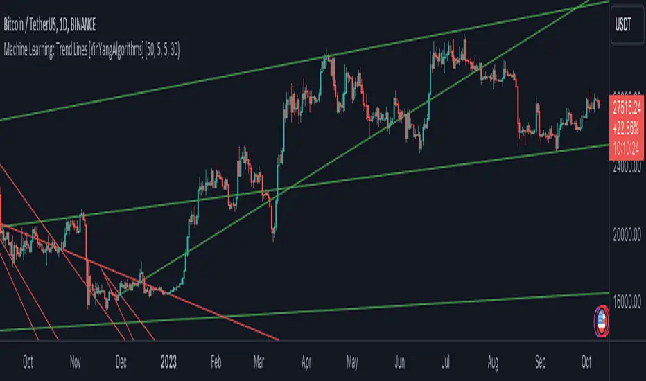
Machine Learning: Trend Lines [YinYangAlgorithms]Trend lines have always been a key indicator that may help predict many different types of price movements. They have been well known to create different types of formations such as: Pennants, Channels, Flags and Wedges. The type of formation they create is based on how the formation was created and the angle it was created. For instance, if there was a strong price increase and then there is a Wedge where both end points meet, this is considered a Bull Pennant. The formations Trend Lines create may be powerful tools that can help predict current Support and Resistance and also Future Momentum changes. However, not all Trend Lines will create formations, and alone they may stand as strong Support and Resistance locations on the Vertical.
The purpose of this Indicator is to apply Machine Learning logic to a Traditional Trend Line Calculation, and therefore allowing a new approach to a modern indicator of high usage. The results of such are quite interesting and goes to show the impacts a simple KNN Machine Learning model can have on Traditional Indicators.
Tutorial:
There are a few different settings within this Indicator. Many will greatly impact the results and if any are changed, lots will need ‘Fine Tuning’. So let's discuss the main toggles that have great effects and what they do before discussing the lengths. Currently in this example above we have the Indicator at its Default Settings. In this example, you can see how the Trend Lines act as key Support and Resistance locations. Due note, Support and Resistance are a relative term, as is their color. What starts off as Support or Resistance may change when the price crosses over / under them.
In the example above we have zoomed in and circled locations that exhibited markers of Support and Resistance along the Trend Lines. These Trend Lines are all created using the Default Settings. As you can see from the example above; just because it is a Green Upwards Trend Line, doesn’t mean it’s a Support Line. Support and Resistance is always shifting on Trend Lines based on the prices location relative to them.
We won’t go through all the Formations Trend Lines make, but the example above, we can see the Trend Lines formed a Downward Channel. Channels are when there are two parallel downwards Trend Lines that are at a relatively similar angle. This means that they won’t ever meet. What may happen when the price is within these channels, is it may bounce between the upper and lower bounds. These Channels may drive the price upwards or downwards, depending on if it is in an Upwards or Downwards Channel.
If you refer to the example above, you’ll notice that the Trend Lines are formed like traditional Trend Lines. They don’t stem from current Highs and Lows but rather Machine Learning Highs and Lows. More often than not, the Machine Learning approach to Trend Lines cause their start point and angle to be quite different than a Traditional Trend Line. Due to this, it may help predict Support and Resistance locations at are more uncommon and therefore can be quite useful.
In the example above we have turned off the toggle in Settings ‘Use Exponential Data Average’. This Settings uses a custom Exponential Data Average of the KNN rather than simply averaging the KNN. By Default it is enabled, but as you can see when it is disabled it may create some pretty strong lasting Trend Lines. This is why we advise you ZOOM OUT AS FAR AS YOU CAN. Trend Lines are only displayed when you’ve zoomed out far enough that their Start Point is visible.
As you can see in this example above, there were 3 major Upward Trend Lines created in 2020 that have had a major impact on Support and Resistance Locations within the last year. Lets zoom in and get a closer look.
We have zoomed in for this example above, and circled some of the major Support and Resistance locations that these Upward Trend Lines may have had a major impact on.
Please note, these Machine Learning Trend Lines aren’t a ‘One Size Fits All’ kind of thing. They are completely customizable within the Settings, so that you can get a tailored experience based on what Pair and Time Frame you are trading on.
When any values are changed within the Settings, you’ll likely need to ‘Fine Tune’ the rest of the settings until your desired result is met. By default the modifiable lengths within the Settings are:
Machine Learning Length: 50
KNN Length:5
Fast ML Data Length: 5
Slow ML Data Length: 30
For example, let's toggle ‘Use Exponential Data Averages’ back on and change ‘Fast ML Data Length’ from 5 to 20 and ‘Slow ML Data Length’ from 30 to 50.
As you can in the example above, all of the lines have changed. Although there are still some strong Support Locations created by the Upwards Trend Lines.
We will conclude our Tutorial here. Hopefully you’ve learned how to use Machine Learning Trend Lines and will be able to now see some more unorthodox Support and Resistance locations on the Vertical.
Settings:
Use Machine Learning Sources: If disabled Traditional Trend line sources (High and Low) will be used rather than Rational Quadratics.
Use KNN Distance Sorting: You can disable this if you wish to not have the Machine Learning Data sorted using KNN. If disabled trend line logic will be Traditional.
Use Exponential Data Average: This Settings uses a custom Exponential Data Average of the KNN rather than simply averaging the KNN.
Machine Learning Length: How strong is our Machine Learning Memory? Please note, when this value is too high the data is almost 'too' much and can lead to poor results.
K-Nearest Neighbour (KNN) Length: How many K-Nearest Neighbours are allowed with our Distance Clustering? Please note, too high or too low may lead to poor results.
Fast ML Data Length: Fast and Slow speed needs to be adjusted properly to see results. 3/5/7 all seem to work well for Fast.
Slow ML Data Length: Fast and Slow speed needs to be adjusted properly to see results. 20 - 50 all seem to work well for Slow.
If you have any questions, comments, ideas or concerns please don't hesitate to contact us.
HAPPY TRADING!
Machine Learning: MFI Heat Map [YinYangAlgorithms]Overview:
MFI Heat Maps are a visually appealing way to display the values of 29 different MFIs at the same time while being able to make sense of it. Each plot within the Indicator represents a different MFI value. The higher you get up, the longer the length that was used for this MFI. This Indicator also features the use of Machine Learning to help balance the MFI levels. It doesn’t solely rely upon Machine Learning but instead incorporates a growing length MFI averaged with the Machine Learning MFI at any given index.
For instance, say we are calculating the 10th plot from the bottom, the MFI would be an average of:
MFI(source, 11)
Machine Learning MFI at Index of 10
We do it this way as they both help smooth each other out without relying solely on just one calculation method.
Due to plot limitations, you are capped at 28 Plot Amounts within this indicator, but that is still quite a bit of information you can glean from a Heat Map.
The Machine Learning used in this indicator is of the K-Nearest Neighbor (KNN). It uses a Fast and Slow MFI calculation then sorts through them over Machine Learning Length and calculates the differences between them. It then slices off KNN length to create our Max/Min Distances allotted. It adds the average between Fast and Slow MFIs to a Viable Distances array if their distances are within the KNN Min/Max distance. It then averages all distances in the Viable Distances array and returns the result.
The result of the KNN Function is saved to another ML Data array whose length is that of Plot Amount (Heat Map Size). This way each Index of the ML Data array can be indexed according to the Heat Map Size.
The Average of the ML Data array is the MFI line (white) that you’ll see plotted on the Indicator. There is also the SMA of the MFI Average (orange) which is likewise plotted. These plots allow you to visualize where the ML MFI is sitting and can potentially be useful for seeing when the MFI Average and SMA cross over and under each other.
We’ve heard many people talk highly of RSI, but sadly not too many even refer to MFI. MFI oftentimes may be overlooked, especially with new traders who may not even know what it is. Essentially MFI is an RSI but it also incorporates Volume into its calculations, which in our opinion leads to a more accurate reading; afterall, what is price movement without Volume.
Tutorial:
You may be thinking, this Indicator looks appealing to the eye, but how do I benefit from it trading wise?
Before we get into our visual examples, let's talk briefly about what makes Heat Maps in general a useful tool for trading. Heat Maps give us the ability to visualize and understand lots of data while removing the clutter. We can understand the data of 29 different MFIs without having to look at and decipher 29 different MFI plots. When you overlay too many MFI lines on top of each other, they can be very difficult to read and oftentimes end up actually hindering your Technical Analysis. For this reason, we have a simple solution to this problem; Heat Maps. This MFI Heat Map allows you to easily know (in a relative %) what the MFI level is for varying lengths. For Instance, the First (bottom) plot indexes an MFI of (K(0) (loop of Plot Amount) + Smoothing Length (default 1)) = 1. Since this is indexing (usually) a very low length, it will change much quicker. Whereas the Last (top) plot indexes an MFI of (K(27) (loop of Plot Amount) + Smoothing Length (default 1)) = 28. This is indexing a much higher length of MFI which results in the MFI the higher you go up in the Heat Map to move much slower.
Heat Maps give us the ability to see changes happening over multiple MFIs at the same time, which can be very useful for seeing shifts in MFI / Momentum. Remember, MFI incorporates Volume, so even if the price goes up a lot, if there was low volume, the MFI won’t move as much as an RSI would. However, likewise, if there is high volume but low price movement, the MFI will move slightly more than the RSI.
Heat Maps change color based on their MFI level. If the MFI is >= 90 it is HOT (red), if the MFI <= 9 it is COLD (teal, think of ICE). Green represents an MFI of 50-59 and Dark Blue represents an MFI of 40-49. Green and Dark blue are the most common colors as all the others are more ‘Extreme’ MFI levels.
Okay, time to get to the Examples :
Since there is so much going on in Heat Maps, we’ve decided to focus this tutorial to this specific area and talk about individual locations before talking about it as a whole.
If you refer to the example above where there are 2 white circles; these white circles are highlighting a key location you’ll be wanting to identify within your Heat Maps, many things are happening here:
The MFI crossed over the SMA (bullish).
The Heat Map started changing from mid/dark Blue (30-50 MFI) to Green (50-59 MFI) around the midline (the 50% dashed like).
The Lower levels of the Heat Map are turning Yellow/Orange/Red (60-100 MFI).
The Upper Levels of the Heat Map are still Light Blue - Green (10-50 MFI).
The 4 Key points above, all point towards potential Bullish Momentum changes. You’re likely wondering, but why? Let's discuss about each one in more specific detail:
1. The MFI crossed over the SMA (bullish): What this tells us is that the current MFI Average is now greater than its average over the last (default) 16 bars. This means there's been a large amount of Money Flow (Price and Volume) recently (subjectively based on the last (default) 16 average). This is one of the leading Bullish / Bearish signals you will see within this Indicator. You can enable Signals within the Settings and/or even add Alerts for when these crossings occur.
2. The Heat Map started changing from mid/dark Blue (30-50 MFI) to Green (50-59 MFI) around the midline (the 50% dashed like): This shows us that the index’s in the mid (if using all 28 heat map plots it would be at 14) has already received some of this momentum change. If you look at the second white circle (right), you’ll also notice the higher MFI plot indexes are also green. This is because since their length is long they still have some momentum and strength from the first white circle (left). Just because the first white circle failed in its bullish push, doesn’t mean it didn’t achieve momentum that would later on help to push the price up.
3. The Lower levels of the Heat Map are turning Yellow/Orange/Red (60-100 MFI): It occurred somewhat in the left white circle, but mainly in the right white circle. This shows us the MFI is very high on the lower lengths, this may lead to the current, middle and higher length MFIs following suit soon. Remember it has to work its way up, the higher levels can’t go red unless the lower levels go red first and the higher levels can also lag quite a bit behind and take awhile to catch up, this is normal, expected and meant to happen. Vice versa is also true with getting higher levels to go cold (light teal (think of ICE)).
4. The Upper Levels of the Heat Map are still Light Blue - Green (10-50 MFI): You might think at first that this is a bad thing, but it's not! Remember you want to be Fearful when others are Greedy and Greedy when others are Fearful! You don’t want to buy when the higher levels have a high MFI, you want to buy when you see the momentum pushing up in the lower MFI levels (getting yellow/orange/red in the low levels) while it is still Cold in the higher levels (BLUE OR GREEN, nothing higher than green as it is already slightly too high). There will be many times that it is Yellow or possibly Orange in the high levels and the bullish push still happens, but this is much more risky! The key to trading is to minimize risks while maximizing potential.
Hopefully now you’re getting an idea of how to spot potential bullish momentum changes, but what about bearish momentum changes? Technically they are the exact opposite, so we don’t need to go into as much detail, but lets still take a look at a few examples:
In the example above we marked the 3 times where it was displaying overly bullish characteristics. We marked the bullish momentum occurring with arrows. If you look closely at the start of the arrow to where it finishes, you’ll notice how the heat (HOT)(RED) works its way up from the lower levels to the higher levels. We then see the MFI to SMA cross under. In all 3 of these examples the heat made it all the way to the top of the chart. These are all very bearish signals that represent a bearish momentum movement that may occur soon.
Also, please note, the level the MFI is at DOES matter! That line isn’t there simply for you to see when there are crosses over and under. The MFI is considered to be Overbought when it is greater than 70 (the upper white dashed line, it is just formatted to be on a different scale cause there are 28 plots, but it represents 70). The MFI is considered to be Oversold when it is less than 30 (the lower white dashed line).
If we look to the left a little here where a big drop in price occurred shortly after our MFI and SMA crossed, would we have been able to identify it using the Heat Maps? Likely, No. There was some color change in the lower levels a few bars prior that went yellow/orange/red but before this cross happened they all went back to Dark Blue. In the middle section when the cross happened it was only Green and Yellow and in the upper section we are Blue. This would be a very risky trade to go on as the only real Bearish Indication was the MFI to SMA cross under. Remember, you want to reduce risk, you don’t want to simply trade on everytime the MFI and SMA cross each other or you’ll be getting yourself into many risky trades based on false signals.
Based on what you’ve learned above, can you see the signs that are indicating where this white circle may have potential for a bullish momentum change?
Now that we are more zoomed in, you may also be noticing there are colors to the price bars. This can be disabled in the settings, but just so you know what they mean, let’s zoom in a little more and talk about it.
We’ve condensed the Indicator a bit so you can see the bars better here. The colors that are displayed on these bars are the Heat Map value for your MFI (the white line in the Indicator). This way you can better see when the Price is Hot and Cold. As you may see while looking, the colors generally go from cold to hot when bullish momentum is happening and hot to cold when bearish momentum is happening. We don’t recommend solely looking at the bars as indicators to MFI momentum change, as seeing the Heat Map will give you much more data; however it can be nice to see the Heat Map projected on the bars rather than trying to eyeball it yourself or hover over each bar specifically to see their levels.
We will conclude our Tutorial here. Hopefully this has given you some insight to how useful Heat Maps can be and why it works well with a Machine Learning (KNN) Model applied to the MFI.
PLEASE NOTE: You can adjust the line width for the Heat Map within the settings. If you condense the Indicator a lot or have a small screen, likely use a length of 1-2. If you have it stretched out or a large screen, a length of 2-3 will work nice. You just don’t want to have the lines overlapping or it defeats the purpose of a Heat Map. Also, the bigger the linewidth, generally you’ll want to increase the Transparency within the Settings also as it can get quite bright and hurt your eyes over time.
Settings:
MFI:
Show MFI and SMA Crossing Signals: MFI and SMA Crossing is one of the leading Bullish and Bearish Signals in this Indicator. You can also add alerts for these signals.
Plot Amount: How many plots are used in this Heat Map. (2 - 28).
Source: The Source to use in all MFI calculations.
Smooth Initial MFI Length: How much to smooth the Fast and Slow MFI calculation by. 1 = No smoothing.
MFI SMA Length: What length we smooth the MFI Average over to get our MFI SMA.
Machine Learning:
Average MFI data by adding a lookback to the Source: While populating our Heat Map with the MFI's, should use use the Source each MFI Length increase or should we also lookback a Source each MFI Length Increase.
KNN Distance Requirement: To be a valid KNN, it needs to abide by a Distance calculation. Generally only Max is used, but you can change it if it suits your trading style better.
Machine Learning Length: How much ML data should we store? The longer the length generally the smoother the result; which may not be as accurate for something like a Heat Map, so keeping this relatively low may lead to more accurate results.
KNN Length: How many KNN are used in the slice to calculate max/min distance allowed.
Fast Length: Fast MFI length used in KNN to calculate distances by comparing its distance with the Slow MFI Length.
Slow Length: Slow MFI length used in KNN to calculate distances by comparing its distance with the Fast MFI Length.
Smoothing Length: When populating our Heat Map, at what length do we start our MFI calculations with (A Higher value with result in a slower and more smoothed MFI / Heat Map).
Colors:
Change Bar Color: Change bar colors to MFI Avg Color.
Heat Map Transparency: If there isn't any transparency it can be a little hard on the eyes. The Greater the Line Width, generally the more transparency you'll want for your eyes.
Line Width: Set how wide the Heat Map lines are
MFI 90-100 Color: Color when the MFI is between these levels.
MFI 80-89 Color: Color when the MFI is between these levels.
MFI 70-79 Color: Color when the MFI is between these levels.
MFI 60-69 Color: Color when the MFI is between these levels.
MFI 50-59 Color: Color when the MFI is between these levels.
MFI 40-49 Color: Color when the MFI is between these levels.
MFI 30-39 Color: Color when the MFI is between these levels.
MFI 20-29 Color: Color when the MFI is between these levels.
MFI 10-19 Color: Color when the MFI is between these levels.
MFI 0-100 Color: Color when the MFI is between these levels.
If you have any questions, comments, ideas or concerns please don't hesitate to contact us.
HAPPY TRADING!

Machine Learning: Support and Resistance [YinYangAlgorithms]Overview:
Support and Resistance is normally based upon Pivot Points and Highest Highs and Lowest Lows. Many times coders even incorporate Volume, RSI and other factors into the equation. However there may be a downside to doing a pure technical approach based on historical levels. We live in a time where Machine Learning is becoming more and more used; thus we have decided to create a Machine Learning Support and Resistance Projection based Indicator. Rather than using traditional Support and Resistance calculations using historical data, we have taken a rather different approach. This Indicator instead attempts to Predict and Project where Support and Resistance locations will be based on a Machine Learning Model using a form of KNN (k-Nearest Neighbors).
Since this indicator creates a Projection of where it deems Support and Resistance will be, it has the ability to move its Support and Resistance before the price even gets to it if it believes it will surpass its projections. This may create a more accurate placement of Support and Resistance as they’re not based on historical levels.
This Indicator does not Repaint.
How it works:
This Indicator makes its projections based on the source you provide (by default close) of the previous bar and submits the source, RSI and EMA to our Projection Function to get its projection of the current bar.
The Projection function essentially calculates potential movement after finding the differences between the source the MA from the current bar, previous bar and average over the span of Machine Learning Length.
Potential movement is defined as:
Average Difference + Average(Machine Learning Average, Average Last Distance)
Average Difference: (Absolute value of Current Source - Current MA) - (Absolute value of Machine Learning Average - Machine Learning MA)
Average Last Distance: Average(Current Source - Current MA, Previous Source - Previous MA)
It then predicts the next bars directional movement (bullish or bearish bar) using several factors:
Previous Source > Previous MA
Current Source - Current MA > Average Source - Average MA
Current RSI > Previous RSI
Current RSI > 30 and Previous RSI <= 30
Current RSI < 70 and Previous RSI >= 70
This helps us to predict the direction the next bar may move.
We then calculate a multiplier that we apply to our Potential Movement value to get our final result which is our Current Bars Close Projection.
Our multiplier is calculated using:
(Current RSI > 30 and Previous RSI <= 30) OR (Current RSI < 70 and Previous RSI >= 70)
Current Source - Current MA > Previous Source - Previous MA
We then create an array and fill it with the previous X projections (Machine Learning Length) and send it to another function. This function, if told to, will sort the data accordingly and then output the KNN average of the length given.
We calculate and plot various KNN lengths to create different Zones:
Strong Support: Length of 2 but sort the data Ascending (low to high)
Strong Resistance: Length of 2 but sort the data Descending (high to low)
Support: Length of Machine Length Length / 10 or Min of 2 sorted by Ascending
Resistance: Length of Machine Length Length / 10 or Min of 2 sorted by Descending
There are also 4 other plots you may be wondering what they are, there is your AVG, VWMA, Long Term Memory and Current Projection.
By default your Current Projection is disabled in settings but you can enable it if you are curious to see how the projections for each close are calculated. It is, however, not a crucial point of interest (white line).
The average is simply the average value of the Machine Learning Data (purple line).
The VWMA is a VWMA calculation applied to our Data over a length specified in settings (by default 1)(blue line). The VWMA is crucial when combined with the Avg as they can cross over and under each other. These crosses represent potential Bullish and Bearish zones.
Lastly, but certainly not least, we have the Long Term Memory (maroon line). The Long Term Memory can be displayed either as an ‘Average’, ‘Hard Line’ or ‘None’. The Long Term Average is only updated every Machine Learning Length Bar Index’s and is populated with the average of the Machine Learning Data. For Instance, if Machine Learning Length is set to 100, the Long Term Memory is only updated every 100 bars, and since its length is the same as the Machine Learning Length, that means its data is composed of 10,000 bars worth of data. The Long Term Memory may be very beneficial for determining where Support and Resistance lie over the Long Term within a Machine Learning Algorithm. When set to ‘Average’ it plots the connection lines diagonally, and although they may be more visually appealing, they’re less useful when it comes to actually seeing support and resistance as generally speaking, support and resistance lie on the horizontal. When set to ‘Hard Line’ the Long Term Memory is connected with hard lines and holds the price value until the next time it is updated. This makes it much more useful for potentially identifying Support and Resistance.
Tutorial:
Here is an overview of what the Indicator looks like, now let's start to dissect it.
In the example above we can see how all of the lines between the Major Support and Resistance zones may act as BOTH Support and Resistance depending on which side the price is currently on. In the circle on the left, we can see how it can fluctuate between the two. If you look at the circle on the right, we can see how the Average line acts as a strong support before it fails to maintain it. Generally speaking, most Support and Resistance locations may potentially fail to hold after 3 tests, as the Average did in this example.
As you can see, the Support and Resistance doesn’t wait to be tested before adjusting, which is why there are 2 lines which create their zones. The inner line is the Support/Resistance and the outer line is the Strong Support/Resistance. The Yellow Circle shows the inner line was able to calculate the moving resistance correctly and then adjusted accordingly as it was projecting the price to keep increasing. However, if you look at the White Circle, you can see that since there was first a crash, and then parabolic movement, that the inner zone could not move and predict the resistance as well as the outer zone could.
We consider the price to be ‘Overvalued’ when it is above the VWMA (blue line) and ‘Undervalued’ when it is below the VWMA. It is considered ‘fair’ price when it is within the VWMA to Average zone (between the blue and purple lines). If you look at the example above, you’ll notice where the two yellow circles are, it is not only considered ‘Overvalued’, but it then proceeds to ride the inner resistance line upwards. This is common when the market is overly bullish and vice versa when it is bearish. Please keep in mind, although it is common, it doesn’t mean a correction can’t happen.
In this example above we look at the last bull run that may have started due to the halving. This bull run was very bullish as you can see in the example above. The price was constantly sitting within the Resistance Zone and the VWMA that was very close to it was constantly acting as a Support. Naturally, due to the Algorithm used in this Indicator, as the momentum starts to slow down, the VWMA (blue line) will start to space out more and more from the Resistance Zone. This doesn’t mean the momentum is gone, it just means it may be slowing down.
Unfortunately we have to study the Bear Market with a different perspective than the Bull Market. However, there are still some similarities within the two. If you refer to the example above and the previous example, you can clearly see that the Bull Market loves to stay with the Resistance Zone and use the VWMA as a Support. However, the Bear Market does not. This is a normal occurrence, however we can see from the example above you may see a correction / horizontal movement when the Outer Support Line is touched. If you look at all 3 yellow circles, the Outer Support Line was touched, then either a small correction or horizontal consolidation occurred.
We will conclude our Tutorial here, hopefully you’ll be able to benefit from a moving Support and Resistance calculated with Machine Learning that projects its locations, rather than using traditional calculations.
Settings:
Source: This source is the base for all our calculations
Machine Learning Length: How much projection data are we storing and using to make calculations.
Smoothing Length: We need to smooth calculations such as RSI, EMA and VWMA. What length are we smoothing it with?
VWMA ML Projection Length: How far into our Machine Learning data should we average for our VWMA. Please note the 'Smoothing Length' is still applied here after getting the Projection Average.
Long Term Memory: Long term memory has the same storage length but is only updated once per Machine Learning Length. For instance, if Machine Learning Length is 100, it will save the Average of our data once every 100 bars. This means its memory is an average of 10,000 bars of Machine Learning. 'Average' connects its values diagonally whereas 'Hard Line' holds its value until it changes.
Use Average Last Distance In Potential Movement: This can help accuracy but generally also displaces the Support and Resistance by projecting it further.
Show Current Projection: Projections occur for each bar, and our Machine Learning utilizes these projections by storing and evaluating them. This toggle will display the Current Projection Line which is used to create all our Projections.
If you have any questions, comments, ideas or concerns please don't hesitate to contact us.
HAPPY TRADING!
AI Momentum [YinYang]Overview:
AI Momentum is a kernel function based momentum Indicator. It uses Rational Quadratics to help smooth out the Moving Averages, this may give them a more accurate result. This Indicator has 2 main uses, first it displays ‘Zones’ that help you visualize the potential movement areas and when the price is out of bounds (Overvalued or Undervalued). Secondly it creates signals that display the momentum of the current trend.
The Zones are composed of the Highest Highs and Lowest lows turned into a Rational Quadratic over varying lengths. These create our Rational High and Low zones. There is however a second zone. The second zone is composed of the avg of the Inner High and Inner Low zones (yellow line) and the Rational Quadratic of the current Close. This helps to create a second zone that is within the High and Low bounds that may represent momentum changes within these zones. When the Rationalized Close crosses above the High and Low Zone Average it may signify a bullish momentum change and vice versa when it crosses below.
There are 3 different signals created to display momentum:
Bullish and Bearish Momentum. These signals display when there is current bullish or bearish momentum happening within the trend. When the momentum changes there will likely be a lull where there are neither Bullish or Bearish momentum signals. These signals may be useful to help visualize when the momentum has started and stopped for both the bulls and the bears. Bullish Momentum is calculated by checking if the Rational Quadratic Close > Rational Quadratic of the Highest OHLC4 smoothed over a VWMA. The Bearish Momentum is calculated by checking the opposite.
Overly Bullish and Bearish Momentum. These signals occur when the bar has Bullish or Bearish Momentum and also has an Rationalized RSI greater or less than a certain level. Bullish is >= 57 and Bearish is <= 43. There is also the option to ‘Factor Volume’ into these signals. This means, the Overly Bullish and Bearish Signals will only occur when the Rationalized Volume > VWMA Rationalized Volume as well as the previously mentioned factors above. This can be useful for removing ‘clutter’ as volume may dictate when these momentum changes will occur, but it can also remove some of the useful signals and you may miss the swing too if the volume just was low. Overly Bullish and Bearish Momentum may dictate when a momentum change will occur. Remember, they are OVERLY Bullish and Bearish, meaning there is a chance a correction may occur around these signals.
Bull and Bear Crosses. These signals occur when the Rationalized Close crosses the Gaussian Close that is 2 bars back. These signals may show when there is a strong change in momentum, but be careful as more often than not they’re predicting that the momentum may change in the opposite direction.
Tutorial:
As we can see in the example above, generally what happens is we get the regular Bullish or Bearish momentum, followed by the Rationalized Close crossing the Zone average and finally the Overly Bullish or Bearish signals. This is normally the order of operations but isn’t always how it happens as sometimes momentum changes don’t make it that far; also the Rationalized Close and Zone Average don’t follow any of the same math as the Signals which can result in differing appearances. The Bull and Bear Crosses are also quite sporadic in appearance and don’t generally follow any sort of order of operations. However, they may occur as a Predictor between Bullish and Bearish momentum, signifying the beginning of the momentum change.
The Bull and Bear crosses may be a Predictor of momentum change. They generally happen when there is no Bullish or Bearish momentum happening; and this helps to add strength to their prediction. When they occur during momentum (orange circle) there is a less likely chance that it will happen, and may instead signify the exact opposite; it may help predict a large spike in momentum in the direction of the Bullish or Bearish momentum. In the case of the orange circle, there is currently Bearish Momentum and therefore the Bull Cross may help predict a large momentum movement is about to occur in favor of the Bears.
We have disabled signals here to properly display and talk about the zones. As you can see, Rationalizing the Highest Highs and Lowest Lows over 2 different lengths creates inner and outer bounds that help to predict where parabolic movement and momentum may move to. Our Inner and Outer zones are great for seeing potential Support and Resistance locations.
The secondary zone, which can cross over and change from Green to Red is also a very important zone. Let's zoom in and talk about it specifically.
The Middle Zone Crosses may help deduce where parabolic movement and strong momentum changes may occur. Generally what may happen is when the cross occurs, you will see parabolic movement to the High / Low zones. This may be the Inner zone but can sometimes be the outer zone too. The hard part is sometimes it can be a Fakeout, like displayed with the Blue Circle. The Cross doesn’t mean it may move to the opposing side, sometimes it may just be predicting Parabolic movement in a general sense.
When we turn the Momentum Signals back on, we can see where the Fakeout occurred that it not only almost hit the Inner Low Zone but it also exhibited 2 Overly Bearish Signals. Remember, Overly bearish signals mean a momentum change in favor of the Bulls may occur soon and overly Bullish signals mean a momentum change in favor of the Bears may occur soon.
You may be wondering, well what does “may occur soon” mean and how do we tell?
The purpose of the momentum signals is not only to let you know when Momentum has occurred and when it is still prevalent. It also matters A LOT when it has STOPPED!
In this example above, we look at when the Overly Bullish and Bearish Momentum has STOPPED. As you can see, when the Overly Bullish or Bearish Momentum stopped may be a strong predictor of potential momentum change in the opposing direction.
We will conclude our Tutorial here, hopefully this Indicator has been helpful for showing you where momentum is occurring and help predict how far it may move. We have been dabbling with and are planning on releasing a Strategy based on this Indicator shortly.
Settings:
1. Momentum:
Show Signals: Sometimes it can be difficult to visualize the zones with signals enabled.
Factor Volume: Factor Volume only applies to Overly Bullish and Bearish Signals. It's when the Volume is > VWMA Volume over the Smoothing Length.
Zone Inside Length: The Zone Inside is the Inner zone of the High and Low. This is the length used to create it.
Zone Outside Length: The Zone Outside is the Outer zone of the High and Low. This is the length used to create it.
Smoothing length: Smoothing length is the length used to smooth out our Bullish and Bearish signals, along with our Overly Bullish and Overly Bearish Signals.
2. Kernel Settings:
Lookback Window: The number of bars used for the estimation. This is a sliding value that represents the most recent historical bars. Recommended range: 3-50.
Relative Weighting: Relative weighting of time frames. As this value approaches zero, the longer time frames will exert more influence on the estimation. As this value approaches infinity, the behavior of the Rational Quadratic Kernel will become identical to the Gaussian kernel. Recommended range: 0.25-25.
Start Regression at Bar: Bar index on which to start regression. The first bars of a chart are often highly volatile, and omission of these initial bars often leads to a better overall fit. Recommended range: 5-25.
If you have any questions, comments, ideas or concerns please don't hesitate to contact us.
HAPPY TRADING!
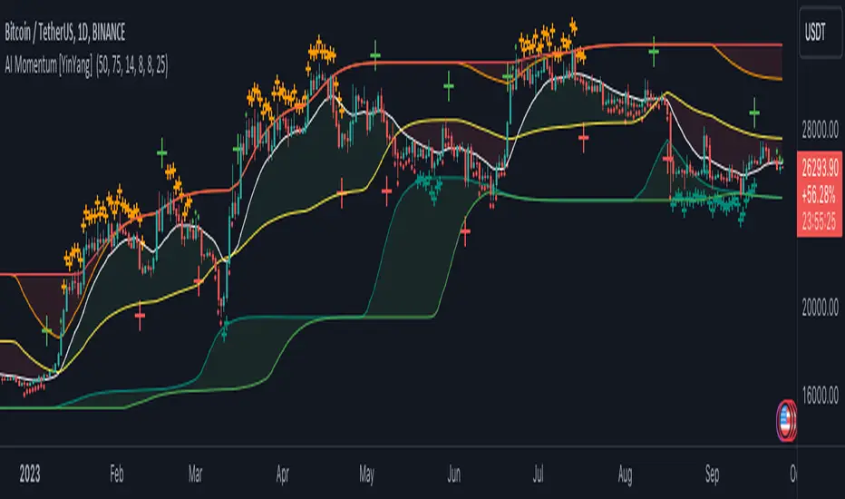
Machine Learning: Trend Pulse⚠️❗ Important Limitations: Due to the way this script is designed, it operates specifically under certain conditions:
Stocks & Forex : Only compatible with timeframes of 8 hours and above ⏰
Crypto : Only works with timeframes starting from 4 hours and higher ⏰
❗Please note that the script will not work on lower timeframes.❗
Feature Extraction : It begins by identifying a window of past price changes. Think of this as capturing the "mood" of the market over a certain period.
Distance Calculation : For each historical data point, it computes a distance to the current window. This distance measures how similar past and present market conditions are. The smaller the distance, the more similar they are.
Neighbor Selection : From these, it selects 'k' closest neighbors. The variable 'k' is a user-defined parameter indicating how many of the closest historical points to consider.
Price Estimation : It then takes the average price of these 'k' neighbors to generate a forecast for the next stock price.
Z-Score Scaling: Lastly, this forecast is normalized using the Z-score to make it more robust and comparable over time.
Inputs:
histCap (Historical Cap) : histCap limits the number of past bars the script will consider. Think of it as setting the "memory" of model—how far back in time it should look.
sampleSpeed (Sampling Rate) : sampleSpeed is like a time-saving shortcut, allowing the script to skip bars and only sample data points at certain intervals. This makes the process faster but could potentially miss some nuances in the data.
winSpan (Window Size) : This is the size of the "snapshot" of market data the script will look at each time. The window size sets how many bars the algorithm will include when it's measuring how "similar" the current market conditions are to past conditions.
All these variables help to simplify and streamline the k-NN model, making it workable within limitations. You could see them as tuning knobs, letting you balance between computational efficiency and predictive accuracy.
AI Channels (Clustering) [LuxAlgo]The AI Channels indicator is constructed based on rolling K-means clustering, a common machine learning method used for clustering analysis. These channels allow users to determine the direction of the underlying trends in the price.
We also included an option to display the indicator as a trailing stop from within the settings.
🔶 USAGE
Each channel extremity allows users to determine the current trend direction. Price breaking over the upper extremity suggesting an uptrend, and price breaking below the lower extremity suggesting a downtrend. Using a higher Window Size value will return longer-term indications.
The "Clusters" setting allows users to control how easy it is for the price to break an extremity, with higher values returning extremities further away from the price.
The "Denoise Channels" is enabled by default and allows to see less noisy extremities that are more coherent with the detected trend.
Users who wish to have more focus on a detected trend can display the indicator as a trailing stop.
🔹 Centroid Dispersion Areas
Each extremity is made of one area. The width of each area indicates how spread values within a cluster are around their centroids. A wider area would suggest that prices within a cluster are more spread out around their centroid, as such one could say that it is indicative of the volatility of a cluster.
Wider areas around a specific extremity can indicate a larger and more spread-out amount of prices within the associated cluster. In practice price entering an area has a higher chance to break an associated extremity.
🔶 DETAILS
The indicator performs K-means clustering over the most recent Window Size prices, finding a number of user-specified clusters. See here to find more information on cluster detection.
The channel extremities are returned as the centroid of the lowest, average, and highest price clusters.
K-means clustering can be computationally expensive and as such we allow users to determine the maximum number of iterations used to find the centroids as well as the number of most historical bars to perform the indicator calculation. Do note that increasing the calculation window of the indicator as well as the number of clusters will return slower results.
🔶 SETTINGS
Window Size: Amount of most recent prices to use for the calculation of the indicator.
Clusters": Amount of clusters detected for the calculation of the indicator.
Denoise Channels: When enabled, return less noisy channels extremities, disabling this setting will return the exact centroids at each time but will produce less regular extremities.
As Trailing Stop: Display the indicator as a trailing stop.
🔹 Optimization
This group of settings affects the runtime performance of the script.
Maximum Iteration Steps: Maximum number of iterations allowed for finding centroids. Excessively low values can return a better script load time but poor clustering.
Historical Bars Calculation: Calculation window of the script (in bars).
SimilarityMeasuresLibrary "SimilarityMeasures"
Similarity measures are statistical methods used to quantify the distance between different data sets
or strings. There are various types of similarity measures, including those that compare:
- data points (SSD, Euclidean, Manhattan, Minkowski, Chebyshev, Correlation, Cosine, Camberra, MAE, MSE, Lorentzian, Intersection, Penrose Shape, Meehl),
- strings (Edit(Levenshtein), Lee, Hamming, Jaro),
- probability distributions (Mahalanobis, Fidelity, Bhattacharyya, Hellinger),
- sets (Kumar Hassebrook, Jaccard, Sorensen, Chi Square).
---
These measures are used in various fields such as data analysis, machine learning, and pattern recognition. They
help to compare and analyze similarities and differences between different data sets or strings, which
can be useful for making predictions, classifications, and decisions.
---
References:
en.wikipedia.org
cran.r-project.org
numerics.mathdotnet.com
github.com
github.com
github.com
Encyclopedia of Distances, doi.org
ssd(p, q)
Sum of squared difference for N dimensions.
Parameters:
p (float ) : `array` Vector with first numeric distribution.
q (float ) : `array` Vector with second numeric distribution.
Returns: Measure of distance that calculates the squared euclidean distance.
euclidean(p, q)
Euclidean distance for N dimensions.
Parameters:
p (float ) : `array` Vector with first numeric distribution.
q (float ) : `array` Vector with second numeric distribution.
Returns: Measure of distance that calculates the straight-line (or Euclidean).
manhattan(p, q)
Manhattan distance for N dimensions.
Parameters:
p (float ) : `array` Vector with first numeric distribution.
q (float ) : `array` Vector with second numeric distribution.
Returns: Measure of absolute differences between both points.
minkowski(p, q, p_value)
Minkowsky Distance for N dimensions.
Parameters:
p (float ) : `array` Vector with first numeric distribution.
q (float ) : `array` Vector with second numeric distribution.
p_value (float) : `float` P value, default=1.0(1: manhatan, 2: euclidean), does not support chebychev.
Returns: Measure of similarity in the normed vector space.
chebyshev(p, q)
Chebyshev distance for N dimensions.
Parameters:
p (float ) : `array` Vector with first numeric distribution.
q (float ) : `array` Vector with second numeric distribution.
Returns: Measure of maximum absolute difference.
correlation(p, q)
Correlation distance for N dimensions.
Parameters:
p (float ) : `array` Vector with first numeric distribution.
q (float ) : `array` Vector with second numeric distribution.
Returns: Measure of maximum absolute difference.
cosine(p, q)
Cosine distance between provided vectors.
Parameters:
p (float ) : `array` 1D Vector.
q (float ) : `array` 1D Vector.
Returns: The Cosine distance between vectors `p` and `q`.
---
angiogenesis.dkfz.de
camberra(p, q)
Camberra distance for N dimensions.
Parameters:
p (float ) : `array` Vector with first numeric distribution.
q (float ) : `array` Vector with second numeric distribution.
Returns: Weighted measure of absolute differences between both points.
mae(p, q)
Mean absolute error is a normalized version of the sum of absolute difference (manhattan).
Parameters:
p (float ) : `array` Vector with first numeric distribution.
q (float ) : `array` Vector with second numeric distribution.
Returns: Mean absolute error of vectors `p` and `q`.
mse(p, q)
Mean squared error is a normalized version of the sum of squared difference.
Parameters:
p (float ) : `array` Vector with first numeric distribution.
q (float ) : `array` Vector with second numeric distribution.
Returns: Mean squared error of vectors `p` and `q`.
lorentzian(p, q)
Lorentzian distance between provided vectors.
Parameters:
p (float ) : `array` Vector with first numeric distribution.
q (float ) : `array` Vector with second numeric distribution.
Returns: Lorentzian distance of vectors `p` and `q`.
---
angiogenesis.dkfz.de
intersection(p, q)
Intersection distance between provided vectors.
Parameters:
p (float ) : `array` Vector with first numeric distribution.
q (float ) : `array` Vector with second numeric distribution.
Returns: Intersection distance of vectors `p` and `q`.
---
angiogenesis.dkfz.de
penrose(p, q)
Penrose Shape distance between provided vectors.
Parameters:
p (float ) : `array` Vector with first numeric distribution.
q (float ) : `array` Vector with second numeric distribution.
Returns: Penrose shape distance of vectors `p` and `q`.
---
angiogenesis.dkfz.de
meehl(p, q)
Meehl distance between provided vectors.
Parameters:
p (float ) : `array` Vector with first numeric distribution.
q (float ) : `array` Vector with second numeric distribution.
Returns: Meehl distance of vectors `p` and `q`.
---
angiogenesis.dkfz.de
edit(x, y)
Edit (aka Levenshtein) distance for indexed strings.
Parameters:
x (int ) : `array` Indexed array.
y (int ) : `array` Indexed array.
Returns: Number of deletions, insertions, or substitutions required to transform source string into target string.
---
generated description:
The Edit distance is a measure of similarity used to compare two strings. It is defined as the minimum number of
operations (insertions, deletions, or substitutions) required to transform one string into another. The operations
are performed on the characters of the strings, and the cost of each operation depends on the specific algorithm
used.
The Edit distance is widely used in various applications such as spell checking, text similarity, and machine
translation. It can also be used for other purposes like finding the closest match between two strings or
identifying the common prefixes or suffixes between them.
---
github.com
www.red-gate.com
planetcalc.com
lee(x, y, dsize)
Distance between two indexed strings of equal length.
Parameters:
x (int ) : `array` Indexed array.
y (int ) : `array` Indexed array.
dsize (int) : `int` Dictionary size.
Returns: Distance between two strings by accounting for dictionary size.
---
www.johndcook.com
hamming(x, y)
Distance between two indexed strings of equal length.
Parameters:
x (int ) : `array` Indexed array.
y (int ) : `array` Indexed array.
Returns: Length of different components on both sequences.
---
en.wikipedia.org
jaro(x, y)
Distance between two indexed strings.
Parameters:
x (int ) : `array` Indexed array.
y (int ) : `array` Indexed array.
Returns: Measure of two strings' similarity: the higher the value, the more similar the strings are.
The score is normalized such that `0` equates to no similarities and `1` is an exact match.
---
rosettacode.org
mahalanobis(p, q, VI)
Mahalanobis distance between two vectors with population inverse covariance matrix.
Parameters:
p (float ) : `array` 1D Vector.
q (float ) : `array` 1D Vector.
VI (matrix) : `matrix` Inverse of the covariance matrix.
Returns: The mahalanobis distance between vectors `p` and `q`.
---
people.revoledu.com
stat.ethz.ch
docs.scipy.org
fidelity(p, q)
Fidelity distance between provided vectors.
Parameters:
p (float ) : `array` 1D Vector.
q (float ) : `array` 1D Vector.
Returns: The Bhattacharyya Coefficient between vectors `p` and `q`.
---
en.wikipedia.org
bhattacharyya(p, q)
Bhattacharyya distance between provided vectors.
Parameters:
p (float ) : `array` 1D Vector.
q (float ) : `array` 1D Vector.
Returns: The Bhattacharyya distance between vectors `p` and `q`.
---
en.wikipedia.org
hellinger(p, q)
Hellinger distance between provided vectors.
Parameters:
p (float ) : `array` 1D Vector.
q (float ) : `array` 1D Vector.
Returns: The hellinger distance between vectors `p` and `q`.
---
en.wikipedia.org
jamesmccaffrey.wordpress.com
kumar_hassebrook(p, q)
Kumar Hassebrook distance between provided vectors.
Parameters:
p (float ) : `array` 1D Vector.
q (float ) : `array` 1D Vector.
Returns: The Kumar Hassebrook distance between vectors `p` and `q`.
---
github.com
jaccard(p, q)
Jaccard distance between provided vectors.
Parameters:
p (float ) : `array` 1D Vector.
q (float ) : `array` 1D Vector.
Returns: The Jaccard distance between vectors `p` and `q`.
---
github.com
sorensen(p, q)
Sorensen distance between provided vectors.
Parameters:
p (float ) : `array` 1D Vector.
q (float ) : `array` 1D Vector.
Returns: The Sorensen distance between vectors `p` and `q`.
---
people.revoledu.com
chi_square(p, q, eps)
Chi Square distance between provided vectors.
Parameters:
p (float ) : `array` 1D Vector.
q (float ) : `array` 1D Vector.
eps (float)
Returns: The Chi Square distance between vectors `p` and `q`.
---
uw.pressbooks.pub
stats.stackexchange.com
www.itl.nist.gov
kulczynsky(p, q, eps)
Kulczynsky distance between provided vectors.
Parameters:
p (float ) : `array` 1D Vector.
q (float ) : `array` 1D Vector.
eps (float)
Returns: The Kulczynsky distance between vectors `p` and `q`.
---
github.com

Hybrid EMA AlgoLearner⭕️Innovative trading indicator that utilizes a k-NN-inspired algorithmic approach alongside traditional Exponential Moving Averages (EMAs) for more nuanced analysis. While the algorithm doesn't actually employ machine learning techniques, it mimics the logic of the k-Nearest Neighbors (k-NN) methodology. The script takes into account the closest 'k' distances between a short-term and long-term EMA to create a weighted short-term EMA. This combination of rule-based logic and EMA technicals offers traders a more sophisticated tool for market analysis.
⭕️Foundational EMAs: The script kicks off by generating a 50-period short-term EMA and a 200-period long-term EMA. These EMAs serve a dual purpose: they provide the basic trend-following capability familiar to most traders, akin to the classic EMA 50 and EMA 200, and set the stage for more intricate calculations to follow.
⭕️k-NN Integration: The indicator distinguishes itself by introducing k-NN (k-Nearest Neighbors) logic into the mix. This machine learning technique scans prior market data to find the closest 'neighbors' or distances between the two EMAs. The 'k' closest distances are then picked for further analysis, thus imbuing the indicator with an added layer of data-driven context.
⭕️Algorithmic Weighting: After the k closest distances are identified, they are utilized to compute a weighted EMA. Each of the k closest short-term EMA values is weighted by its associated distance. These weighted values are summed up and normalized by the sum of all chosen distances. The result is a weighted short-term EMA that packs more nuanced information than a simple EMA would.
Machine Learning Regression Trend [LuxAlgo]The Machine Learning Regression Trend tool uses random sample consensus (RANSAC) to fit and extrapolate a linear model by discarding potential outliers, resulting in a more robust fit.
🔶 USAGE
The proposed tool can be used like a regular linear regression, providing support/resistance as well as forecasting an estimated underlying trend.
Using RANSAC allows filtering out outliers from the input data of our final fit, by outliers we are referring to values deviating from the underlying trend whose influence on a fitted model is undesired. For financial prices and under the assumptions of segmented linear trends, these outliers can be caused by volatile moves and/or periodic variations within an underlying trend.
Adjusting the "Allowed Error" numerical setting will determine how sensitive the model is to outliers, with higher values returning a more sensitive model. The blue margin displayed shows the allowed error area.
The number of outliers in the calculation window (represented by red dots) can also be indicative of the amount of noise added to an underlying linear trend in the price, with more outliers suggesting more noise.
Compared to a regular linear regression which does not discriminate against any point in the calculation window, we see that the model using RANSAC is more conservative, giving more importance to detecting a higher number of inliners.
🔶 DETAILS
RANSAC is a general approach to fitting more robust models in the presence of outliers in a dataset and as such does not limit itself to a linear regression model.
This iterative approach can be summarized as follow for the case of our script:
Step 1: Obtain a subset of our dataset by randomly selecting 2 unique samples
Step 2: Fit a linear regression to our subset
Step 3: Get the error between the value within our dataset and the fitted model at time t , if the absolute error is lower than our tolerance threshold then that value is an inlier
Step 4: If the amount of detected inliers is greater than a user-set amount save the model
Repeat steps 1 to 4 until the set number of iterations is reached and use the model that maximizes the number of inliers
🔶 SETTINGS
Length: Calculation window of the linear regression.
Width: Linear regression channel width.
Source: Input data for the linear regression calculation.
🔹 RANSAC
Minimum Inliers: Minimum number of inliers required to return an appropriate model.
Allowed Error: Determine the tolerance threshold used to detect potential inliers. "Auto" will automatically determine the tolerance threshold and will allow the user to multiply it through the numerical input setting at the side. "Fixed" will use the user-set value as the tolerance threshold.
Maximum Iterations Steps: Maximum number of allowed iterations.
